Article

Research on Projection Filtering Method Based on Projection Symmetric Interval and Its Application in Underwater Navigation

1
Hubei Key Laboratory of Digital Textile Equipment, Wuhan Textile University, Wuhan 430200, China
2
School of Mechanical Engineering & Automation, Wuhan Textile University, Wuhan 430200, China
*
Author to whom correspondence should be addressed.
Symmetry 2021, 13(9), 1715; https://doi.org/10.3390/sym13091715
Submission received: 29 June 2021 / Revised: 7 September 2021 / Accepted: 8 September 2021 / Published: 16 September 2021

Abstract

:
For non-linear systems (NLSs), the state estimation problem is an essential and important problem. This paper deals with the nonlinear state estimation problems in nonlinear and non-Gaussian systems. Recently, the Bayesian filter designer based on the Bayesian principle has been widely applied to the state estimation problem in NLSs. However, we assume that the state estimation models are nonlinear and non-Gaussian, applying traditional, typical nonlinear filtering methods, and there is no precise result for the system state estimation problem. Therefore, the larger the estimation error, the lower the estimation accuracy. To perfect the imperfections, a projection filtering method (PFM) based on the Bayesian estimation approach is applied to estimate the state. First, this paper constructs its projection symmetric interval to select the basis function. Second, the prior probability density of NLSs can be projected into the basis function space, and the prior probability density solution can be solved by using the Fokker–Planck Equation (FPE). According to the Bayes formula, the proposed estimator utilizes the basis function in projected space to iteratively calculate the posterior probability density; thus, it avoids calculating the partial differential equation. By taking two illustrative examples, it is also compared with the traditional UKF and PF algorithm, and the numerical experiment results show the feasibility and effectiveness of the novel nonlinear state estimation filter algorithm.

1. Introduction

In recent years, the state estimation problems of the dynamic system have become very important in various applications of nonlinear systems (NLSs), such as underwater navigation positioning, mechanical equipment fault diagnosis, signal processing, space target orbit prediction, target tracking, etc. [1,2,3].
The earliest applied state estimation method is the Kalman filter method. The Kalman Filter (KF) in [4] is a state filter estimator based on the minimum mean square error (MMSE). The KF method is only suitable for the state estimation model in linear and Gaussian systems. However, the state estimation problems of many actual physical systems are nonlinear and non-Gaussian models. If KF is used to solve the state estimation problem in NLSs, the estimation error will be divergent, the estimation accuracy will be low, and the estimation result will not be convergent. In order to overcome these problems, many scholars have studied many sub-optimal estimators and evaluated the Extended Kalman Filter (EKF) in navigation in the literature [5]. The basic principle is to linearize the nonlinear system and use KF to solve the linear system. The final result is that when the linearization error becomes larger, the estimation accuracy is low. EKF is only effective for nonlinear systems that are approximately linear in the update interval, so it is difficult to apply to many physical systems. Subsequently, the Unscented Kalman Filter (UKF) in the literature [6] shows that the UKF method assumes that the system noise conforms to the Gaussian distribution and does not require the system to be approximately linear. For nonlinear systems, the performance of the UKF method is better than that of EKF. Although UKF has achieved good results in many navigation application systems [7,8,9], the UKF method should satisfy three conditions: (1) State estimation models of the nonlinear systems should be given in detail. (2) The deviation of the reference state trajectory must small. (3) The conditional Probability Density Function (PDF) should satisfy the Gaussian distribution. Otherwise, the performance of UKF will become unstable. Therefore, this is not suitable for general methods of state estimation problems.
There is another popular Bayesian estimation algorithm based on the Particle Filter method (PF) in NLSs [10], also known as a complex technique based on the sequential Monte Carlo (SMC) method, which was initiated by Gordon and Salmond et al. in 1993 [11]. This method is a non-parametric sequential Monte-Carlo analog recursive filtering algorithm based on the Bayesian estimate principle. The basic principle of PF is that it can approximate the posterior probability density of the state estimation system by applying a random sampled particle with different weights; according to the Bayesian principle, it can update the posterior probability density by introducing observation values. In the past two decades, many scholars have conducted a lot of studies to improve the performance of PF. They have successively proposed that auxiliary particle filters in [12], unscented particle filters in [13] and Gaussian particle filters in [14] can effectively improve particle importance resampling and particle degeneracy phenomena. In [15], particle filtering could effectively improve estimation accuracy and computational efficiency. PF can deal with a set of nonlinear, non-Gaussian state estimation problems. However, it still has some shortcomings, such as computational complexity and sample degradation.
In the past ten years, many scholars have widely proposed Bayesian estimators in the state estimation problems of a dynamic system [16,17,18,19]. An adaptive Kalman filter estimator in [20] was proposed to solve state estimation problems. Theoretically speaking, a state estimation model in NLSs can be denoted by Fokker–Planck Equations (FPEs) and the Bayesian estimation equation. While the former is a partial differential equation and can show how to use the PDF of the nonlinear system to update the state, the latter can use new measure data to update the measurement information [21].
In [22], a projection filter method has been proposed, which can only solve the problem of low-dimensional state estimation. To fill this gap, the Projection Filter Method (PFM) is given in this paper and is a classic method for solving the Fokker–Planck equation (FPE). PFM assumes that the numerical solution of FPE can be represented by a set of basis functions in a projection space. Inspired by [23,24], an accurate probability solution is obtained by a set of orthogonal basis functions. In fact, compared with PF or other classic filter methods (such as UKF and EKF), PFM has more advantages than others, such as computational speed and convergence.
This paper is organized as follows. In Section 2, a state estimation model in NLSs is given, and the probability solution of the state estimation problem is defined. In Section 3, the PFM program is divided into two parts to solve the state estimation problems: status update and measurement update. Section 3 also introduces how to select the basis function based on the projected symmetric interval. Then, illustrative examples and their simulation results are given in Section 4. In Section 5, the conclusions of this paper are analyzed in detail.

2. Background and Problem Formulation

2.1. State Estimation Model in NLSs

Actually, in most non-linear systems (NLSs), given the distribution of initial state x 0 , the state equations of most physical systems will develop with continuous time t , and the measurement equations can only be performed periodically at discrete time t k . Assume that the n-dimensional state estimation model can be denoted as
d x t = f x t , t d t + g d β t
z k = h x k , t k + v k
where x t n denotes the n-dimensional system state vector, f x t , t : n × n denotes the state transfer matrix, z k m is the measurement vector, h x k , t k : n × m is the measurement matrix and g : n × n × d denotes the diffusion coefficient matrix. β t denotes a d-dimensional standard Brownian motion vector, and v k denotes a m-dimensional measured noise vector. Based on this, we have the following:
Ε β t = 0 , Ε β t β t T = Q t E v k = 0 , E v k v k T = R k E v k β t T = 0
where R k and Q t denote the covariance matrices of the Brownian motion process and measured noise vector.

2.2. Probability Solution of State Estimation Problem

According to the Bayesian filter estimation principle [17], the state estimation model needs to estimate the system state. Suppose that the posterior probability density distribution p x , t k + 1 | z k + 1 of some dynamics system satisfies
p x , t k + 1 | z k + 1 = p z k + 1 | x p x , t k + 1 | z k Ω p z k + 1 | x p x , t k + 1 | z k d x
where the likelihood probability density p z k + 1 | x is defined as
p z k + 1 | x = 1 2 π m R k + 1 e x p 1 2 z k + 1 h x k , t k + 1 T R k + 1 1 z k + 1 h x k , t k + 1
where h x k , t k + 1 denotes the measurement matrix in (2) and represents the measurement vector in state space, and R k is expressed as the covariance matrix in Equation (3). p x , t k + 1 | z k is prior probability density, and the prior probability density of the nonlinear system will satisfy the Fokker–Planck Equation (FPE) [21]:
L p = p ˙ = 1 2 r , s = 1 n 2 g Q t g T p x r x s r = 1 n f x t , t p x r
where probability density function (PDF) p = p x , t | z t is expressed as the probability solution of FPE. Assume that the initial probability distribution is p x 0 , t 0 | z 0 = p 0 .

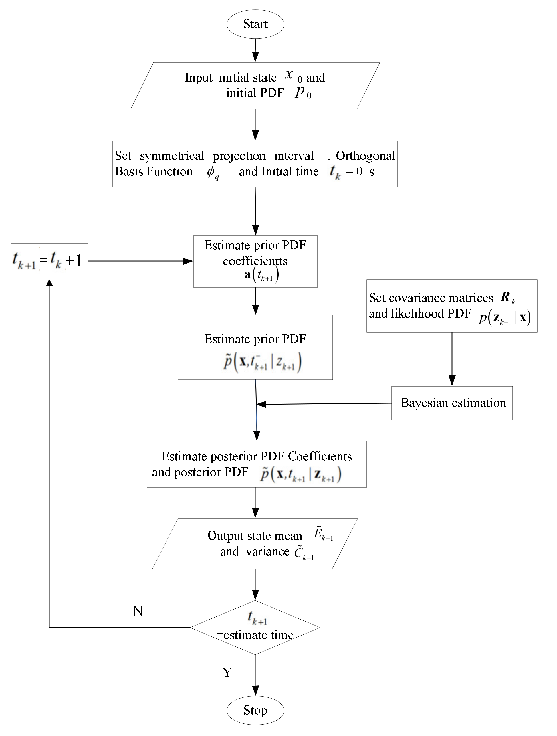
3. Nonlinear Filter Estimator Design-Based Projection Filter Method

The Projection Filter Method (PFM) is a state estimation method that approximates the PDF of the state based on projection symmetric interval and basis function. To construct a set of finite-dimensional orthogonal basis functions in the projection space, the state can be projected into the basis function space, and the PFM uses the FPE to obtain the PDF of the state in the projection space. The problem of solving Partial Differential Equations (PDEs) (such as FPE) is transformed into a problem of solving linear ordinary differential equations. In this part, the numerical solution is simplified to avoid calculating PDEs. PFM is a useful numerical calculation method for solving a state estimation problem. The flowchart of a filter estimator design (PFM) is shown in Figure 1.
Research manuscripts reporting large datasets that are deposited in a publicly available database should specify where the data have been deposited and provide the relevant accession numbers. If the accession numbers have not yet been obtained at the time of submission, please state that they will be provided during the review. They must be provided prior to publication.
Interventionary studies involving animals or humans, and other studies that require ethical approval, must list the authority that provided approval and the corresponding ethical approval code.

3.1. Status Update

Suppose n-dimension state vector x = x 1 , , x n , the PDF in NLSs can be denoted as p x , t . For a fixed time t 0 , assume that the PDF in NLSs can be expressed by an infinite sum of basis functions in the projection space
p x , t = i = 0 m i t ϕ i x
where ϕ i x denotes the orthogonal basis function in the projection subspace, m i t = p x , t , ϕ i x denotes the coefficients of p x , t in (1), and, ϕ denotes the inner product, so η , ϕ = Ω η x ϕ x d x , Ω R n .
Equality L 2 is in the sense of the norm, and V N = s p a n ϕ i 0 N 1 V denotes a complete set of basis functions for L 2 . p x , t could be expressed as the following form:
p ˜ x , t = i = 0 N 1 m i t ϕ i x
where unknown coefficients m i t satisfy m i t = p x , t , ϕ i x . These basis functions ϕ i x should satisfy the following orthogonality properties:
M q + 1 , i + 1 = ϕ i , ϕ q = 0 i q 1 i = q
where i , q = 0 , 1 , 2 , , N 1 .
So, M can be given as M = E N × N .
Assume that a t = m 0 t m 1 t m N 1 t T and Φ x = ϕ 0 x ϕ 1 x ϕ N 1 x T .
p x , t in (7) will be denoted as p x , t = m t T Φ x .
In function space L 2 R n , basic functions such as ϕ i x are known. To solve the coefficients matrix m t , the approximate PDF solution can be solved.
Having substituted Formula (8) into Formula (6), we can obtain
i = 0 N 1 m i ϕ i t = i = 0 N 1 m i 1 2 r , s = 1 n 2 g Q t g T ϕ i x r x s i = 0 N 1 m i r = 1 n f x , t ϕ i x r
Having projected Equation (10) onto the space V N = s p a n ϕ q 0 N 1 , we can obtain
i = 0 N 1 m i ϕ i , ϕ q t = i = 0 N 1 m i 1 2 r , s = 1 n 2 g Q t g T ϕ i x r x s , ϕ q i = 0 N 1 m i r = 1 n f x , t ϕ i x r , ϕ q
If Q , f and g are independent of time t , Equation (10) can be rewritten as
i = 0 N 1 m ˙ i ϕ i , ϕ q = i = 0 N 1 m i 1 2 r , s = 1 n 2 g Q t g T ϕ i x r x s , ϕ q i = 0 N 1 m i r = 1 n f x , t ϕ i x r , ϕ q
Equation (12) denotes a linear ordinary differential equation that may be written in matrix notation by defining
g Q g T = B
M q , i = ϕ i - 1 , ϕ q - 1 = 1 i = q 0 i q
We have
A q + 1 , i + 1 = 1 2 r , s = 1 n B 2 ϕ i x r x s r = 1 n f x , t ϕ i x r , ϕ q  
where i , q = 0 , 1 , N 1 , A q i is the element of matrix A in Equation (15).
With these definitions M = E N × N , and Equation (12) can be rewritten as
M m ˙ t = A m t
Due to M = E N × N , Equation (16) can be rewritten as
m ˙ t = A m t
According to initial density function p 0 = p x 0 , t 0 | z 0 , at time t = t 0 , the initial coefficients a t 0 can be obtained as
p 0 , ϕ j = i = 0 N 1 m i t 0 ϕ i , ϕ j = i = 0 N 1 m i t 0 ϕ i , ϕ j
s = p 0 , ϕ 0 p 0 , ϕ N 1 T
m t 0 = M 1 s = s
Having substituted Equation (20) into Equation (17), we have
m t = e x p t 0 t A d τ s
If it is independent of time in t k , t k + 1 , Equation (11) has the following simple solution:
m t = e x p A t t k m t k , t t k , t k + 1
A priori coefficients can be obtained:
m t k + 1 = e x p A t k + 1 t k m t k
where a t k are the posterior coefficients at time t k .
A priori probability density is given as
p ˜ x , t k + 1 | z k + 1 = i = 0 N 1 m i t k + 1 ϕ i = m t k + 1 T Φ x

3.2. Measurement Update

Due to the Bayesian formula (Equation (6), the posterior PDF can be expressed as
p x , t k + 1 | z k + 1 = i = 0 m i t k + 1 ϕ i
We approximate p x , t k + 1 | z k + 1 by truncating the sum
p ˜ x , t k + 1 | z k + 1 = i = 0 N 1 m i t k + 1 ϕ i
Notice that the parameters m i t k + 1 are unknown. The accurate propagation of the PDF requires the solution of new parameters m i t k + 1 .
Having projected the posterior PDF in Equation (26) onto the projection space V N = s p a n ϕ q 0 N 1 , we can obtain
p ˜ x , t k + 1 | z k + 1 , ϕ q = i = 0 N 1 m i t k + 1 ϕ i , ϕ q = p z k + 1 | x i = 0 N 1 m i t k + 1 ϕ i , ϕ q Ω p z k + 1 | x i = 0 N 1 m i t k + 1 ϕ i d x = i = 0 N 1 m i t k + 1 p z k + 1 | x ϕ i , ϕ q i = 0 N 1 m i t k + 1 p z k + 1 | x , ϕ i
where q = 0 , 1 , N 1 .
The parameters of the posterior probability density are given by
m t k + 1 = F k + 1 m t k + 1 K k + 1 T m t k + 1
where
F k + 1 q i = p z k + 1 | x ϕ i , ϕ q K k + 1 i = p z k + 1 | x , ϕ i
By substituting Equation (29) into Equation (28), the posterior PDF is given by
p ˜ x , t k + 1 | z k + 1 = i = 0 N 1 m i t k + 1 ϕ i
According to the posterior PDF p ˜ x , t k + 1 | z k + 1 in Equation (30), the conditional mean E ˜ x , t k + 1 | z k + 1 = E ˜ k + 1 and the variance C ˜ x , t k + 1 | z k + 1 = C ˜ k + 1 are given by the following equations:
E ˜ x , t k + 1 | z k + 1 = Ω η p ˜ η , t k + 1 | z k + 1 d η i = 0 N 1 m i t k + 1 Ω ϕ i η d η
C ˜ x , t k + 1 | z k + 1 = Ω η E ˜ x , t k + 1 | z k + 1 2 p ˜ η , t k + 1 | z k + 1 d η i = 0 N 1 m i t k + 1 Ω ϕ i η E ˜ x , t k + 1 | z k + 1 2 d η

3.3. Selecting Basis Function Based on Projection Symmetric Interval

Steps of PFM-PSI (Projection Filter Method based on Projection Symmetric Interval) in the n-dimensional system can be obtained as:
(1) In n -dimensional state space, according to Ε ˜ k + 1 and C ˜ k + 1 in Equation (32), a symmetric interval b , c is given by
b = x x = E k 10 C k c = x x = E k + 10 C k
Assume that the coordinate series x i are given by
x i = i c i b i K + b i , i = 0 , 1 , , K
where K is the interval number and is given by a positive integer.
Assume that the orthogonal complex exponential basis functions in [25,26] are given by
ϕ q x = 1 c q b q e x p j 2 π q x b q c q b q ϕ q x = 1 c q b q e x p j 2 π q x b q c q b q
where q = 0 , 1 , N 1 .
We have M = E N × N , and projection space can be expressed as V N = s p a n ϕ q 0 N 1 V . The posterior coefficients m t k at time t k are given by
m t k = a 0 t k a 1 t k a N 1 t k Τ
The optimum value of the number N of basis functions can be obtained by the initial state.
(2) Calculate prior coefficients m t k + 1 at time t k + 1 .
By calculating the posterior probability density p x , t k at time t k , the prior coefficients m t k + 1 at time t k + 1 can be obtained as
p x , t k , ϕ q i = 0 N 1 a i t k ϕ i , ϕ q
m t k = s
Due to the property of the probability density Ω p ˜ x d x = 1 , we have
b c p ˜ x d x = b c r e a l i = 0 N 1 a i ϕ i d x = i = 0 N 1 r e a l b c a i ϕ i d x = c b I F F T 1 r e a l m = 1
We can obtain
m t k = m t k / c b I F F T 1 r e a l m t k
Projecting FPE onto the subspace V N , we have
A q i = 1 2 2 g Q g T ϕ i x 2 f ϕ i x , ϕ q = c b K 2 F F T 1 2 2 g Q g T ϕ i x 2 f ϕ i x q
where g and K are the constant matrix, we have
A q i = c b K F F T 1 2 g Q g T 2 ϕ i x 2 f ϕ i x x = x n q = c b K F F T 1 2 g Q g T 2 π i c b 2 ϕ i f x ϕ i + f j 2 π i c b ϕ i x = x n q
the prior coefficients in Equation (23) can be obtained as
m t k + 1 = exp A t k + 1 t k m t k
By exploiting prior coefficients, normalization processing is carried out as
m t k + 1 = m t k + 1 / c b i = 0 K 1 I F F T 1 r e a l m t k + 1
(3) Calculate posterior coefficients m t k + 1 .
F k + 1 q i = p z k + 1 | x ϕ i , ϕ q = c b K F F T 1 p z k + 1 | x ϕ i x = x n q
E k + 1 i = p z k + 1 | x , ϕ i * = c b K I F F T 1 p z k + 1 | x x = x n i
where i , q = 0 , 1 , N 1 . In matrix notation,
m t k + 1 = F k + 1 m t k + 1 E k + 1 T m t k + 1
Due to coefficients m t k + 1 in Equation (47), normalization processing is carried out as
m t k + 1 = m t k + 1 / c b i = 0 K 1 I F F T 1 r e a l m t k + 1
(4) Calculating conditional mean E ˜ k + 1 and variance C ˜ k + 1 , posterior probability density function can be formulated as
p ˜ x , t k + 1 | z k + 1 = i = 0 N 1 m i t k + 1 ϕ i
According to the posterior PDF, the state estimate mean E ˜ k + 1 can be evaluated as
E ˜ k + 1 = b c η p ˜ η , t k + 1 | z k + 1 d η = b c η r e a l i = 0 N 1 a i t k + 1 ϕ i d η = r e a l i = 0 N 1 m i t k + 1 b c η ϕ i d η = r e a l Ψ T m t k + 1
where Ψ = c b K I F F T 1 x n .
The state estimate variance C ˜ k + 1 can be given as
C ˜ k + 1 = b c η x ^ 2 p ˜ η , t k + 1 | z k + 1 d η = r e a l i = 0 N 1 m i t k + 1 b c η E ^ x | z k + 1 2 ϕ i d η = r e a l Γ T m t k + 1
where Γ = c b K I F F T 1 x n x ^ x n x ^ .
(5) Approximation of mean and variance are used to calculate a priori coefficients at time t k + 2 .

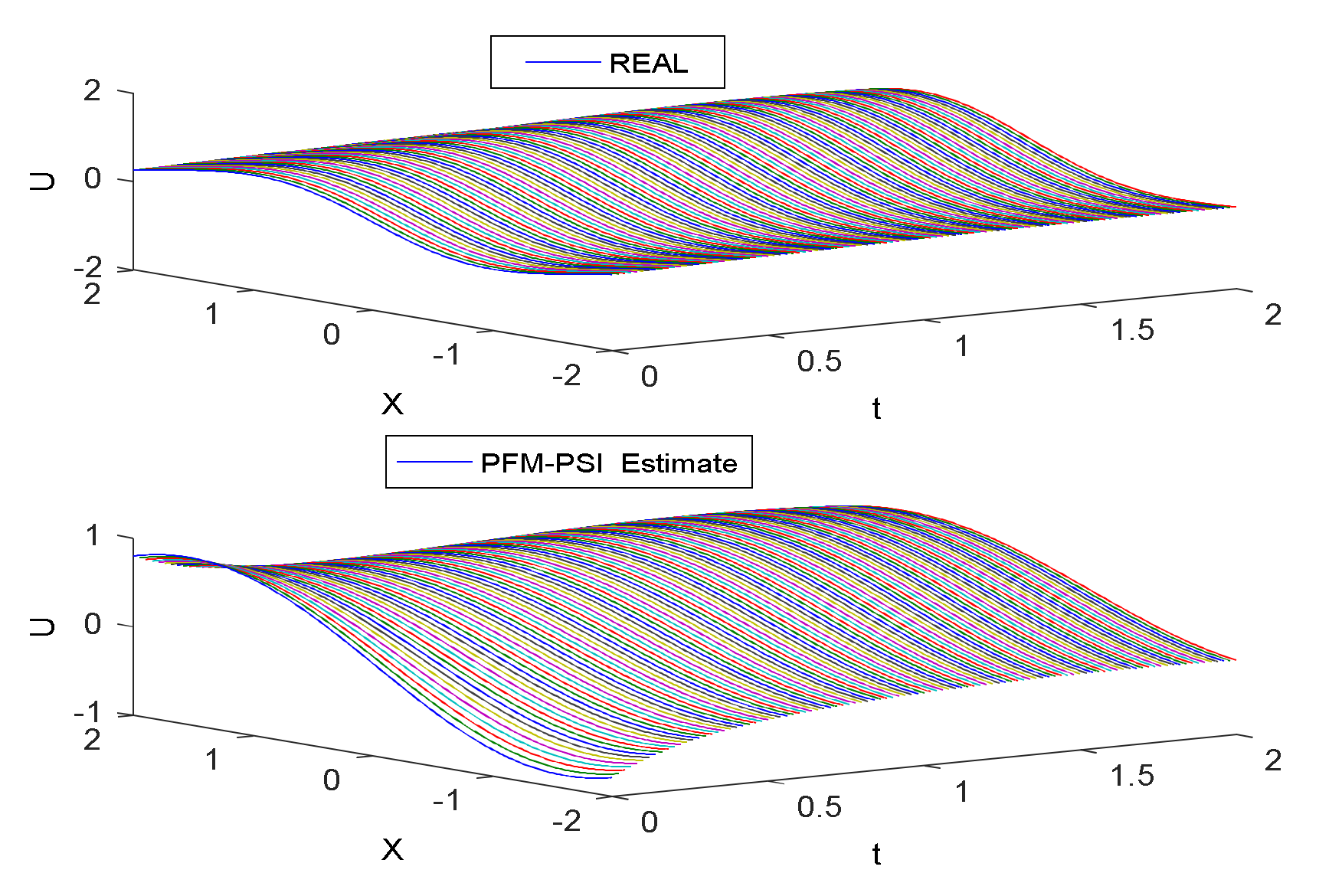
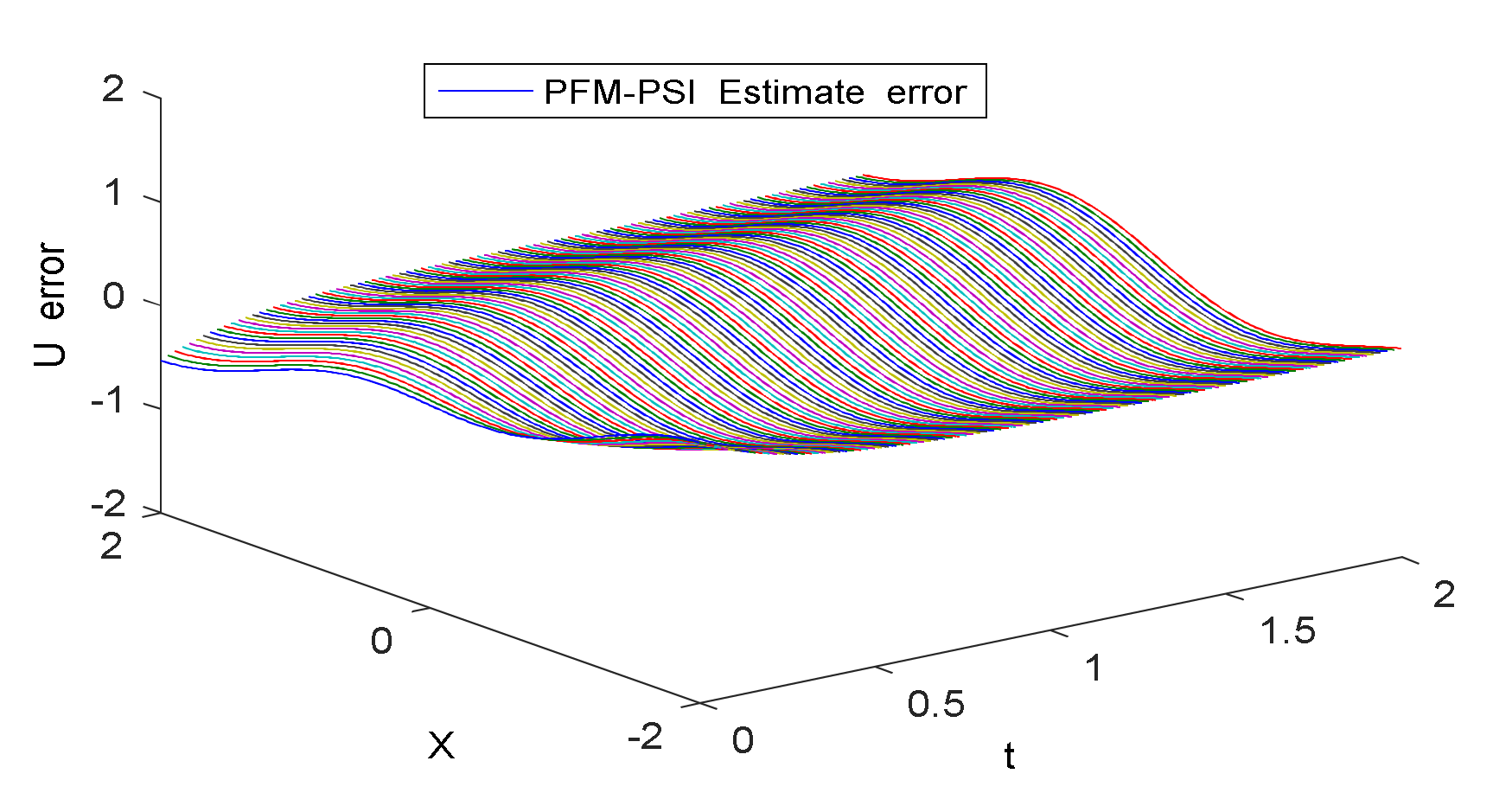
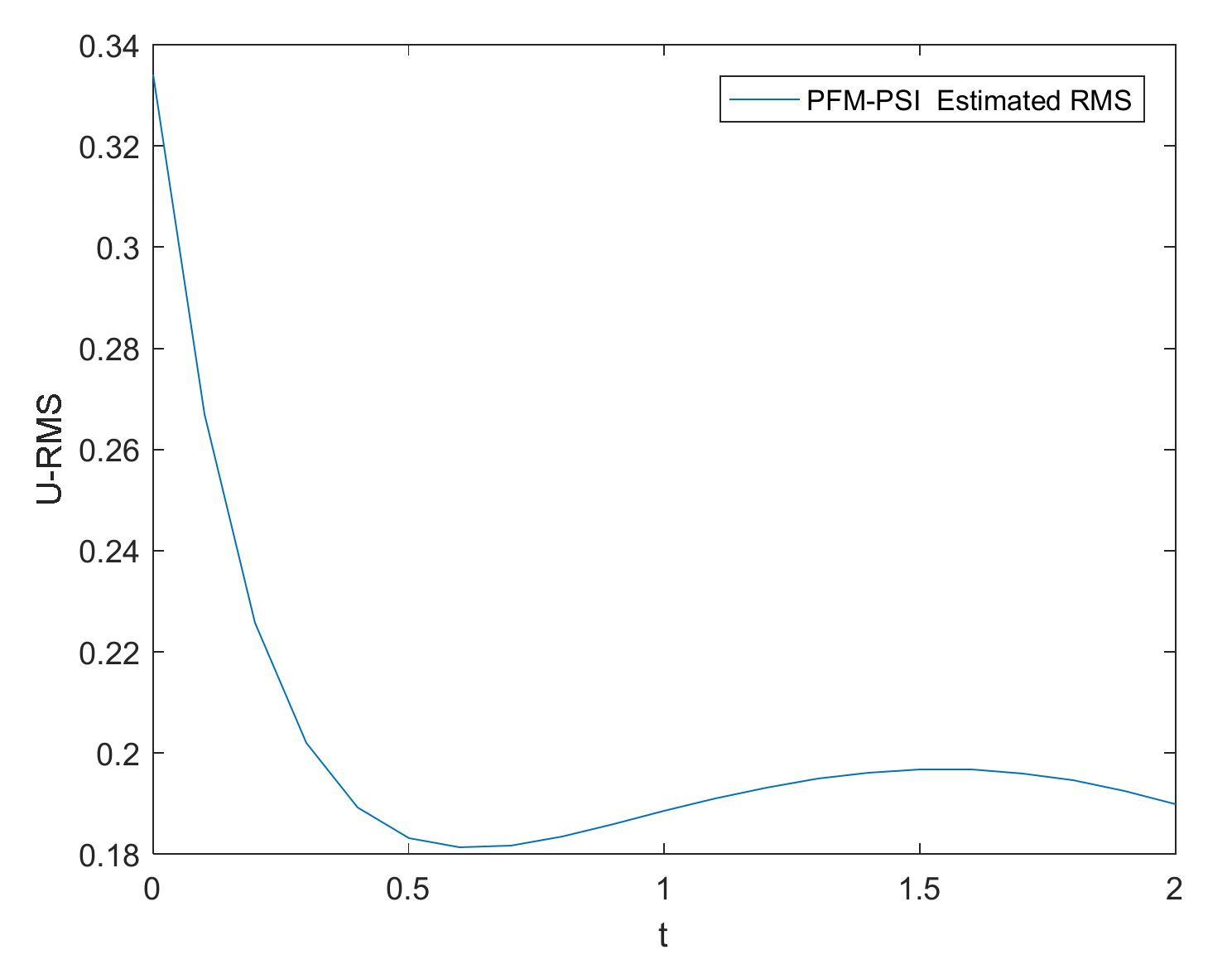
4. Illustrative Examples and Simulations

4.1. Example 1

For the first example, the state estimation model will be given by the following dynamic system with the real solution in [27,28]:
u t = u x x x 2 u + s i n t + c o s t + 3 x e x 2 2
u x , t = s i n t + x e x 2 2
It is easy to obtain that u x , t = sin t + x e x 2 2 is the exact solution of Equation (52). The initial state is u 0 , 0 = 0 .
Here, using PFM-PSI (Projection Filter Method based on Projection Symmetric Interval), the interval of time is chosen as 1 s. The performance output of PFM-PSI is shown in Figure 2, Figure 3 and Figure 4. The posterior PDFs are plotted. The normalized density functions are plotted every other 0.1 s. The results of both real solution and PFM–PSI have been plotted in Figure 2. Having compared the estimated PDF and the true PDF of the state in Figure 3, we give the estimated error and root mean square (RMS) of PFM in Figure 3 and Figure 4. Obviously, for a nonlinear system, PFM–PSI has the effectiveness of the new state estimator algorithm.

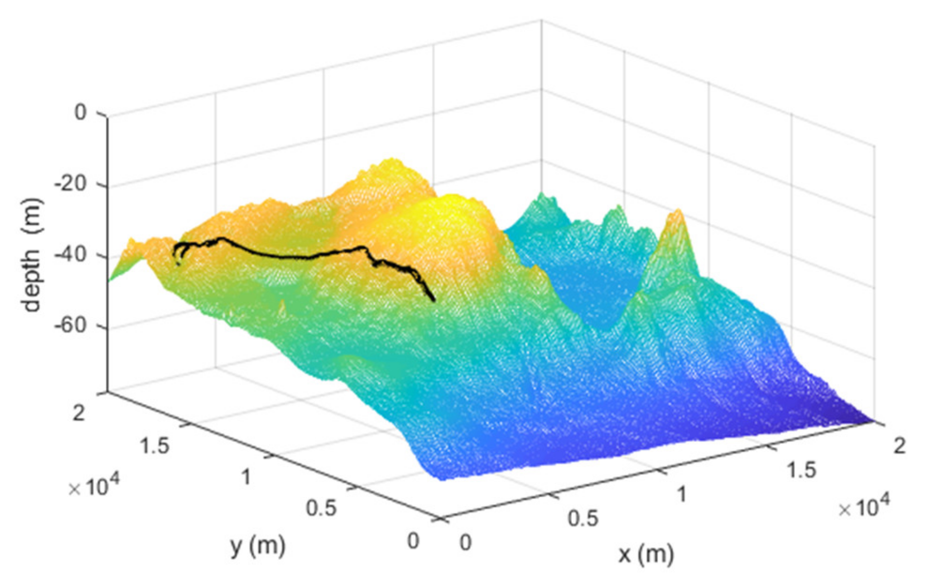
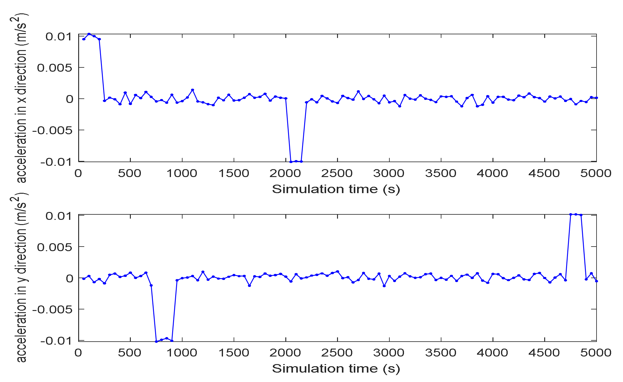
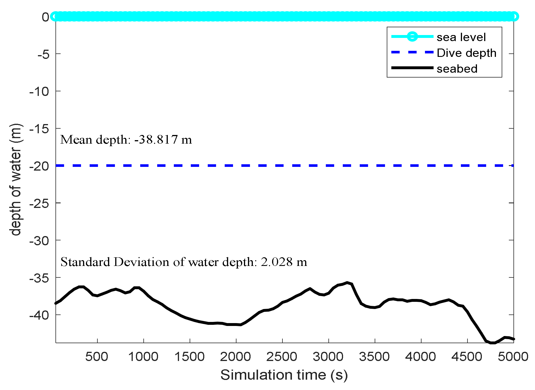
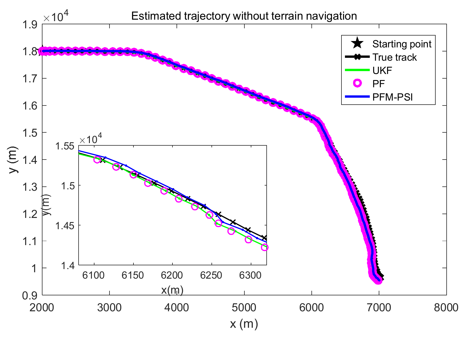
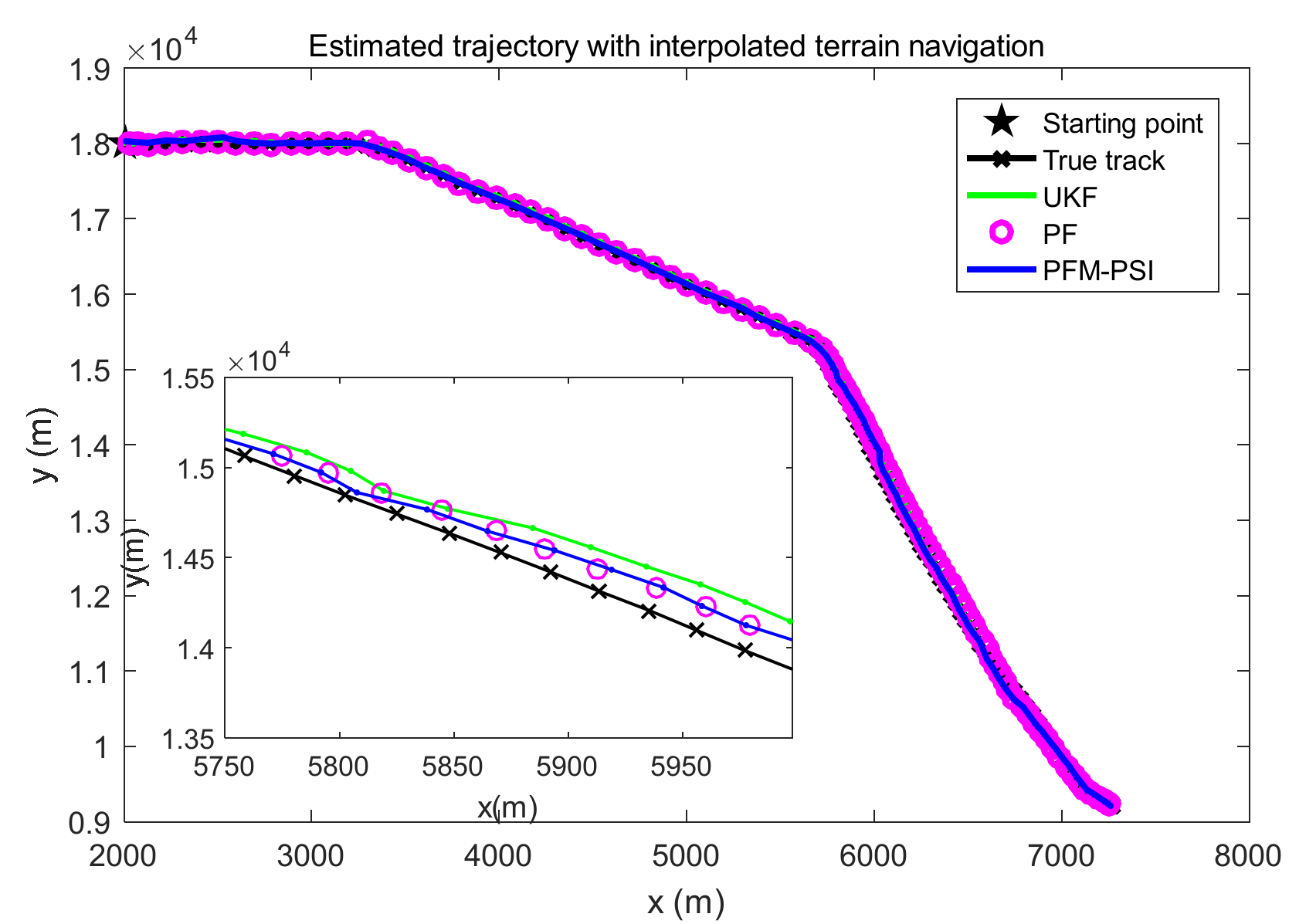
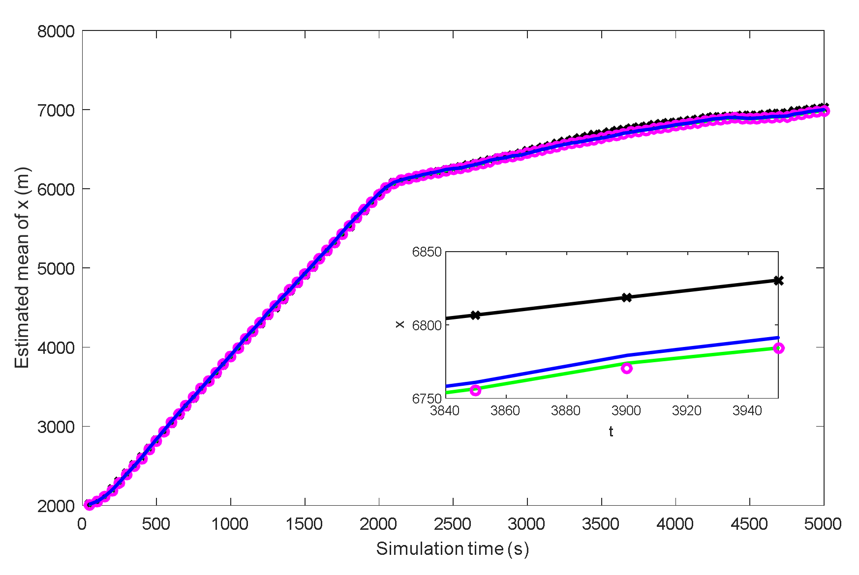
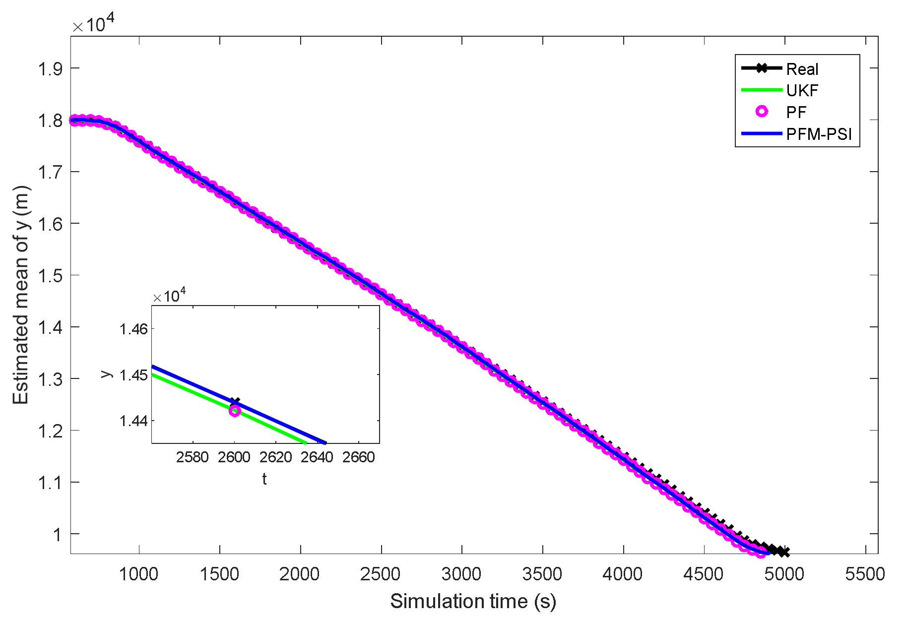
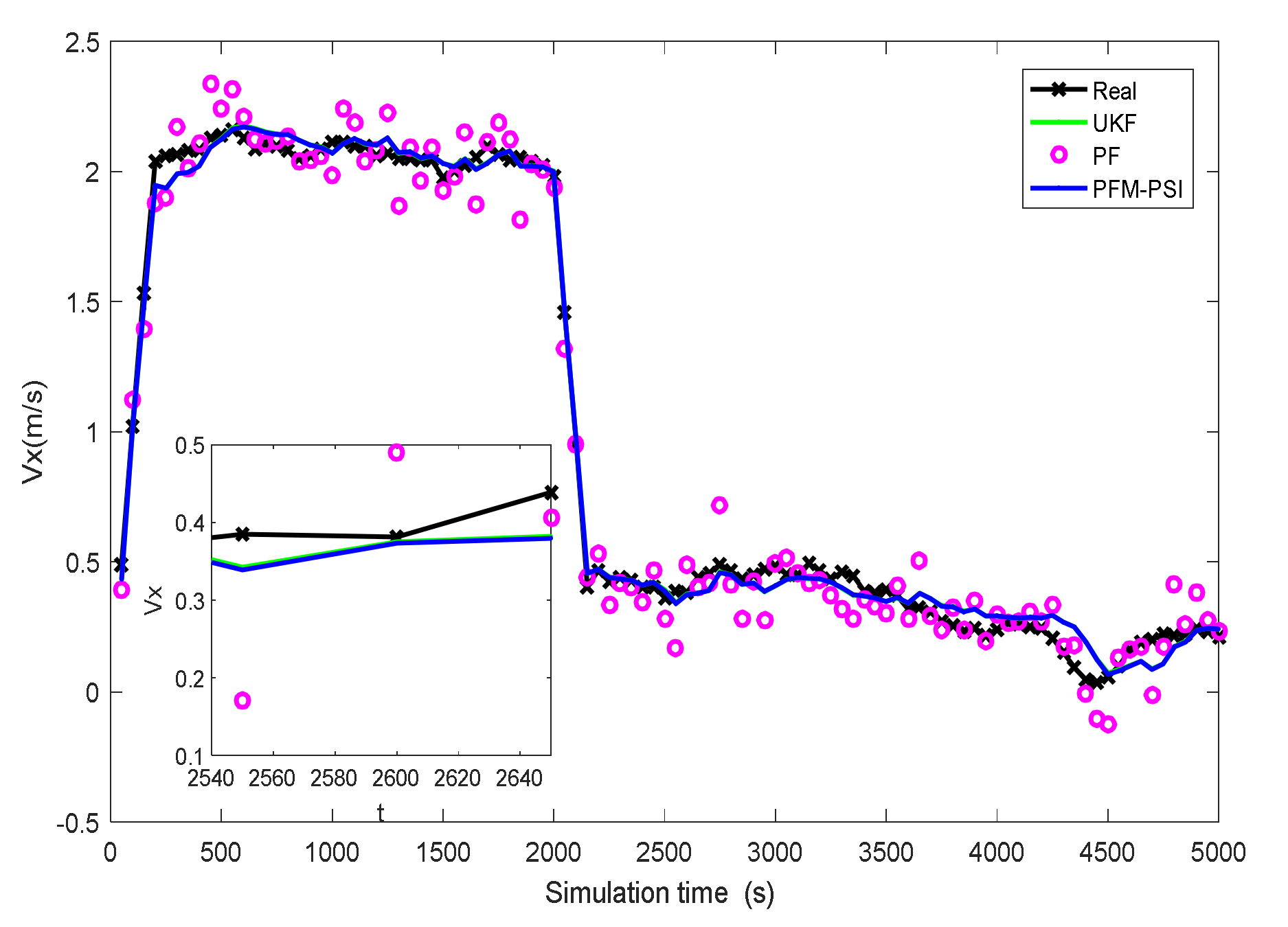
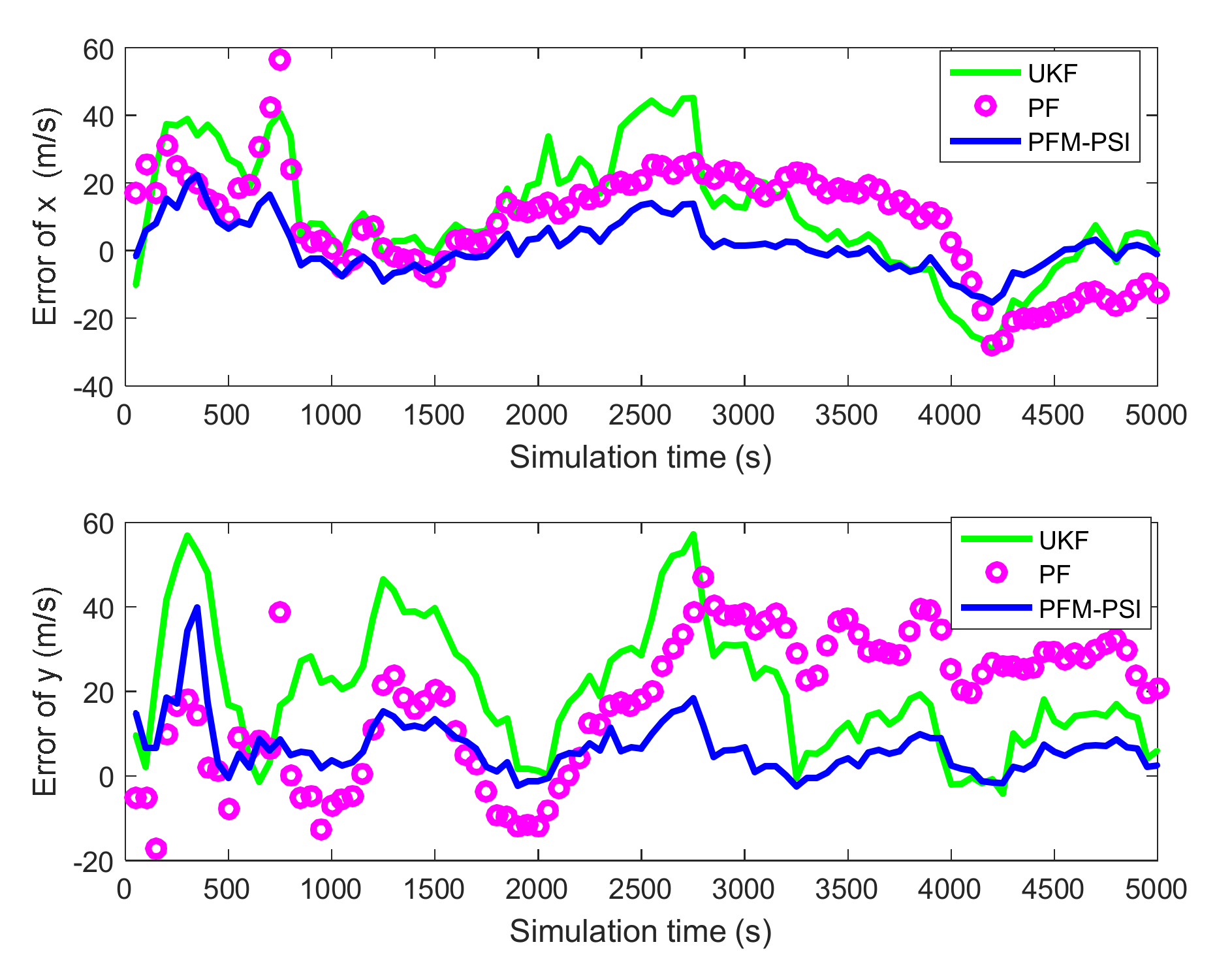
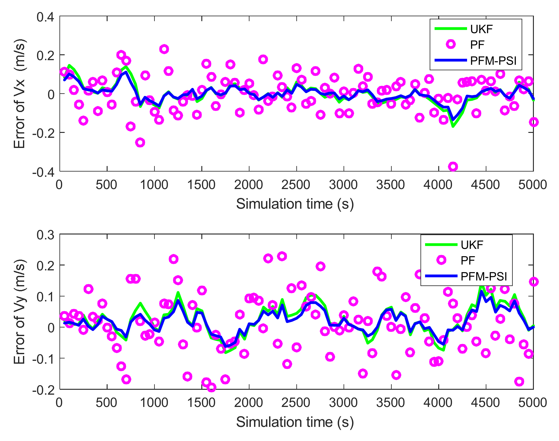
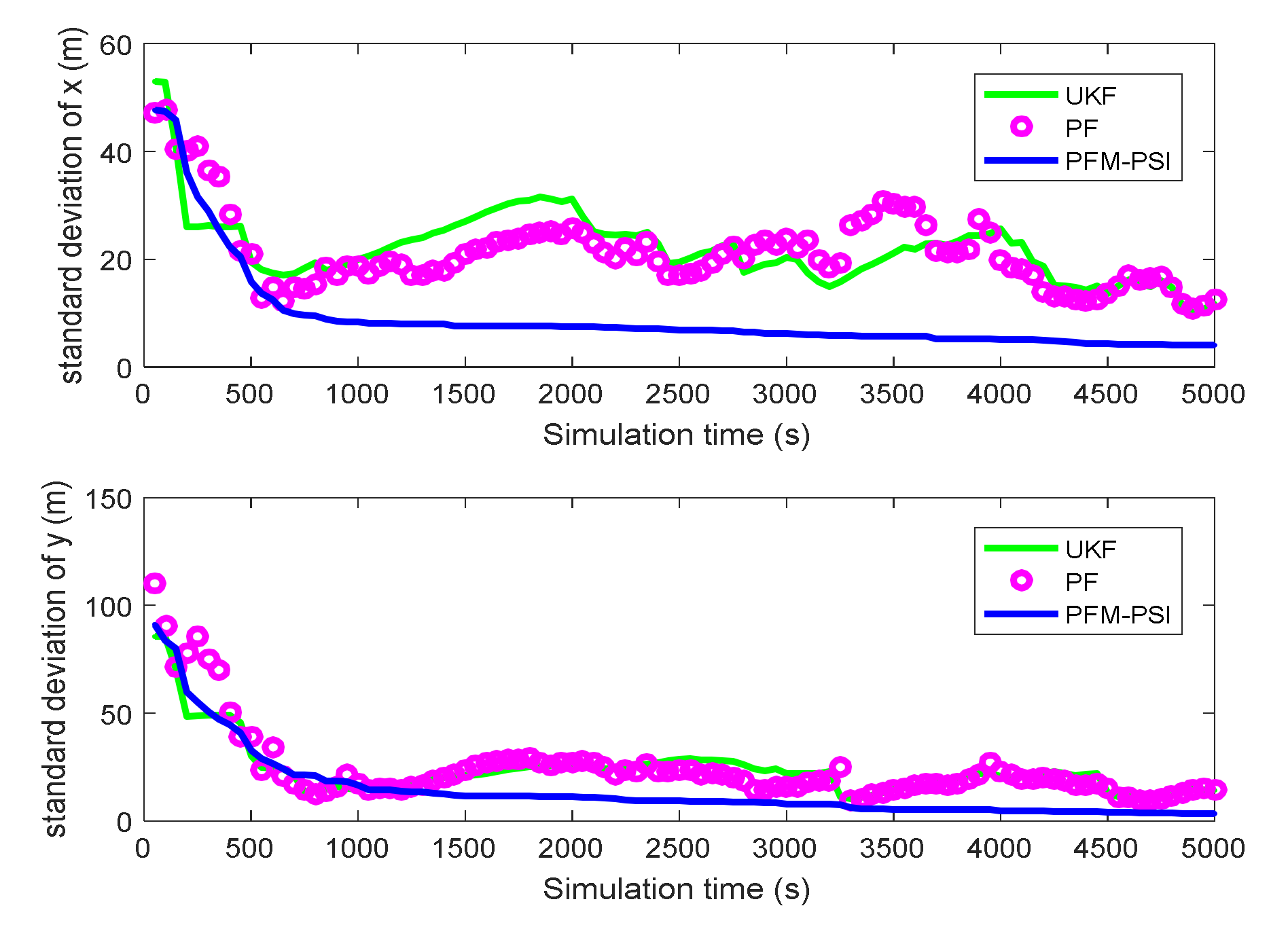
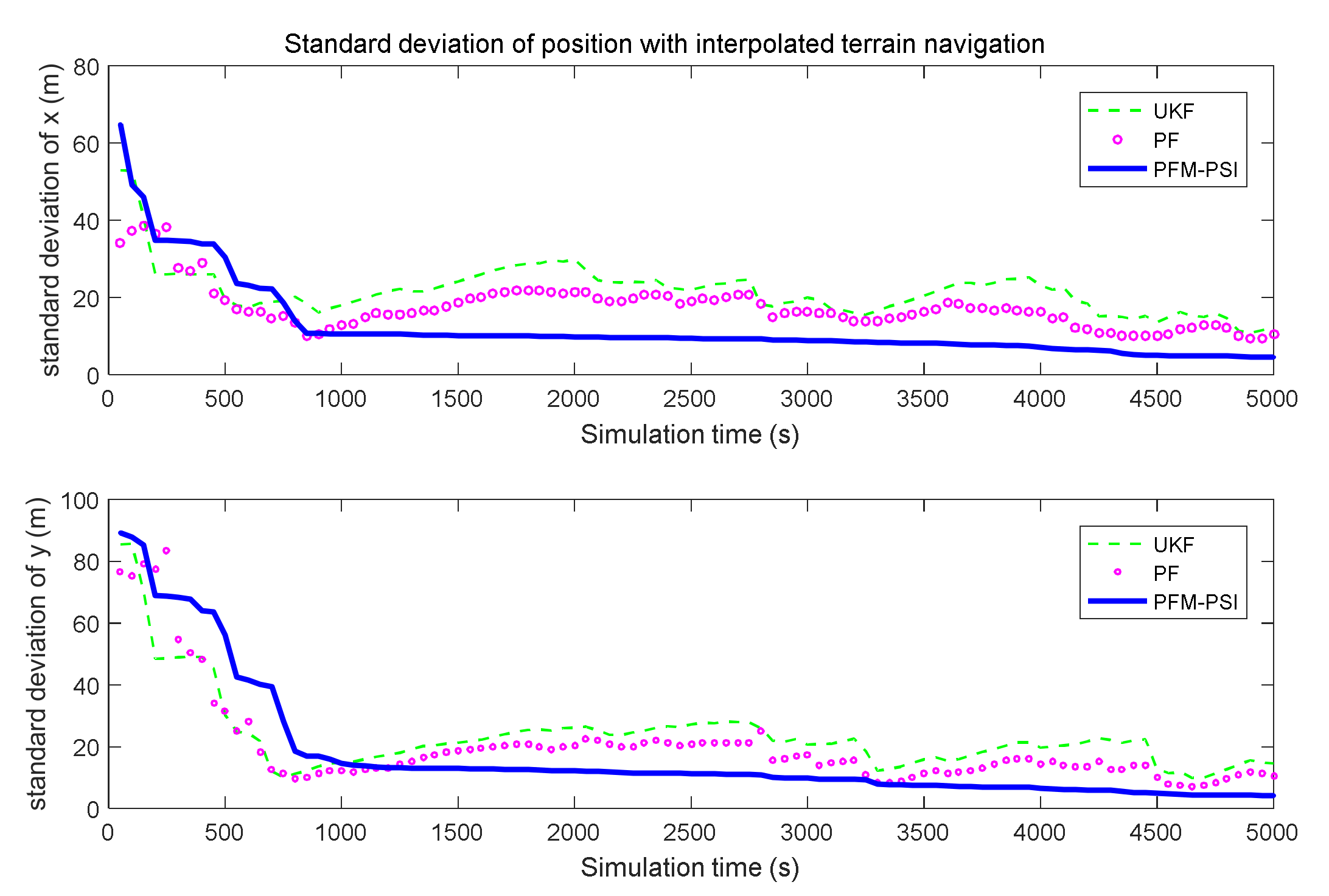
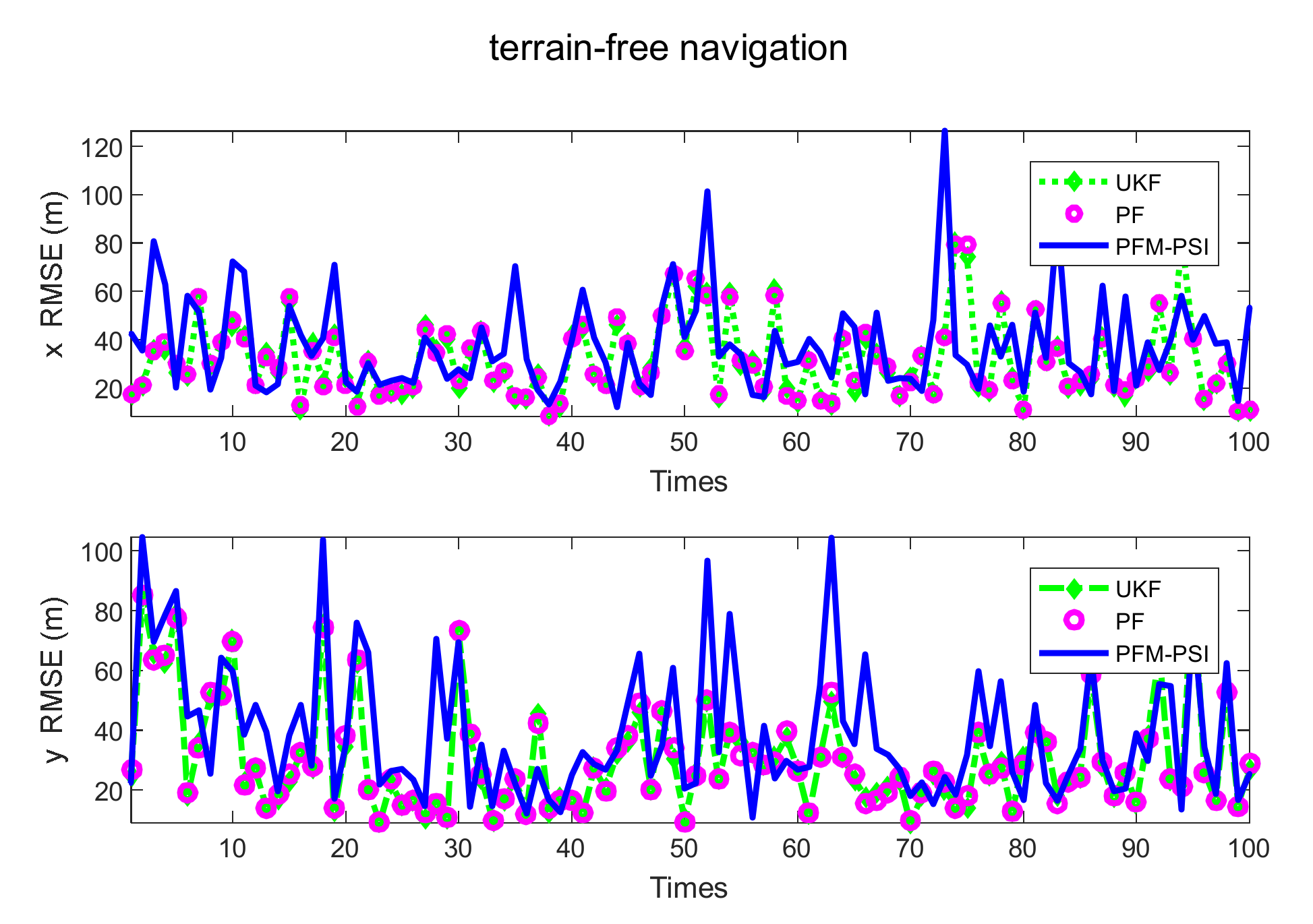
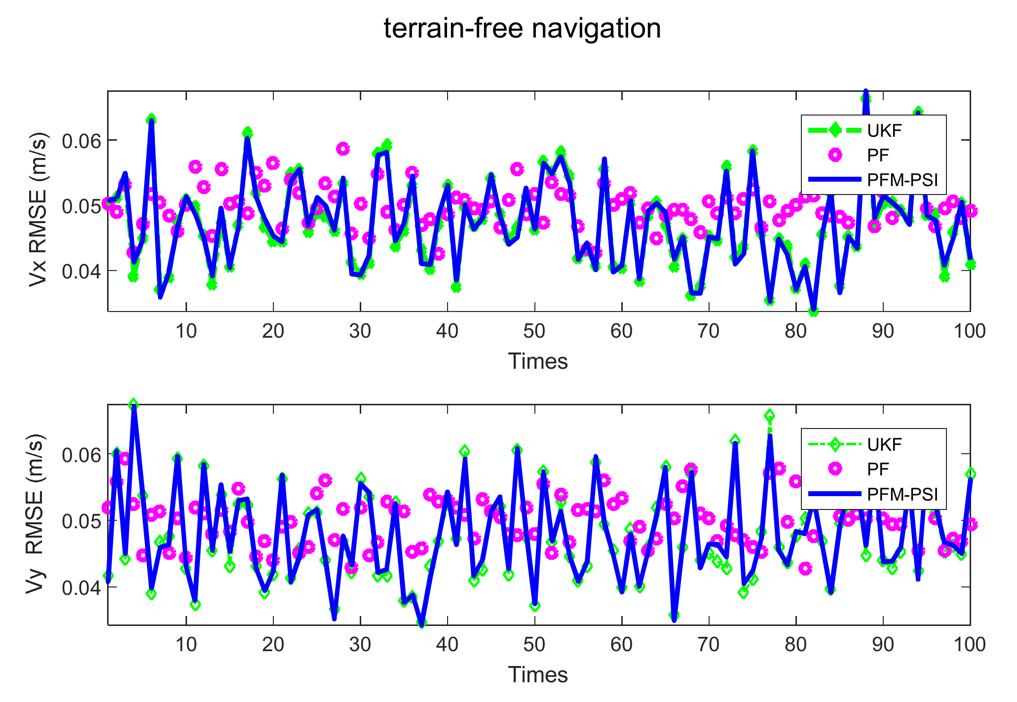
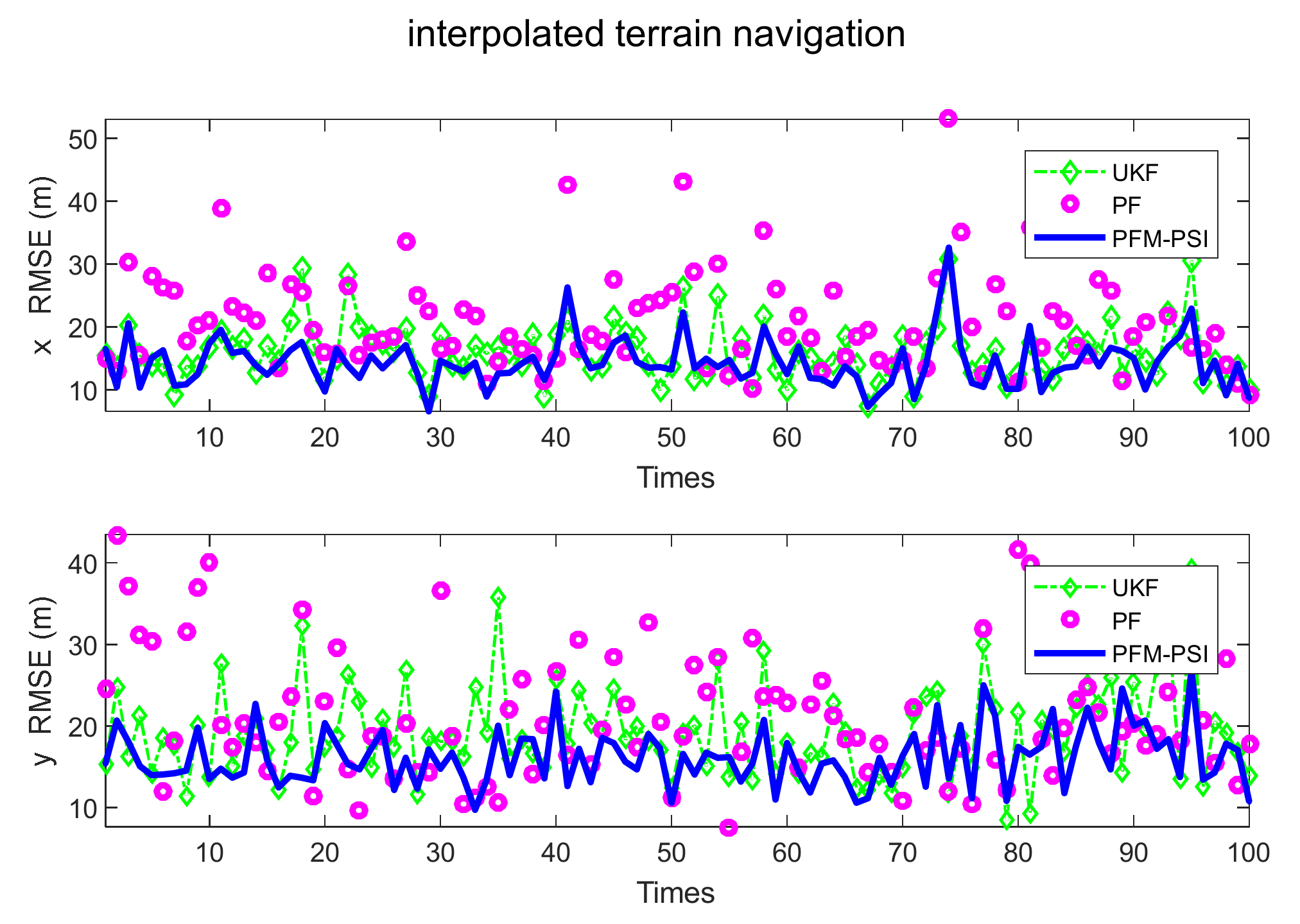
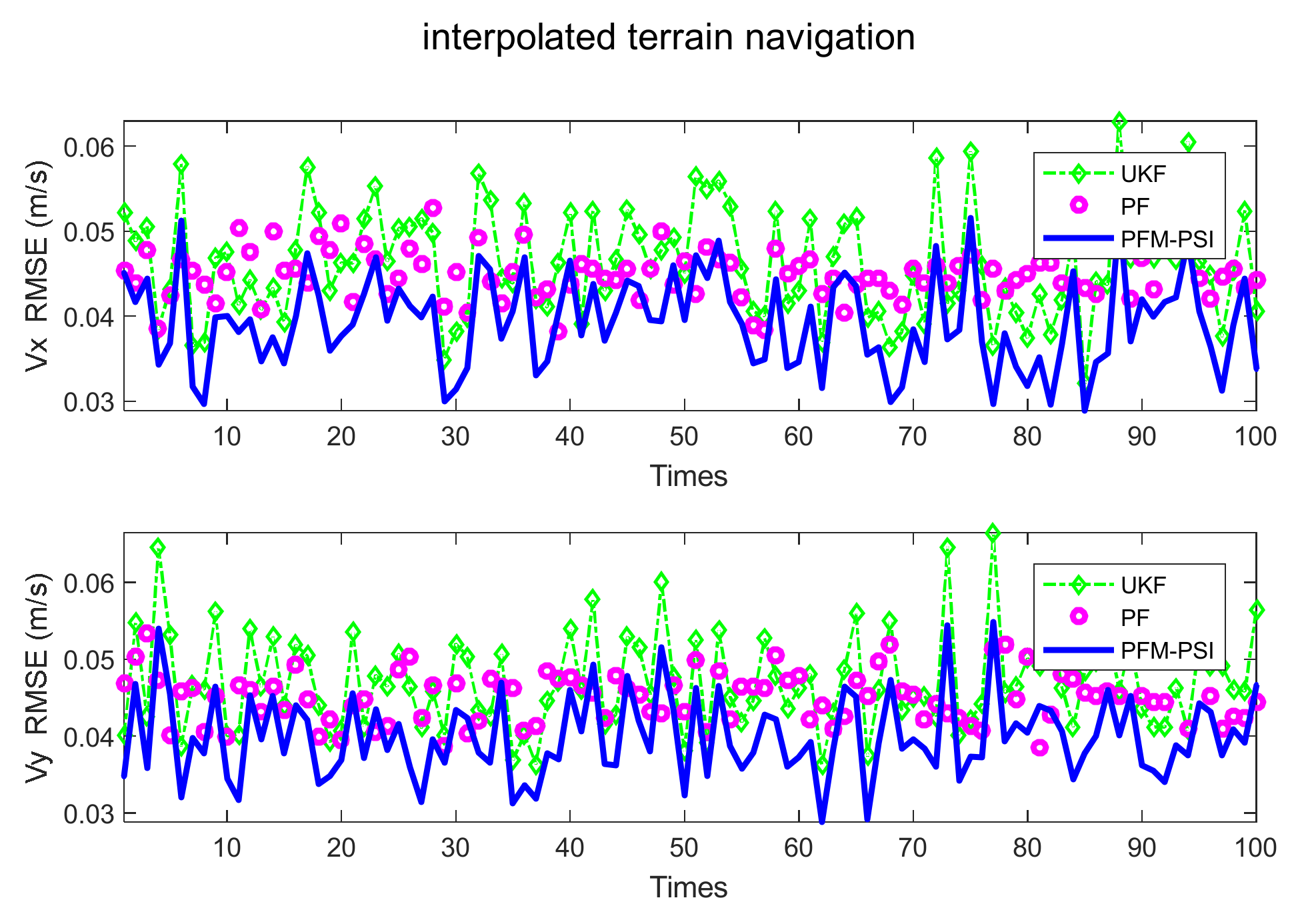
4.2. Example 2: State Estimation Model in Underwater Navigation

In this section, a nonlinear system in underwater navigation is given by References [29,30], which is described as follows:
State vector: X t = x t y t v x t v y t T .
Control vector: u t = ψ t a t T .
Measurement vector: z t = v x t v y t h r t + h t T .
Underwater navigation state estimation model:
X ˙ t = f x t , u t , w t = v x t c o s ψ t v y t s i n ψ t v y t c o s ψ t + v x t s i n ψ t a t c o s ψ t a t s i n ψ t + w x w y w v x w v y
z k = h X t k + e k = v x k v y k h d x t k , y t k + e v x e v y e h
where e = e v x , e v y , e h T , w = w x , w y , w v x , w v y T are, respectively, described as the measurement noise of the measurement equation and the process noise of the state equation. Zero mean white noise and the covariance matrix are, respectively, Q and R . h d x t , y t is expressed as a non-linear function.
Having set the initial state x0 = [2000 m; 18,000 m; 0.5 m/s; 0 m/s], the filter sampling time interval is Δ T = 1 s , the running time is 5000 s, the number of particles in the particle filter is 1000, and the number of orthogonal complex exponential basis functions is 10.
For the three non-linear filtering methods of UKF, PF and PFM-PSI (Projection Filter Method based on Projection Symmetric Interval), the terrain navigation in the experiment is displayed by using the interpolation method in Reference [25] to solve the terrain function. The state estimation results based on UKF, PF and PFM-PSI are shown in Figure 5, Figure 6, Figure 7, Figure 8, Figure 9, Figure 10, Figure 11, Figure 12, Figure 13, Figure 14, Figure 15, Figure 16 and Figure 17.
The real points in the experiment are generated by random numbers, and the results obtained from each simulation will be different. Therefore, the estimation accuracy of the verification algorithm is obtained by the statistical root mean square error (RMSE), which is defined as:
R = 1 S T i = 1 S T k = 1 t i m e s S k Y k 2 t i m e s
where R represents RMSE and Y k represents the estimated location information. the number of simulation experiments is S T = 100 , the simulation results are shown in Figure 18, Figure 19, Figure 20 and Figure 21.
In Figure 5, the true trajectory of a target can be viewed. The control vector with noise and the measured terrain profile are plotted in Figure 6 and Figure 7. Figure 8, Figure 9, Figure 10, Figure 11, Figure 12, Figure 13, Figure 14, Figure 15, Figure 16 and Figure 17 show the estimated trajectories, estimated mean and estimated standard deviation of state based on UKF, PF and PFM-PSI. We will give the performance output of PFM-PSI. Having compared the true state trajectory, estimated means and estimated standard deviation executed by UKF, PF and PFM-PSI, PFM-PSI is better than the other algorithms. These numerical experiment results show that the effectiveness of PFM-PSI is confirmed. Compare the true state trajectory and the conditional means of the trajectories executed by UKF, PF and PFM-PSI. Obviously, for a nonlinear system, the numerical experiment results show the feasibility and effectiveness of the novel nonlinear state estimation filter algorithm based on PFM.
The position RMSE and velocity RMSE of state can be plotted without terrain navigation in Figure 18 and Figure 19, and they can be plotted with interpolated terrain navigation in Figure 20 and Figure 21. Comparing position RMSE and velocity RMSE between terrain-free navigation and interpolation terrain navigation, the estimation accuracy of the three algorithms with interpolation terrain navigation is better. Compared with UKF and PF, PFM-PSI is significantly better than others, and the three algorithms are better with interpolated terrain navigation. In short, the estimation accuracy of PFM-PSI is obviously better than UKF and PF.
It can be seen from Figure 5, Figure 6, Figure 7, Figure 8, Figure 9, Figure 10, Figure 11, Figure 12, Figure 13, Figure 14, Figure 15, Figure 16, Figure 17, Figure 18, Figure 19, Figure 20 and Figure 21 that the PFM-PSI has better performance to obtain state estimation information in NLSs, so the PFM-PSI can estimate the PDF of state in the nonlinear non-gaussian systems. These all explain that PFM-PSI can improve the state estimation accuracy in Figure 5, Figure 6, Figure 7, Figure 8, Figure 9, Figure 10, Figure 11, Figure 12, Figure 13, Figure 14, Figure 15, Figure 16 and Figure 17. Although the PFM-PSI estimation accuracy is better, it does not quickly converge to the true state information in the NLSs, which also shows that the estimation accuracy of the PF is slightly lower than the PFM-PSI. In addition, Figure 6, Figure 7, Figure 8, Figure 9, Figure 10, Figure 11, Figure 12, Figure 13, Figure 14, Figure 15, Figure 16, Figure 17 and Figure 18 show that PFM-PSI needs to iteratively estimate state information with discrete time. This is consistent with the theoretical analysis in Section 3.
As to the efficiency, the CPU time for the PFM-PSI algorithm is 25.257 s for Times = 5000 s. Thus, for each time step, it only costs 0.005 s, and the calculation speed is much faster than the update time of 1 s. The CPU time for the PF algorithm is 31.100 s for Times = 5000 s. The CPU time for the UKF algorithm is 65.6224 s for Times = 5000 s. Obviously, the calculation speed of PFM-PSI is faster than that of PF and UKF.
Table 1 shows the mean RMSE 100 times in filtering simulations of the state estimation model. The PFM has a lower RMSE than the UKF and PF in Table 1. Having compared interpolated terrain navigation and terrain-free navigation, PFM-PSI performance is better with terrain navigation. Compared with the UKF and PF, obviously, the performance of PFM-PSI is better than PF and UKF shown in Table 1.

5. Conclusions

The effectiveness of a PFM-based projection symmetric interval in the state estimation approach to NLSs has been demonstrated in this paper. The main principle of the filter estimator is to apply a set of basis functions to iteratively calculate parameters of the prior PDF and posterior PDF based on the Fokker–Planck equation method and the Bayesian equation. In addition, a detailed theoretical derivation process is given in this paper, which mainly includes two parts: a status update and a measurement update. By taking two simple examples, we find that the PFM filter estimation performance is better than the UKF and PF methods. It can be applied to deal with output data from sensors with complex nonlinear systems, especially to solve the problem of high-dimensional state estimation. Compared with UKF and PF, the performance of PFM is significantly improved, the calculation speed is slightly faster, and the calculation complexity is lower. Although PFM gives a highly accurate approximate solution at each time step, to choose a scaling factor is not easy for arbitrary functions. We expect to find more robust ways to obtain the approximate solution for offline data. These problems will be further resolved in our future work.

Author Contributions

Writing—original draft preparation, L.C.; supervision and project administration, S.M.; software and funding acquisition F.F., X.X.; methodology, Y.Z.; investigation, Z.Z. All authors have read and agreed to the published version of the manuscript.

Funding

This work has been supported by the National Natural Science Foundation of China (grant number 51275363), the Natural Science Foundation of Hubei Province (grant number 2020CFB389), and Hubei Provincial Department of Education Science and Technology Research Project (grant number Q20201708).

Institutional Review Board Statement

Not applicable.

Informed Consent Statement

Not applicable.

Data Availability Statement

The study did not report any data.

Conflicts of Interest

The authors declare that they have no conflict of interest to this work. We declare that we do not have any commercial or associative interest that represents a conflict of interest in connection with the work submitted.

References

  1. Shang, J.; Chen, T. Optimal stealthy integrity attacks on remote state estimation: The maximum utilization of historical data. Automatica 2021, 128, 109555. [Google Scholar] [CrossRef]
  2. Gu, Y.; Lo, A.; Niemegeers, I. A survey of indoor positioning systems for wireless personal networks. IEEE Commun. Surv. Tutor. 2009, 11, 13–32. [Google Scholar] [CrossRef] [Green Version]
  3. Zhao, Y.; Chen, L.; Ma, Y. An FEM-based State Estimation Approach to Nonlinear Hybrid Positioning Systems. Math. Probl. Eng. 2013, 2013, 165–195. [Google Scholar] [CrossRef] [Green Version]
  4. Kalman, R.E. A New Approach to Linear Filtering and Prediction Problems. Trans. ASME J. Basic Eng. 1960, 82, 34–35. [Google Scholar] [CrossRef] [Green Version]
  5. Kalman, R.E.; Bucy, R.S. New Results in Linear Filtering and Prediction Theory. Trans. ASME J. Basic Eng. 1961, 83, 95–108. [Google Scholar] [CrossRef]
  6. Kandepu, R.; Foss, B.; Imsland, L. Applying the unscented Kalman filter for nonlinear state estimation. J. Process. Control. 2008, 18, 753–768. [Google Scholar] [CrossRef]
  7. Bucy, R.S.; Senne, K.D. Digital synthesis of nonlinear filters. Automatica 1971, 7, 287–298. [Google Scholar] [CrossRef]
  8. Kushner, H.J. Dynamical Equations for Optimal Nonlinear Filter. J. Differ. Equ. 1967, 3, 179–190. [Google Scholar] [CrossRef] [Green Version]
  9. Faruqi, F.A.; Tumer, K.J. Non-Linear Mathematical Model for Iniegrated Global Positioning/Inertial Navigation System. Appl. Math. Comput. 2000, 115, 213–227. [Google Scholar]
  10. Simon, J.; Durrant-Whyte, H.F. Process models for the high-speed navigation of road vehicles. In Proceedings of the IEEE International Conference on Robotics and Automation, Nagoya, Japan, 21–27 May 1995; pp. 101–105. [Google Scholar]
  11. Gordon, N.J.; Salmond, D.J.; Smith, A.F.M. Novel approach to nonlinearnon-Gaussian Bayesian state estimation. IEE Proc. Part F: Radar Signal Process. 1993, 140, 107–113. [Google Scholar]
  12. Pitt, M.K.; Shephard, N. Filtering Via Simulation: Auxiliary Particle Filters. J. Am. Stat. Assoc. 1999, 94, 590–591. [Google Scholar] [CrossRef]
  13. Li, X.; Gao, W.; Zhang, J. A Novel Hybrid Unscented Particle Filter based on Firefly Algorithm for Tightly-Coupled Stereo Visual-Inertial Vehicle Positioning. J. Navig. 2020, 73, 613–627. [Google Scholar] [CrossRef]
  14. Kotecha, J.H.; Djuric, P.M. Gaussian particle filtering. IEEE Trans. Signal Process. 2003, 51, 2592–2601. [Google Scholar] [CrossRef] [Green Version]
  15. Ye, Z.; Wang, T.; Wen, Q.; Zhang, X. Improved rao-blackwellised particle filter based on randomly weighted particle swarm optimization. Comput. Electr. Eng. 2018, 71, 477–484. [Google Scholar]
  16. Ann, C.B.; William, E.S. Bayesian Estimation of Multivariate Location Parameters. Handb. Stat. 2005, 25, 221–244. [Google Scholar]
  17. Nidhan, C.; Subhashis, G.; Anindy, R.; William, E.S. Bayesian Methods for Function Estimation. Handb. Stat. 2005, 25, 373–414. [Google Scholar]
  18. Patwardhan, S.C.; Narasimhan, S.; Jagadeesan, P.; Gopaluni, B.; Shah, S.L. Nonlinear Bayesian state estimation: A review of recent developments. Control. Eng. Pract. 2012, 20, 933–953. [Google Scholar] [CrossRef]
  19. Xu, H.; Xie, W.; Yuan, H.; Duan, K.; Liu, W.; Wang, Y. Fixed point iteration gaussian sum filtering estimator whith unknown time varying non gaussian measurement noise. Signal Process. 2018, 153, 132–142. [Google Scholar] [CrossRef]
  20. Zhang, Y.; Wu, Z.; Li, N.; Chambers, J. A novel adaptive kalman filter with inaccurate process and measurement noise covariance matrices. IEEE Trans. Automat. Contr. 2018, 63, 594–601. [Google Scholar]
  21. Park, S.; Hwang, J.; Kim, E.; Kang, H.J. A new evolutionary particle filter for the prevention of sample impoverishment. IEEE Trans. Evol. Comput. 2009, 13, 801–809. [Google Scholar] [CrossRef]
  22. Beard, R.; Gunther, J.; Lawton, J.; Stirling, W. Nonlinear projection filter based on galerkin approximation. J. Guid. Control. Dyn. 1999, 22, 258–266. [Google Scholar] [CrossRef]
  23. Lemos, J.M.; Costa, B.A.; Rocha, C. A Fokker-Planck approach to joint state-parameter estimation. IFAC-PapersOnLine 2018, 51, 389–394. [Google Scholar] [CrossRef]
  24. Barbara, K.; Barbara, P. Parameter estimation in SDEs via the Fokker–Planck equation: Likelihood function and adjoint based gradient computation. J. Math. Anal. Appl. 2018, 465, 872–884. [Google Scholar]
  25. Hosseiny, A.; Jaberipur, G. Complex exponential functions: A high-precision hardware realization. Integration 2020, 73, 18–29. [Google Scholar] [CrossRef]
  26. Hatamzadeh-Varmazyar, S.; Masouri, Z.; Babolian, E. Numerical method for solving arbitrary linear differential equations using a set of orthogonal basis functions and operational matrix. Appl. Math. Model. 2016, 40, 233–253. [Google Scholar] [CrossRef]
  27. Luo, X.; Yau, S.S.-T. Hermite Spectral Method with Hyperbolic Cross Approximations to High-Dimensional Parabolic PDEs. SIAM J. Numer. Anal. 2013, 51, 3186–3212. [Google Scholar] [CrossRef] [Green Version]
  28. Lathi, B.P. Linear Systems and Signals, 2nd ed.; Oxford University Press: New York, NY, USA, 2005; pp. 55–75. [Google Scholar]
  29. Anonsen, S.K.B. Advances in Terrain Aided Navigation for Underwater Vehicles. Ph.D. Thesis, Norwegian University of Science and Technology, Trondheim, Norway, 2010. [Google Scholar]
  30. Liu, X.; Fang, H.; Xiong, Z.; Xu, N. Multi-step-ahead Time Series Prediction based on LSSVR using UKF with Sliding-Windows. J. Xinyang Norm. Univ. Nat. Sci. Ed. 2019, 32, 320–326. [Google Scholar]
Figure 1. Flowchart of the estimator based on PFM.
Symmetry 13 01715 g001
Figure 2. Simulation results based on PFM–PSI and real solution.
Symmetry 13 01715 g002
Figure 3. Estimated error based on PFM–PSI.
Symmetry 13 01715 g003
Figure 4. Estimated RMS based on PFM–PSI.
Symmetry 13 01715 g004
Figure 5. True trajectory viewed.
Symmetry 13 01715 g005
Figure 6. Control vector with noise in one simulation.
Symmetry 13 01715 g006
Figure 7. Measured terrain profile.
Symmetry 13 01715 g007
Figure 8. Estimated trajectories based on UKF, PF and PFM-PSI without terrain navigation.
Symmetry 13 01715 g008
Figure 9. Estimated trajectories based on UKF, PF and PFM–PSI with interpolated terrain navigation.
Symmetry 13 01715 g009
Figure 10. Estimated mean of x based on UKF, PF and PFM–PSI.
Symmetry 13 01715 g010
Figure 11. Estimated mean of y based on UKF, PF and PFM–PSI.
Symmetry 13 01715 g011
Figure 12. Estimated mean of Vx based on UKF, PF and PFM-PSI.
Symmetry 13 01715 g012
Figure 13. Estimated mean of Vy based on UKF, PF and PFM–PSI.
Symmetry 13 01715 g013
Figure 14. Estimated error of position based on UKF, PF and PFM–PSI.
Symmetry 13 01715 g014
Figure 15. Estimated error of velocity based on UKF, PF and PFM–PSI.
Symmetry 13 01715 g015
Figure 16. Estimated standard deviation based on UKF, PF and PFM–PSI.
Symmetry 13 01715 g016
Figure 17. Estimated standard deviation of position with interpolated terrain navigation.
Symmetry 13 01715 g017
Figure 18. Position RMSE of three methods 100 times without terrain navigation.
Symmetry 13 01715 g018
Figure 19. Velocity RMSE of three methods 100 times without terrain navigation.
Symmetry 13 01715 g019
Figure 20. RMSE of position based on UKF, PF and PFM–PSI with interpolated terrain navigation.
Symmetry 13 01715 g020
Figure 21. RMSE of speed based on UKF, PF and PFM–PSI with interpolated terrain navigation.
Symmetry 13 01715 g021
Table 1. Mean RMSE 100 times in filtering simulations of state estimation model.
Title 1Title 2Title 3Title 4Title 4
UKF without terrain navigation
UKF with interpolated terrain navigation
42.797148.64310.04820.0475
24.387823.23410.04860.0484
PF without terrain navigation
PF with interpolated terrain navigation
42.797148.64310.04820.0475
13.993113.95900.04600.0454
PFM-PSI without terrain navigation
PFM-PSI with interpolated terrain navigation
23.637423.05740.04830.0479
13.852114.38150.04600.0451
Publisher’s Note: MDPI stays neutral with regard to jurisdictional claims in published maps and institutional affiliations.

