A Novel Underdetermined Blind Source Separation Method Based on OPTICS and Subspace Projection

Abstract

In recent years, the problem of underdetermined blind source separation (UBSS) has become a research hotspot due to its practical potential. This paper presents a novel method to solve the problem of UBSS, which mainly includes the following three steps: Single source points (SSPs) are first screened out using the principal component analysis (PCA) approach, which is based on the statistical features of signal time-frequency (TF) points. Second, a mixing matrix estimation method is proposed that combines Ordering Points To Identify the Clustering Structure (OPTICS) with an improved potential function to directly detect the number of source signals, remove noise points, and accurately calculate the mixing matrix vector; it is independent of the input parameters and offers great accuracy and robustness. Finally, an improved subspace projection method is used for source signal recovery, and the upper limit for the number of active sources at each mixed signal is increased from $m-1$ to m. The unmixing process of the proposed algorithm is symmetrical to the actual signal mixing process, allowing it to accurately estimate the mixing matrix and perform well in noisy environments. When compared to previous methods, the source signal recovery accuracy is improved. The method’s effectiveness is demonstrated by both theoretical and experimental results.

1. Introduction

Blind source separation (BSS) refers to the problem of separating source signals from the mixed observation signal when the signal mixing process is unknown [1,2,3]. In recent years, it has become a research focus, which is widely used in speech signal processing [4,5], biomedical signal processing [6,7], radar communication signal processing [8,9,10], fault diagnosis [11,12], and other fields. The number of observation sensors is often taken for granted in real applications, but the number of source signals is unknown and often exceeds the number of observation signals [13]. In this case, the BSS problem is known as underdetermined blind source separation (UBSS). Currently, the sparse component analysis (SCA) method is primarily employed to solve the UBSS problem [14,15], which usually involves two steps: mixing matrix estimation and source signal recovery.

Mixing matrix estimation is the premise of accurate signal recovery. The SCA-based mixing matrix estimate approach takes advantage of the signal’s linear clustering characteristic, which is sparse enough to solve the mixed vector. As the observed time domain signal often cannot meet the sparse condition, it is often transformed to the TF domain through short time Fourier transform (STFT) and Wigner–Ville Distibution (WVD) [16,17]. A method called degenerate unmixing estimation technique (DEUT) was proposed by Jourjine et al. [18], which requires speech signals to meet W-disjoint orthogonality in TF domain. Nevertheless, this condition is very strict for TF signals. In literature [19], a time–frequency ratio of mixtures (TIFROM) method was proposed, in which each source only needs to appear separately in a set of small adjacent TF windows. This method automatically determines the single-source TF region based on the variance of the TF field. Because the accuracy of the mixing matrix estimation is directly affected by the performance of the single source point (SSP) detection method, a large number of methods have emerged: those based on the angle difference of the real and imaginary parts of the TF points [20], sparse coding [21], the sparsity of source signals [22], etc. The selected SSPs are taken as the input of the clustering algorithm. The potential function method [23] is one of the earliest methods proposed in UBSS research, and it has strong robustness under the condition of strong noise or insufficient data samples, but it also has its limitations. For example, it can only be used in two-dimensional observation signals, and the number of source signals needs to be known. Recently, the application of combined clustering algorithm shows a growing trend. This is due to the fact that the combined approach can accurately estimate the column vector of the mixing matrix while determining the number of source signals, overcoming the limitations of a single clustering methods. DBSCAN-Hough employs density-based spatial clustering of application with noise (DBSCAN) to determine the number of clusters and Hough algorithm to locate the cluster center [24], and the AP-K algorithm uses affinity propagation (AP) clustering to determine the distribution of clusters and determines the initial point for K-means clustering [25]. In  [26], DBSCAN was used to perform cluster analysis to automatically find the number of clusters and the corresponding cluster center, and clustering by fast search and find of density peaks (CFSFDP) was utilized to determine the cluster center.

At present, the commonly used source signal recovery algorithms mainly rely on the sparsity of the signal in the transform domain. In order to find the sparse ${\ell }_0$-norm solution, the relaxation strategy is adopted to take the minimum ${\ell }_1$-norm solution as the effective approximation. The shortest path method proposed by Bofill [23] for two observed signals is the application of the minimum ${\ell }_1$-norm solution in the two-dimensional case. In [27], source signal reconstruction was transformed into a sparse minimization model based on ${\ell }_p$-norm, and the restored signal was solved by the iterative Lagrange multiplier method. The authors of [28] proposed the smoothed ${\ell }_0$-norm method to approximate the minimum ${\ell }_0$-norm, and the continuous Gaussian function was used to approximate the ${\ell }_0$-norm to obtain the sparse solution. In recent years, source signal reconstruction has been transformed into various optimization models, such as compressed sensing [29,30] and non-negative matrix factorization [31,32], all of which have achieved good results. Under the assumption that the number of simultaneous active source signals at any TF point does not exceed the number of observed signals, Aissa-el-Bey proposed a source signal recovery method based on subspace projection [33]. However, when the number of actual source signals is different from the assumed number, the estimated performance will degrade.

Based on the above analysis, it can be seen that the UBSS problem needs to be studied further, and a method with high accuracy, strong robustness, and a wide range of application needs to be proposed. Aiming at these objectives, this paper explores and proposes a novel method to solve the UBSS problem. The solution is to find the mixing matrix first, and then restore the signal, which is the symmetry of the actual signal mixing process. The SSPs are first screened out using principal component analysis (PCA), which is based on the short-term stationary properties of speech signals and the statistical characteristics of the TF points in the subinterval of the TF domain. Then, a mixing matrix estimation method combining OPTICS and potential function is proposed. OPTICS generates a decision graph based on the distribution density of SSPs regardless of the setting of parameters. It is easy to remove noise points and determine the number of source signals. The improved potential function can be used to determine the column vectors of the mixing matrix, which is suitable for multidimensional observation signals and has strong robustness. Finally, a method combining the subspace projection and the minimum ${\ell }_1$-norm of the number of source signals is used for source signal recovery.

The rest of this paper is organized as follows. In Section 2, the mathematical model for UBSS is introduced. In Section 3, the methods of SSP screening, mixing matrix estimation, and source signal recovery are introduced in detail. Section 4 gives the experimental results. The content and work of this paper are summarized in Section 5.

2. Mathematical Model of UBSS

In the time domain, the BSS model of underdetermined instantaneous mixing can be defined as

$$\mathbf{x}\left(t\right)=\left[\begin{array}{c}{x}_1\left(t\right)\\ x_2\left(t\right)\\ ⋮\\ x_m\left(t\right)\end{array}\right]=\left[\begin{array}{cccc}{a}_{11}& a_{12}& \dots & a_{1n}\\ a_{21}& a_{22}& \cdots & a_{2n}\\ ⋮& ⋮& \ddots & ⋮\\ a_{m1}& a_{m2}& \cdots & a_{mn}\end{array}\right]\left[\begin{array}{c}{s}_1\left(t\right)\\ s_2\left(t\right)\\ ⋮\\ s_n\left(t\right)\end{array}\right]=\mathbf{As}\left(t\right)t=1,2,\dots ,T$$

(1)

where $\mathbf{s}\left(t\right)={[s_1\left(t\right),s_2\left(t\right),\cdots ,s_n\left(t\right)]}^T$ represents n source signals, and $\mathbf{x}\left(t\right)=[x_1\left(t\right),x_2\left(t\right),$$\cdots ,x_m\left(t\right){]}^T$ represents m mixed signals. $\mathbf{A}=[{\mathbf{a}}_1,{\mathbf{a}}_2,\dots ,{\mathbf{a}}_n]\in {\mathbf{R}}^{m\times n}(m<n)$ is the unknown mixing matrix. The main purpose of UBSS is to accurately separate the source signal $\mathbf{s}\left(t\right)$ when only the observed signal $\mathbf{x}\left(t\right)$ is known. In order to ensure that the source signal can be separated, the mixing matrix needs to satisfy the following assumptions:

Assumption 1.

Any $m\times m$ submatrix of the mixing matrix $\mathbf{A}$ is full rank.

The solution of the UBSS depends on the sparsity of signals. Speech signals typically overlap in the time domain, and they do not meet the sparsity condition. As a result, the STFT is utilized to convert the signals into the TF domain for analysis and processing, and the transformed model is shown as follows:

$$\mathbf{X}(t,f)=\mathbf{AS}(t,f)$$

(2)

For signals in the TF domain, the following assumptions need to be met:

Assumption 2.

For each source signal $S_i(t,f)$, there is a TF region $(t,f)$ satisfying $|S_i(t,f)|$$\gg \left|S_j(t,f)\right|,j\in [1,n],j\ne i$, that is, the signal is sparse sufficiently.

For sufficiently sparse observed signals which satisfying assumption 2, there exists a certain TF region where only one signal dominates. The observation points in the region show linear clustering characteristics, as shown in Equation (3). The slope depends on the column vector ${[a_{i1},a_{i2},\dots ,a_{im}]}^T$. This property can be used to estimate the mixing matrix accurately.

$$\frac{x_1(t_i,f_j)}{a_{i1}}=\frac{x_2(t_i,f_j)}{a_{i2}}=\dots =\frac{x_m(t_i,f_j)}{a_{im}}$$

(3)

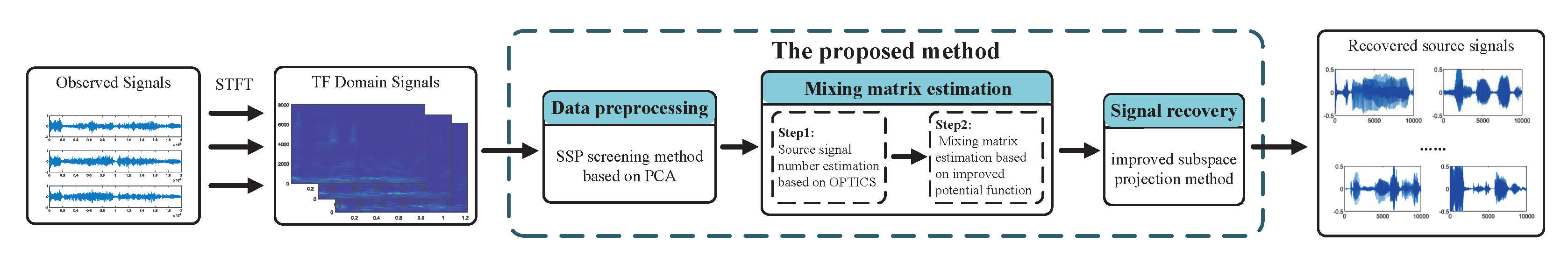
3. The Proposed Method

The method proposed in this paper includes three steps: SSP screening, mixing matrix estimation, and source signal recovery. The complete processing flow chart is shown in Figure 1:

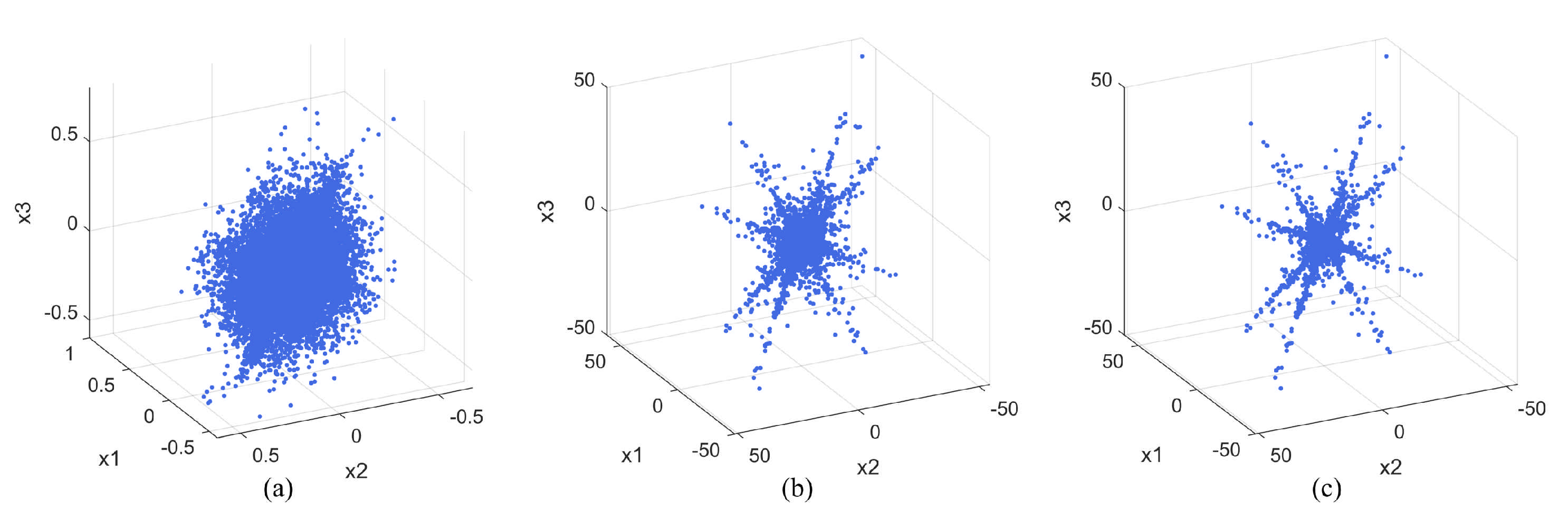
3.1. SSP Screening Method Based on PCA

After STFT, the time-domain observed signal $x_i$ is converted to the TF domain ${\mathrm{\Omega }}_i$. Divide ${\mathrm{\Omega }}_i$ into disjoint subintervals with time length $∆t_0$ and frequency length $∆f_0$, the TF points in subinterval $∆{\mathrm{\Omega }}_i$ can be expressed as

$$∆{\mathrm{\Omega }}_i=\left\{x_i(t,f)\right|t\in (k_1∆t_0,(k_1+1)∆t_0),f\in (k_2∆f_0,(k_2+1)∆f_0)\}$$

(4)

where $k_1,k_2\in \mathrm{Z}$. As the speech signal can often remain stable in a short time interval, the subinterval can be used as an independent unit, and PCA can be used for SSP screening. The processing steps of the algorithm are as follows.

Suppose a vector $\mathbf{X}(t,f)$ composed of observed signals from the same TF interval. Perform decentralized preprocessing first:

$$\mathbf{X}(t,f)\leftarrow \mathbf{X}(t,f)-E\left[\mathbf{X}\right(t,f\left)\right]$$

(5)

where $E\left[\mathbf{X}\right(t,f\left)\right]$ represents the average value of the observed signal, and the autocorrelation matrix of the mixed signal is

$$R_x=E\left[\mathbf{X}(t,f){\mathbf{X}}^H(t,f)\right]=E\left[\mathbf{AS}(t,f){\mathbf{S}}^H(t,f){\mathbf{A}}^H\right]=\mathbf{A}{R}_s{\mathbf{A}}^H$$

(6)

where ${[·]}^H$ is the conjugate transpose. Carry out the eigenvalue decomposition of $R_x$:

$$R_x=U\sum U^H$$

(7)

where $U=[{\mathbf{u}}_1,{\mathbf{u}}_2,\dots ,{\mathbf{u}}_m]$ is the unitary matrix composed of eigenvectors, ${\displaystyle \sum }=diag({\lambda }_1,{\lambda }_2,$$\dots ,{\lambda }_m)$ is a diagonal matrix, and the eigenvalues are assumed to be arranged in descending order ${\lambda }_1\ge {\lambda }_2\ge \dots \ge {\lambda }_m$. When the TF points in the subinterval $∆{\mathrm{\Omega }}_i$ are SSPs, $rank\left(R_x\right)=1$, then the eigenvalue satisfies

$$\left\{\begin{array}{c}{\lambda }_1\ne 0\hfill \\ {\lambda }_2,\dots ,{\lambda }_m=0\hfill \end{array}\right.$$

(8)

In this case, the autocorrelation matrix of mixed signals can be written as

$$R_x={\mathbf{a}}_{k}E\left[s_k{(t,f)}^2\right]{\mathbf{a}}_k^H={\mathbf{u}}_1{\lambda }_1{{\mathbf{u}}_1}^H$$

(9)

where $s_k(t,f)$ is the source signal, ${\mathbf{a}}_k$ is the mixing matrix column vector corresponding to $s_k(t,f)$, and ${\mathbf{u}}_1$ is the eigenvector corresponding to the eigenvalue ${\lambda }_1$. Therefore, the SSP interval can be screened by judging the value of the principal eigenvalue. Because of the existence of noise in practice, ${\lambda }_2,\dots ,{\lambda }_m=0$ is often difficult to be guaranteed, so the threshold $\phi$ is set to relax the conditions for SSP screening:

$$\frac{\left|{\lambda }_1\right|}{{\displaystyle \sum _{i=1}^m}\left|{\lambda }_i\right|}\ge \phi$$

(10)

where $\phi$ is a value close to 1, indicating that only one source signal is dominant in the region. The subinterval satisfying Equation (9) can be considered as the SSP interval.

3.2. Mixing Matrix Estimation

In this section, a mixing matrix estimation method based on the combination of OPTICS and improved potential function method is proposed. First, OPTICS generates the decision graph, determines the number of source signals, and eliminates the noise points. The cluster center, i.e., the mixing matrix vector, is then determined by calculating the local potential of observation points within the class.

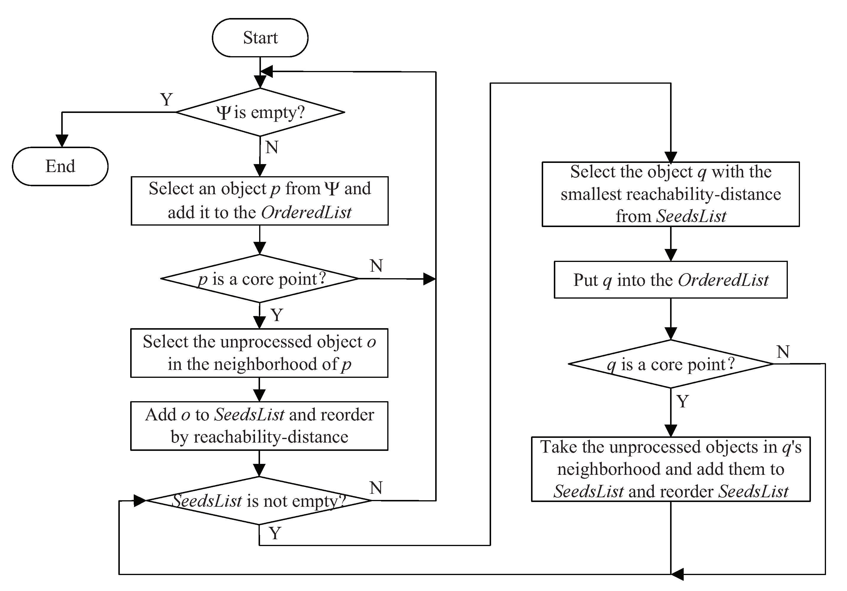
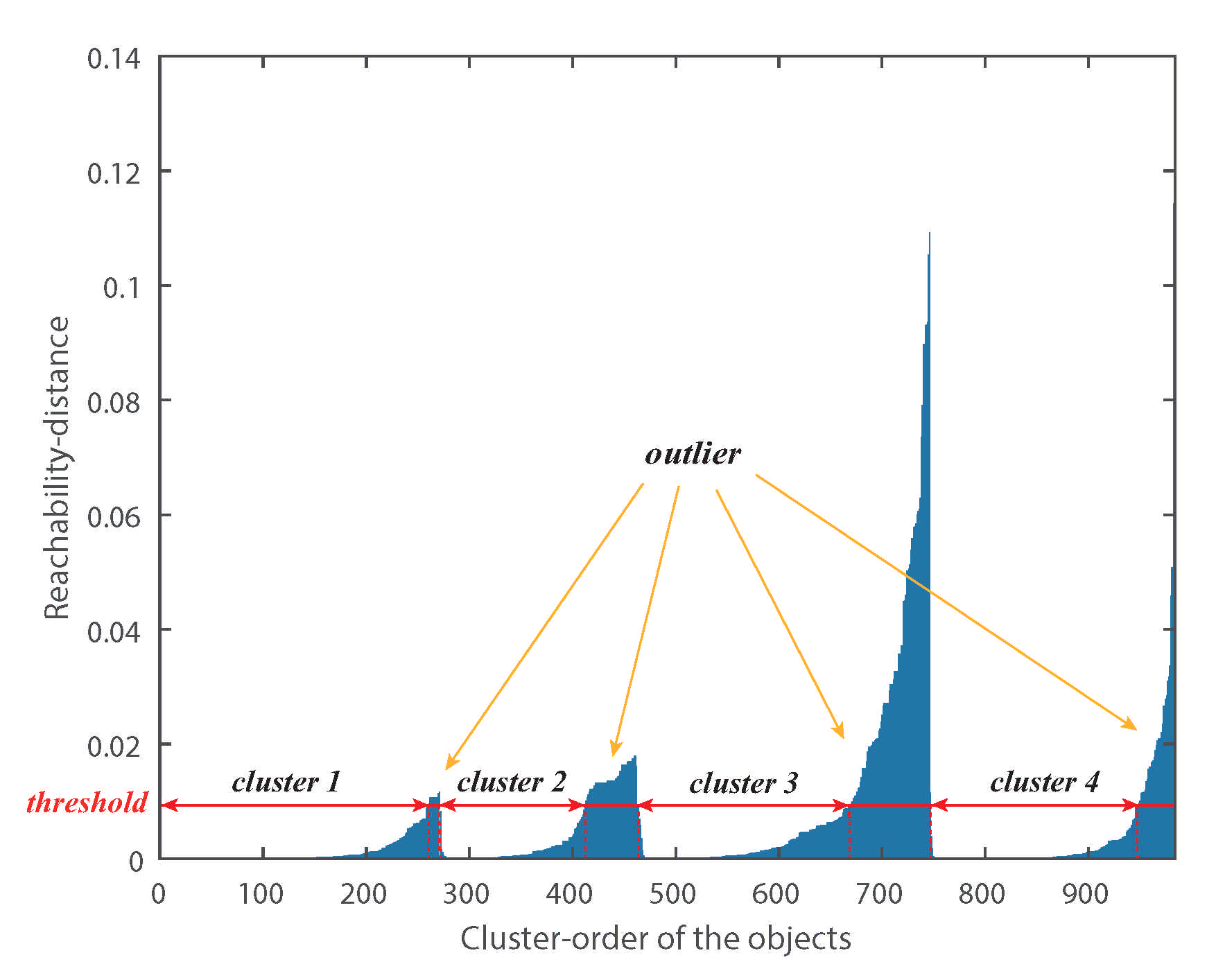
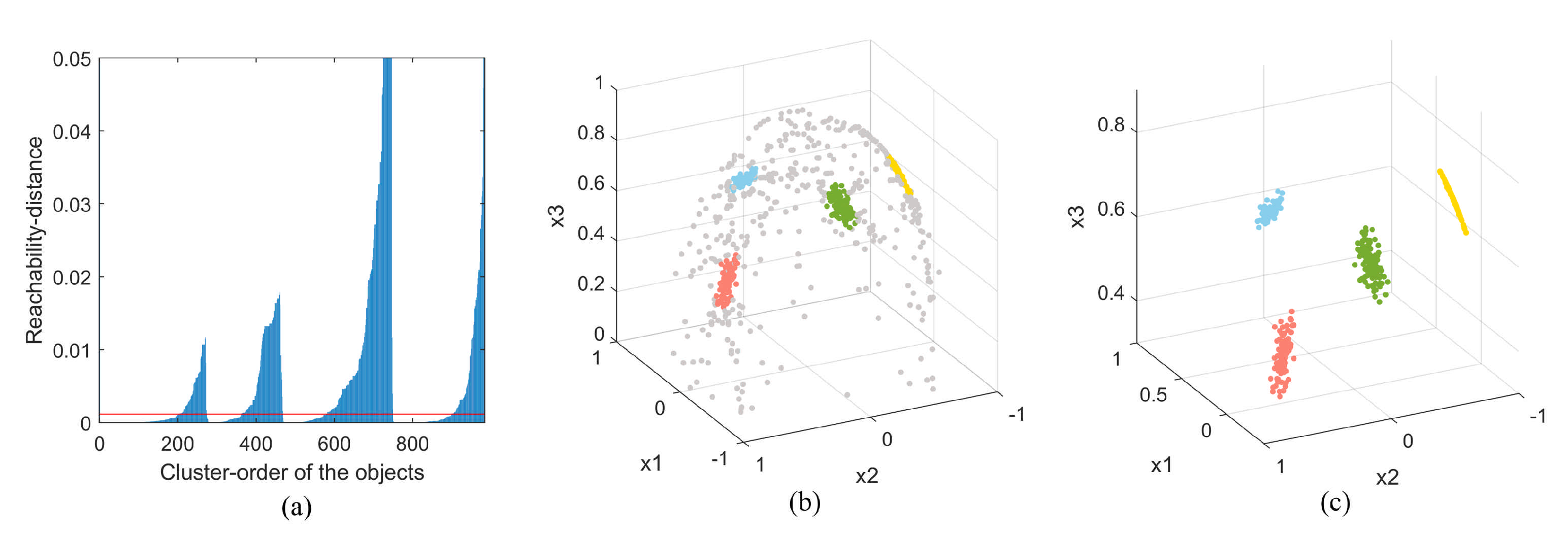
3.2.1. Source Signal Number Estimation Based on OPTICS

OPTICS is a clustering method based on data density, which can be regarded as an improvement based on DBSCAN [34]. DBSCAN needs to dynamically adjust parameters to adapt to the data distribution under different circumstances and getting the correct categorization, which limits its application. OPTICS calculates and stores the distance information of the sample points and sorts it in a way that produces an ordered list of the distribution of the sample data, reflecting the density structure within the data.

For any observation signal ${\mathbf{X}}_i(t,f)\in \mathrm{\Omega }$ in TF domain after SSP screening, it can be regarded as a point in m dimensional space. To ensure the effect of OPTICS, the low-energy points are first deleted, as shown in Equation (11). Then, use Equation (12) to normalize and project the remaining points. The projection process is to find the symmetry about the origin of the points on the negative semi-axis, which can make the data distribution more dense and facilitate the processing of the clustering method. Set a low energy threshold $\lambda$ and retain the points where the energy is greater than the threshold.

$$∥\mathbf{X}(t,f)∥\ge \lambda$$

(11)

$$\tilde{\mathbf{X}}(t,f)=sign\left(x_m(t,f)\right)\frac{\mathbf{X}(t,f)}{∥\mathbf{X}(t,f)∥}$$

(12)

The processed observation signal is regarded as a set of points distributed in space, denoting as $\mathrm{\Psi }=\{{\tilde{x}}_1,{\tilde{x}}_2,\dots ,{\tilde{x}}_l\}$. For each sample data point, OPTICS introduces two parameters: the neighborhood radius ($\epsilon$) and the number of sample points specified in the neighborhood ($MinPts$). Two definitions are given: core-distance and reachability-distance. In traditional OPTICS, the concepts of neighborhood radius, core-distance, and reachability-distance are all based on the Euclidean distance to measure the distribution of data. When solving the problem of UBSS, as the input data are the normalized observation signal, the angle between the data vectors can objectively reflect the density of the data compared to the Euclidean distance, so the distance in this paper is defined as

$$\phi (x_i,x_j)=1-〈x_i,x_j〉=1-\sum _{k=1}^n{x}_{ik}·x_{jk}$$

(13)

The relevant explanations for the remaining definitions are as follows:

Definition 1.

The calculation equation of the core-distance is as follows:

$$C{D}_{\epsilon ,MinPts}\left({\tilde{x}}_i\right)=\left\{\begin{array}{cc}UNDEFINED\hfill & Card\left(N_{\epsilon }\left({\tilde{x}}_i\right)\right)<MinPts\hfill \\ \phi ({\tilde{x}}_i,{\tilde{x}}_{MinPts})\hfill & Card\left(N_{\epsilon }\left({\tilde{x}}_i\right)\right)\ge MinPts\hfill \end{array}\right.$$

(14)

where $N_{\epsilon }\left({\tilde{x}}_i\right)$ represents the neighborhood with point ${\tilde{x}}_i$ as the center and ε as the radius.

$Card\left(N\right)$ is the number of elements contained in set N, and points satisfying $Card\left(N_{\epsilon }\left({\tilde{x}}_i\right)\right)$$\ge MinPts$ are called core objects. Equation (14) indicates that if ${\tilde{x}}_i$ is not the core point (the number of points in $\epsilon$ neighborhood is less than $MinPts$), then there is no core-distance. If ${\tilde{x}}_i$ is the core point and ${\epsilon }^{\prime }$ is the radius, it can just meet the requirement that the number of core points is $MinPts$, then ${\epsilon }^{\prime }$ is the core-distance.

Definition 2.

The calculation equation of the reachability-distance is as follows:

$$R{D}_{\epsilon ,MinPts}({\tilde{x}}_i,{\tilde{x}}_j)=\left\{\begin{array}{cc}UNDEFINED\hfill & Card\left(N_{\epsilon }\left({\tilde{x}}_i\right)\right)<MinPts\hfill \\ max(CD\left({\tilde{x}}_i\right),\phi ({\tilde{x}}_i,{\tilde{x}}_j))\hfill & Card\left(N_{\epsilon }\left({\tilde{x}}_i\right)\right)\ge MinPts\hfill \end{array}\right.$$

(15)

If ${\tilde{x}}_i$ is not the core point, there is no reachable distance. If ${\tilde{x}}_i$ is the core point and the distance between ${\tilde{x}}_j$ and ${\tilde{x}}_i$ is greater than the core-distance of ${\tilde{x}}_i$, the reachability-distance is $\phi ({\tilde{x}}_i,{\tilde{x}}_j)$. If the distance from ${\tilde{x}}_j$ to ${\tilde{x}}_i$ is less than or equal to the core-distance of ${\tilde{x}}_i$, then the reachability-distance is equal to the core-distance of ${\tilde{x}}_i$.

The specific steps for applying OPTICS to estimate the number of source signals are as follows:

Input: the observed signal point set $\mathrm{\Psi }$, radius of neighborhood $\epsilon$, minimum number of points in the neighborhood $MinPts$

• Create a result queue OrderedList, which is used to store processed points in the order of processing; create an ordered queue SeedsList, which is used to store the points that will be processed, and arranged in ascending order of reachable distance;
• If $\mathrm{\Psi }$ is not empty, select the core object p from the point set and add it to the OrderedList. Find the unprocessed objects in its neighborhood and put them in the SeedsList, and reorder SeedsList according to the reachability-distance. If $\mathrm{\Psi }$ is empty, the algorithm ends;
• If the SeedsList is not empty, select the first object (the object with the smallest reachability-distance) into the OrderedList; if the SeedsList is empty, go back to step 2;
• If object q is the core object, select the unprocessed objects in its neighborhood and put them in SeedsList. Then update the reachability-distance and sorting of the objects in SeedsList; If q is not a core object, return step 3;

The algorithm flow chart is shown in Figure 2.

Draw a graph for the observed signal points according to the processing order of the objects in the OrderedList, and take the reachability-distance as the ordinate. Clusters appear as valleys in the decision graph. The deeper the valleys are, the denser the data distribution is. The larger the reachability-distance is, the farther away the distribution of the points is from the center of the cluster, which can be regarded as outliers. According to the number of valleys in the figure, the number of cluster centers in the observed signals can be determined, that is, the number of source signals. Figure 3 shows the decision diagram of the OPTICS algorithm. Set the threshold value $\alpha$, as shown in Equation (16). The points where the reachability-distance exceeds the threshold value are regarded as outliers which need to be deleted.

$$\rho =\alpha ·(min\left\{Lmax\left(C{D}_{\epsilon ,MinPts}\left({\tilde{x}}_i\right)\right)\right\}-max\left\{Lmin\left(C{D}_{\epsilon ,MinPts}\left({\tilde{x}}_i\right)\right)\right\}){\tilde{x}}_i\in \mathrm{\Psi }$$

(16)

where $Lmax(·)$, $Lmin(·)$ represent the local maximum and local minimum, respectively.

3.2.2. Mixing Matrix Estimation Based on Improved Potential Function

Through OPTICS, outliers that affect the clustering effect are removed, and observation points are grouped into different clusters according to their density. In this section, an improved potential function method is used to calculate the local potential of the observation points within the cluster and determine the cluster center, which overcomes the shortcoming that the traditional potential function method cannot be applied to the high-dimensional observation signals and retains the advantage of its strong robustness.

Suppose that after OPTICS, the data are divided into r clusters, and the number of data in each cluster is $\{k_1,k_2,\dots ,k_r\}$. Assuming that for a certain cluster n, the number of data is $k_n$, then the local potential function of any element ${\mathbf{x}}_i^n$ in the cluster can be calculated as follows:

$$\mathrm{\Phi }\left({\mathbf{x}}_i^n\right)=\sum _{j=1}^{k_n}∥{\mathbf{x}}_i^n∥·f\left(\phi ({\mathbf{x}}_i^n,{\mathbf{x}}_j^n)\right)j,i\in \{1,2,\dots ,k_n\},j\ne i$$

(17)

The basis function $f(·)$ selects a piecewise function, and the equation is as follows:

$$f\left(\theta \right)=\left\{\begin{array}{cc}{e}^{\theta }-1\hfill & \theta \ge 0\hfill \\ 0\hfill & \theta <0\hfill \end{array}\right.$$

(18)

$\phi (·)$ is the cosine of the angle between any two vectors, and the smaller $\phi (·)$ is, the closer the two vectors are.

$$\phi (\mathbf{x},\mathbf{y})=\frac{\mathbf{x}·\mathbf{y}}{∥\mathbf{x}∥∥\mathbf{y}∥}$$

(19)

For a certain vector ${\mathbf{x}}_j^n$, the greater the number of vectors with less deviation from its direction is, the greater its local potential. In the case of the same deviation angle, the vector with high energy value has a greater contribution than low energy one.

3.3. Source Signal Recovery Based on the Improved Subspace Projection Method

According to the theory of subspace projection, in the linear instantaneous mixing model, for the observed signal $x_t(t,f)$ at a certain moment, it is assumed that the number of source signals simultaneously acting at this time is k, which, respectively, corresponds to the mixing vector ${\mathbf{a}}_1,\dots ,{\mathbf{a}}_k$, where $\{1,\dots ,k\}\in \{1,2,..,n\}$. The observed signal can be regarded as distributed in the subspace formed by the mixing vectors, $S_k=span({\mathbf{a}}_1,{\mathbf{a}}_2,\dots ,{\mathbf{a}}_k)$. The source signal recovery method based on subspace projection proposed in literature [33] assumes that the number of effective source signals at any TF point is strictly less than the number of mixed signals. In other words, if m observed signals exist, at most $m-1$ source signals can exist at any TF point.

When using this method, define the projection error matrix $Q_k$:

$$Q_k=I-{\mathbf{A}}_k{\left({\mathbf{A}}_k^H{\mathbf{A}}_k\right)}^{-1}{\mathbf{A}}_k^H$$

(20)

Assuming that the number of active source signals at any time is $k=m-1$, the active column vector of the mixing matrix at that TF point is determined by finding the smallest projection error:

$$\{{\mathbf{a}}_1,{\mathbf{a}}_2,\dots ,{\mathbf{a}}_k\}=argmin\left\{∥Q_k·x_t(t,f)∥\right|{\mathbf{A}}_k\}$$

(21)

When the actual number of source signals is $u(u<m-1)$, even if the projection error takes the minimum value, as in Equation (22), the estimation result will produce additional errors. This is due to the existence of interference in practice, and the ideal state of Equation (22) is difficult to achieve. When the number of estimated source signals is greater than the actual value, errors will be introduced into the estimation result, as shown in Equation (23). Therefore, it is necessary to accurately estimate the number of source signals at the TF points.

$$\begin{array}{cc}∥Q_{m-1}·x_t(t,f)∥\hfill & =∥Q_{m-1}·{\displaystyle \sum _{i=1}^u}{a}_u{s}_u(t,f)∥\hfill \\ \hfill & =∥Q_u·{\displaystyle \sum _{i=1}^u}{a}_u{s}_u(t,f)∥\hfill \\ \hfill & =0\hfill \end{array}$$

(22)

$$\widehat{\mathbf{s}}=\left\{\begin{array}{cc}{\widehat{\mathbf{s}}}_i+{\mathbf{n}}_i\hfill & i=\{k_1,k_2,\dots ,k_u\}\hfill \\ {\mathbf{n}}_j\hfill & j=\{k_{u+1},\dots ,k_{m-1}\},j\cap i=\varnothing \hfill \\ {\mathbf{0}}_l\hfill & l=\{k_m,\dots ,k_n\},l\cap i=\varnothing ,l\cap j=\varnothing \hfill \end{array}\right.$$

(23)

Suppose the set $\mathrm{\Lambda }$ is a set of submatrices composed of random permutation of mixing matrix vectors, the number of vectors contained in the submatrices increases from 1 to $m-1$, and the number of elements in the set is $l=C_n^1+C_n^2+\dots +C_n^{m-1}$. For the submatrix ${\mathbf{A}}_k\in \mathrm{\Lambda }$, the projection length of any observed point $x_t(t,f)$ in the subspace formed by ${\mathbf{A}}_k$ can be expressed as

$$P_k=∥{\mathbf{A}}_k{\left({\mathbf{A}}_k^H{\mathbf{A}}_k\right)}^{-1}{\mathbf{A}}_k^H·x_t(t,f)∥$$

(24)

Define a parameter that measures the size of the projection:

$$D_k=\frac{P_k}{∥x_t(t,f)∥}$$

(25)

Set the threshold value $\mu$; if the maximum projection is greater than $\mu$, the vector can be considered to play a dominant role at the TF point $x_t(t,f)$, as shown in Equation (26) and Equation (27). Therefore, the recovery signal can be obtained as shown in Equation (28):

$$max\left(D_k\right)\ge \mu k\in \{1,2,\dots ,l\}$$

(26)

$${\mathbf{A}}_k=arg\underset{{\mathbf{A}}_1,\dots ,{\mathbf{A}}_l}{max}\left\{D_k\right|k\in \{1,2,\dots ,l\}\}$$

(27)

$$\left\{\begin{array}{cc}{\widehat{\mathbf{s}}}_k={[{\widehat{s}}_{k_1}(t,f),\dots ,{\widehat{s}}_{k_m}(t,f)]}^T={\left({\mathbf{A}}_k^H{\mathbf{A}}_k\right)}^{-1}{\mathbf{A}}_k^H\mathbf{x}(t,f)\hfill & k=\{k_1,k_2,\dots ,k_m\}\in \{1,\dots ,n\}\hfill \\ {\widehat{\mathbf{s}}}_j=\mathbf{0}\hfill & j\in \{1,\dots ,n\},j\cap k=\varnothing \hfill \end{array}\right.$$

(28)

For the observation point which does not satisfy Equation (26), assuming that the number of active source signals is $k=m$, the minimum ${\ell }_1$-norm method is used, and the combination of all possible source signals is calculated by Equation (29):

$$\left\{\begin{array}{cc}{\widehat{\mathbf{s}}}_k={[{\widehat{s}}_{k_1}(t,f),\dots ,{\widehat{s}}_{k_m}(t,f)]}^T={{\mathbf{A}}_k}^{-1}\mathbf{x}(t,f)\hfill & k=\{k_1,k_2,\dots ,k_m\}\in \{1,\dots ,n\}\hfill \\ {\widehat{\mathbf{s}}}_j=\mathbf{0}\hfill & j\in \{1,\dots ,n\},j\cap k=\varnothing \hfill \end{array}\right.$$

(29)

The recovered signal $\widehat{\mathbf{s}}(t,f)$ satisfying Equation (30) is the estimate of the source signal:

$$\widehat{\mathbf{s}}(t,f)=\underset{s}{min}{∥\mathbf{s}(t,f)∥}_{1}s.t.{\mathbf{A}}_k\mathbf{s}(t,f)=\mathbf{x}(t,f),k=1,\dots ,C_n^m$$

(30)

The method in this paper determines the number of active source signals at each TF point by judging the size of the subspace projection. Combined with the minimum ${\ell }_1$-norm method, the number of active source signals at each TF point is changed from a fixed value with the upper limit of $m-1$ to a range $(1,m)$.

For the convenience of simplified expression, the steps of the proposed UBSS method are summarized in Algorithm 1.

Algorithm 1 The proposed method for UBSS.

Input: Mixed observation signals $\mathbf{x}\left(t\right)$. Output: Estimated recovery signals $\widehat{\mathbf{s}}\left(t\right)$. 1: STFT is used to transform the time-domain observation signals $\mathbf{x}\left(t\right)$ into TF observation signals $\mathbf{X}(t,f)$; 2: Equation (4) is used to divide the TF domain into several disjoint subintervals; 3: Set threshold $\phi$, and adopt Equation (5), Equation (6), Equation (7) for the TF points in $∆{\mathrm{\Omega }}_i$ to obtain its eigenvalues. Equation (10) is used to screen SSPs within $∆{\mathrm{\Omega }}_i$. Perform this step for all subintervals; 4: Set threshold $\lambda$, perform Equation (11) and Equation (12) to SSPs. The processed points set is denoted as $\mathrm{\Psi }$; 5: OPTICS is used to classify and determine the number of sources for $\mathrm{\Psi }$, as shown in Figure 2. Set threshold $\rho$ and use Equation (16) to remove noise points; 6: For the points in each cluster, the local potential value are calculated by Equation (17) to determine the cluster center and obtain the estimated mixing matrix $\widehat{\mathbf{A}}$; 7: Equation (24) and Equation (25) are used to calculate the projection parameters. Set parameter $\mu$, and judge the condition in Equation (26). If true, Equation (27) and Equation (28) are used to estimate the signal; otherwise, Equation (29) and Equation (30) are used. Perform the above operations for each set of observed signals to obtain the recovered signals $\widehat{\mathbf{s}}(t,f)$ in TF domain; 8: The recovery signals $\widehat{\mathbf{s}}\left(t\right)$ are obtained by iSTFT of $\widehat{\mathbf{s}}(t,f)$;

4. Results and Analysis

4.1. Algorithm Performance Evaluation Criteria

As there is a problem of column vector ordering uncertainty in the mixing matrix estimation result, first, the order of the column vector is adjusted according to the principle of the smallest angle between the obtained result and the actual mixing matrix column vector.

The normalized root mean square error (NMSE) is used to evaluate the accuracy of the mixing matrix estimation, and its equation is as follows:

$$NMSE=10{log}_{10}\left[\frac{{\displaystyle \sum _{i=1}^m}{\displaystyle \sum _{j=1}^n}{({\widehat{a}}_{ij}-a_{ij})}^2}{{\displaystyle \sum _{i=1}^m}{\displaystyle \sum _{j=1}^n}{a}_{ij}^2}\right]$$

(31)

where m and n are the number of rows and columns of the mixing matrix, respectively. ${\widehat{a}}_{ij}$ and $a_{ij}$ represent the elements of estimated mixing matrix $\widehat{\mathbf{A}}$ and actual mixing matrix $\mathbf{A}$ located in row i and column j, respectively.

The signal-to-interference ratio (SIR) is used to evaluate the recovered signals. The SIR is defined as

$$SIR=10lg(\frac{{\displaystyle \sum _{k=1}^K}{s}_i^2\left(k\right)}{{\displaystyle \sum _{k=1}^K}{({\widehat{s}}_i\left(k\right)-s_i\left(k\right))}^2})$$

(32)

where $s_i$ represents the i-th source signal, and ${\widehat{s}}_i$ represents the recovery signal corresponding to the i-th source signal, K is the length of the signal sequence.

When verifying the robustness of the algorithm, signal-to-noise ratio (SNR) is used to measure the extent of signal coverage by noise, and its expression is as follows:

$$SNR=10lg(\frac{{\displaystyle \sum _{k=1}^K}{(x{n}_i\left(k\right)-x_i\left(k\right))}^2}{{\displaystyle \sum _{k=1}^K}{\left(x_i\left(k\right)\right)}^2})$$

(33)

where $x_i$ represents the i-th pure observation signal and $x{n}_i$ represents the i-th observation signal with noise.

4.2. Experimental Results and Analysis

The three experiments in this section verify the effectiveness of the proposed algorithm. The source signal is selected from LibriSpeech (http://www.openslr.org/12/, accessed on 20 January 2021), which is a read speech data set based on LibriVox’s audio books. The sampling frequency of the signal is 16kHz. The software platform for the experiment is MATLAB R2019a.

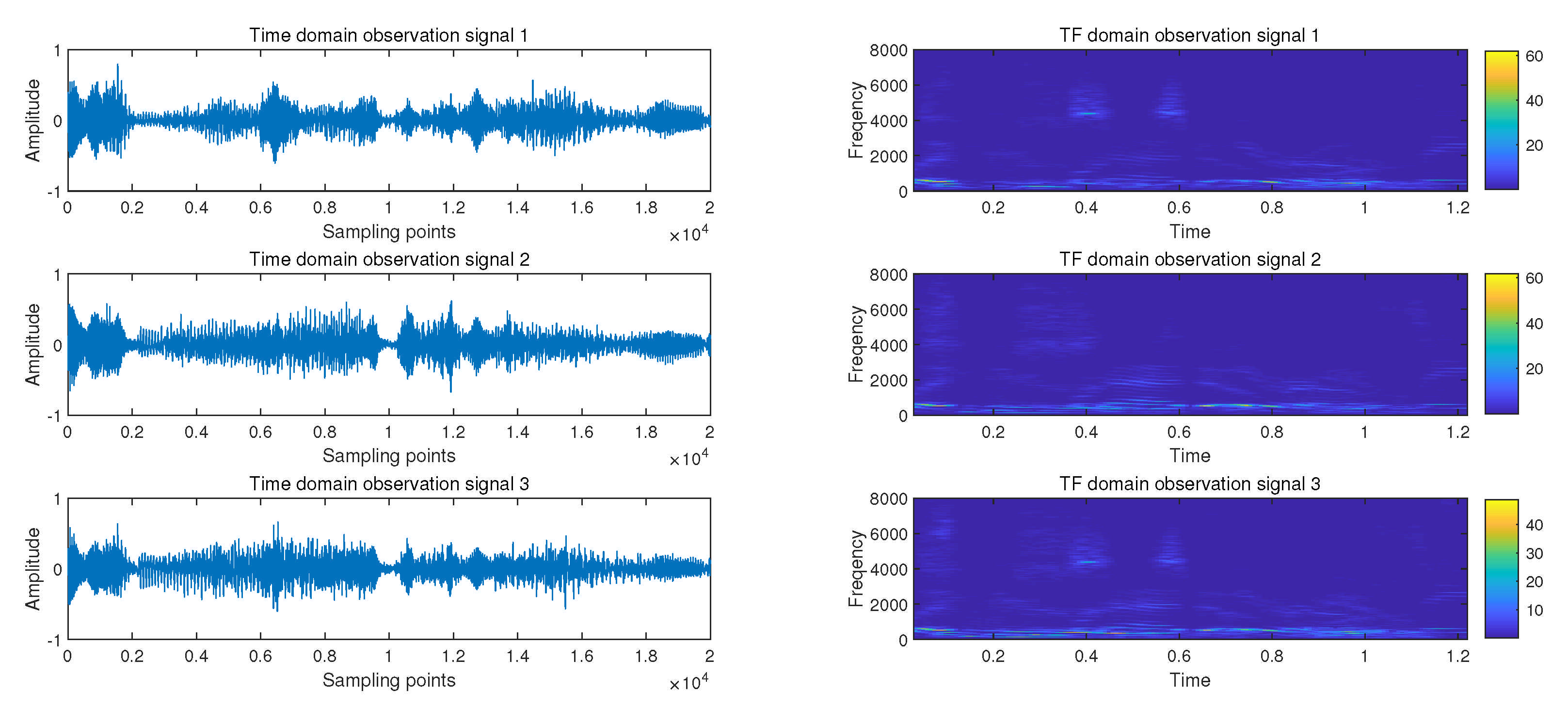
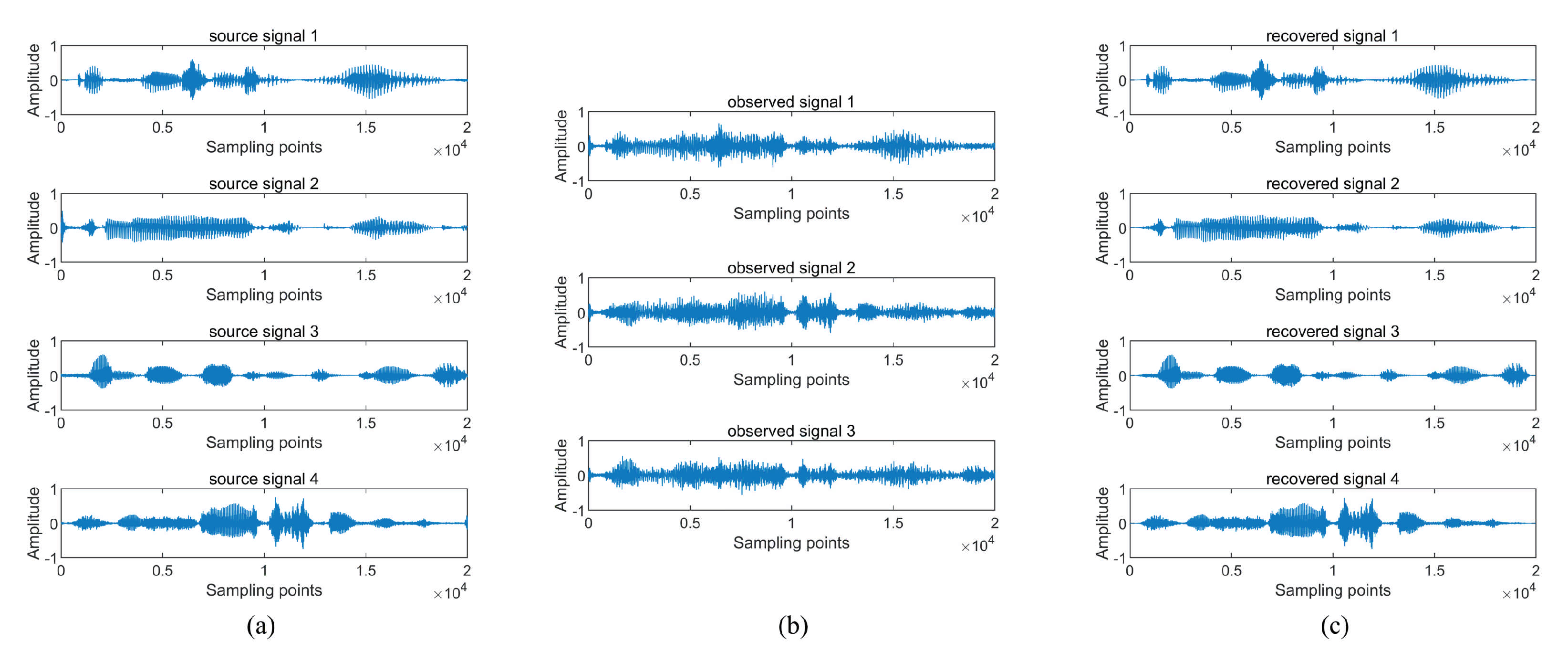
4.2.1. Experiment 1 A Complete Blind Source Separation Experiment

In experiment 1, 20,000 sampling points were selected as the four speech source signals, which were mixed to form three observed signals. The mixing matrix $\mathbf{A}$ is given as follows:

$$\mathbf{A}=\left[\begin{array}{cccc}\hfill 0.8005& \hfill 0.6587& \hfill -0.2456& \hfill -0.3480\\ \hfill 0.1291& \hfill -0.6002& \hfill -0.6028& \hfill 0.7974\\ \hfill 0.5853& \hfill 0.4538& \hfill 0.7591& \hfill 0.4930\end{array}\right]$$

(34)

Figure 4 shows the time domain waveform of mixed signal.

Table 1. Experiment 1 parameter settings.

Parameter	${\Delta }{\mathit{t}}_0$	${\Delta }{\mathit{f}}_0$	$\mathit{\phi }$	$\mathit{\lambda }$	$\mathit{\alpha }$	$\mathit{\mu }$
Value	3	3	0.99	0.2	0.1	0.99

shows the parameter settings for Experiment 1.

The scatter diagram of the observed signals in the time domain is shown in Figure 5a. As the signal does not meet the sparsity assumption in the time domain, the linear clustering characteristic described in Equation (3) does not appear. After the signal sparsity is enhanced by STFT, the TF domain scatter diagram of the observed signal is shown in Figure 5b and four clustering lines can be observed clearly. The scatter diagram of the remaining points after SSP screen is shown in Figure 5c. It can be seen that the outlier and noise points are effectively removed, and the line is clearer, which is beneficial to the accurate estimation of the mixing matrix.

Take the normalized SSPs as the input to the OPTICS algorithm. Taking the processing order of data points as the horizontal axis and the reachability-distance as the vertical axis, the algorithm decision diagram can be obtained as shown in Figure 6a. It can be seen that there are four obvious valleys in the figure, and the reachability-distance of data points in the valleys is close to 0, indicating that the SSPs form four tight clusters, and the cluster distribution is shown in Figure 6b. Set the denoising threshold $\rho$, represented by the red line in Figure 6a. The points with reachability-distance which are greater than $\rho$ are regarded as noise points and removed. The normalized scatter diagram after denoising is shown in Figure 6c, indicating that the points in the cluster are closely distributed. Using the improved potential function method to estimate the cluster center for the points in each cluster, the estimated mixing matrix can be obtained as follows:

$$\widehat{\mathbf{A}}=\left[\begin{array}{cccc}\hfill 0.8021& \hfill 0.6603& \hfill -0.2371& \hfill -0.3471\\ \hfill 0.1205& \hfill -0.5983& \hfill -0.6009& \hfill 0.7996\\ \hfill 0.5848& \hfill 0.4539& \hfill 0.7633& \hfill 0.4899\end{array}\right]$$

(35)

The improved subspace projection method is adopted to recover the source signal. The comparison between the source signals and the recovered signals is shown in Figure 7.

In this experiment, the NMSE estimated by the mixed matrix is −42.7103dB, and the SIRs of the four recovered signals are 34.4644dB, 20.3956dB, 17.0444dB, and 37.6604dB, respectively, with an average SIR of 27.3912dB. It can be seen that the algorithm can recover the source signal accurately.

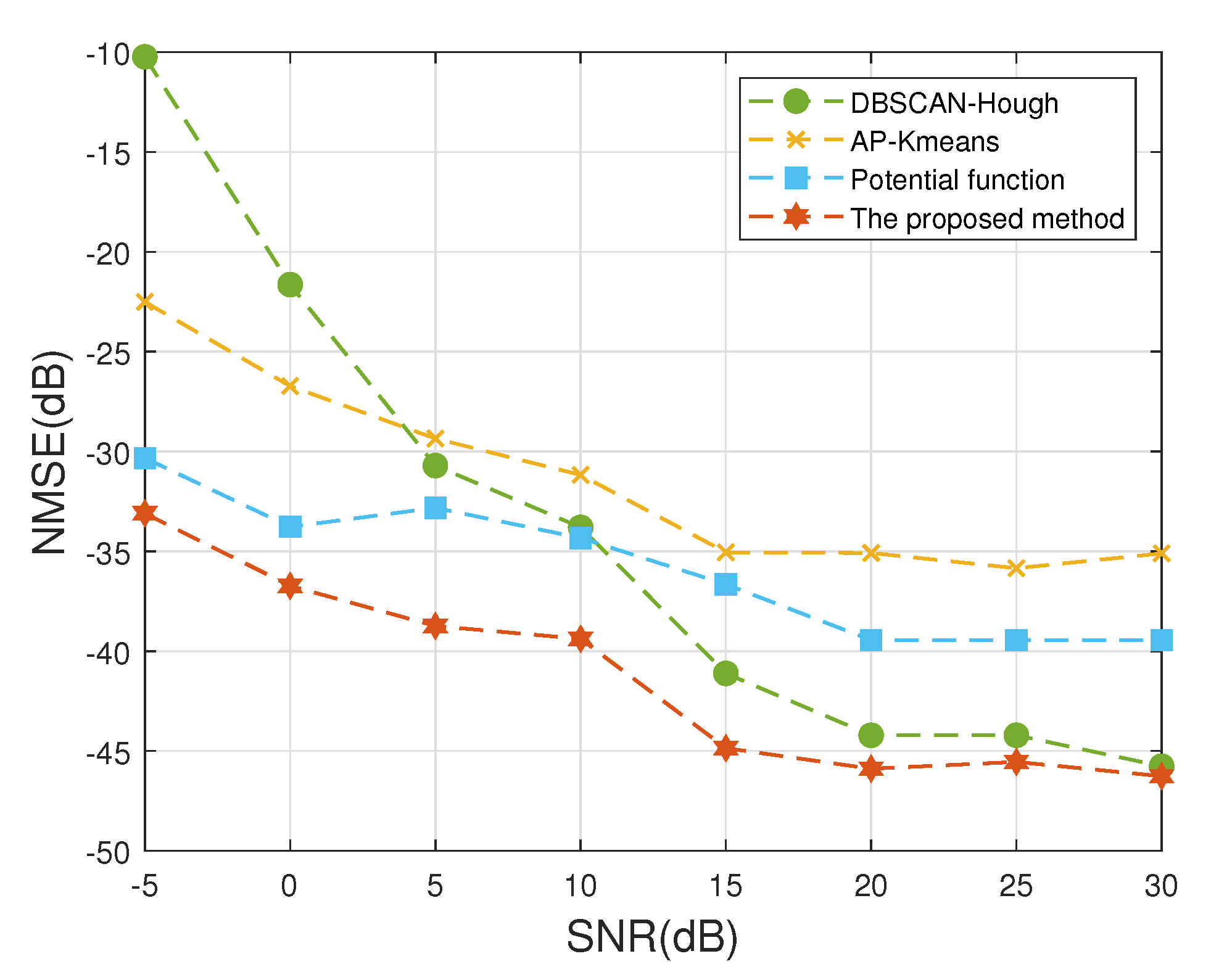
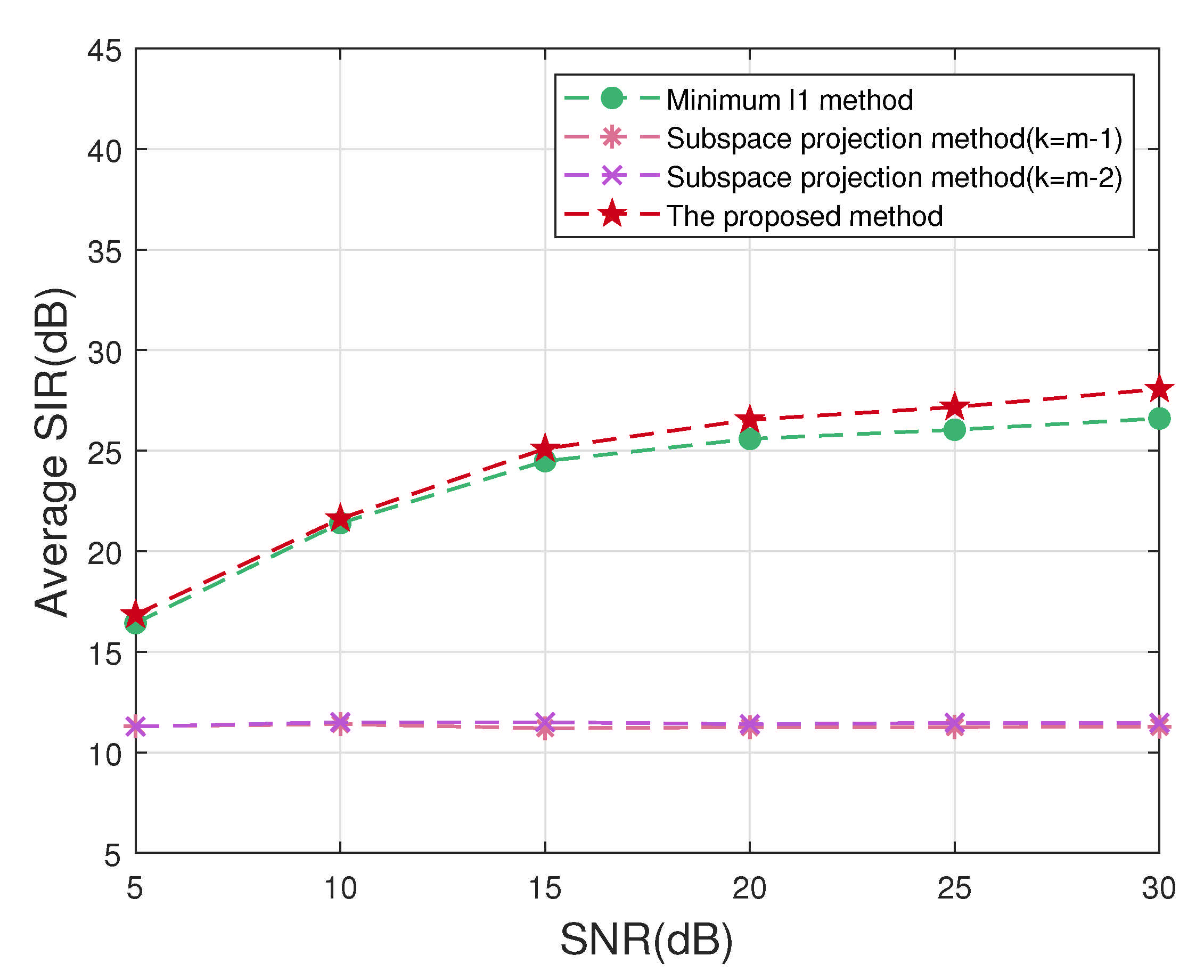
4.2.2. Experiment 2 Mixing Matrix Estimation Error

In the second experiment, in order to verify the accuracy of the proposed mixing matrix estimation method, we selected four speech signals and compared the accuracy of the proposed mixing matrix estimation method with DBSCAN-Hough [24], AP-Kmeans [25], and potential function method [23]. To compare the robustness of the method when dealing with noise, Gaussian white noise is added to the mixed signal. As the potential function method can only be applied to two-dimensional observed signals, the mixing matrix is selected as follows:

$$\mathbf{A}=\left[\begin{array}{cccc}\hfill 0.9872& \hfill 0.7392& \hfill 0.3773& \hfill -0.3999\\ \hfill 0.1592& \hfill 0.6735& \hfill 0.9261& \hfill 0.9165\end{array}\right]$$

(36)

In DBSCAN-Hough, $\beta =180$. In potential function method, $\lambda =5$, $h=0.2$, $K=90$. The results of the four algorithms are compared as shown in Figure 8.

DBSCAN-Hough and AP-Kmeans have a similar process with the mixing matrix estimation algorithm proposed in this paper. They use DBSCAN and AP clustering algorithms to classify the original data, respectively, and then use Hough transform and K-means to determine the cluster center within the cluster. According to the experimental data in Figure 8, when the SNR is high, both DBSCAN-Hough and the algorithm in this paper can obtain high accuracy, but the accuracy of AP-Kmeans and potential function method cannot be further improved. When the SNR is low, DBSCAN-Hough has a large error, mainly because DBSCAN is difficult to classify the data accurately at this time, and AP clustering is also difficult to classify the data accurately due to the influence of noise. The two methods above have a strong dependence on parameters. The proposed algorithm can also achieve better results at low SNR because the OPTICS algorithm reflects the density structure between the data and does not depend on the input parameters. According to the decision graph, the distribution of clusters can be determined intuitively and the noise points that affect the clustering effect can be removed. In addition, the improved potential function method can not only determine the cluster center accurately, but is also more practical than the traditional potential function method, which can be applied to the situation where the observed signal is greater than 2.

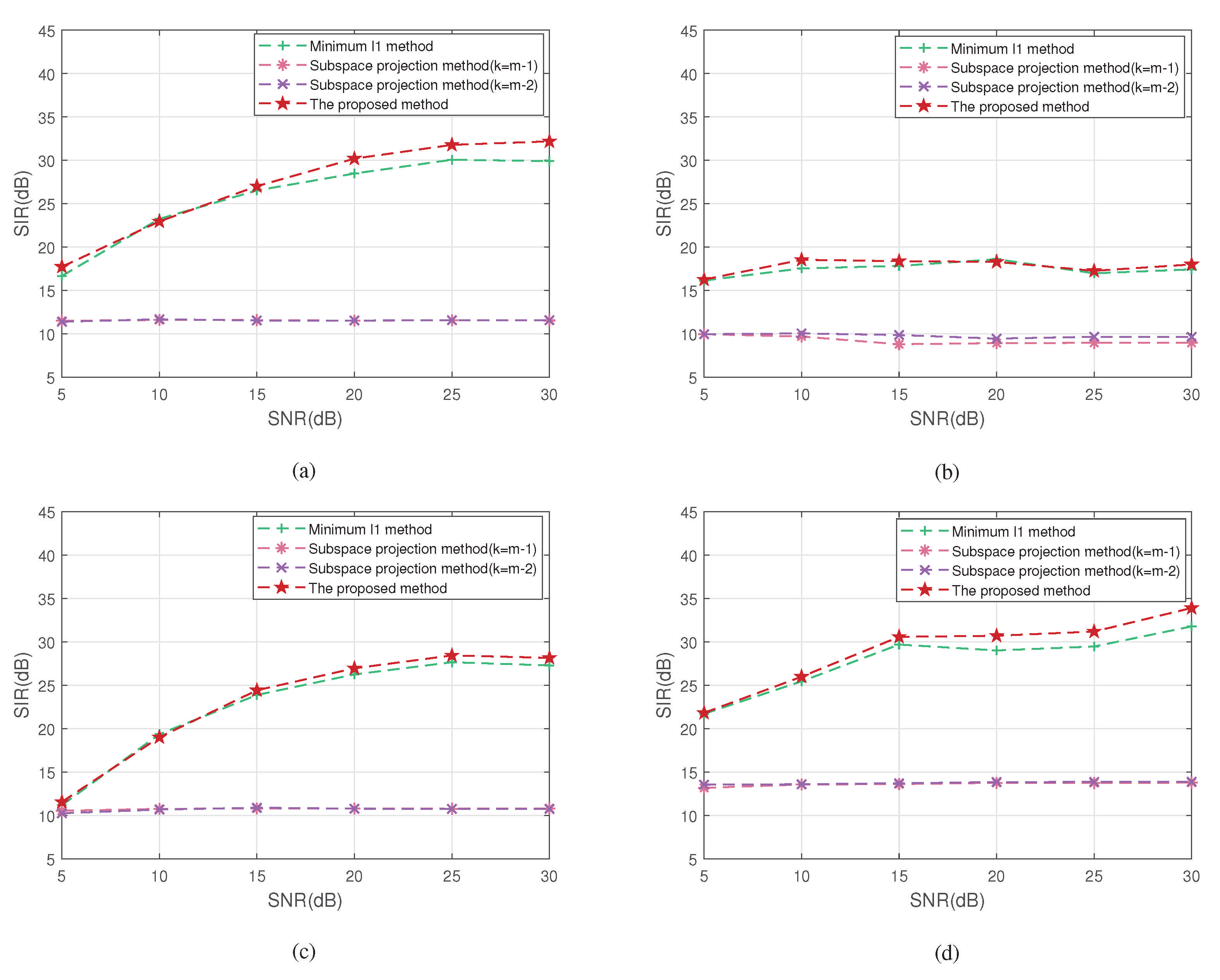
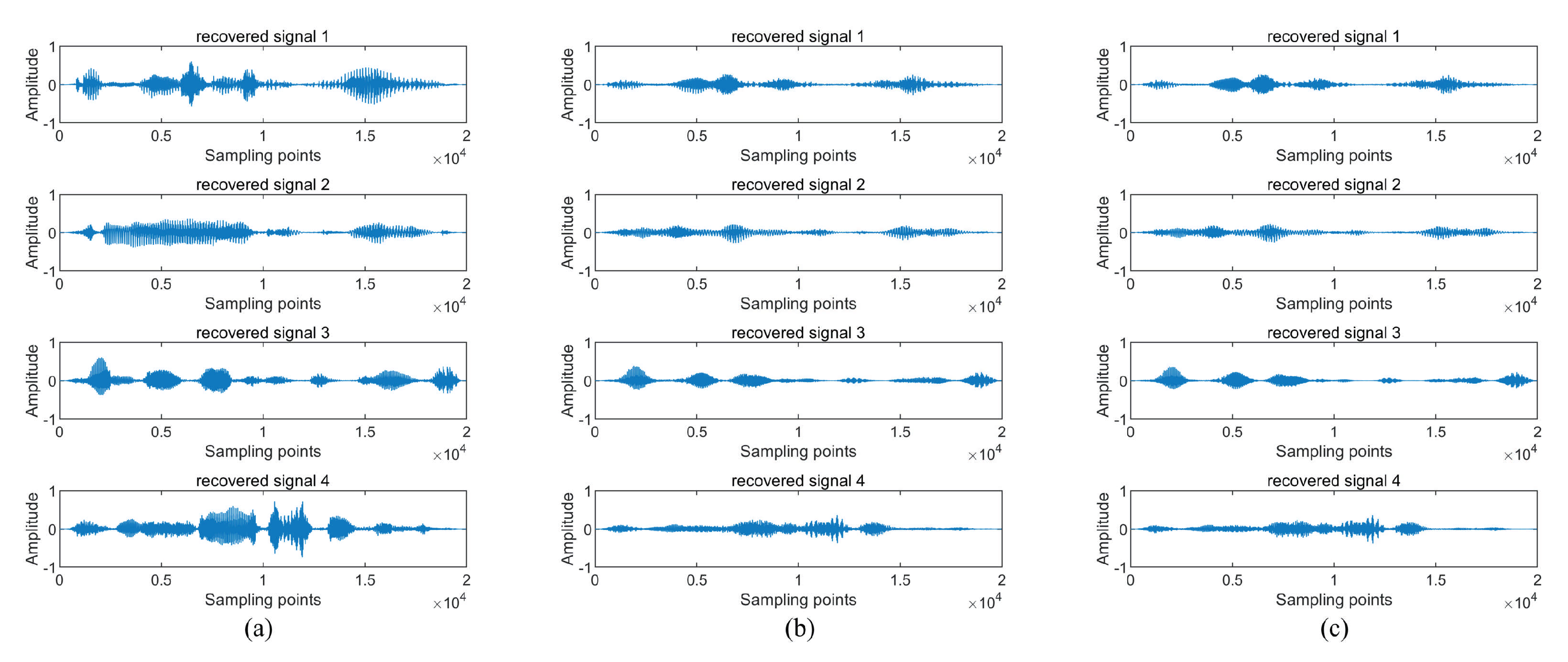
4.2.3. Experiment 3 Compares the Accuracy of Source Signal Recovery

In experiment 3, in order to verify the effectiveness and accuracy of the improved source signal recovery algorithm based on subspace projection, the proposed method was compared with the minimum ${\ell }_1$-norm method and the original subspace projection method. k represents the number of active source signals at any TF point in the original subspace projection method. Four segments of speech signals are mixed to get three mixed signals, which are separated in TF domain and restored to the time-domain signal by Inverse STFT. The recovery performance of the source signals is evaluated by the SIR. Without considering the noise, the source signal recovery effect of each method is shown in Figure 9 and Figure 10.

As can be seen above, compared with the original subspace projection method, the improved subspace projection method has better effect, and the time domain waveform is closer to the original signal. However, the results are similar to the minimum ${\ell }_1$-norm method. In the original subspace projection method, the recovery effect of $k=m-1$ and $k=m-2$ is similar, so the SIR of the recovered signal is quantitatively analyzed in

Table 2. SIR comparison of signal recovery using different methods.

Algorithm	The SIR of the Recovered Signal
	${\widehat{\mathit{s}}}_1$	${\widehat{\mathit{s}}}_2$	${\widehat{\mathit{s}}}_3$	${\widehat{\mathit{s}}}_4$	Average
Minimum ${\ell }_1$-norm method	30.6500	17.4698	28.5059	30.6469	26.8182
Original subspace projection method ($k=m-1$)	11.6024	8.9246	10.8156	13.7702	11.2782
Original subspace projection method ($k=m-2$)	11.5598	9.6417	10.7634	13.8636	11.4571
The proposed method	32.6860	17.7190	28.9573	33.3265	28.1722

.

The performance of the proposed method is compared with other methods when different levels of noise are added to the mixed signal. Figure 11 shows the SIR of the four recovered signals, and Figure 12 shows the average SIR. In order to eliminate the influence of the estimation error of the mixing matrix on the experimental results and guarantee the persuasiveness of the results, the actual mixing matrix is given as a known condition. In this experiment, set parameters $\mu =0.99$.

According to the results in Figure 11 and Figure 12, the original subspace projection method, when $k=m-1$ and $k=m-2$, has similar and poor signal recovery effects under different SNR conditions. The proposed method not only increases the upper limit of active sources at each TF point from $m-1$ to m, but also determines the number of active sources according to the projection value of each point in space, which makes the algorithm more accurate. The performance of the proposed algorithm is better than the other two methods.

5. Conclusions

In this paper, a novel method for solving the UBSS of linear instantaneous mixing signals is proposed. First, in order to obtain better sparsity, the signal is transformed from the time domain to the TF domain, and the SSPs are screened using the PCA method, which is based on the statistical features of TF points. Then, the density-based OPTICS clustering method is introduced to determine the data cluster distribution and the number of source signals from the decision graph visually, which facilitates further elimination of outliers. The improved potential function is used to determine the column vectors of the mixing matrix. Finally, the source signal recovery step combines the minimum ${\ell }_1$-norm method and subspace projection method that determine the number of source signals as a prerequisite. Simulation results show that the proposed method can realize its functions effectively, and perform better than other methods when dealing with different levels of noise. This method is more widely applicable.

References

1. Mogami, S.; Takamune, N.; Kitamura, D.; Saruwatari, H.; Takahashi, Y.; Kondo, K.; Ono, N. Independent Low-Rank Matrix Analysis Based on Time-Variant Sub-Gaussian Source Model for Determined Blind Source Separation. IEEE Trans. Audio Speech Lang. Process. 2020, 28, 503–518. [Google Scholar] [CrossRef]
2. Smith, S.; Pischella, M.; Terré, M. A Moment-Based Estimation Strategy for Underdetermined Single-Sensor Blind Source Separation. IEEE Signal Process. Lett. 2019, 26, 788–792. [Google Scholar] [CrossRef]
3. Batalheiro, P.B.; Petraglia, M.R.; Haddad, D.B. New efficient subband structures for blind source separation. Signal Process. 2021, 182, 107957. [Google Scholar] [CrossRef]
4. Xie, Y.; Xie, K.; Yang, J.; Xie, S. Underdetermined Blind Source Separation Combining Tensor Decomposition and Nonnegative Matrix Factorization. Symmetry 2018, 10, 521. [Google Scholar] [CrossRef] [Green Version]
5. Feng, F.; Kowalski, M. Underdetermined Reverberant Blind Source Separation: Sparse Approaches for Multiplicative and Convolutive Narrowband Approximation. IEEE Trans. Audio Speech Lang. Process. 2019, 27, 442–456. [Google Scholar] [CrossRef]
6. Zou, L.; Chen, X.; Dang, G.; Guo, Y.; Wang, Z.J. Removing Muscle Artifacts From EEG Data via Underdetermined Joint Blind Source Separation: A Simulation Study. IEEE Trans. Circuits Syst. II Exp. Briefs 2020, 67, 187–191. [Google Scholar] [CrossRef]
7. Niknazar, H.; Nasrabadi, A.M.; Shamsollahi, M.B. A new blind source separation approach based on dynamical similarity and its application on epileptic seizure prediction. Signal Process. 2021, 183, 108045. [Google Scholar] [CrossRef]
8. Guo, Q.; Li, C.; Ruan, G. Mixing Matrix Estimation of Underdetermined Blind Source Separation Based on Data Field and Improved FCM Clustering. Symmetry 2018, 10, 21. [Google Scholar] [CrossRef] [Green Version]
9. Gu, Z.; Fan, T.; Lv, Q.; Chen, J.; Ye, D.; Huangfu, J.; Sun, Y.; Zhu, W.; Li, C.; Ran, L. Remote Blind Motion Separation Using a Single-Tone SIMO Doppler Radar Sensor. IEEE Trans. Geosci. Remote Sens. 2019, 57, 462–472. [Google Scholar] [CrossRef]
10. Liu, Z.; Wang, L.; Feng, Y.; Qian, Z.; Xu, X.; Chen, X. A recognition method for time-frequency overlapped waveform-agile radar signals based on matrix transformation and multi-scale center point detection. Appl. Acoust. 2021, 175, 107855. [Google Scholar] [CrossRef]
11. Li, G.; Tang, G.; Wang, H.; Wang, Y. Blind source separation of composite bearing vibration signals with low-rank and sparse decomposition. Measurement 2019, 145, 323–334. [Google Scholar] [CrossRef]
12. Lu, J.; Cheng, W.; He, D.; Zi, Y. A novel underdetermined blind source separation method with noise and unknown source number. J. Sound Vib. 2019, 457, 67–91. [Google Scholar] [CrossRef]
13. Sen He, X.; He, F. Underdetermined mixing matrix estimation based on artificial bee colony optimization and single-source-point detection. Multimed. Tools Appl. 2020, 79, 13061–13087. [Google Scholar]
14. Underdetermined Blind Source Separation for linear instantaneous mixing system in the non-cooperative wireless communication. Phys. Commun. 2021, 45, 101255. [CrossRef]
15. Emura, S.; Sawada, H.; Araki, S.; Harada, N. Multi-Delay Sparse Approach to Residual Crosstalk Reduction for Blind Source Separation. IEEE Signal Process. Lett. 2020, 27, 1630–1634. [Google Scholar] [CrossRef]
16. Xiao, Y.; Lu, W.; Yan, Q.; Zhang, H. Blind separation of coherent multipath signals with impulsive interference and Gaussian noise in time-frequency domain. Signal Process. 2021, 178, 107750. [Google Scholar] [CrossRef]
17. Zou, L.; Chen, X.; Wang, Z.J. Underdetermined Joint Blind Source Separation for Two Datasets Based on Tensor Decomposition. IEEE Signal Process. Lett. 2016, 23, 673–677. [Google Scholar] [CrossRef]
18. Jourjine, A.; Rickard, S.; Yilmaz, O. Blind separation of disjoint orthogonal signals: Demixing N sources from 2 mixtures. In Proceedings of the 2000 IEEE International Conference on Acoustics, Speech, and Signal, Istanbul, Turkey, 5–9 June 2000; Volume 5, pp. 2985–2988. [Google Scholar]
19. Frédéric Abrard, Y.D. A time–frequency blind signal separation method applicable to underdetermined mixtures of dependent sources. Signal Process. 2005, 85, 1389–1403. [Google Scholar] [CrossRef]
20. Reju, V.; Koh, S.N.; Soon, I.Y. An algorithm for mixing matrix estimation in instantaneous blind source separation. Signal Process. 2009, 89, 1762–1773. [Google Scholar] [CrossRef]
21. Zhen, L.; Peng, D.; Yi, Z.; Xiang, Y.; Chen, P. Underdetermined Blind Source Separation Using Sparse Coding. IEEE Trans. Neural Netw. Learn. Syst. 2017, 28, 3102–3108. [Google Scholar] [CrossRef] [PubMed]
22. Zhen, L.; Peng, D.; Zhang, H.; Sang, Y.; Zhang, L. Underdetermined mixing matrix estimation by exploiting sparsity of sources. Measurement 2020, 152, 107268. [Google Scholar] [CrossRef]
23. Bofill, P.; Zibulevsky, M. Underdetermined blind source separation using sparse representations. Signal Process. 2001, 81, 2353–2362. [Google Scholar] [CrossRef] [Green Version]
24. Sun, J.; Li, Y.; Wen, J.; Yan, S. Novel mixing matrix estimation approach in underdetermined blind source separation. Neurocomputing 2016, 173, 623–632. [Google Scholar] [CrossRef]
25. Sen He, X.; He, F.; Hua Cai, W. Underdetermined BSS Based on K-means and AP Clustering. Circuits Syst. Signal Process. 2016, 35, 2881–2913. [Google Scholar]
26. Sen He, X.; He, F.; Xu, L. Underdetermined mixing matrix estimation based on joint density-based clustering algorithms. Multimed. Tools Appl. 2021, 80, 8281–8308. [Google Scholar]
27. Yang, J.; Guo, Y.; Yang, Z.; Xie, S. Under-Determined Convolutive Blind Source Separation Combining Density-Based Clustering and Sparse Reconstruction in Time-Frequency Domain. IEEE Trans. Circuits Syst. I Reg. Pap. 2019, 66, 3015–3027. [Google Scholar] [CrossRef]
28. Mohimani, H.; Babaie-Zadeh, M.; Jutten, C. A Fast Approach for Overcomplete Sparse Decomposition Based on Smoothed 0 Norm. IEEE Trans. Signal Process. 2009, 57, 289–301. [Google Scholar] [CrossRef] [Green Version]
29. Guoqing, R.; Qiang, G.; Gao, J. Novel underdetermined blind source separation algorithm based on compressed sensing and K-SVD. Trans. Emerg. Telecommun. Tech. 2017, 29, e3427. [Google Scholar]
30. Zhang, C.; Hao, D.; Hou, C.; Yin, X. A New Approach for Sparse Signal Recovery in Compressed Sensing Based on Minimizing Composite Trigonometric Function. IEEE Access 2018, 6, 44894–44904. [Google Scholar] [CrossRef]
31. Mirzaei, S.; Van Hamme, H.; Norouzi, Y. Blind audio source counting and separation of anechoic mixtures using the multichannel complex NMF framework. Signal Process. 2015, 115, 27–37. [Google Scholar] [CrossRef] [Green Version]
32. Nathwani, K.; Hegde, R.M. Joint source separation and dereverberation using constrained spectral divergence optimization. Signal Process. 2015, 106, 266–281. [Google Scholar] [CrossRef]
33. Aissa-El-Bey, A.; Linh-Trung, N.; Abed-Meraim, K.; Belouchrani, A.; Grenier, Y. Underdetermined Blind Separation of Nondisjoint Sources in the Time-Frequency Domain. IEEE Trans. Signal Process. 2007, 55, 897–907. [Google Scholar] [CrossRef] [Green Version]
34. Ankerst, M.; Breunig, M.M.; Kriegel, H.P.; Sander, J. OPTICS: Ordering Points to Identify the Clustering Structure. In Proceedings of the ACM SIGMOD International Conference on Management of Data, Philadelphia, PA, USA, 1–3 June 1999; pp. 2985–2988. [Google Scholar]
Figure 1. Block diagram of the proposed method.
Symmetry 13 01677 g001
Figure 2. OPTICS processing flow chart.
Symmetry 13 01677 g002
Figure 3. OPTICS algorithm decision diagram.
Symmetry 13 01677 g003
Figure 4. Time domain waveform of mixed signal.
Symmetry 13 01677 g004
Figure 5. (a) Time domain scatter plot of the observed signals. (b) TF domain scatter plot of the observed signals. (c) TF domain scatter plot after SSP screening.
Symmetry 13 01677 g005
Figure 6. (a) Decision diagram of OPTICS algorithm. (b) Normalized scatter diagram before noise removal. (c) Normalized scatter diagram after noise removal.
Symmetry 13 01677 g006
Figure 7. Comparison of source signal and recovery signal.
Symmetry 13 01677 g007
Figure 8. Comparison of estimation accuracy of mixing matrix.
Symmetry 13 01677 g008
Figure 9. Comparison of time domain recovery signals with different methods. (a) Source signals (b) mixed signals. (c) The signals recovered by proposed method.
Symmetry 13 01677 g009
Figure 10. Comparison of time domain recovery signals with different methods. (a) The signals recovered by the minimum 1 -norm method. (b) The signals recovered by the original subspace projection ( k = m 1 ). (c) The signals recovered by the original subspace projection ( k = m 2 ).
Symmetry 13 01677 g010
Figure 11. Signal recovery performance of different methods: panels (ad) correspond to s ^ 1 , s ^ 2 , s ^ 3 , and s ^ 4 , respectively.
Symmetry 13 01677 g011
Figure 12. Comparison of average SIR of signals recovered by different methods.
Symmetry 13 01677 g012