Majority Decision Aggregation with Binarized Data in Wireless Sensor Networks

Abstract

Wireless sensor networks (WSNs) are the cornerstone of the current Internet of Things era. They have limited resources and features, a smaller packet size than other types of networks, and dynamic multi-hop transmission. WSNs can monitor a particular area of interest and are used in many different applications. For example, during the COVID-19 pandemic, WSNs have been used to measure social distancing/contact tracing among people. However, the major challenge faced by WSN protocols is limited battery energy. Therefore, the whole WSN area is divided into odd clusters using k-means++ clustering to make a majority rule decision to reduce the amount of additional data sent to the base station (or sink) and achieve node energy-saving efficiency. This study proposes an energy-efficient binarized data aggregation (EEBDA) scheme, by which, through a threshold value, the collected sensing data are asserted with binary values. Subsequently, the corresponding cluster head (CH), according to the Hamming weight and the final majority decision, is calculated and sent to the base station (BS). The EEBDA is based on each cluster and divides the entire WSN area into four quadrants. All CHs construct a data-relay transmission link in the same quadrant; the binary value is transferred from the CHs to the sink. The EEBDA adopts a CH rotation scheme to aggregate the data based on the majority results in the cluster. The simulation results demonstrate that the EEBDA can reduce redundant data transmissions, average the energy consumption of nodes in the cluster, and obtain a better network lifetime when compared to the LEACH, LEACH-C, and DEEC algorithms.

1. Introduction

In recent years, wireless sensor networks (WSNs) have emerged as a topic of interest to most scholars because of the increasingly mature and advanced technology of micro-electro-mechanical systems (MEMS) and communication batteries, as well as improved communication technology and related application software [1,2]. The advantage of WSNs is their low implementation cost; there is no fixed infrastructure, and their deployment is arbitrary. Hundreds to thousands of sensor nodes are densely and arbitrarily deployed to sense areas of interest. Therefore, WSNs play an essential role in tracking and surveillance operations, such as habitat monitoring, weather forecasting, high accuracy agriculture, natural disaster prevention, border surveillance, smart cities, and home automation. They operate in an environment that does not require attended assistance with sensing, computation, and communication capabilities. Each sensor node can communicate among nodes and sends the gathered information using a multiple-hop relay. The base station (BS) is generally fixed and arbitrarily deployed far from these sensors. Because the communication distance between the sensor nodes and the BS is considerable, the energy will be exhausted quickly. Thus, the main factor influencing the total energy consumption is data transfer over a distance between nodes. Furthermore, because of nodes’ dense deployment for optimal data resolution, the consequences of sensor node redundancy are data highly correlated, producing unnecessary data transmissions from nodes owing to overlapping sensing areas. The degree of data correlation causes redundant data and the additional energy consumption of the nodes [3,4].

The sensor nodes use the sensed original sensor signals to assert a binary value of one or zero by defining a threshold, thereby transferring binary values to the cluster head (CH) in the same cluster. Subsequently, the CH performs data aggregation and the majority decision through the Hamming weight (HW). Thus, in addition to reducing the redundant transmission of data, the reporting nodes can also save energy and extend the lifetime of the entire network [5]. Therefore, this study includes the following proposals:

• The calculation method for defining the k value of k-means++ to ensure that the distance between nodes in the cluster is less than the threshold value between transmission and reception in the first-order radio model and provides further energy-saving efficiency and extends the overall network lifetime.
• The k value is defined as an odd number, which means that there will be an odd cluster and cluster head, and the purpose is to aggregate the binarized data to a BS to achieve a majority decision afterward.
• Once the nodes are deployed, the sensing nodes must operate for months or years without any additional power supply. Notably, the communication between nodes often consumes more energy than the computation. If the original sensing data are directly transmitted to the sink, it will consume much more energy. WSNs are often used in alarm applications. Moreover, we have assumed that a critical threshold value is the warning level and is asserted/deasserted a binary. Only binary values are transmitted, which conserves energy at the node and extends the network’s lifetime.
• The BS is fixedly deployed in the center of the sensing area. The sensing area consumes the center of the entire WSN and is used as the origin to further divide it into four quadrants. A data transmission chain is constructed in each quadrant. The chain starts from the CH farthest from the BS, and ends at the CH nearest to the BS. In each round, the CH transmits the majority binary value to the next hop until it reaches the BS by the chain. This is a proven method of reducing CH energy consumption.

The remainder of this paper is organized as follows: Section 2 describes related research examining the energy consumption, energy efficiency, cluster head selection, and cluster formation in a WSN used, and applying the Hamming weight to count the number of non-zero bits to obtain the majority result. Section 3 discusses the working principle of our proposed EEBDA scheme in detail. In Section 4, the performance of the proposed EEBDA against other related protocols is evaluated. Section 5 discusses, evaluates, and compares the results with other protocols. Finally, we conclude the study and discuss future work in Section 6.

2. Related Works

Many routings, energy management, and data propagation protocols have been specifically developed for WSNs, where energy-efficient realization is an essential design issue. Akyildiz et al. [6] and Mohamed et al. [7] described randomly distributed sensor nodes. Each sensor node does not know its position relative to other sensor nodes; therefore, the WSN must have a self-organization protocol, a self-organization communication network between sensor nodes to transmit data. Because WSNs often operate in a severe, unsupervised environment, monitoring activities cannot be managed efficiently without manual involvement. In such surroundings, a large number of randomly deployed sensor nodes guarantee fine-grained surveillance. Furthermore, in the routing and data collection protocols, energy efficiency should be considered as a design priority in order to maximize the lifetime of the network. In WSNs, the practice of grouping nodes into clusters has been commonly applied. It combines routing and data collection protocols to achieve high energy efficiency and maximize the network lifetime. These hierarchical data collection protocols provide data fusion and aggregation through cluster-based groups of nodes. Consequently, they minimize the energy consumption of the nodes to sustain the long-term running of the WSNs [8,9].

2.1. Majority Rule and Hamming Weight

A majority rule is a decision-making rule that chooses alternatives with a majority of votes, that is, more than half of the votes. Decisions are an essential part of group activities, especially in densely deployed sensor networks where the energy consumption of node data transmission can be saved by producing final results through a majority decision. In addition, majority decisions can report that the final event indication is of interest without any other details of the event. Equation (1) denotes the results of majority decisions, where n is eligible voters who participate in an election [10,11].

$$M_{result}=\lceil \frac{n+1}{2}\rceil$$

(1)

For low-energy and fault-prone sensor nodes that are vulnerable, Biswas et al. [12] presented a true event-driven and fault-tolerant routing (TED-FTR) algorithm that sends a report to the BS through multiple hops. The ambiguity of the fault measurements is eliminated using the majority voting algorithm among neighbors to identify an actual event. If most neighbors experience identical but unusual results, the node considers it an event and sends a report to the BS. In [12], majority voting is performed to disambiguate the reporting event of neighbor nodes. The majority voting algorithm uses Equation (2), which is given below. Suppose $N_i$ has j number of neighbors, $N_i\left(1\right)$,$N_i\left(2\right)$,…$N_i\left(j\right)$, with binary decisions, $B{d}_i^p\left(1\right),B{d}_i^p\left(2\right),\dots B{d}_i^p\left(j\right),$as given in Equation (2).

$$Even{t}_i^p=\left\{\begin{array}{c}1 if \left|\left\{k|B{d}_i^p\left(k\right)=1\right\}\right|\ge \left|\left\{k|B{d}_i^p\left(k\right)=0\right\}\right|\\ 0 otherwise\end{array}\right.$$

(2)

where $\left|\left\{k|B{d}_i^p\left(k\right)=1\right\}\right|$ is the number of neighbor nodes, replied to with a binary decision (Bd). If the number of $\left|\left\{k|B{d}_i^p\left(k\right)=1\right\}\right|$ is greater than or equal to the number of $\left|\left\{k|B{d}_i^p\left(k\right)=0\right\}\right|$, that is, the majority of neighbors vote is a binary decision (Bd) 1, N_i sets $Even{t}_i^p=1$, otherwise 0 using Equation (2). TED-FTR does not exhibit better performance in scenarios where more nodes are faulty or there are failures because the nodes responsible for reporting event information can quickly consume their energy.

Irving S. Reed formulated a concept to the Hamming weight equivalent in a binary case in 1953 [13]. The Hamming weight of the binary vector $v\in {\left\{0, 1\right\}}^n$ is a number that ranges from 0 to n, which is defined as $W_H\left|v\right|={\displaystyle \sum }_{i=1}^n{v}_i=\left|\left\{v_i \in \left[n\right]: v_i=1\right\}\right|$. We can count the number of non-zero entries in vector V by the Hamming weight. The weight w of a code word is the number of 1s in the vector to determine whether one is the majority by the majority function. For example, the word 11,101,010 weighs five. Formally speaking, for n odd, the majority function is given by the $MA{J}_n\left(v_1,\dots ,v_n\right)=1$, if and only if $\left[v_1+v_2+\dots +v_n\right]\ge \lceil \frac{n}{2}\rceil$. In this study, we present the idea of majority decision making and its application to the majority voting of Hamming weights [14], which are asserted with a binary value of one or zero through a threshold value within the same cluster; that is, the number of non-zero bits in the binary sequence. Thus, according to the definition of the Hamming weight, the number of non-zeros in the given input binary sensing data is calculated to find the final majority result in the cluster.

2.2. Spatial Correlation Model for Sensor Networks

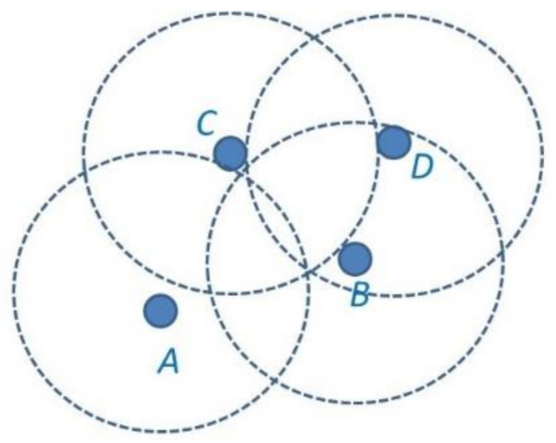
Because communication is the primary bottleneck in energy consumption of the node, rather than computation [15], the sensors are densely deployed to cause overlapping in the sensing area, which leads to redundancy in the sensing data, and a high correlation in the data, thus resulting in a large volume of communication. That is to say, spatial correlation also implies a high data correlation between the nodes. In this study, we intended to exploit the spatial and data correlation to limit the number of reporting nodes to achieve a minimum number of reporting nodes, while still maintaining data resolution. Thus, the motivation is to design a significant amount of energy efficiency aggregation mechanisms for energy-constrained WSNs by exploiting spatial and data correlation. Figure 1 illustrates the overlapping sensing area leading to data redundancy of some nodes.

Yin et al. [16] considered spatial clustering and principal component analysis (PCA) techniques in which sensors with a hardy temporal–spatial correlation are grouped into a cluster to facilitate further processing with novel efficient data compression schemes. To conserve energy and prolong the lifetime of WSNs, the authors designed an adaptive CH selection scheme that finds the CH dynamically and minimizes energy consumption. In addition, the CH applies PCA with an error constraint guarantee to compress and handle the data using a predefined compression algorithm. CH requires additional PCA and error-bound guarantees to compress the data that utilizes multiple computing resources. Therefore, it may not apply to most low-energy WSNs. Leandro A. Villas et al. [17] proposed a dynamic and scalable tree aware of spatial correlation (YEAST) algorithm. YEAST is a spatial correlation-aware dynamic and scalable routing structure for data gathering and aggregation in WSNs. The YEAST algorithm builds a routing tree using the shortest paths (in Euclidean distance), connecting all coordinator nodes and sink nodes while maximizing data aggregation and minimizing distances. Furthermore, YEAST does not build a routing tree by order of events. Thus, with YEAST, an event can be sensed more accurately, and the residual energy of the node can be saved from the sensing area, in contrast to the classical approach to data gathering. YEAST at during network formation and maintenance, nodes exchange control information, which control message results in more energy depletion. Therefore, YEAST is not feasible for large-scale WSNs with long-duration events because the calculated shortest paths require a large amount of computation and control messages to be exchanged, which quickly consumes the energy of the nodes. The data aggregation scheme does not consider reducing the number of data values transferred between the ordinary sensors and the CHs. Hence, it is one of the objectives of our study. Tayeh, G.B. et al. [18] proposed a spatial–temporal correlation-based approach for sampling and transmission rate adaptation (STCSTA) in cluster-based sensor networks. A data reduction mechanism exploits the spatial–temporal correlation among sensor data to deploy nodes and formulate a sampling strategy. Moreover, the authors designed a back-end algorithm to find the spatial and temporal correlation among the reported dataset and fill the non-sampled parts with predictions for reporting the data to the sink. Redundancy deployment, residual energy, and distance to the sink are desired to avoid void area creation because no void handling mechanism has been proposed. Sensor measurement faults were not considered, resulting in a transmission delay and adding to the data discovery process. Thus, it is necessary for a well-designed data transmission model that can reduce the amount of data transmission while guaranteeing the requirement of data reliability.

Data correlation is extensively used in data reduction techniques. For example, the sensing area of the sensor nodes could be optimized based on a coincident overlapping coverage area with its neighbors. This study avoided data redundancy by reducing the reporting of correlated data in an environment with high node coverage redundancy, considering that spatial correlation can lead to data collision. In addition, the excessive energy consumption of CH can be reduced by CH rotation.

2.3. First-Order Radio Model

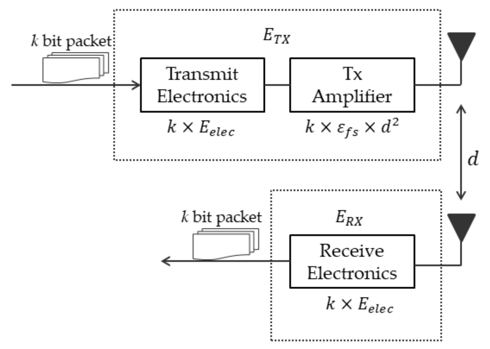
The first-order radio model is a widespread radio module used in WSN research. It is often used in the simulation analysis of sensor nodes. When data are transmitted via a wireless network, the distance is the main factor that affects the energy consumption of the sensor nodes. Based on our understanding, the wireless communication component of a sensor node is the critical component that consumes the most energy. We used the radio model shown in Figure 2 [19]. The first-order radio model evaluates the energy consumed when a sensor node transmits or receives at each cycle. The radio model has power control and can expend the minimum energy required to reach the intended recipients. For example, when a k-bit message is transmitted through a distance (d), the required energy can be expressed as shown in Equation (3), and the energy consumed at the reception is illustrated in Equation (4).

$$E_{TX}=E_{TX-elec}\times k+E_{TX-amp}\left(d^2\times k\right)=\left\{\begin{array}{c}k{E}_{elec}+k{\epsilon }_{fs}{d}^2, d<d_0\\ k{E}_{elec}+k{\epsilon }_{mp}{d}^4, d\ge d_0\end{array}\right.$$

(3)

$$E_{RX}=E_{RX-elec}\times k$$

(4)

where $E_{TX-elec}$ and $E_{RX}$ are the energy dissipated per bit of the transmitter and receiver, respectively. ${\epsilon }_{fs}$ and ${\epsilon }_{mp}$ depend on the transmitter amplifier model used, and d is the distance between the sender and receiver. In Equation (3), the distance d between nodes must be less than the threshold distance d₀, $k{\epsilon }_{fs}{d}^2$ according to the free space model; otherwise, ${\mathsf{\epsilon }}_{mp}{d}^4$ uses the multipath model. In this study, we assumed that the radio model dissipates $E_{elec}$= 50 nj/bit, ${\epsilon }_{fs}=10\mathrm{pJ}/\mathrm{bit}/{\mathrm{m}}^2$ and ${\epsilon }_{mp}=100\mathrm{pJ}/\mathrm{bit}/{\mathrm{m}}^2$, where $d_0=\sqrt{\left({\epsilon }_{fs}/{\epsilon }_{mp}\right)}\cong \sqrt{\frac{10}{0.0013}}\cong 87.705802$ denotes the threshold distance between two nodes.

2.4. Cluster-Based WSNs

In clustering, hierarchical schemes have a significant advantage in minimizing energy consumption. Clustering is one of the techniques in machine learning that involves grouping of data points. Given a set of data points and the conditions for classification, we used the clustering algorithm to classify each data point into a specific group. Thus, data points in the same group must contain similar attributes, while those in different groups must contain considerably different attributes. Clustering is an unsupervised learning method that is commonly used for statistical data analysis in many fields [20]. Owing to its many advantages, clustering is emerging as an attractive branch of routing technology in WSNs. Clustering is the process of dividing sensor nodes into groups based on specific characteristics. Typically, clusters are formed based on geographical location, residual energy, or distance from the BS. Each cluster selects a CH, which has more duties than cluster members. In cluster-based approaches, nodes are divided into different clusters based on their distance from each other, where a capable and plentiful energy sensor node is responsible for a cluster. In [19,21], the authors surveyed and discussed the design of cluster-based schemes, essential parameters for cluster formation, and classification of hierarchical clustering protocols. In addition, available cluster-based and grid-based techniques were appraised by regarding specific parameters to assist researchers evaluate suitable techniques.

Clustering and election of CHs for WSNs can be distributed or centralized. In a distributed mechanism, each sensor node broadcasts its location and energy level to its one-hop neighbors, and a node with a higher energy level and clustering concentration is elected as CH. In the centralized mechanism, after the BS advertises the request message, all nodes reply with their location and residual energy level to the BS, and the BS randomly selects a node as the CH to form a new cluster and broadcast itself to all the nodes. In a homogeneous sensor network, the CH is selected from the alive nodes. 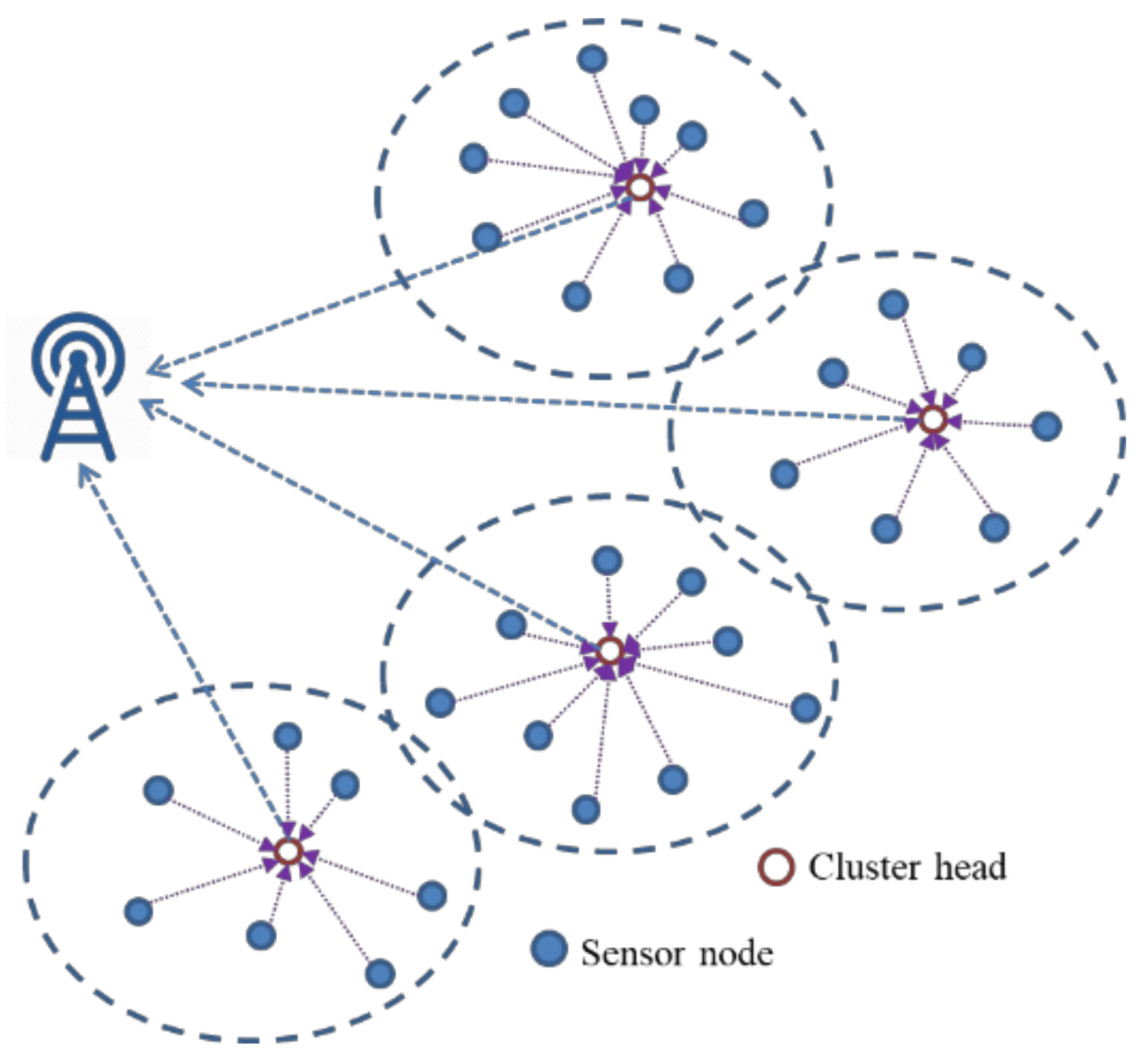CHs are responsible for transmitting sensing data from other nodes for data aggregation within the cluster and communication with the BS, thus saving general node energy [22]. Many scholars have proposed clustering-based routing protocol techniques to improve the energy efficiency of WSNs, as only a few CHs are allowed to contact the BS directly. The CHs are responsible for collecting data from their respective cluster members, processing it, and further communicating it to the BS. Quan Wang et al. [23], suggested that by organizing sensor nodes into clusters with the help of data aggregation/fusion mechanisms, energy-efficient use can be obtained as the total amount of data sent to the BS is significantly reduced. Moreover, intra-cluster communication minimizes the communication distance and energy dissipation of cluster members. Cluster routing protocols based on clustering algorithms have been proposed to manage the data communication in WSNs [24,25] (Figure 3).

2.4.1. K-means++ Clustering Algorithm

K-means clustering is a widely used clustering technology that attempts to minimize the average squared distance between data points in the same cluster. It was proposed in 1967 by MacQueen [26] and is sometimes called the Lloyd–Forgy algorithm. Its ease of implementation, computational efficiency, reduction in the complexity of the data, and low memory consumption have maintained the popularity of K-means clustering compared to other clustering techniques. However, the disadvantage is that the initial cluster centers are still selected arbitrarily, which may cause the concentration of all the initial cluster centers. In addition, K-means clustering is highly exponential in the k value, and it is difficult to determine the number of clusters (k) at the beginning of the algorithm, making it complex in practice.

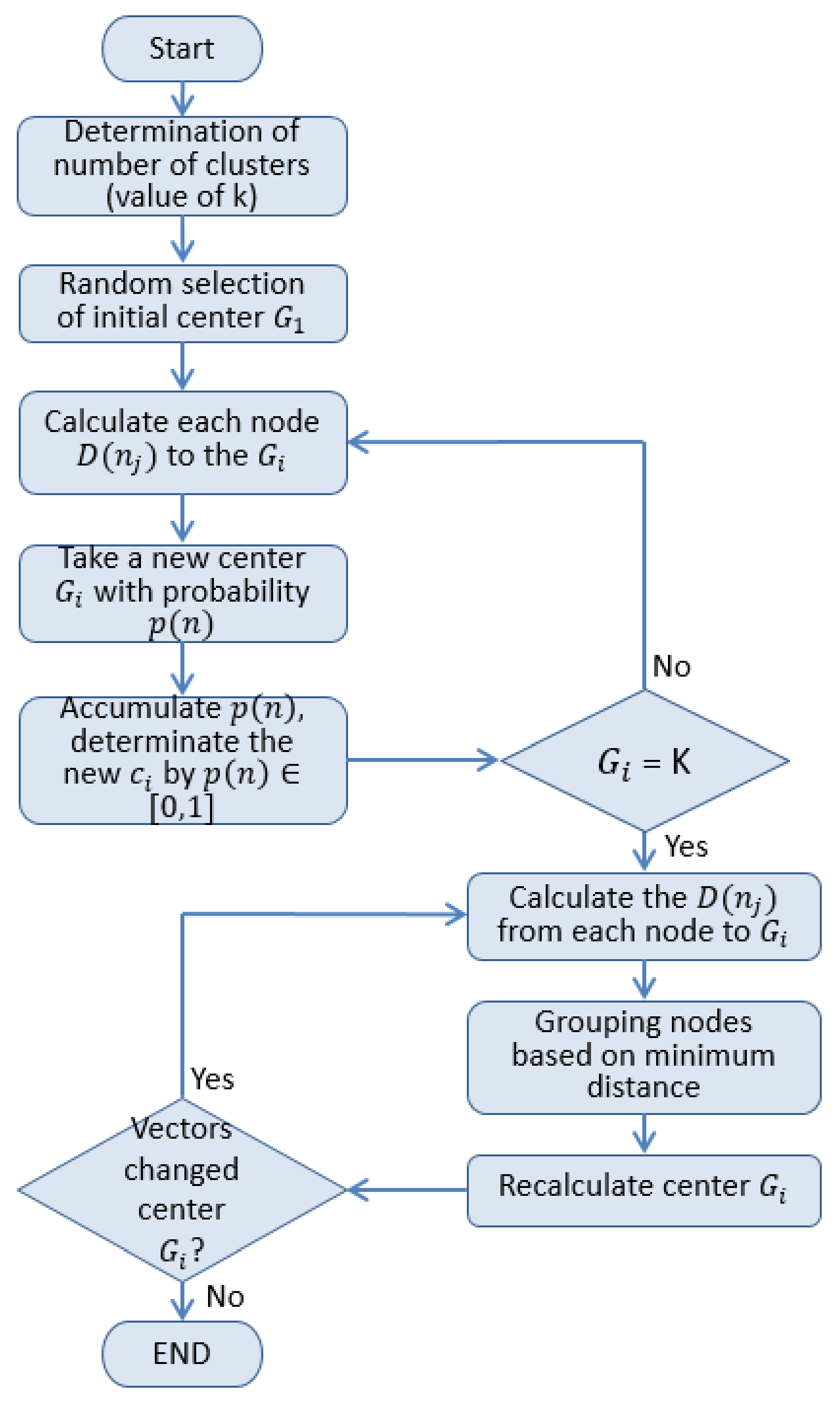
Vassilvitskii and Arthur [27] proposed a specific method to improve the problem of randomly selecting the initial cluster center. The k-means++ algorithm takes these data points as initial centers that are as distant from each other as possible. In particular, this method, which is called the k-means++, involves letting D(n) denote the shortest distance from a data point to the closest center that has already been chosen. K-means++ clustering improves the random selection of initial cluster centers and the possible over-concentration of cluster centers in K-means clustering. Figure 4 shows the flowchart of k-means++ clustering in our study, which was used to determine the number of k clusters based on the threshold distance of the first-order radio model over the entire sensing area. G_i is the ith clustering center for each $i\in \left\{1,\dots ,k\right\}$. Choosing the next center G_i+1 and selecting G_i with probability ($p\left(n\right)=\frac{D{\left(n^{\prime }\right)}^2}{\sum D{\left(n\right)}^2}$), the distance between two nodes was calculated using the Euclidean distance D(n). Therefore, we could use the k-means++ algorithm to divide the clusters evenly in the clustering phase.

2.4.2. Cluster-Based Routing Protocol for WSNs

Clustering is one of the most effective solutions to energy issues, which balances the energy consumption of the entire network by a cluster-based architecture to prolong the network lifetime. Sensor nodes are divided into different clusters based on their distance from each other, where a capable and plentiful energy sensor node is responsible for a CH. The CH collects data from the sensor member nodes and forwards them to the sink node. In cluster-based architectures, cluster formation and the selection of the cluster head node determine the network lifetime [21,28].

Low-energy adaptive clustering hierarchy (LEACH) [19] is one of the typical clustering-based routing protocols in WSNs. In LEACH, CHs are randomly selected based on a predefined percentage of CHs in the proposed network and the number of times that a node has been a CH thus far. Each non-CH node in the current round looks for the nearest CH to join as a member. CHs collect and aggregate data from their members. Finally, the CHs transmit the aggregated data directly to the sink nodes. As LEACH is a random selection of CHs, the number of CHs in each round is different. Every cluster also contains a different number of nodes in each round. Therefore, the energy consumption is not balanced in the overall network, in all the rounds. According to Equation (5), which is used to determine the threshold value T(n), every node in the network produces a randomly generated number (P) between 0 and 1, and if the number is less than the threshold value T(n), then the node is defined as a cluster head. The CH broadcasts an advertisement message to all other members in the cluster in the current round.

$$T\left(n\right)=\left\{\begin{array}{c}\frac{P}{1-P\left[r mod\left(\frac{1}{P}\right)\right]} if n\in G\\ 0 otherwise\end{array}\right.$$

(5)

where T(n) determines the threshold value of CH, r denotes the current round, P is the desired percentage of cluster heads, and G is the set of nodes that have not been CHs in the last 1/P rounds.

A centralized LEACH (LEACH-C) clustering algorithm with sensor networks was introduced in [29]. This algorithm improved the original LEACH algorithm. A BS selects a CH to improve the CH selection algorithm, whereas in the LEACH cluster, the cluster heads are selected randomly by the node itself. As with the LEACH protocol, LEACH-C has two phases: the setup phase and the steady-state phase. First, the BS selects the CH with the highest average energy, location, and energy level in the setup phase and uses it to aggregate the node data for transmission. After the BS selects the primary CH and associated clusters, the BS then broadcasts a message to all nodes, including the cluster head ID. If the cluster head ID matches its ID, the node is a CH; otherwise, it determines its time division multiple access (TDMA) slot for data transmission and, if it is not assigned to a TDMA slot, goes to sleep until it is time to transmit data. The steady-state phase of LEACH-C is similar to that of the LEACH protocol. Thus, the LEACH-C protocol improves the network lifetime as compared with the LEACH protocol. However, LEACH-C is unsuitable for large network areas, and isolated nodes cannot transmit their coordinates and residual energy to the BS. This results in severe data loss and degradation of network performance.

LEACH-Z (LEACH zones) and S-LEACH protocols [30,31] are both improved versions of LEACH. LEACH-Z protocol, divided into the cluster method is based on the larger clusters near the BS (i.e., a greater number of nodes). On the contrary, the smaller clusters are far away from BS. Thus, the smaller clusters prevent the election of CHs, thus reducing the data to be sent, by multiple hops and conserves energy. However, dividing the cluster size by the distance from the BS may still result in an energy hole or hot spot area. This may lead to non-collection of required data from all corners, which would ultimately affect the network performance. S-LEACH uses meta-data before receiving packets, an advantage of this feature, so that there are no identical or similar packets. This makes it possible to reduce the amount of redundant data transmission. However, S-LEACH encounters a challenge as it requires extra overhead to identify the meta-data, or data packet.

Li Qing et al. [32] studied a distributed energy-efficient clustering (DEEC) scheme for heterogeneous WSNs. In DEEC, considering the heterogeneity of the network, nodes cannot all consume the same amount of energy for data transmission. Therefore, a probability is used to select CH based on the ratio between the remaining energy of each node and the average energy of the network, and, accordingly, the energy of each node is used to adapt its rotation period. The nodes with high initial and residual energy will have more cluster heads than those with low energy. The authors demonstrated that simulation results showed that DEEC achieved a longer lifetime and more energy efficiency than the current necessary clustering protocols in heterogeneous environments, especially the stability period. However, this CH selection scheme may penalize the plentiful energy nodes because these nodes will be a CH consecutively, and they will die quicker than the others, especially when their residual energy depletes and comes within the range of the ordinary nodes.

It can be seen from the above literature that clustering can improve energy efficiency, and the CH is responsible for the data reporting within the cluster. However, the CH is still selected based on probability, and cluster size determination is also by probability, which may cause the CHs to be too centralized or scattered. Therefore, this study used residual energy, degree of data correlation, and binarization of data as the proposed CH selection and data aggregation parameters. As a result, it balances the load among clusters and reduces the energy consumption by further dividing the quadrants. Therefore, this study proposes an energy-efficient binarized data aggregation mechanism (EEBDA) with a spatial correlation among sensor nodes to avoid high correlation among data and reduce node redundancy data transmission.

2.4.3. Cluster Head Rotation in WSNs

In clustering, hierarchical techniques have significant advantages in minimizing energy consumption [33]. Therefore, to maximize the network lifetime, cluster head selection methods should be implemented appropriately. CH selection is a critical challenge to achieving energy efficiency and maximizing network lifetime. The authors considered the distance from the sensors to the BS for the optimal balance of energy consumption between nodes [34]. The main focus is on cluster formation and CH selection, taking into account the energy consumption and their effect on the overall network lifetime. In most techniques, the selection of CH considers several parameters, such as energy level, a node’s location, or the usage of a probabilistic approach, or it is performed through any random technique [19]. The reselection CH technique has a fast execution and convergence time, minimizes the number of exchanged messages, and reduces the number of CH rotations as much as possible. Therefore, CH selection with the highest residual energy nearest to the cluster center was the first choice in this study. 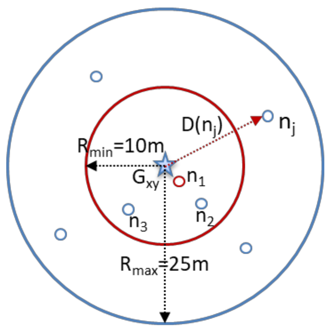Subsequently, CH rotation is evaluated by considering certain parameters to help us in rotating CH-appropriate opportunities, such as residual energy (Er) and minimum Euclidean distance from the group center. We chose the node near the group center because the CH is beneficial in balancing the transmission energy consumption within the cluster and reducing the communication distance between clusters. Figure 5 illustrates the scanning area of cluster head rotation, where G_xy is the group center, and D(n_j) is the Euclidean distance from the G_xy to node (n_j). The n₁ will be preferentially selected as the CH because it is closest to the group center.

3. The Proposed Approach (EEBDA)

In general, each node is designed with a limited battery power to operate in the WSNs, depleting quickly. However, the lifetime of a network relies on the energy available to the nodes. Therefore, the prime task of the WSN routing protocol design is to transfer data to the BS through multi-hops with minimum energy consumption of nodes. Therefore, maximizing the lifetime of a WSN is a primary challenge. This study uses k-means++ clustering to classify nodes according to the distance between nodes and discusses an energy-efficient method, and the shortest distance between node and group center CH selection. 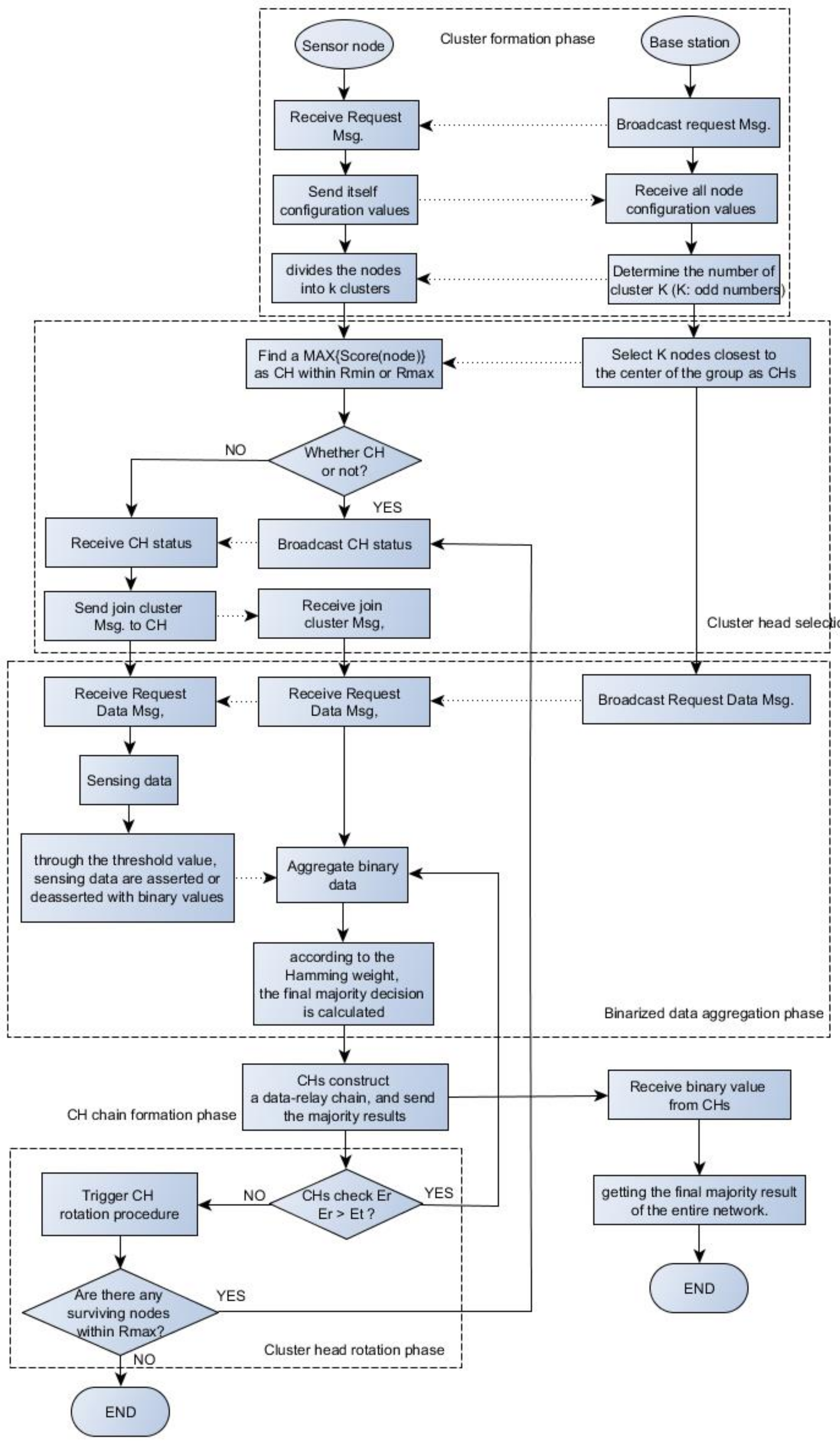In addition, the k value is specially designed to define the appropriate number of clusters (most of which are odd numbers) as the majority decision of each cluster data, and the final result is transmitted to the BS. Furthermore, we considered that the spatial correlation between the nodes prevents redundant transmissions. Our study is categorized into the following phases: cluster formation, CH selection and rotation, the majority result of a binarized aggregation, and the CH chain formation phase. In the following section, we discuss the working principle of our proposed EEBDA scheme in detail, and the overall operation of the proposed method is depicted in Figure 6 (flowchart).

Table 1. Notation and definition.

Notation	Definition
$d_0$	distance threshold based on the first-order radio model
K	the number of clusters
$n_k$(x)	the nodes x in cluster {1, …, K}
Et	energy threshold for CH rotation
Er	the residual energy
Ein	the initial energy
Gxy	location of the group center
D($n_k$(x))	Euclidean distance between $n_k$(x) and Gxy
Rmin	scanning range at given cluster center with radius 10 m
Rmax	scanning range at given cluster center with radius 25 m
$C_{k\in \left\{1,\dots , k\right\}}$	cluster {1, …, K} of the deployed area
$C{H}_{k\in \left\{1,\dots ,k\right\}}^{maj}$	the final majority value of cluster {1, …, K}
$C{H}_k$	cluster head {1, …, K}
$B{n}_k^{C_k}\left(x\right)$	a binary value of node x in cluster {1, …, K}
BSmaj	the final majority value of a BS

lists the notations and definitions used in this study.

3.1. Cluster Formation

There are different assumptions about the radio characteristics, including energy dissipation in the transmission and reception nodes. This study adopts a simple model, and the following parameter values reference the first-order radio model [19]. In Equations (3) and (4), the amplifier parameters are used to calculate the distance threshold (d₀) of data transmission and reception between two nodes. Where $d_0=\sqrt{\left({\epsilon }_{fs}/{\epsilon }_{mp}\right)}\cong 87.7058$, d₀ = 87, simplifying the calculations to cut off the decimal points and take the distance threshold as an integer value of 87. At the beginning of the cluster formation, neighboring nodes were grouped into the same clusters using k-means++ clustering. Equation (6) is used to calculate the k value of k-means++, which is used to divide the cluster into k groups, as shown in Figure 7. In addition, the k value is defined as an odd value for the subsequent calculation of the majority decision making. In Equation (6), C is the length and width divided by d₀ individually and takes the ceiling value. If C is odd, then k = C; if C is even, then k = C + 1.

$$C=\lceil \frac{length}{d_0}\rceil \times \lceil \frac{width}{d_0}\rceil \mathrm{then} k=C+M$$

$$\mathrm{where} M=\left\{\begin{array}{c}0, C is odd\\ 1, C is even\end{array}\right.$$

(6)

In Figure 7, “length” denotes the length of the sensing range, and “width” denotes the width of the sensing area. For example, assume that k equals five; it is divided into a schematic diagram of five clusters.

3.2. Cluster Head Selection and Rotation

A CH rotates among the nodes and attempts to equilibrate the energy usage through all nodes. Therefore, the CH selection will affect the lifetime of a WSN because a CH consumes more power than an ordinary (non-CH) node. The monitoring, aggregation, and control of each cluster are performed by the CH, which acts as a leader. The cluster heads have a direct transmission with the BS. In the initial phase, the cluster head selects the node with the maximum residual energy, and more than the energy threshold (E_t), and is closest to the group center as the cluster head. Other nodes then join the nearest cluster head, and their probability of being selected as the cluster head increases the next time. The CH rotation aims to show the advantages of being cluster based and selecting a plentiful energy sensor node to be a CH in a cluster; the energy load can be dispersed in the cluster. In this study, a threshold value of the residual energy was considered when selecting the CHs in each subsequent round. The nodes near the cluster head dissipate less energy as the relay data of these nodes is a shorter distance. Likewise, more energy is consumed if the nodes are far away from the CH. If the current CH energy is less than the energy threshold, it triggers the rotation CH procedure, where the energy threshold (E_t) is the overall average residual energy of a cluster in which the current CH is located. Equation (7) shows that the node with the highest score in each cluster is selected as the CH. In Algorithm 1, R_min and R_max denote the scanning range with a radius of 10 m and 25 m, respectively [35]. Any nodes beyond the R_max range are already far from the cluster (group) center and are not ideal candidates as CHs. The process of accessing the nearest nodes from the group center and finding a node with the maximum residual energy uses Algorithm 1 at each rotation CH phase.

$$Score\left(n_k\left(x\right)\right)=\frac{E_r{n}_k\left(x\right)}{E_{in}{n}_k\left(x\right)}+\frac{1}{D{\left(n_k\left(x\right)\right)}^2}$$

(7)

where$E_{re}{n}_k\left(x\right)$and $E_{in}{n}_k\left(x\right)$are the residual and initial energies of node x, respectively, and $D\left(n_k\left(x\right)\right)$is the distance between node x and the center of the group.

Algorithm 1 Cluster head rotation

Input: Rmin, Rmax, Gxy, CHk, $n_k$(x), Et, Er Output: New_CHk For each node $n_k$(x) in {1, 2, …, K}  IF CHk.Er <= Et//Check if the residual energy of the current CHk is less than or equal to the energy  threshold (Et).    Scan Gxy.radius = Rmin//Scanning all nodes in the 10 m radius of a group center   IF Find a MAX{$Score\left(n_k\left(\mathrm{x}\right)\right)$}//Find the node with maximum residual energy, ref Equation (7)    Broadcast New_CHk = $n_k\left(x\right)$ selected    ELSE    Scan Gxy.radius = Rmax//Scanning all nodes in the 25 m radius of a group center     IF Find a MAX{$Score\left(n_k\left(x\right)\right)$}      Broadcast New_CHk = $n_k\left(x\right)$ selected     ELSE      IF Random selection of a MAX{$Score\left(n_k\left(\mathrm{x}\right)\right)$}       Broadcast New_CHk = $n_k\left(x\right)$ selected      END IF     END IF    END IF  ELSE   The CHk to continues as the CH  END IF END FOR

3.3. The Majority Result of a Binarized Aggregation

All sensor nodes are designed to perform omnidirectional sensing and sense events within a certain radius. Due to low cost and energy constraints, multiple sensor nodes are required to be densely deployed in a domain of interest to perform a common sensing task, which leads to highly correlated data transmission [36,37]. Notably, the communication between nodes consumes more energy than computation [15]. For dense WSNs, multiple nodes detect the same event simultaneously when the number of nodes exceeds the minimum data resolutions required for the sensing area. The correlated data transmissions cause unnecessary collisions and consume additional energy. 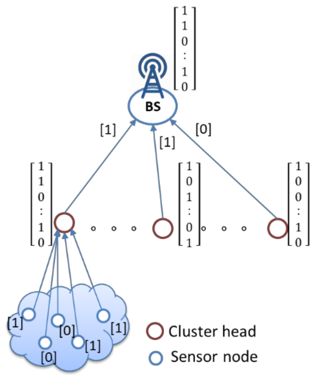Therefore, data aggregation for energy efficiency considerations is a critical task in clustered sensing networks [38]. Moreover, a significant amount of energy saving can be taken advantage of by spatial correlation and further binarized data. The cluster head is responsible for collecting data sensed by non-CH nodes and passes this binarized data to a BS. The BS broadcasts a data request message, and all sensor nodes transmit binary sensing data to their CH. The energy consumed to relay one bit of data is equivalent to that consumed when executing several hundred instructions. Therefore, communication must be managed according to the properties of the network to solve the problem of what to do with multi-hop relay data and redundant data transfer by all means.

Furthermore, the idea of this study is a constraint that can be built from multiple constraints by simply using the “AND” and “OR” operators (that is, “1” and “0” bit values). First, the collected sensing data are asserted (asserted/deasserted) with binary values of one or zero at the sensor nodes through a threshold value and then sent to their CH. For example, assume that the threshold value for humidity is 30%. IF node A = “humidity’’ <= 30 THEN node A’s asserted value is 1. This means that the humidity value sensed at the node is too low, the environment is too dry, and crops need watering. CH calculates the Hamming weight of the binary value from all nodes within a cluster; decisions with a majority rule then send majority decision result of a 1-bit or 0-bit value to the BS. In the final phase, the BS also uses the Hamming weight to calculate the binary values from all CHs to obtain the final majority result. Suppose C_k has a number of members n_k(1), n_k(2),…,n_k(x) with binary decisions $B{n}_k^{C_k}\left(1\right)$, $B{n}_k^{C_k}\left(2\right)$,…, $B{n}_k^{C_k}\left(x\right), k\in \left\{1,\dots ,k\right\}$ as given in Equation (8), where $C{H}_{k\in \left\{1,\dots ,k\right\}}^{maj}$ denotes the majority result of each CH in the network. The final majority result of the entire network ($\sum B{S}^{maj}$) can be determined by Equation (9). Finally, the pseudo-code of the network’s final majority result algorithm is presented in Algorithm 2. An illustration is shown in Figure 8, where the one-dimensional matrix represents binarized aggregation data and then computes the Hamming weight in each matrix to obtain the majority result.

$$\sum C{H}_{k\in \left\{1,\dots ,k\right\}}^{maj}=\left\{\begin{array}{c}1 if \left|\left\{x\right|B{n}_k^{C_k}\left(x\right)=1\}\right| \ge \left|\left\{x|B{n}_k^{C_k}\left(x\right)=0\right\}\right| \\ 0 otherwise\end{array}\right.$$

(8)

$$\sum B{S}^{maj}=\left\{\begin{array}{c}1 if \left|\left\{k\right|C{H}_{k\in \left\{1,\dots ,k\right\}}^{maj}\left(k\right)=1\}\right| \ge \left|k|\left\{C{H}_{k\in \left\{1,\dots ,k\right\}}^{maj}\left(k\right)=0\right\}\right| \\ 0 otherwise\end{array}\right.$$

(9)

Algorithm 2 Find the majority result of a cluster

Input: $C_{k\in \left\{1,\dots ,k\right\}}$, CHk, $n_k$(x),$B{n}_k^{C_k}\left(x\right)$, Output: Majority result of a cluster ($\sum C{H}_{k\in \left\{1,\dots ,k\right\}}^{maj}$) For each node $n_k$(x) in $C_{k\in \left\{1,\dots ,k\right\}}$    $C{H}_{k\in \left\{1,\dots ,k\right\}}=\left\{B{n}_k^{C_k}\left(x\right)\right\}$    //each cluster head (CHk) receives binary values from its own member nodes $B{n}_k^{C_k}\left(x\right)$     IF $\sum C{H}_{k\in \left\{1,\dots ,k\right\}}^{maj}=1$    //where $\sum C{H}_{k\in \left\{1,\dots ,k\right\}}^{maj}$ can be calculated by using Equation (7).     Send $C{H}_{k\in \left\{1,\dots ,k\right\}}^{maj}=1$ to BS//Send cluster final majority result one value to the BS    ELSE    Send $C{H}_{k\in \left\{1,\dots ,k\right\}}^{maj}=0$ to BS    END IF     $B{S}^{maj}$ = {$C{H}_{k\in \left\{1,\dots ,k\right\}}^{maj}\left(k\right)$} //BS receives binary values from $C{H}_{k\in \left\{1,\dots ,k\right\}}^{maj}$     IF $\sum B{S}^{maj}=1$     //where $\sum B{S}^{maj}$ can be calculated by using Equation (8).      final majority result of the entire network is true     ELSE      final majority result of the entire network is false     END IF End For

3.4. CH Chain Formation Phase

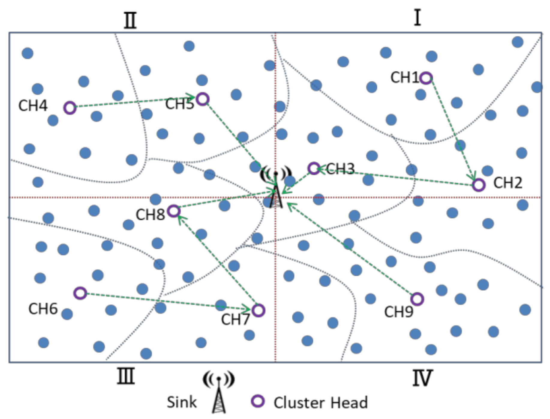
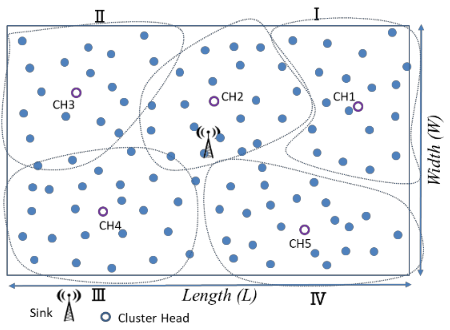
For the CH chain formation phase, the center of the entire sensing area is used as the origin to divide into four logical quadrants, and it is assumed that the BS is located in the center of the sensing area. The CHs in the same quadrant construct a data-relay transmission chain, and the CH of the closest BS is fixed at the chain-end for communication with the BS. The CHs transmit the cluster’s majority decision results to the BS, as shown in Figure 9. There are K cluster heads in this study, and each cluster head is assigned a unique random number from 1 to K, where K is the number of clusters and K is the odd number. To avoid CHs closer to the BS, more data must be relayed. The CH is located in the same quadrant, from the farthest CH and nearest CH to the BS as the chain head and chain tail, constructing a data transmission chain. The CH nodes in each chain transmit data to their chain tail node. Consider the third quadrant in Figure 9. For example, there are three cluster heads, CH6, CH7, and CH8, in quadrant 3. The farthest from the BS, CH6 is the beginning of a chain node and ends at the nearest cluster head (CH8), forming a communication chain. Finally, CH8, CH9, CH3, and CH5 forward the aggregated binarized data toward the BS.

3.5. Overhead Cost Analysis

In the proposed EEBDA method, overhead cost analysis is mainly divided into majority decision part and data aggregation. For data aggregation, after CHs receive a BS data request message (a request message), all nodes send a binary value to CH by threshold asserting/deasserting. The node sends data to CH within one hop. The CHs construct a chain, which also sends data to the BS within three hops. Assuming that there are n nodes in each cluster, each CH receives n binary values. If the network has k clusters, the BS will receive k binary values from the CH. As a result, the total number of messages per round is M_total = k × n. The binary value is transmitted to the CH through the sensor nodes in the majority decision part, and the CH stores binarized aggregation data in the one-dimensional matrix to perform Hamming weight operations. Therefore, the time complexity is O(n), and no additional space is consumed; hence, the space complexity is O(1) [12,39].

4. Experimental Analysis

In this section, we evaluate the performance of the proposed EEBDA. First, the proposed mechanism was experimented with and simulated using the MATLAB simulation tool [40]. Second, all experiments were executed on a single machine running Windows 10 with an Intel Core i7-7700 CPU @ 3.60 GHz.

4.1. Experiment Setting

We compared EEBDA with LEACH, LEACH-C, and DEEC algorithms for performance analysis. Therefore, all four protocols are simulated for comparative analysis, where nodes are randomly deployed 100, 200, and 500 nodes in a WSN environment. All nodes possess the same initial energy. The parameter settings used in the simulations are listed in

Table 2. Simulation parameters.

Parameters	Values
Size of the WSN	100 m2, 200 m2
Number of sensor nodes	100, 200, and 500
Position of BS (m, m)	(50, 50), (100, 100)
Packet size	4000 bits
Initial energy (E0)	0.5 J
Energy for data aggregation	5 nJ/bit/signal
Deployment type	Random deployment
Energy model	First-order radio model

.

We evaluated the energy consumption of WSNs as it is a major limitation. These simulation experiments aimed to evaluate the effectiveness and efficiency of the protocols. Furthermore, several metrics were used to compare them, such as the average residual energy of the network, the number of nodes alive, and the variance of the residual energy. Finally, we performed experiments on three metrics to compare the EEBDA with the other protocols.

4.2. The Energy Consumption Performance

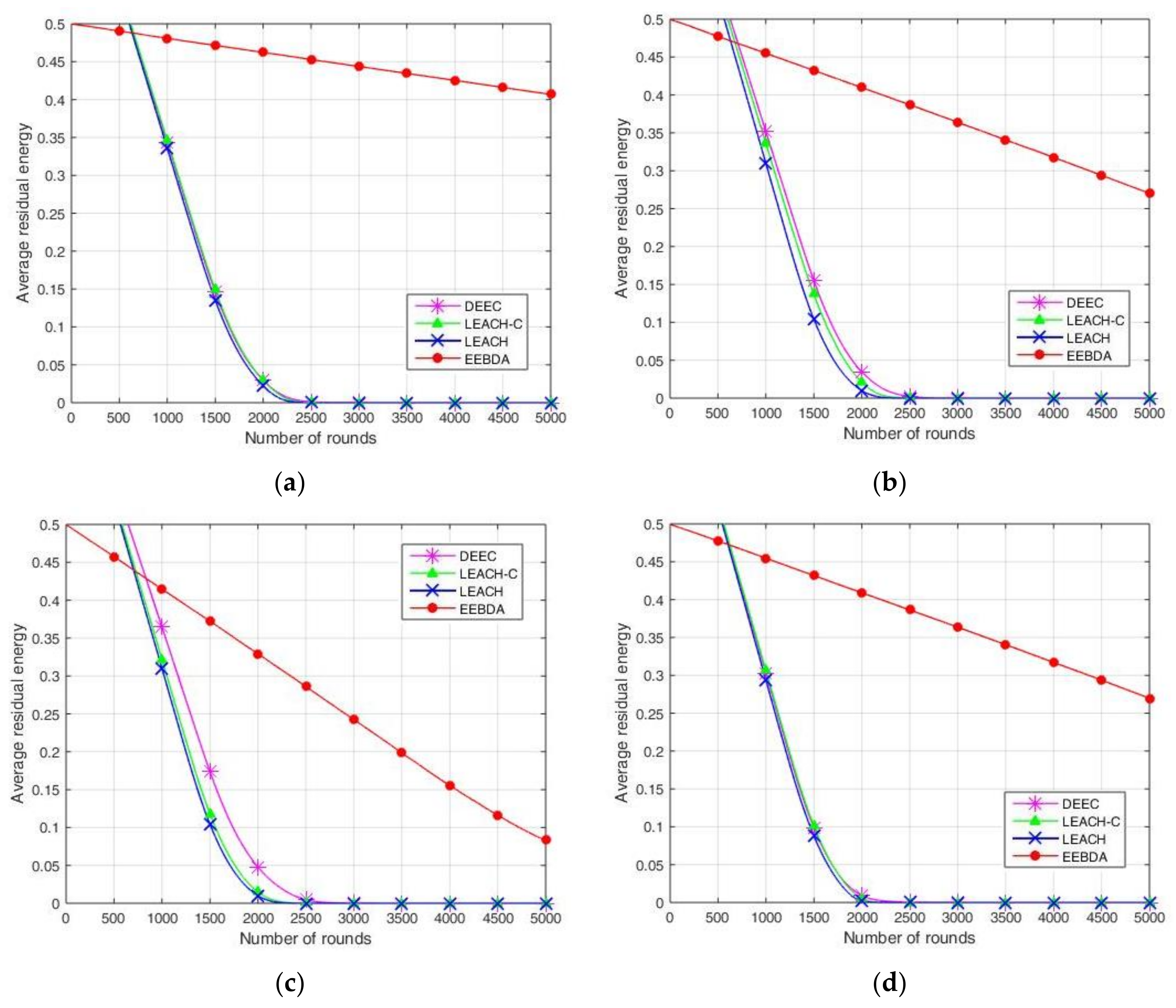
A comparison of the network average residual energy concerning time (in rounds) is shown in Figure 10. In the parameter setting for initial energy, 0.5 J energy is assigned to each node, where the total energy of the network is 50, 100, and 250 J for 100, 200, and 500 nodes, respectively. The simulation parameters of the network are presented in Table 2. The 100, 200, and 500 sensor nodes were randomly deployed in regions of size 100 m² and 200 m², respectively.

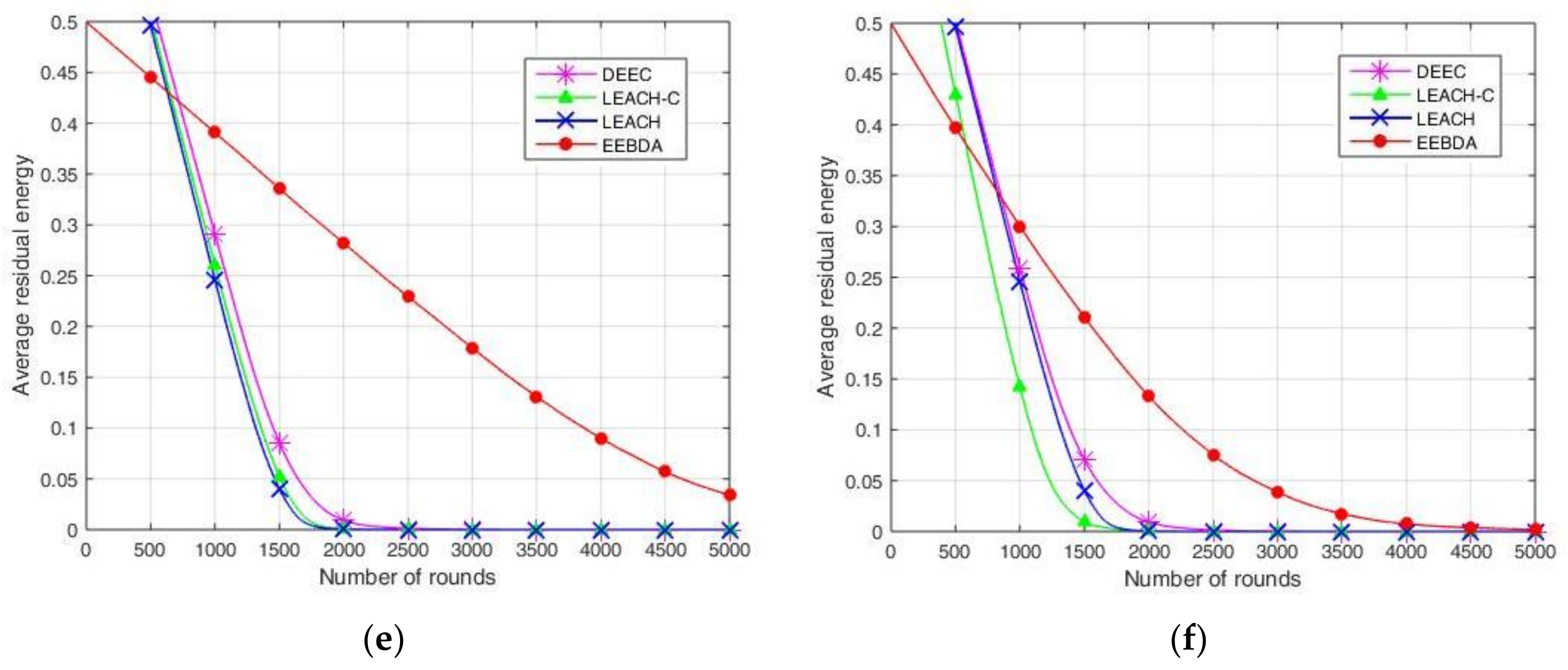
As illustrated in Figure 10, the residual energy of the sensor nodes is compared after multiple simulations run over LEACH, LEACH-C, DEEC, and EEBDA in WSNs. The total residual energy of the network considers the residual energy of all the nodes in each round. This metric is reported in Figure 10, which shows that the proposed scheme (EEBDA) saves more energy than the other protocols. In Figure 10, the maximum number of rounds is 5000; as shown in the figure, the average residual energy in the WSN varies with the number of rounds. For example, when the number of rounds is approximately 2250, the average residual energy of the other three algorithms is approximately zero. We considered the distance between the sender and receiver, the cluster size, and the spatial correlation among sensor nodes. Therefore, the EEBDA scheme has a lower energy consumption than the other algorithms, and the proposed scheme can prolong the lifetime of a WSN. It is clearly shown in the Figure that the energy dissipation of the proposed protocol is less than that of all the other schemes.

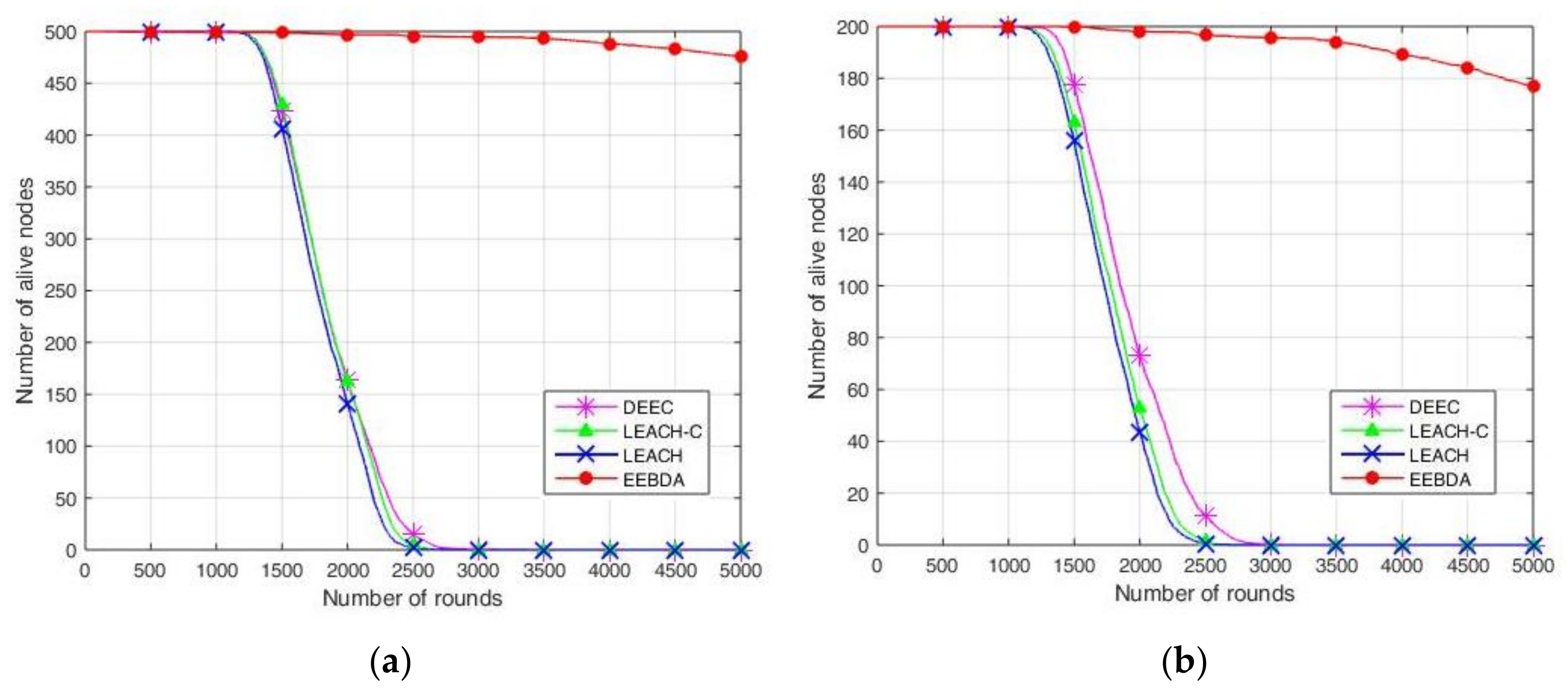
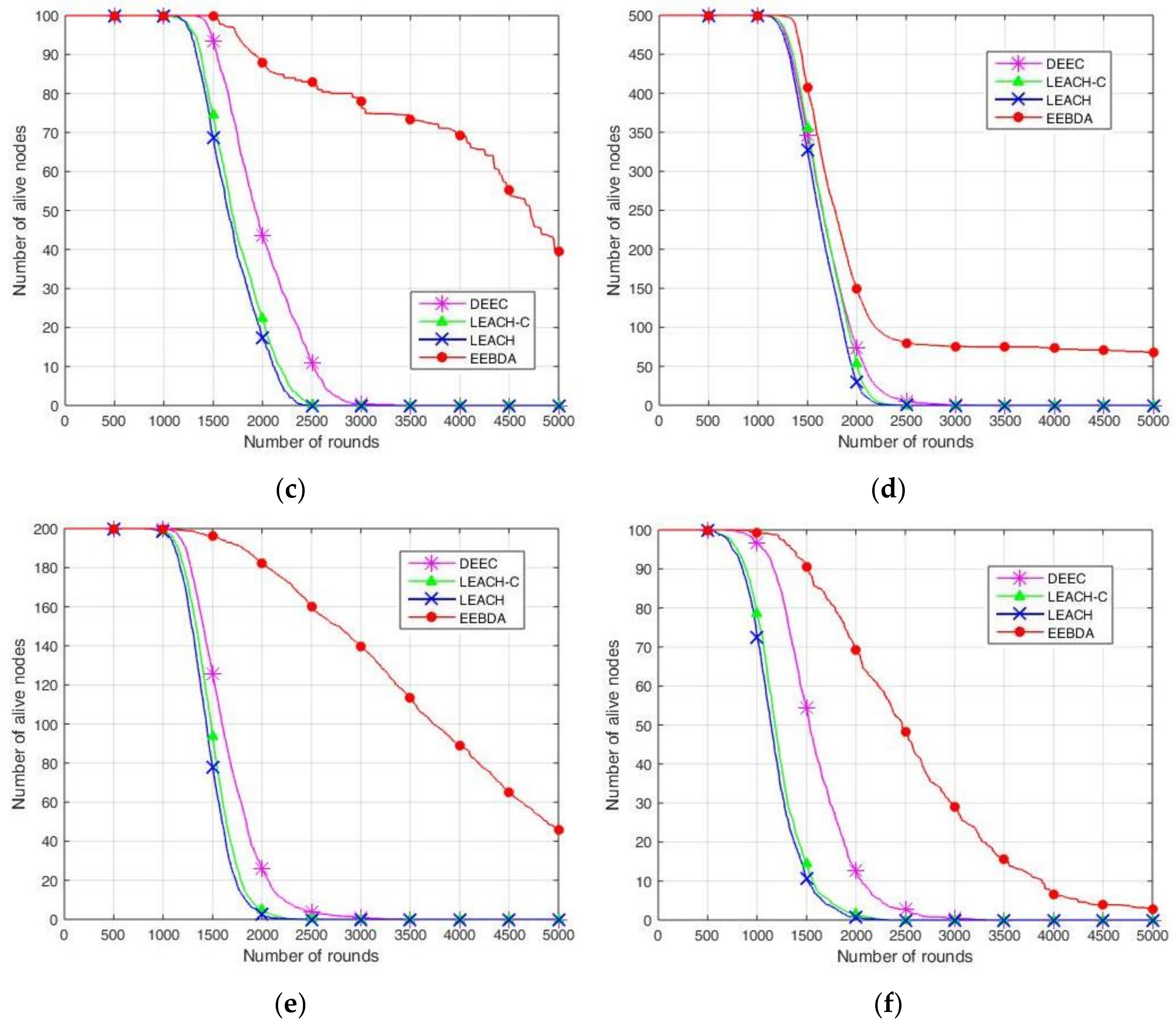
To evaluate the proposed EEBDA algorithm more accurately, we compared it again with LEACH, LEACH-C, and DEEC from surviving sensor nodes. In Figure 11, the results show the number of surviving sensor nodes after 5000 rounds; the sensing area is 100 m² and 200 m², and the number of network nodes is 100, 200, and 500 for LEACH, LEACH-C, DEEC, and EEBDA.

The surviving sensor nodes of the WSN consider the alive nodes in each round. This simulation result is reported in Figure 11, which shows more alive nodes in our proposed method (EEBDA) than in the other protocols. In Figure 11, 100, 200, and 500 nodes deployed randomly are reported to be almost zero at about round 2000 on LEACH, LEACH-C, and DEEC. Thus, in our proposed method, the network lifetime is significantly better than the other algorithms in all cases. As expected, our scheme determines the network configuration that consumes the lowest energy in every round. Therefore, the surviving nodes of the network are higher than those obtained with LEACH, LEACH-C, and DEEC. From the Figure, we can conclude that EEBDA realizes the lowest energy consumption and prolongs the lifetime of the network.

4.3. The Variance of the Residual Energy

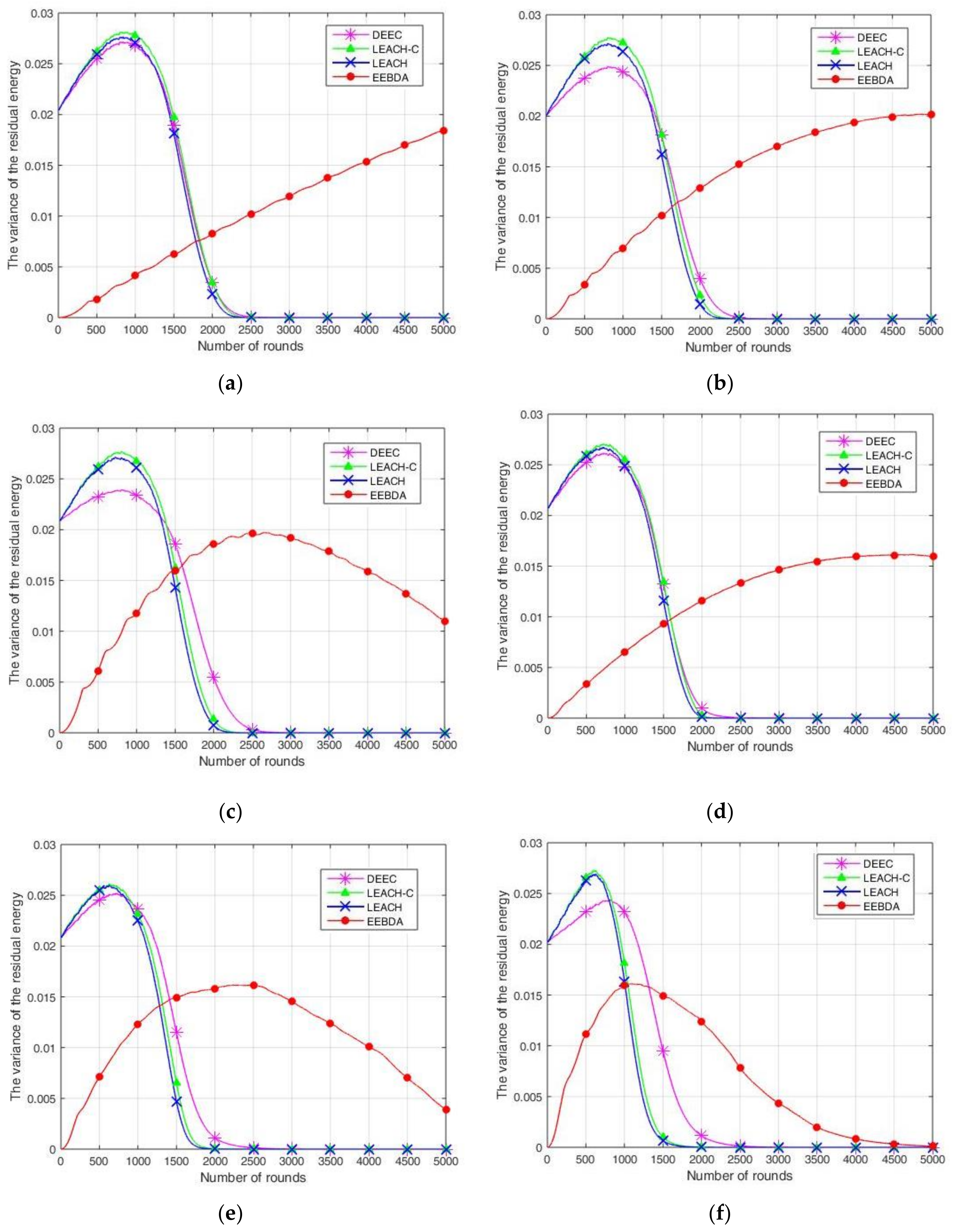
The unbalanced energy consumption affects the network lifetime and leads to an unbalanced energy consumption in nodes. In addition, the premature death of some nodes reduces the overall performance of the WSN. In addition, it results in significant differences in the death time of the nodes in the WSN, which adversely affects the stability of the network and the efficiency of the transmission of information. Figure 12 mainly reflects the energy consumption balance in the remaining surviving sensor nodes in the network with high network operation times. In this work, we have made an experimental simulation variance of the residual energy to demonstrate this problem to compare the difference in the number of nodes and sensing area among the algorithms. As shown in Figure 12, the variance of the residual energy of each node is smaller than that of the other three algorithms when using EEBDA. This means that the energy consumption of each node is more balanced, and it is more conducive to improving the overall practical lifetime of the WSN.

5. Discussion

The EEBDA outperformed the LEACH, LEACH-C, and DEEC protocols in the lifetime of the network, energy consumption, and energy balance. The reasons are summarized as follows.

LEACH, LEACH-C, and DEEC protocols define different threshold values of the CH selection. In LEACH and DEEC, the CH’s selection is random. These results cause an imbalanced distribution of CH in each round, which causes an imbalance in energy consumption among nodes and the premature death of some nodes. In DEEC, some adjustments are made for CH selection such that high-energy nodes have a higher probability of becoming CH than low-energy nodes. However, the main weakness of DEEC is the overhead involved in handling the average energy of the entire network. This results in faster death of high-energy nodes, which prolongs the instability period of the network and imbalanced energy consumption among nodes. In the probability of electing CHs, the LEACH-C protocol that selects CHs considers the average energy of the nodes. In other words, when the residual energy of a node is higher than the average energy of the network, the average probability of that node being elected as CH is higher than that of a node whose residual energy is less than the average energy of the network. Therefore, compared to LEACH, the difference in energy consumption between advanced and ordinary nodes decreases, and the network lifetime is more prolonged than LEACH. In the CH selection model, LEACH-C applies the residual energy and the average energy of the network to the defined threshold compared to DEEC. When the residual energy is higher than the average energy of the network, the node has a higher probability of being elected as CH; however, it remains slightly random. Therefore, the lifetime of the network is improved relative to the DEEC protocol; however, there is no more significant improvement in the residual energy variance than LEACH and LEACH-C.

Conversely, our algorithm uses the Hamming weight to calculate the majority results by the sensing data asserted/deasserted with binary values of one or zero through a threshold value. The data-relay chain of CH considers the distance from the CH to the BS and overcomes the transmission of redundant data. Our algorithm considers that the search range of CH selection is located as near as possible from the group center, reduces the energy consumption in unnecessary transmission, saves network energy consumption, and prolongs the lifetime. Therefore, EEBDA is superior to LEACH, LEACH-C, and DEEC protocols concerning energy consumption and lifetime. The proposed EEBDA mechanism, with binarized data aggregation afterward, achieved a majority decision that utilizes spatial and symmetry data correlation in the sensor data that can be used to reduce the energy consumption of sensor nodes for persistent data collection and maximize the lifetime of the network.

6. Conclusions and Future Works

According to the aforementioned simulated results, the evidence of spatial correlation chain-clustering in the EEBDA binarized data aggregation mechanism is superior to LEACH, LEACH-C, and DEEC protocols in terms of the residual energy of sensor nodes and the network lifetime. To further improve the performance of WSNs, this study proposes a novel WSN clustering routing protocol. First, the binarized data aggregation technique is introduced based on a simple energy consumption model. Subsequently, the k-means++ clustering algorithm determines the K value as an odd value to set the number of clusters to judge the majority decision. The CHs first construct a data-relay chain with CHs in the same quadrant, construct a data-relay chain with neighboring CHs, and send their clusters’ final majority results to the BS. The CHs check their residual energy at the end of each round, which decides whether or not to rotate the CH to balance the energy consumption within the cluster. In cluster-based WSNs, there is a mode of asymmetric data transmission from sensor nodes to the CH, allowing sensor nodes to report sensed data in turn, maximizing the network lifetime. However, our protocol has some shortcomings.

First, even if the node energy is sufficient, faulty nodes or transmission failures may occur because of the uncertainty of the natural environmental factors in the data transmission process. Therefore, in future works, we can consider adding a fault-tolerant mechanism to allow a few faulty nodes, in tandem with mostly healthy nodes, to execute data transmission tasks and keep network operation. Second, the protocol applies only to two-dimensional or land scenarios. We did not consider three-dimensional or underwater scenarios; typically, sensor nodes may be deployed in three dimensions, and robust communication protocols should be considered to avoid interference. Therefore, in the future, we will consider proposing a clustering routing protocol based on this protocol that is suitable for three-dimensional scenarios with energy efficiency.