Article

The Double Phospho/Dephosphorylation Cycle as a Benchmark to Validate an Effective Taylor Series Method to Integrate Ordinary Differential Equations

by
Alessandro Borri
1,*,
Francesco Carravetta
1 and
Pasquale Palumbo
2
1
Institute for Systems Analysis and Computer Science “A. Ruberti”, National Research Council of Italy (CNR-IASI), 00185 Rome, Italy
2
Department of Biotechnology and Biosciences, University of Milano-Bicocca, 20126 Milan, Italy
*
Author to whom correspondence should be addressed.
Symmetry 2021, 13(9), 1684; https://doi.org/10.3390/sym13091684
Submission received: 30 July 2021 / Revised: 6 September 2021 / Accepted: 8 September 2021 / Published: 13 September 2021

Abstract

:
The double phosphorylation/dephosphorylation cycle consists of a symmetric network of biochemical reactions of paramount importance in many intracellular mechanisms. From a network perspective, they consist of four enzymatic reactions interconnected in a specular way. The general approach to model enzymatic reactions in a deterministic fashion is by means of stiff Ordinary Differential Equations (ODEs) that are usually hard to integrate according to biologically meaningful parameter settings. Indeed, the quest for model simplification started more than one century ago with the seminal works by Michaelis and Menten, and their Quasi Steady-State Approximation methods are still matter of investigation nowadays. This work proposes an effective algorithm based on Taylor series methods that manages to overcome the problems arising in the integration of stiff ODEs, without settling for model approximations. The double phosphorylation/dephosphorylation cycle is exploited as a benchmark to validate the methodology from a numerical viewpoint.

1. Introduction

Protein phosphorylation is a ubiquitous regulatory mechanism for cells, generally working to activate or inactivate molecules [1]. From a biochemical viewpoint, to phosphorylate a molecule consists in the binding of a phosphoryl group P O 4 [2]. The general model to deal with phosphorylation is to exploit the framework of enzymatic reactions, where the substrate M is supposed to be modified (phosphorylated, actually) into the product M p by means of the preliminary formation of a complex C provided by the binding of an enzyme (called kinase, K) in charge to catalyze the phosphorylation, see the scheme in (1).
M + K k 1 k 1 C k k 2 M p + K
Phosphorylations usually introduce conformational changes that activate/inactivate the enzymatic activity of a protein, or simply prime degradation processes, like the ones involved in the yeast cell cycle (see, e.g., in [3,4] dealing with the degradation of Sic1 and Whi5, respectively) or those involving tyrosine kinase pathways, regulating diverse cellular processes, and whose dysregulation is one of the leading causes of cancer progression [5]. In many important cases, multi-site phosphorylations are required to ensure the correct timing of activation [6,7]. Besides, according to specific conditions and biological frameworks, phosphoryl groups can be removed, making phosphorylation a reversible activation/inactivation mechanism. Moreover, in this case the dephosphorylation may be treated as a generic enzymatic reaction, with the enzymes that catalyze the reaction called phosphatases P:
M p + P h 1 h 1 C p h 2 M + P
Combinations of multiple phosphorylations/dephosphorylations have been selected by nature as devices, providing specific useful biological functions. Within this framework, the Double Phosphorylation/Dephosphorylation Cycle (DPDC) is a symmetric network motif consisting of a double reversible phosphorylation step required to activate a given substrate M:
M + K k 11 k 11 C 1 k 12 M p + K M p + K k 21 k 21 C 2 k 22 M p p + K M p p + P k 31 k 31 C 3 k 32 M p + P M p + P k 41 k 41 C 4 k 42 M + P
where the final product is the doubly phosphorylated M p p . Ordinary Differential Equation (ODE) models of DPDC use to combine in a symmetric fashion the four enzymatic reactions [8], providing a bistability regime where the non-phosphorylated or the double-phosphorylated versions of the substrate is predominant [9]. A primary motivation in investigating the computation of the system solutions is that, in a recent paper [10], it has been proven that symmetry breaking in the dynamical solutions of such a network may lead to modify its emergent properties, including concentration robustness of different stationary solutions.
In this context, numerical integration of enzymatic reactions in ODE form has been a matter of investigation for more than a century [11,12], since the seminal works of Michaelis and Menten [13] providing an approximation (the celebrated Quasi Steady-State Approximation (QSSA) [14]) to cope with the double time scale arising whenever biologically meaningful parameters are assigned. Multi-timescale phenomena are very common in biology, see, e.g., the very recent cardiac cell model in [15].
Indeed, in enzymatic networks, the binding/unbinding reactions use to occur at a faster rate, thus leading to stiff ODEs, thus characterized by numerical instability when ordinary numerical schemes are employed for their integration. In particular, in the case of stiff equations, ad hoc integration methods, like the one illustrated in [16] for linear multistep methods, can be employed to approximate the solution efficiently. Like any approximations, there are limitations that may render unfeasible its concrete applicability. Indeed, in [17] we showed how the numerical integration of a basic enzymatic reaction model may create serious problems even to well established procedures like the ones implemented by Matlab in ode45 and ode15s functions. Besides, things become even more crucial in the DPDC, as it has been shown in [18] how the QSSA may miss the bistability property.
In order to deal with stiff ODEs, Taylor Series Methods (TSMs) can be used. These methods build up a polynomial approximation (up to some fixed order k) of the ODE solution around the initial point through Taylor series expansion, which amounts to the recursive calculation of the partial derivatives of the ODE function at the initial point, up to the order k. With respect to standard Runge–Kutta methods, TSMs do not exhibit worse performance in terms of numerical stability, and guarantee a better accuracy in the solution calculation for higher degrees of the approximating polynomial. We refer the interested readers to the works in [19,20,21,22,23] for an in-depth description of TSMs and their numerical properties.
The main issue with TSMs is that, as the approximation order k increases, the calculation of all the required derivatives becomes too cumbersome, and some preliminary transformations need to be applied to the original problem in order to simplify the derivatives calculation. To this end, in the present work, we employ some recent technical results published in [24,25], according to which ODE systems can be embedded into higher-order quadratic equations which, in spite of their dimensionality, allow for more efficient differentiation, which in turn can be exploited for numerical integration via TSM. These results have been already exploited in [17] for the class of simple enzymatic reactions (two differential equations), and are here extended to the more challenging DPDC case (seven differential equations). Simulations are promising as the numerical results show a higher qualitative accuracy of the method with respect to standard off-the-shelf solvers for an appropriate choice of the reaction parameters which make the equations stiff.
The paper is organized as follows. Section 2 reviews the methods involving quadratization and approximate integration of a class of differential equations. Section 3 adapts the framework to the context of Double Phosphorylation/Dephosphorylation Cycle. Section 4 provides some numerical simulations of the DPDC system. Finally, Section 5 offers concluding remarks and ideas for further developments.

2. Exact Quadratization and Approximate Integration of σ π Differential Equations

This section recollects and adapts some results mainly developed in [24,25] for more general classes of dynamical systems than those developed in this work. Except where differently specified, we adopt the following vector and indices convention: a vector v is always a column vector, and v is its transpose. With respect to indices, given a vector v, the scalar v j denotes its j-th entry; instead, in case of double subscripts, like in Z i , j , when dealing with a vector we mean a nested notation, where Z i , j is the j-th scalar/vector component of vector Z i , and vector Z i is the j-th vector component of vector Z; on the other hand, when dealing with a matrix, Z i , j refers to the usual scalar entry in row i and column j.

2.1. Exact Quadratization of σ π -ODEs into Driver-Type Differential Equations

We consider a first-order ODE system
x ˙ = f ( x ) , x R n ,
where the function f is a formal polynomial of x, i.e., a polynomial writing where the exponents are allowed to be any real number. More formally, the components of f are in the form
f i ( x ) = l = 1 ν i v ¯ i , l X i , l ( x ) ; X i , l ( x ) = r = 1 n x r p i , r l ,
where p i , r l are real exponents, the ν i quantities X i , l in (5) are named monomials and v ¯ i , l are real coefficients. We refer to this kind of functions as σ π -functions, and to the associated system of differential equations as σ π -ODE.
For σ π -ODEs, the following theorem holds, by virtue of which the system (4) and (5) can be densely embedded in a higher-dimensional quadratic system.
Theorem 1.
(Exact Quadratization Theorem, adapted from the work in [24]). Any σ π -ODE in the form (4) and (5), with domain V I R n , is quadratizable on the non empty, open and dense subset U = V S (with S denoting the set of all coordinate hyperplanes in R n ), and the quadratization is given by the following homogeneous Riccati equation in the indeterminates x i and Z i , l :
x ˙ i = ( v ¯ i Z i ) x i
Z ˙ i , l = r = 1 n π i , r l ( v ¯ r Z r ) Z i , l
where π i , r l = p i , r l δ i , r , and δ i , r being the Kronecker symbol: δ i , r = 1 (resp: δ i , r = 0 ) if i = r (resp: i r ).
It clearly appears that the specific Riccati equation constituting the quadratization (6) and (7) includes the original state variables, so it is possible to define an augmented state such that the original ODE system (4) is now embedded in the following extended system evolving in R m , with m n :
x i ˙ = i = 1 m v i , j x i x j = ( v i x ) x i ,
where, with a little abuse, we keep the notation of x for a vector now living in R m , with the first n components provided by the n components of vector x in (4), and the other m n components provided by vector Z in (7). The coefficients v i , j are suitable linear functions of the coefficients v ¯ i , l in (5). Equation (8) is called ‘Driver-type’ ODE form, while the matrix V R m × m collecting the entries v i , j , i , j = 1 , , m , is called ‘frame’.
The interested reader is referred to the works in [24,25] for further notation (including multi-indices), technical details and full proofs.

2.2. Approximate Taylor Series Integration Method

With a slight abuse of notation, let t x ( t ) be the solution of (4) with initial condition x ( t 0 ) , and consider the Taylor expansion of a generic scalar component x i ( · ) with respect to the initial time instant t 0 :
x i ( t ) = k = 0 c k ( i ) ( t t 0 ) k k ! , c k ( i ) = x i ( k ) ( t 0 ) .
Numerical integration techniques based on the application of the truncated series in (9) to compute a solution of (4) are called Taylor Series Methods (TSMs). Unfortunately, such a series expansion cannot be straightforwardly applied to compute the solution for general systems as it requires the explicit computation of the derivatives of the solution at the initial point, which usually reveals to be too cumbersome. Below is reported a Theorem that allows to compute the coefficients of the Taylor expansion for a system in the ‘Driver-type’ ODE form (8).
Theorem 2.
(from [25]). Consider a ‘Driver-type’ ODE in the form (8). Then, the coefficients c k ( i ) , k > 0 , in the Taylor expansion (9) are given by
c k ( i ) = i 1 , , i k S v i , i 1 , , i k k + 1 · x i ( t 0 ) x i 1 ( t 0 ) x i k ( t 0 ) ,
where i s S = { 1 , , n } , for s = 0 , 1 , , k (we set i 0 = i ), and the (constant) coefficients v i , i 1 , , i k k + 1 , are given by the following recursive equation
v i , i 1 , , i k k + 1 = v i , i 1 , , i k 1 k j = 0 k 1 v i j , i k , v i 1 = 1 ,
where the coefficients v i , j , i , j = 1 , , m , are defined in (8).
Approximate numerical integration based on Theorem 2 can be readily performed by truncating the series (9) at a finite order k ¯ , provided that the integration formula is reinitialized frequently enough to prevent numerical instability. This readily leads to the following iteration. Let x ^ i ( j Δ ) , i = 1 , , n , for j = 0 , 1 , , be the approximate value of x i at time j Δ provided by the algorithm, where t 0 = 0 and a fixed sampling time Δ > 0 are assumed for simplicity. Then, the approximate solution at all times t 0 is given by
x ^ i ( t ) = k = 0 k ¯ c k , j ( i ) ( t j Δ ) k k ! , t [ j Δ , ( j + 1 ) Δ ) , c k , j ( i ) = i 1 , , i k S v i , i 1 , , i k k + 1 · x ^ i ( j Δ ) x ^ i 1 ( j Δ ) x ^ i k ( j Δ ) .
Note that, for k ¯ = 1 , the proposed integration scheme coincides with the forward Euler method.

3. The Double Phosphosphorylation–Dephosphorylation Cycle

According to the mass action law, the system of equations governing the dynamics of substrates and complexes in the DPDC scheme in (3) is
d M d t = k 11 M K + k 11 C 1 + k 42 C 4 d M p d t = k 21 M p K + k 21 C 2 + k 41 C 4 k 41 M p P + k 32 C 3 + k 12 C 1 d M p p d t = k 31 M p p P + k 31 C 3 + k 22 C 2 d C 1 d t = k 11 M K ( k 11 + k 12 ) C 1 d C 2 d t = k 21 M p K ( k 21 + k 22 ) C 2 d C 3 d t = k 31 M p p P ( k 31 + k 32 ) C 3 d C 4 d t = k 41 M p P ( k 41 + k 42 ) C 4
where the following conservation laws hold:
M + M p + M p p + C 1 + C 2 + C 3 + C 4 = M T ,
K + C 1 + C 2 = K T , P + C 3 + C 4 = P T .
Enzymes K and P can be replaced in (13) according to (15), so that the overall dynamics is not redundant and the system reduces to the following 7-dimensional ODE with the constraint (14):
d M d t = k 11 M ( K T C 1 C 2 ) + k 11 C 1 + k 42 C 4 d M p d t = k 21 M p ( K T C 1 C 2 ) + k 21 C 2 + k 41 C 4 k 41 M p ( P T C 3 C 4 ) + k 32 C 3 + k 12 C 1 d M p p d t = k 31 M p p ( P T C 3 C 4 ) + k 31 C 3 + k 22 C 2 d C 1 d t = k 11 M ( K T C 1 C 2 ) ( k 11 + k 12 ) C 1 d C 2 d t = k 21 M p ( K T C 1 C 2 ) ( k 21 + k 22 ) C 2 d C 3 d t = k 31 M p p ( P T C 3 C 4 ) ( k 31 + k 32 ) C 3 d C 4 d t = k 41 M p ( P T C 3 C 4 ) ( k 41 + k 42 ) C 4
Summing up all left hand sides of the system (16) yields zero, which, on the other hand, is entailed by (14), accounting that M T (the total mass) is constant over time. The algebraic equation (14) defines a six-dimensional manifold in I R 7 , invariant with respect to system (16), which means that, if one takes the initial value on this manifold, the evolution of system (16) remains on the same manifold at all times.
Remark 1.
Indeed, it can be readily proved the stronger result that the DPDC system is positive [26], as each non-positive term on the right-hand side of any equation in (16) multiplies the variable differentiated on the left-hand side of the same equation; in short, removal terms are linear in the variable of interest. This prevents the crossing of the coordinate hyperplane S already defined in Theorem 1, on which the aforementioned terms are zeroed; this will make the DPDC ODEs quadratizable (see the remainder of this section) on the same domain V I R 0 7 of the original variables, where the latter symbol denotes the non-negative orthant in I R 7 .
By setting
( x 1 , x 2 , x 3 , x 4 , x 5 , x 6 , x 7 ) = ( M , M p , M p p , C 1 , C 2 , C 3 , C 4 ) ,
it is readily seen that Equation (16) defines a σ π -ODE (see Section 2.1), with state dimension n = 7 , where the exponents in (5) are integer. As a consequence, Theorem 1 can be applied so that the system is exactly quadratized, with the quadratization that can be expressed in the ’Driver-type’ ODE form (8), with augmented state dimension m = 24 , by extending the system with the following adjoint variables, whose dynamics is defined in (7):
x 8 = x 1 1 x 4 ; x 9 = x 1 1 x 7 ; x 10 = x 2 1 x 5 ; x 11 = x 2 1 x 7 ; x 12 = x 2 1 x 6 ; x 13 = x 2 1 x 4 ; x 14 = x 3 1 x 6 ; x 15 = x 3 1 x 5 , x 16 = x 4 1 x 1 x 17 = x 4 1 x 1 x 5 x 18 = x 5 1 x 2 ; x 19 = x 5 1 x 2 x 4 x 20 = x 6 1 x 3 ; x 21 = x 6 1 x 3 x 7 x 22 = x 7 1 x 2 ; x 23 = x 7 1 x 2 x 6 x 24 = 1 .
Therefore, system (16) rewrites as follows:
x ˙ 1 = k 11 x 4 + k 11 x 5 + k 11 x 8 + k 42 x 9 k 11 K T x 24 x 1 x ˙ 2 = ( k 21 x 4 + k 21 x 5 + k 41 x 6 + k 41 x 7 + k 21 x 10 + k 41 x 11 + k 32 x 12 + k 12 x 13 ( k 21 K T + k 41 P T ) x 24 ) x 2 x ˙ 3 = k 31 x 6 + k 31 x 7 + k 31 x 14 + k 22 x 15 k 31 P T x 24 x 3 x ˙ 4 = k 11 x 1 + k 11 K T x 16 k 11 x 17 ( k 11 + k 12 ) x 24 x 4 x ˙ 5 = k 21 x 2 + k 21 K T x 18 k 21 x 19 ( k 21 + k 22 ) x 24 x 5 x ˙ 6 = k 31 x 3 + k 31 P T x 20 k 31 x 21 ( k 31 + k 32 ) x 24 x 6 x ˙ 7 = k 41 x 2 + k 41 P T x 22 k 41 x 23 ( k 41 + k 42 ) x 24 x 7
while we can use the chain rule to compute the dynamics of the adjoint variables, resulting, after some substitutions, into the following additional quadratic differential equations:
x ˙ 8 = ( k 11 x 1 k 11 x 4 k 11 x 5 k 11 x 8 k 42 x 9 + k 11 K T x 16 k 11 x 17 + ( k 11 K T k 11 k 12 ) x 24 ) x 8 x ˙ 9 = ( k 41 x 2 k 11 x 4 k 11 x 5 k 11 x 8 k 42 x 9 + k 41 P T x 22 k 41 x 23 + ( k 11 K T k 41 k 42 ) x 24 ) x 9 x ˙ 10 = ( k 21 x 2 k 21 x 4 k 21 x 5 k 41 x 6 k 41 x 7 k 21 x 10 k 41 x 11 k 32 x 12 k 12 x 13 + k 21 K T x 18 k 21 x 19 + ( k 41 P T + k 21 K T k 21 k 22 ) x 24 ) x 10 x ˙ 11 = ( k 41 x 2 k 21 x 4 k 21 x 5 k 41 x 6 k 41 x 7 k 21 x 10 k 41 x 11 k 32 x 12 k 12 x 13 + k 41 P T x 22 k 41 x 23 + ( k 41 P T + k 21 K T k 41 k 42 ) x 24 ) x 11 x ˙ 12 = ( k 31 x 3 k 21 x 4 k 21 x 5 k 41 x 6 k 41 x 7 k 21 x 10 k 41 x 11 k 32 x 12 k 12 x 13 + k 31 P T x 20 k 31 x 21 + ( k 21 K T + k 41 P T k 31 k 32 ) x 24 ) x 12 x ˙ 13 = ( k 11 x 1 k 21 x 4 k 21 x 5 k 41 x 6 k 41 x 7 k 21 x 10 k 41 x 11 k 32 x 12 k 12 x 13 + k 11 K T x 16 k 11 x 17 + ( k 21 K T + k 41 P T k 11 k 12 ) x 24 ) x 13 x ˙ 14 = ( k 31 x 3 k 31 x 6 k 31 x 7 k 31 x 14 k 22 x 15 + k 31 P T x 20 k 31 x 21 + ( k 31 P T k 31 k 32 ) x 24 ) x 14 x ˙ 15 = ( k 21 x 2 k 31 x 6 k 31 x 7 k 31 x 14 k 22 x 15 + k 21 K T x 18 k 21 x 19 + ( k 31 P T k 21 k 22 ) x 24 ) x 15 x ˙ 16 = ( k 11 x 1 + k 11 x 4 + k 11 x 5 + k 11 x 8 + k 42 x 9 k 11 K T x 16 + k 11 x 17 + ( k 11 + k 12 k 11 K T ) x 24 ) x 16 x ˙ 17 = ( k 11 x 1 k 21 x 2 + k 11 x 4 + k 11 x 5 + k 11 x 8 + k 42 x 9 k 11 K T x 16 + k 11 x 17 + k 21 K T x 18 k 21 x 19 + ( k 11 + k 12 k 21 k 22 k 11 K T ) x 24 ) x 17 x ˙ 18 = ( k 21 x 2 + k 21 x 4 + k 21 x 5 + k 41 x 6 + k 41 x 7 + k 21 x 10 + k 41 x 11 + k 32 x 12 + k 12 x 13 k 21 K T x 18 + k 21 x 19 + ( k 21 + k 22 k 21 K T k 41 P T ) x 24 ) x 18 x ˙ 19 = ( k 11 x 1 + k 21 x 2 + k 21 x 4 + k 21 x 5 + k 41 x 6 + k 41 x 7 + k 21 x 10 + k 41 x 11 + k 32 x 12 + k 12 x 13 + k 11 K T x 16 k 11 x 17 k 21 K T x 18 + k 21 x 19 + ( k 21 + k 22 k 11 k 12 k 21 K T k 41 P T ) x 24 ) x 19 x ˙ 20 = ( k 31 x 3 + k 31 x 6 + k 31 x 7 + k 31 x 14 + k 22 x 15 k 31 P T x 20 + k 31 x 21 + ( k 31 + k 32 k 31 P T ) x 24 ) x 20 x ˙ 21 = ( k 41 x 2 + k 31 x 3 + k 31 x 6 + k 31 x 7 + k 31 x 14 + k 22 x 15 k 31 P T x 20 + k 31 x 21 + k 41 P T x 22 k 41 x 23 + ( k 31 + k 32 k 41 k 42 k 31 P T ) x 24 ) x 21 x ˙ 22 = ( k 41 x 2 + k 21 x 4 + k 21 x 5 + k 41 x 6 + k 41 x 7 + k 21 x 10 + k 41 x 11 + k 32 x 12 + k 12 x 13 k 41 P T x 22 + k 41 x 23 + ( k 41 + k 42 k 21 K T k 41 P T ) x 24 ) x 22 x ˙ 23 = ( k 41 x 2 k 31 x 3 + k 21 x 4 + k 21 x 5 + k 41 x 6 + k 41 x 7 + k 21 x 10 + k 41 x 11 + k 32 x 12 + k 12 x 13 + k 31 P T x 20 k 31 x 21 k 41 P T x 22 + k 41 x 23 + ( k 41 + k 42 k 31 k 32 k 21 K T k 41 P T ) x 24 ) x 23
Finally, we obviously have
x ˙ 24 = 0
initialized to x 24 ( 0 ) = 1 , implying x 24 ( t ) = 1 for all t 0 , which allows to turn linear into quadratic terms in the right-hand side of any σ π -ODEs.

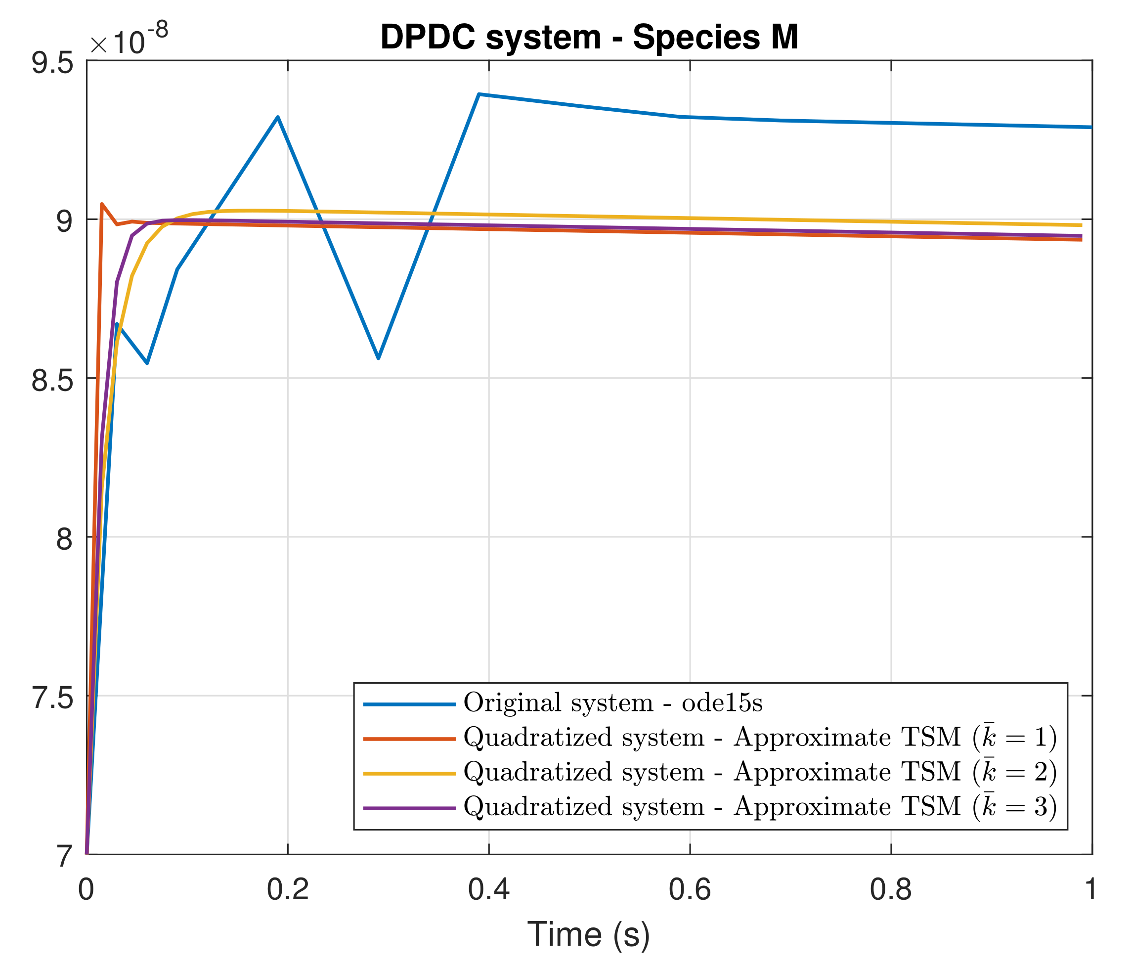
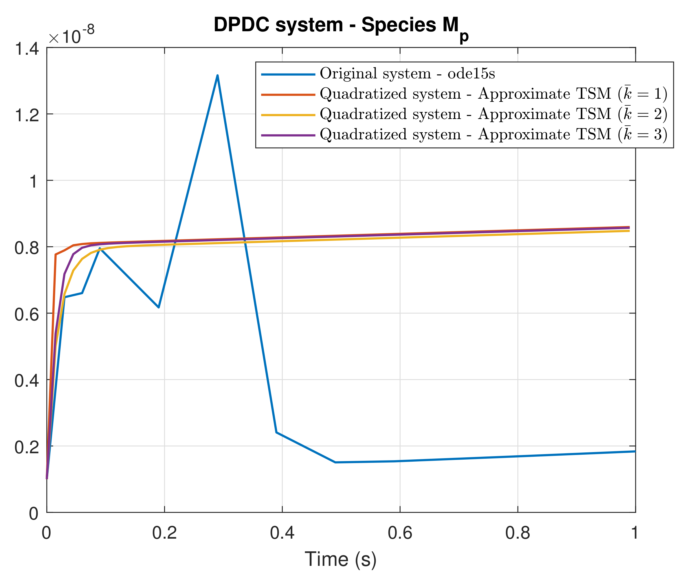
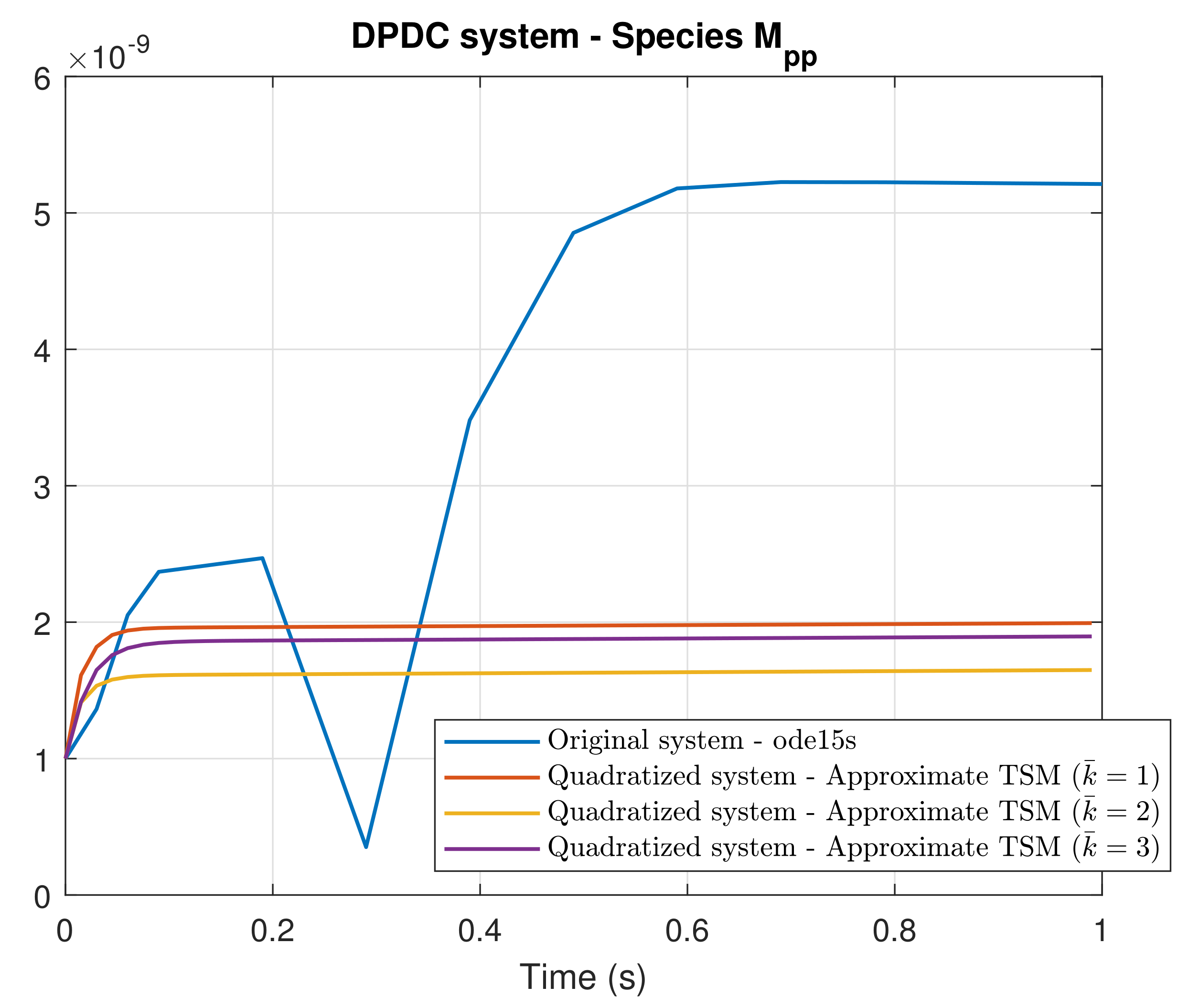
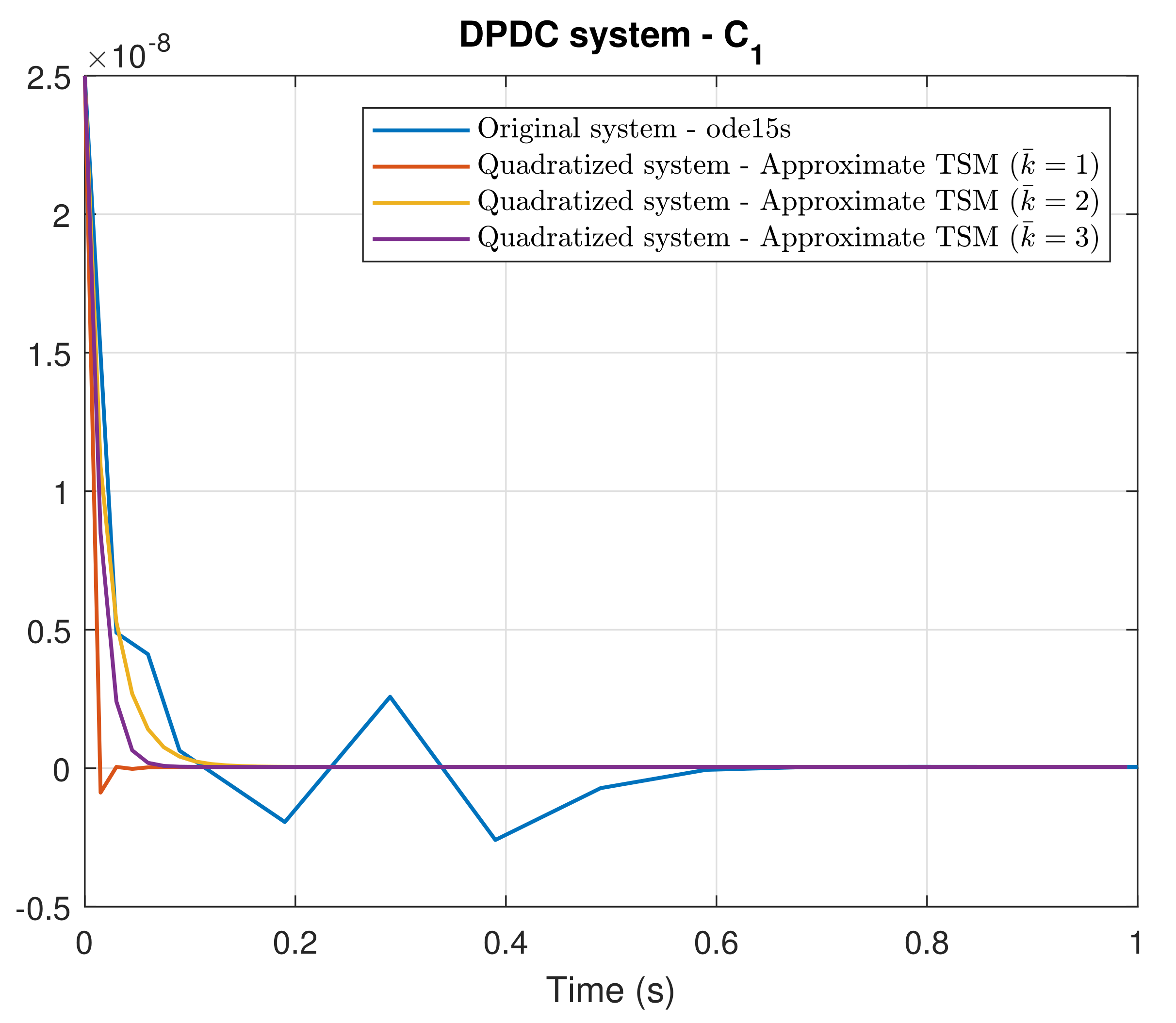
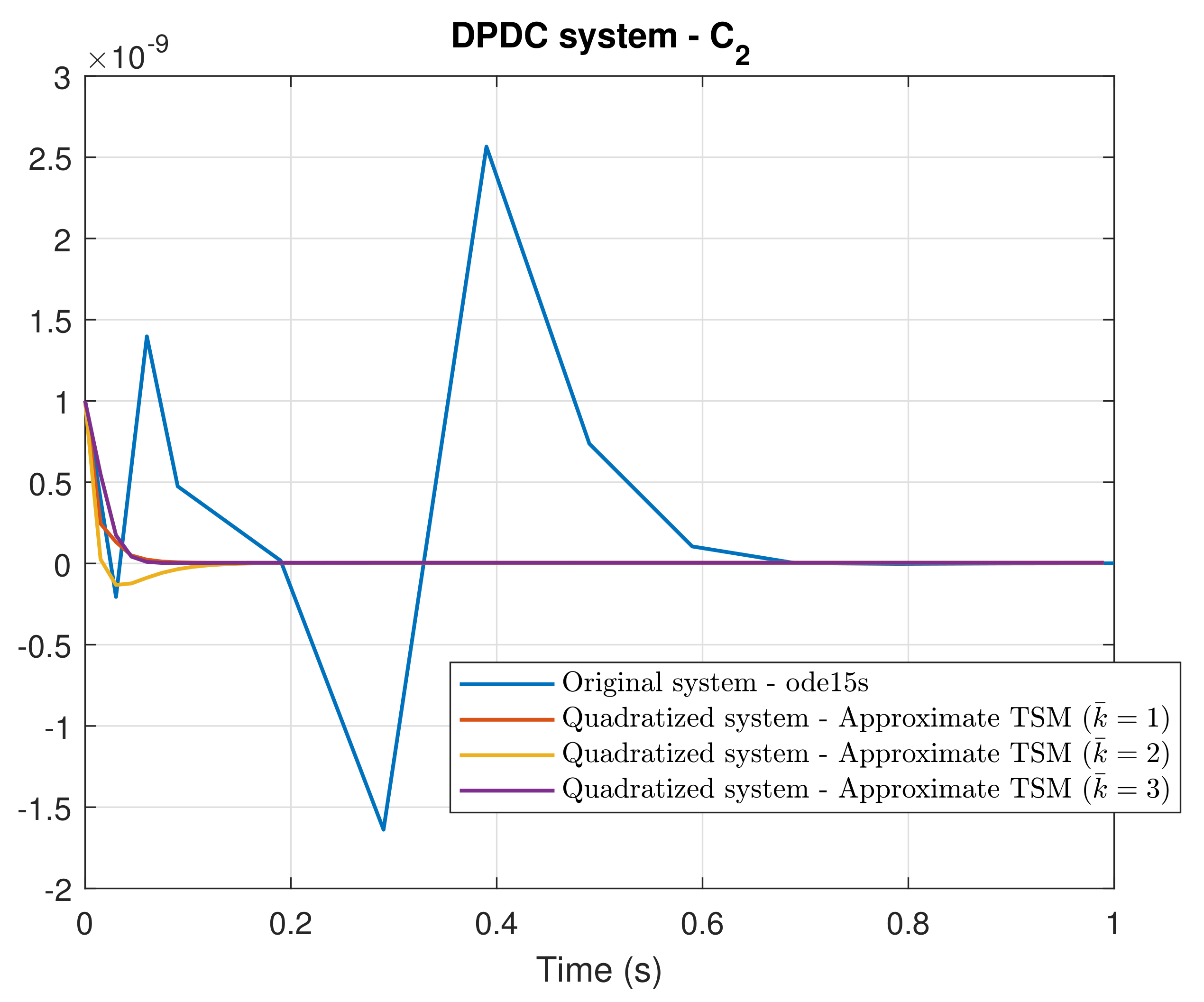
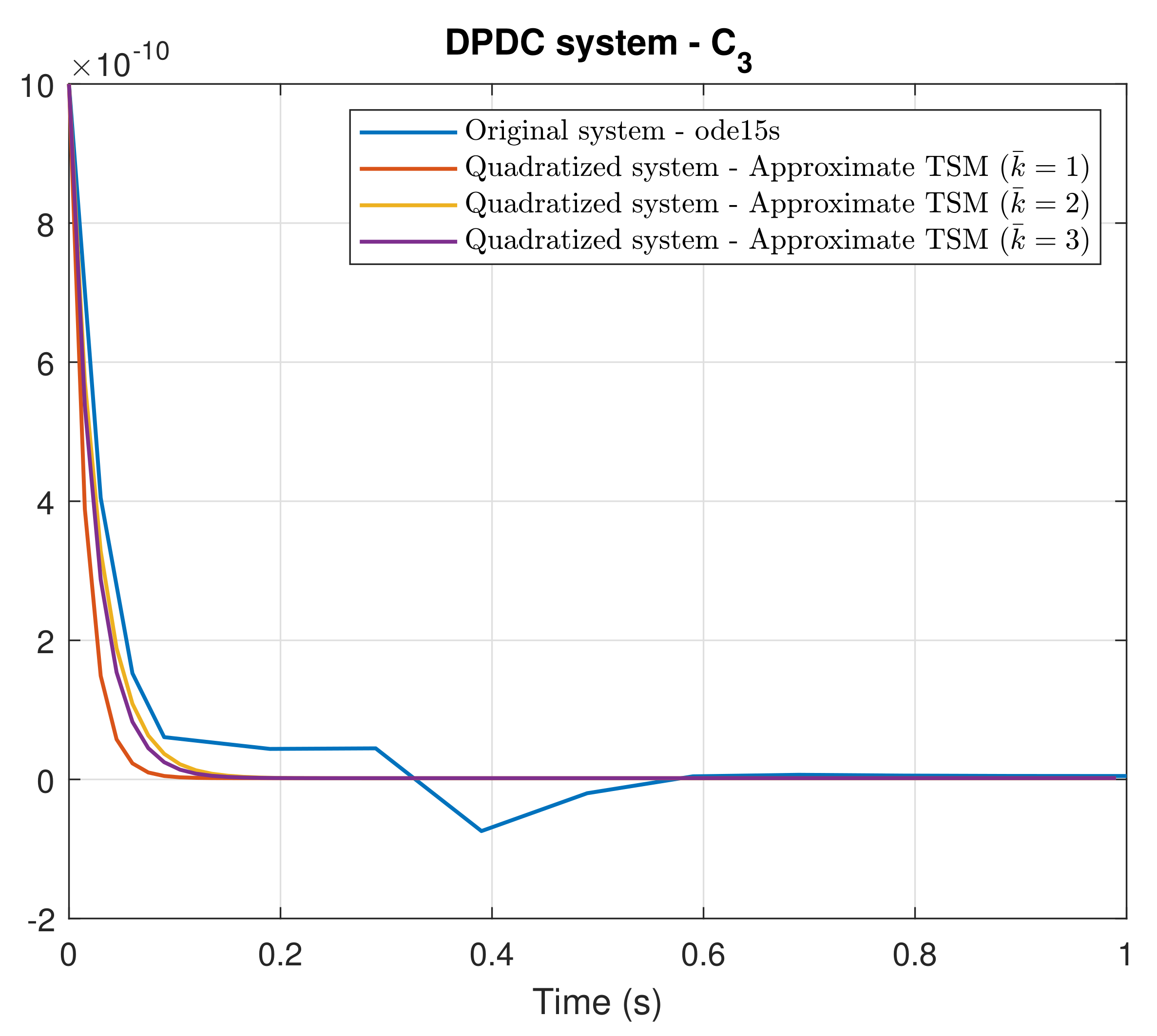
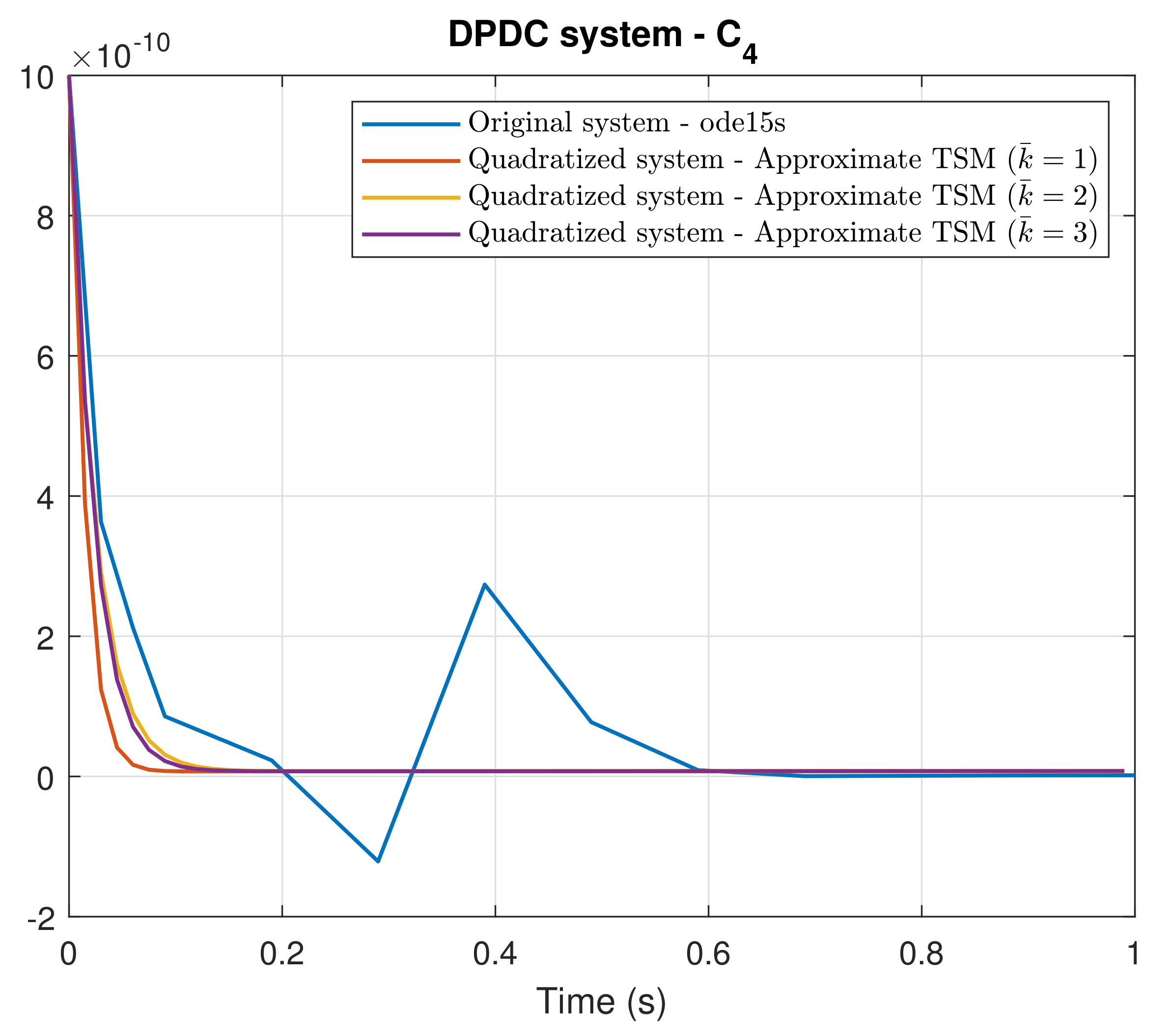
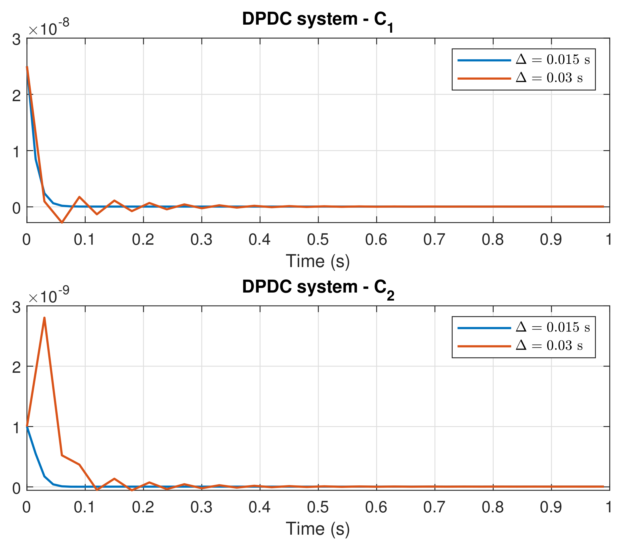
4. Simulation Results

Numerical simulations of the system (16), quadratized in the form (8) as developed in the previous section, have been performed in the Matlab® suite. Inspired by the parameter choices in [14,17], we consider the following parameters:
k j 1 = 4 · 10 8 M 1 s 1 , k j 1 = 25 s 1 , k j 2 = 15 s 1 , j = 1 , 2 , 3 , 4 ,
with total amounts (14) and (15) equal to
M T = k 11 + k 12 k 11 , K T = P T = 10 3 · M T .
We start from the initial conditions (at time t 0 = 0 )
x 1 ( 0 ) = 0.70 M T , x 4 ( 0 ) = 0.25 M T , x i ( 0 ) = 0.01 M T for i = 2 , 3 , 5 , 6 , 7 ,
where the initial states of the adjoint variables x j ( 0 ) , for j = 8 , , 24 , are uniquely determined from (17) and (20). The sampling interval has been set to Δ = 0.015 s and the overall simulation time is 1 s. For the given choice of parameters and initial conditions, simulations performed according to the standard ODE45 Matlab® solver, based on the Dormand–Prince Runge–Kutta method [27] with default settings, are aborted by Matlab for not being able to meet integration tolerances.
Figure 1, Figure 2, Figure 3, Figure 4, Figure 5, Figure 6 and Figure 7 show the numerical solution obtained for variables x 1 , , x 7 by means of the ODE15s Matlab® variable-order solver for stiff differential equations [28] compared with the method of quadratization and truncated TSM integration proposed in this paper. It is clearly observed that the substrate trajectories provided by ode15s oscillate, while our approach provides a smoother behavior. Regards to the complexes, ode15s trajectories become negative, which is qualitatively inconsistent by virtue of Remark 1, as we know that the system (16) is positive. The same occurs with C 1 for the TSM method with truncation order k ¯ = 1 (Euler), see Figure 4, and with C 2 for the TSM method with k ¯ = 2 , see Figure 5. Instead, the TSM method applied to the quadratized system with truncation order k ¯ = 3 exhibits non-negative solutions for all the variables.
Figure 8 shows the trajectories of complexes C 1 (top panel) and C 2 (bottom panel), obtained with sampling time Δ = 0.015 s, compared with the same trajectories computed with a doubled sample interval Δ = 0.03 s, and the same truncation order k ¯ = 3 of the TSM method. It is apparent that the choice of a sufficiently small sampling interval, jointly with a sufficiently high truncation order, is crucial for the numerical stability of the algorithm. In particular, both C 1 and C 2 violate again the non-negativity constraint in the case Δ = 0.03 s, as already observed for Δ = 0.015 s and low truncation orders in Figure 4 and Figure 5, with a notable oscillating behavior and an evident initial overshoot of species C 2 . Note that the pattern of damped oscillations in Figure 4, Figure 6, and Figure 8 is not surprising in numerical simulation and identification in biochemical and biological contexts, for instance, a similar behavior may indeed result from the optimization of the power of the error in multiple linear regression under the assumption of generalized Gauss-Laplace distribution [29].
In summary, the method proposed in this paper seems to be able to return meaningful solutions in the numerical simulation of particular biological conditions when standard solvers may fail.

5. Discussion

In this work, we proposed a novel approach to the problem of integrating the solution of biological systems expressed by stiff differential equations (for example, those exhibiting an apparent double time-scale separation). To overcome typical numerical issues related to the numerical integration of this kind of system by means of existing solvers, we here rely on recent work exploiting the so-called quadratization of ODEs, which allows embedding the original dynamics in a higher-dimensional space where the system is quadratic and differentiation formulae of any order are computable by means of simple recursions. Such derivatives are exploited within a truncated Taylor Series expansion to build an approximate simple integration scheme, which is proved to work accurately in the in silico simulation of the Double Phoshphorylation/Dephoshphorylation Cycle (DPDC), which is an important regulatory mechanism present in cells. Ongoing and future work is focusing on the construction of a numerical scheme that might overcome the curse of dimensionality due to the computation of coefficients of the high-order terms in the Taylor series expansion for the augmented quadratized dynamics.

Author Contributions

Conceptualization, investigation, writing—review and editing, resources, A.B., F.C. and P.P.; writing—original draft preparation, formal analysis, A.B. and P.P.; methodology, F.C.; software, A.B.; supervision, P.P. All authors have read and agreed to the published version of the manuscript.

Funding

This research received no external funding.

Institutional Review Board Statement

Not applicable.

Informed Consent Statement

Not applicable.

Data Availability Statement

Not applicable.

Conflicts of Interest

The authors declare no conflict of interest.

References

  1. Cooper, G. The Cell, a Molecular Approach; Sinauer Associates: Sunderland, MA, USA, 2000. [Google Scholar]
  2. Chang, R. Physical Chemistry for the Chemical and Biological Sciences; University Science Books: New York, NY, USA, 2000. [Google Scholar]
  3. Nash, P.; Tang, X.; Orlicky, S.; Chen, Q.; Gertler, F.B.; Mendenhall, M.D.; Sicheri, F.; Pawson, T.; Tyers, M. Multisite phosphorylation of a CDK inhibitor sets a threshold for the onset of DNA replication. Nature 2001, 414, 514–521. [Google Scholar] [CrossRef]
  4. Palumbo, P.; Vanoni, M.; Cusimano, V.; Busti, S.; Marano, F.; Manes, C.; Alberghina, L. Whi5 phosphorylation embedded in the G1/S network dynamically controls critical cell size and cell fate. Nat. Commun. 2016, 7, 11372. [Google Scholar] [CrossRef] [Green Version]
  5. Ionescu, A.E.; Mentel, M.; Munteanu, C.V.A.; Sima, L.E.; Martin, E.C.; Necula-Petrareanu, G.; Szedlacsek, S.E. Analysis of EYA3 Phosphorylation by Src Kinase Identifies Residues Involved in Cell Proliferation. Int. J. Mol. Sci. 2019, 20, 6307. [Google Scholar] [CrossRef] [Green Version]
  6. Salazar, C.; Höfer, T. Multisite protein phosphorylation—From molecular mechanisms to kinetic models. FEBS J. 2009, 276, 3177–3198. [Google Scholar] [CrossRef]
  7. Salazar, C.; Brümmer, A.; Alberghina, L.; Höfer, T. Timing control in regulatory networks by multisite protein modifications. Trends Cell Biol. 2010, 20, 634–641. [Google Scholar] [CrossRef] [PubMed]
  8. Ortega, F.; Garcés, J.L.; Mas, F.; Kholodenko, B.N.; Cascante, M. Bistability from double phosphorylation in signal transduction. FEBS J. 2006, 273, 3915–3926. [Google Scholar] [CrossRef]
  9. Bersani, A.M.; Borri, A.; Carravetta, F.; Mavelli, G.; Palumbo, P. On a stochastic approach to model the double phosphorylation/dephosphorylation cycle. Math. Mech. Complex Syst. 2020, 8, 261–285. [Google Scholar] [CrossRef]
  10. Ramesh, V.; Krishnan, J. Symmetry breaking meets multisite modification. Elife 2021, 10, e65358. [Google Scholar] [CrossRef] [PubMed]
  11. Bersani, A.M.; Bersani, E.; Dell’Acqua, G.; Pedersen, M.G. New trends and perspectives in nonlinear intracellular dynamics: One century from Michaelis–Menten paper. Contin. Mech. Termodyn. 2015, 27, 659–684. [Google Scholar] [CrossRef]
  12. Cornish-Bowden, A. One hundred years of Michaelis-Menten kinetics. Perspect. Sci. 2015, 4, 3–9. [Google Scholar] [CrossRef]
  13. Michaelis, L.; Menten, M. Kinetics of invertase action. Biochem. Z. 1913, 49, 333–369. [Google Scholar]
  14. Segel, L. On the validity of the steady state assumption of enzyme kinetics. Bull. Math. Biol. 1988, 50, 579–593. [Google Scholar] [CrossRef]
  15. Barrio, R.; Martínez, M.A.; Pérez, L.; Pueyo, E. Bifurcations and Slow-Fast Analysis in a Cardiac Cell Model for Investigation of Early Afterdepolarizations. Mathematics 2020, 8, 880. [Google Scholar] [CrossRef]
  16. Mohd Ijam, H.; Ibrahim, Z.B. Diagonally Implicit Block Backward Differentiation Formula with Optimal Stability Properties for Stiff Ordinary Differential Equations. Symmetry 2019, 11, 1342. [Google Scholar] [CrossRef] [Green Version]
  17. Borri, A.; Carravetta, F.; Palumbo, P. Time series expansion to find solutions of nonlinear systems: An application to enzymatic reactions. In Proceedings of the 2020 European Control Conference (ECC), St. Petersburg, Russia, 12–15 May 2020; pp. 749–754. [Google Scholar]
  18. Bersani, A.M.; Dell’Acqua, G.; Tomassetti, G. On stationary states in the double phosphorylation-dephosphorylation cycle. In Proceedings of the AIP Conference Proceedings, College Park, MD, USA, 28–31 July 2011; American Institute of Physics: College Park, MD, USA, 2011; Volume 1389. [Google Scholar]
  19. Barton, D.; Willers, I.M.; Zahar, R.V.M. Taylor Series Methods for Ordinary Differential Equations—An Evaluation. In Mathematical Software; Rice, J.R., Ed.; Academic Press: New York, NY, USA, 1972; pp. 369–389. [Google Scholar]
  20. Corliss, F.; Chang, Y.F. Solving ordinary differential equations using Taylor Series. ACM Trans. Math. Softw. 1994, 8, 209–233. [Google Scholar] [CrossRef]
  21. Corliss, G.F.; Kirlinger, G. On implicit Taylor series method for stiff ODEs. In Proceedings of the SCAN 91: International Symposium on Computer Arithmetic and Scientific Computing, Oldenburg, Germany, 1–4 October 1991. [Google Scholar]
  22. Barton, D. On Taylor series and stiff equations. ACM Trans. Math. Softw. 1980, 6, 280–294. [Google Scholar] [CrossRef]
  23. Barrio, R. Sensitivity analysis of ODEs/DAEs using the Taylor series method. SIAM J. Sci. Comput. 2006, 6, 1929–1947. [Google Scholar] [CrossRef]
  24. Carravetta, F. Global Exact Quadratization of Continuous-Time Nonlinear Control Systems. SIAM J. Control Optim. 2015, 53, 235–261. [Google Scholar] [CrossRef]
  25. Carravetta, F. On the Solution Calculation of Nonlinear Ordinary Differential Equations via Exact Quadratization. J. Differ. Equ. 2020, 269, 11328–11365. [Google Scholar] [CrossRef]
  26. Farina, L.; Rinaldi, S. Positive Linear Systems: Theory and Applications; John Wiley & Sons: Hoboken, NJ, USA, 2000. [Google Scholar]
  27. Dormand, J.R.; Prince, P.J. A family of embedded Runge-Kutta formulae. J. Comput. Appl. Math. 1980, 6, 19–26. [Google Scholar] [CrossRef] [Green Version]
  28. Shampine, L.F.; Reichelt, M.W. The MATLAB ODE Suite. SIAM J. Sci. Comput. 1997, 18, 1–22. [Google Scholar] [CrossRef] [Green Version]
  29. Jäntschi, L.; Bálint, D.; Bolboacă, S.D. Multiple Linear Regressions by Maximizing the Likelihood under Assumption of Generalized Gauss-Laplace Distribution of the Error. Comput. Math. Methods Med. 2016, 2016, 8578156. [Google Scholar] [CrossRef] [PubMed]
Figure 1. Trajectory of species M via quadratization of Equation (16) and approximate TSM method compared with the Matlab® ODE15s solution. The maximum truncation order has been set to k ¯ = 3 .
Symmetry 13 01684 g001
Figure 2. Trajectory of species M p via quadratization of Equation (16) and approximate TSM method compared with the Matlab® ODE15s solution. The maximum truncation order has been set to k ¯ = 3 .
Symmetry 13 01684 g002
Figure 3. Trajectory of species M p p via quadratization of Equation (16) and approximate TSM method compared with the Matlab® ODE15s solution. The maximum truncation order has been set to k ¯ = 3 .
Symmetry 13 01684 g003
Figure 4. Trajectory of species C 1 via quadratization of Equation (16) and approximate TSM method compared with the Matlab® ODE15s solution. The maximum truncation order has been set to k ¯ = 3 .
Symmetry 13 01684 g004
Figure 5. Trajectory of species C 2 via quadratization of Equation (16) and approximate TSM method compared with the Matlab® ODE15s solution. The maximum truncation order has been set to k ¯ = 3 .
Symmetry 13 01684 g005
Figure 6. Trajectory of species C 3 via quadratization of Equation (16) and approximate TSM method compared with the Matlab® ODE15s solution. The maximum truncation order has been set to k ¯ = 3 .
Symmetry 13 01684 g006
Figure 7. Trajectory of species C 4 via quadratization of Equation (16) and approximate TSM method compared with the Matlab® ODE15s solution. The maximum truncation order has been set to k ¯ = 3 .
Symmetry 13 01684 g007
Figure 8. Trajectories of species C 1 (top panel) and C 2 (bottom panel) via quadratization of Equation (16) and approximate TSM method, with truncation order set to k ¯ = 3 , for two different values of the sampling interval Δ .
Symmetry 13 01684 g008
Publisher’s Note: MDPI stays neutral with regard to jurisdictional claims in published maps and institutional affiliations.

