Generating the Triangulations of the Torus with the Vertex-Labeled Complete 4-Partite Graph K_2,2,2,2

Abstract

Using the orbit decomposition, a new enumerative polynomial $P\left(x\right)$ is introduced for abstract (simplicial) complexes of a given type, e.g., trees with a fixed number of vertices or triangulations of the torus with a fixed graph. The polynomial has the following three useful properties. (I) The value $P\left(1\right)$ is equal to the total number of unlabeled complexes (of a given type). (II) The value of the derivative $P^{\prime }\left(1\right)$ is equal to the total number of nontrivial automorphisms when counted across all unlabeled complexes. (III) The integral of $P\left(x\right)$ from 0 to 1 is equal to the total number of vertex-labeled complexes, divided by the order of the acting group. The enumerative polynomial $P\left(x\right)$ is demonstrated for trees and then is applied to the triangulations of the torus with the vertex-labeled complete four-partite graph $G=K_{2,2,2,2}$, in which specific case $P\left(x\right)=x^{31}$. The graph G embeds in the torus as a triangulation, $T\left(G\right)$. The automorphism group of G naturally acts on the set of triangulations of the torus with the vertex-labeled graph G. For the first time, by a combination of algebraic and symmetry techniques, all vertex-labeled triangulations of the torus (12 in number) with the graph G are classified intelligently without using computing technology, in a uniform and systematic way. It is helpful to notice that the graph G can be converted to the Cayley graph of the quaternion group $Q_8$ with the three imaginary quaternions i, j, k as generators.

1. Introduction

Graph theory and its applications (polyhedra, enumeration, coloring, fullerenes, etc.) has received increasing attention in recent years [1,2,3,4,5], which has paved the way for more directions of research.

In labeled graph enumeration problems, the vertices of the graph are labeled to be distinguishable from each other, while in unlabeled graph enumeration problems any admissible permutation of the vertices is regarded as producing the same graph, so the vertices are considered unlabeled. In general, labeled problems are usually easier than unlabeled ones. For example, Cayley’s tree formula [6,7] gives the number, $n^{n-2}$, of trees with n vertices bijectively labeled by $1,\dots ,n$, whereas the number of unlabeled trees with n vertices can only be evaluated as the coefficients of a generating function [8,9]. The number $n^{n-2}$ can be interpreted as the number of different ways of placing n given folders on the desktop into the one a priori chosen out of them and fixed (the root folder). The orbit decomposition [10] is an important tool for reducing unlabeled problems to labeled ones: Each unlabeled class is considered to be a symmetry class, or an isomorphism class, of labeled graphs. In the current paper we introduce a new enumerative polynomial $P\left(x\right)$ which is a bridge between the labeled and unlabeled settings.

A graph consists of a finite set of vertices, some of which are connected by edges. To “embed a graph in a surface” is, loosely speaking, to draw it on that surface without any edges crossing. An embedding of a graph in a surface is called a closed 2-cell embedding if the surface breaks up into a union of connected components, the faces of the embedding, each of which is bounded by a (simple) cycle (without repeated vertices) in the graph. A closed 2-cell embedding of a graph in a surface is called triangular or a triangulation if each face is triangular, i.e., bounded by a cycle of length 3 (that is, consisting of three edges) of the graph embedded. Throughout this paper we assume all graphs to be simple, i.e., without loops or multiple edges.

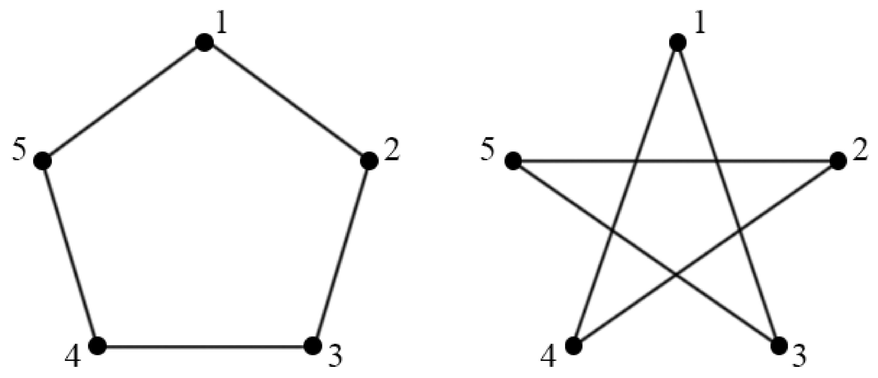
Unlabeled graphs are considered up to isomorphism. For example, all vertex-labeled cycles of length 5 are isomorphic and thus represent the same unlabeled graph, $C_5$, up to isomorphism. The vertices of this graph can be assigned labels 1, 2, 3, 4, 5 in twelve different ways. Furthermore, the 12 different vertex-labeled graphs split into six pairs of graphs which are the complementarities of each other (in each pair); one such pair is shown in Figure 1. (See Remark 1 at the end of Section 6).

Graphs can be thought of as simplicial 1-complexes (that is, 1-dimensional complexes) while triangulations of surfaces can be thought of as simplicial 2-complexes. In general, a simplicial complex $\mathcal{K}$ is a collection of simplices which satisfies the following conditions: Every face of a simplex of $\mathcal{K}$ is a simplex of $\mathcal{K}$, and the intersection of any two simplices in $\mathcal{K}$ is either empty or is a face of both. A simplicial d-complex is a simplicial complex in which the largest dimension of any simplex is d. Combinatorics studies abstract simplicial complexes, while geometry studies geometric simplicial complexes.

Two unlabeled triangulations are called isomorphic provided there is a bijection between their vertex sets, which sends edges to edges and faces to faces. Two triangulations with the same vertex-labeled graph are considered different provided one has a face determined by some three vertices with specific labels while the other does not. Section 6 presents pairs of different triangulations of the torus with the complete vertex-labeled 4-partite graph $G=K_{2,2,2,2}$. 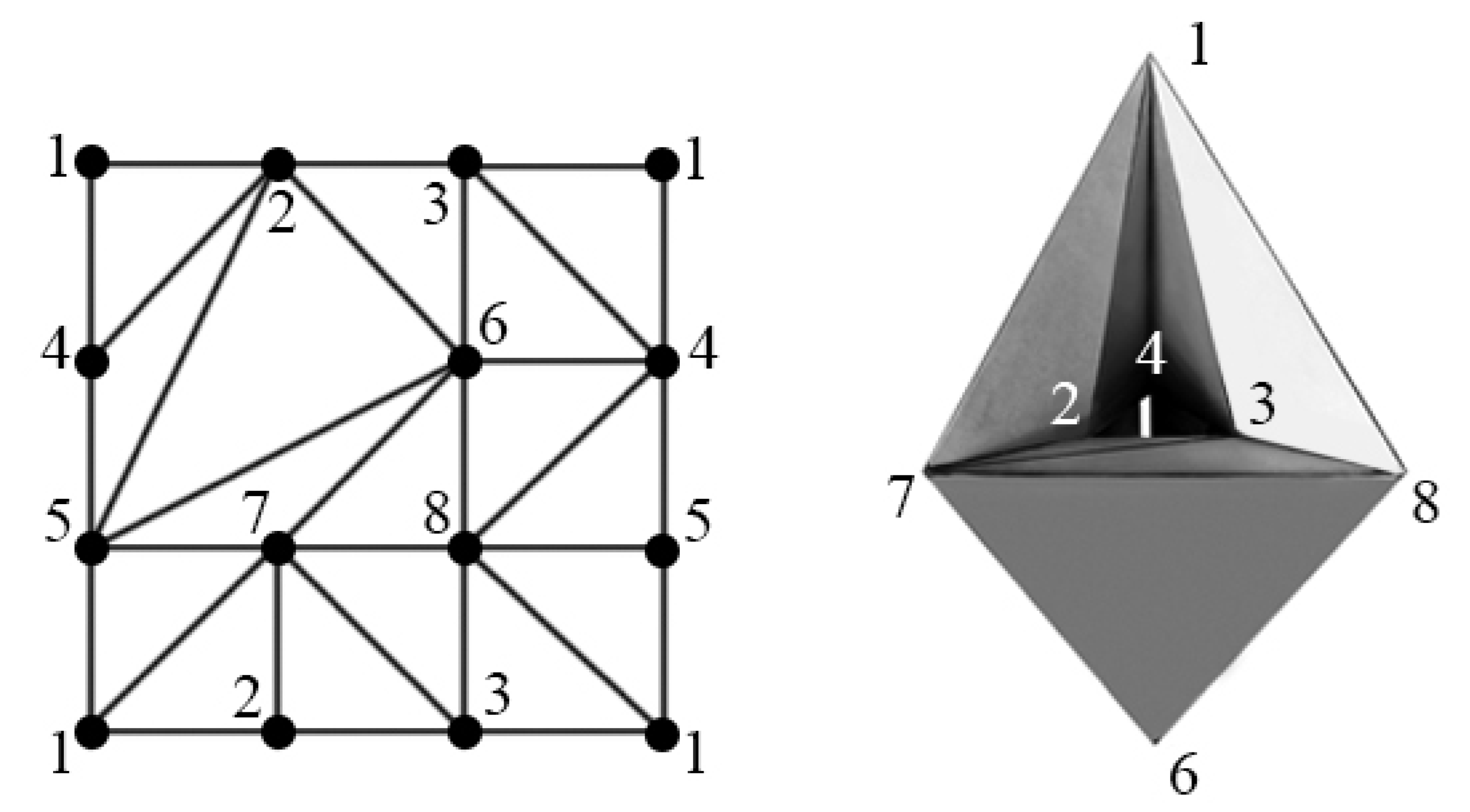Moreover, some of the pairs have no (2-)faces in common at all (just like the complementary graphs in Figure 1 have no 1-faces (edges) in common); triangulations in such pairs are complementary of each other as labeled simplicial 2-complexes. On the other hand, such pairs of triangulations represent the same unlabeled triangulation, the 8-vertex 6-regular triangulation $T\left(G\right)$ of the torus which is known [11,12] to be a unique (up to isomorphism) triangular embedding of the graph $G=K_{2,2,2,2}$ in the torus (see Figure 2, left, identify the sides of the rectangle, in pairs, to obtain a torus). The complete graph $K_8$ has all 28 edges connecting its 8 vertices; the 8-vertex graph $K_{2,2,2,2}$ is in fact the complete graph $K_8$ with four independent edges deleted. In Section 5 and Section 6, we use the same notations, G and $T\left(G\right)$, in both labeled and unlabeled settings; for example, in the unlabeled setting, the triangulation $T\left(G\right)$ means the one in Figure 2 (left) with the labels removed.

The 16-cell, or the 4-dimensional regular cross-polytope, is bounded by 16 three-dimensional facets (a.k.a. 3-faces or 3-cells), each of which is a regular tetrahedron. The 16-cell has 8 vertices, 24 edges, and 32 triangular (2-)faces. The following are the eight vertices of the 16-cell: $(\pm 1,0,0,0)$, $(0,\pm 1,0,0)$, $(0,0,\pm 1,0)$, $(0,0,0,\pm 1)$. All the vertices are connected by edges except opposite pairs. The 16-cell is one of the six regular convex 4-polytopes (a.k.a. polychora). The importance and significance of the graph $G=K_{2,2,2,2}$ are justified by the fact that G is the 1-skeleton (graph) of the 16-cell.

The results of the current paper are primarily concerned with the symmetry relations of the graph $G=K_{2,2,2,2}$ and the triangulation $T\left(G\right)$ of the torus with this graph G (Figure 2, left). Additionally, the triangulation $T\left(G\right)$ is known [11,12] as one of the 21 so-called irreducible triangulations of the torus. Furthermore, $T\left(G\right)$ can be realized geometrically [13] as a toroidal polyhedral suspension in 3-dimensional space ${\mathbb{R}}^3$, as shown in Figure 2 (right), and as a 2-dimensional noble polyhedron in 4-dimensional space ${\mathbb{R}}^4$, i.e., a polyhedron which is isohedral (all faces are similar) and isogonal (all vertices are similar), whose properties are studied extensively in [2].

As the main result of the current paper, it is shown ( Theorem 2, Section 6) how to generate all different triangulations of the torus, totaling 12 in number, with the vertex-labeled graph $G=K_{2,2,2,2}$ in an intelligent fashion without using computer resources. Although explicit identification of the 12 triangulations was done [14] a long time ago in 1987 by a direct exhaustive computer search (Fortran was used as a general-purpose programming language in those earlier years), the structure of the set of the 12 triangulations remained unclear up to now. The structure and a related classification of the 12 triangulations are revealed in Theorem 2 in algebraic terms of certain quotient group action. The importance of the classification obtained is seen in the geometric realization: Geometrically, the 12 vertex-labeled triangulations correspond to different (as point-sets) 2-dimensional toroidal subcomplexes of the 16-cell in ${\mathbb{R}}^4$. Therefore, as a byproduct, we obtain all two-dimensional tori in the 2-skeleton of the 16-cell; their realization in a Schlegel diagram of the 16-cell would lead to new toroidal polyhedra in ${\mathbb{R}}^3$ (a Schlegel diagram is a projection of the polytope from ${\mathbb{R}}^4$ into ${\mathbb{R}}^3$ through a point just outside one of its facets).

2. Preliminary: The Orbit Decomposition

This section serves as a continuation of the Introduction. The objective is to address key algebraic concepts and known results, presented in Lang’s book [10]. In particular, orbit-stabilizer theory is briefly addressed. The reader will find specific illustration examples in Section 4.

In the general case, let $\mathsf{\Omega }$ be a fixed finite set of unlabeled discrete substructures of some ambient structure. For the sake of certainty, the set $\mathsf{\Omega }$, $={\mathsf{\Omega }}^n$, can be thought of as a set of spanning unlabeled (that is, considered up to isomorphism) subcomplexes of some ambient n-vertex unlabeled simplicial complex ${\mathbb{K}}^d$ with dimension d. Let $\mathcal{K}$ be a spanning simplicial subcomplex of ${\mathbb{K}}^d$. An automorphism of $\mathcal{K}$ is any permutation of the vertex set of ${\mathbb{K}}^d$ which sends m-faces of $\mathcal{K}$ onto m-faces of $\mathcal{K}$, for any m ($0⩽m⩽d$). Let ${\mathsf{\Omega }}_k^n$ be the set of unlabeled n-vertex k-symmetric simplicial subcomplexes of ${\mathbb{K}}^d$, where the term “k-symmetric” means that the automorphism group of the subcomplex has order k. Thus,

$$|{\mathsf{\Omega }}^n|=\sum _k\left|{\mathsf{\Omega }}_k^n\right|.$$

In this paper, the two main instances of ${\mathsf{\Omega }}^n$ are as follows:

(i)

the set of n-vertex trees (Section 4) and

(ii)

the set of triangulations of the torus with the 8-vertex graph $G=K_{2,2,2,2}$ (Section 5 and Section 6).

Let ${\mathsf{\Lambda }}^n$ be the set obtained from the set ${\mathsf{\Omega }}^n$ by labeling the n vertices of each element $\mathcal{K}$ of ${\mathsf{\Omega }}^n$ with labels $1,\dots ,n$ bijectively, in all combinatorially different ways. As matter of notation, when $\mathcal{K}$ is assumed to be unlabeled, we write $\mathcal{K}\in {\mathsf{\Omega }}^n$, while when $\mathcal{K}$ is understood to be vertex-labeled, we write $\mathcal{K}\in {\mathsf{\Lambda }}^n$. 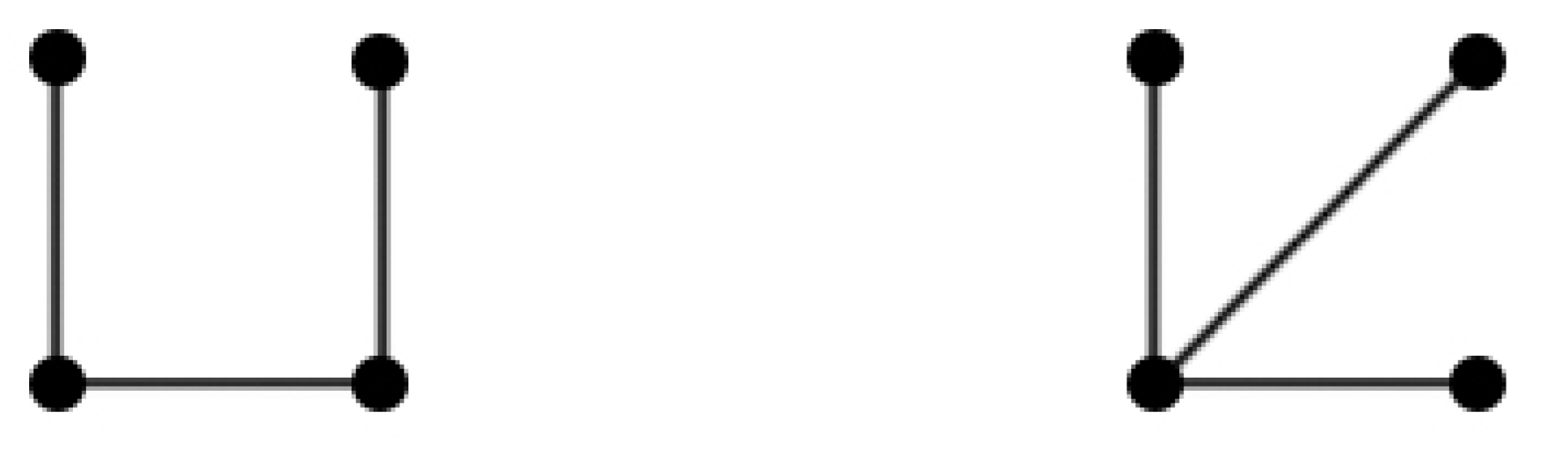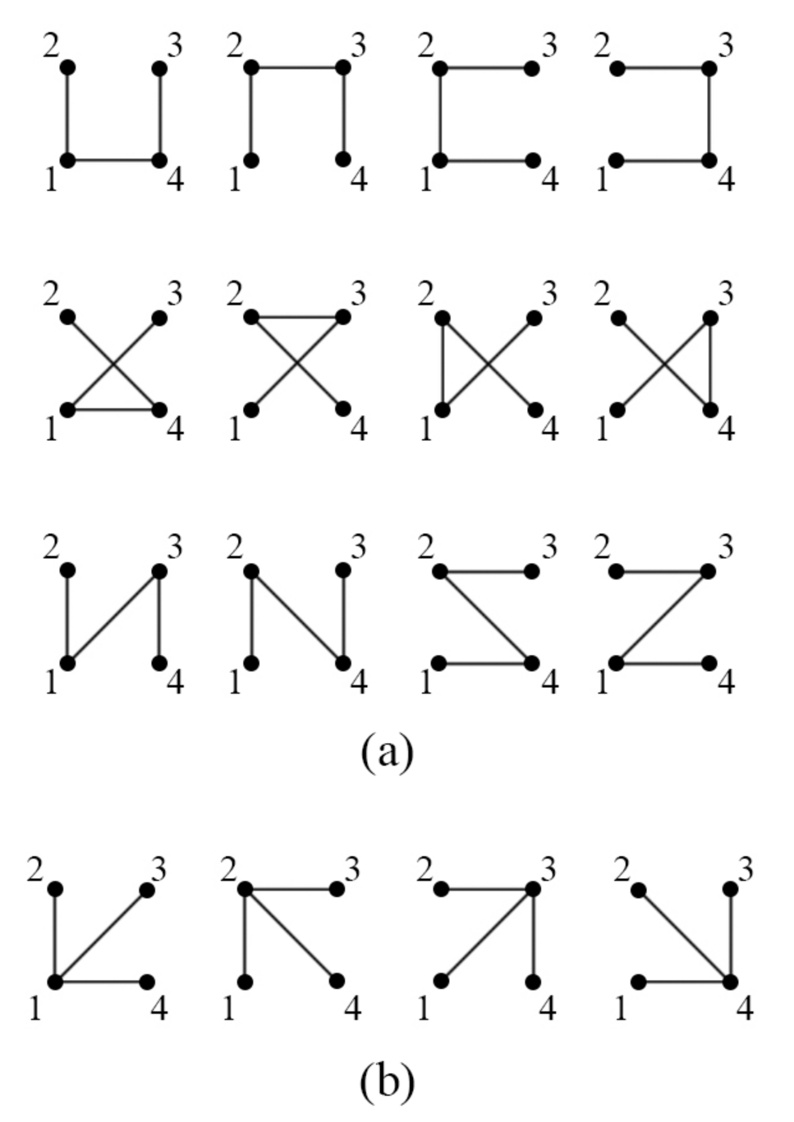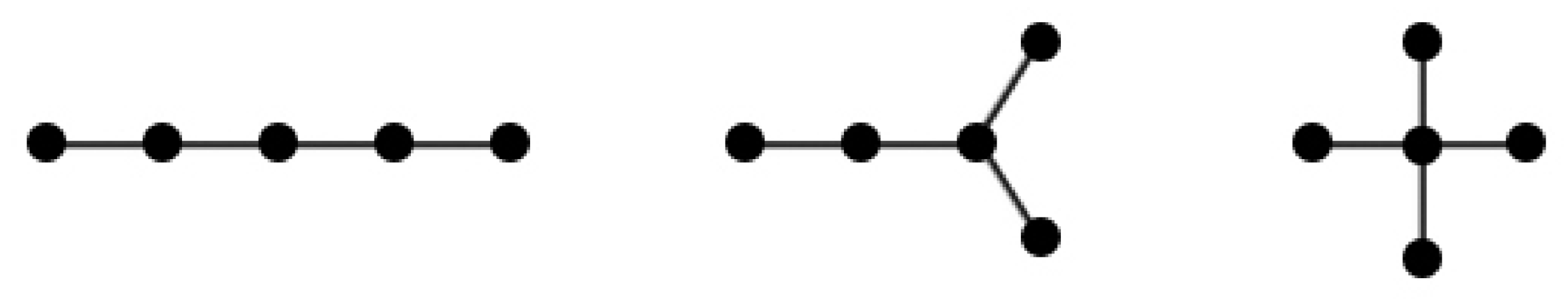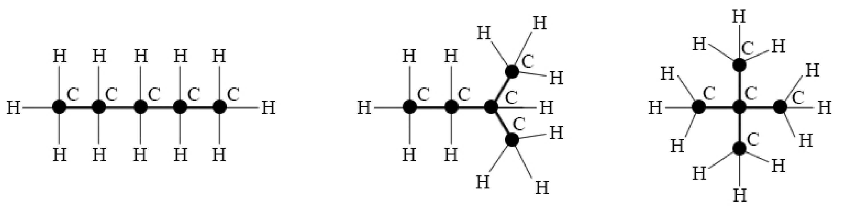Two vertex-labeled simplicial complexes ${\mathcal{K}}_1$, ${\mathcal{K}}_2\in {\mathsf{\Lambda }}^n$ are considered different provided there is a facet of ${\mathcal{K}}_1$ with vertices with certain labels but there is no facet of ${\mathcal{K}}_2$ with the same set of labels. For example, all pairwise different vertex labelings of a 4-vertex path of length 3 with labels $1,2,3,4$ will be shown in Section 4.1

Let $\mathsf{\Gamma }=\mathrm{Aut}\left({\mathbb{K}}^d\right)$ be the automorphism group of the ambient simplicial complex ${\mathbb{K}}^d$ with n vertices. Thus, $\mathsf{\Gamma }$ is a subgroup of the symmetric group $S_n$ (that is, the group which consists of all $n!$ permutations of the n-element set $\{1,2,\dots ,n\}$) and acts (left) on the set ${\mathsf{\Lambda }}^n$: Under this group action, the effect of $\gamma$ ($\gamma \in \mathsf{\Gamma }$) on $\mathcal{K}$ ($\mathcal{K}\in {\mathsf{\Lambda }}^n$) is the new vertex labeling of $\mathcal{K}$, denoted by $\gamma ·\mathcal{K}$, which is obtained from the original one by simply replacing each vertex label u of $\mathcal{K}$ with label $\gamma \left(u\right)$, i.e., the label of the image of the vertex u, under the permutation $\gamma$, in $\mathcal{K}$.

Let $\mathcal{K}$ be an element of ${\mathsf{\Lambda }}^n$. The orbit of $\mathcal{K}$ is the set $\{\gamma ·\mathcal{K}|\gamma \in \mathsf{\Gamma }\}$ of elements in ${\mathsf{\Lambda }}^n$ to which $\mathcal{K}$ can be moved by the elements of $\mathsf{\Gamma }$. This action decomposes the set ${\mathsf{\Lambda }}^n$ into several disjoint orbits. The stabilizer subgroup of $\mathcal{K}$ is defined to be $\{\gamma \in \mathsf{\Gamma }|\gamma ·\mathcal{K}=\mathcal{K}\}$. It is clear that under the action of $\mathsf{\Gamma }$ on ${\mathsf{\Lambda }}^n$ the following three claims hold for any $\mathcal{K}\in {\mathsf{\Lambda }}^n$.

Claim A: The stabilizer subgroup of $\mathcal{K}$ is identical with the automorphism group $\mathrm{Aut}\left(K\right)$.

Claim B: The size of the orbit of $\mathcal{K}$ is equal to the number of different vertex labelings of $\mathcal{K}$.

Claim C: The total number of orbits is equal to $|{\mathsf{\Omega }}^n|$.

Let ${\mathsf{\Lambda }}_k^n$ denote the subset of ${\mathsf{\Lambda }}^n$ whose elements are k-symmetric (as unlabeled simplicial complexes, i.e., with the labels removed). Please note that by Lagrange’s theorem, k is necessarily a divisor of $\left|\mathsf{\Gamma }\right|$. Let $\mathcal{K}\in {\mathsf{\Lambda }}_k^n$. By the Orbit-Stabilizer Theorem [10], the size of the orbit of $\mathcal{K}$ is equal to the index$\left|\mathsf{\Gamma }\right|/k$ of the stabilizer subgroup of $\mathcal{K}$ in the group $\mathsf{\Gamma }$. By Claim C, summing over the $|{\mathsf{\Omega }}_k^n|$ different orbits of k-symmetric elements in ${\mathsf{\Lambda }}_k^n$ gives the following equation:

$$|{\mathsf{\Lambda }}_k^n|=\frac{\left|\mathsf{\Gamma }\right|}{k}\left|{\mathsf{\Omega }}_k^n\right|.$$

(1)

Summing Equation (1) over k gives the following equation:

$$\sum _{k||\mathsf{\Gamma }|}|{\mathsf{\Lambda }}_k^n|=\sum _{k\left|\right|\mathsf{\Gamma }|}\frac{\left|\mathsf{\Gamma }\right|}{k}\left|{\mathsf{\Omega }}_k^n\right|.$$

(2)

Thus, we come to the orbit decomposition formula [10] for the action of the group $\mathsf{\Gamma }$ on the set ${\mathsf{\Lambda }}^n$:

$$|{\mathsf{\Lambda }}^n|=\sum _{i=1}^{|{\mathsf{\Omega }}^n|}\frac{\left|\mathsf{\Gamma }\right|}{\left|\mathrm{Aut}\right({\mathcal{K}}_i\left)\right|},$$

where $\mathrm{Aut}\left({\mathcal{K}}_i\right)$ stands for the automorphism group of any representative element ${\mathcal{K}}_i$ in orbit i.

When it is clear what value n is meant to be, the notations ${\mathsf{\Omega }}_k^n$ and ${\mathsf{\Lambda }}_k^n$ may be abbreviated to ${\mathsf{\Omega }}_k$ and ${\mathsf{\Lambda }}_k$, respectively.

3. A New Enumerative Polynomial

For a given set $\mathsf{\Omega }$ ($={\mathsf{\Omega }}^n$), we introduce a new enumerative polynomial, which is defined by

$$P\left(x\right)(=P_n\left(x\right))=\sum _{k\left|\right|\mathsf{\Gamma }|}\left|{\mathsf{\Omega }}_k\right|x^{k-1}.$$

(3)

This enumerative polynomial has derivative and integral which are combinatorially meaningful.

Theorem 1.

The enumerative polynomial defined by Equation (3) has the following three properties:

(I)

$P\left(1\right)=\left|\mathsf{\Omega }\right|$,

(II)

$P^{\prime }\left(1\right)=\tilde{\alpha }$, the total number of nontrivial automorphisms when counted across all elements of Ω,

(III)

$\underset{0}{\overset{1}{\int }}P\left(x\right)dx=\left|\mathsf{\Lambda }\right|/\left|\mathsf{\Gamma }\right|$.

Proof. 

(I)

Evaluate at $x=1$:

$$P\left(1\right)=\sum _k|{\mathsf{\Omega }}_k|=|\mathsf{\Omega }|.$$

(II)

Evaluate the derivative:

$$P^{\prime }\left(x\right)=\sum _{k\left|\right|\mathsf{\Gamma }|}(k-1)\left|{\mathsf{\Omega }}_k\right|x^{k-2},$$

$$P^{\prime }\left(1\right)=\sum _{k\left|\right|\mathsf{\Gamma }|}(k-1)|{\mathsf{\Omega }}_k|=\sum _{k\left|\right|\mathsf{\Gamma }|}k|{\mathsf{\Omega }}_k|-|\mathsf{\Omega }|.$$

Therefore,

$$P^{\prime }\left(1\right)=\tilde{\alpha }=\alpha -\overline{\alpha },$$

where $\alpha$ is the total number of automorphisms, $\overline{\alpha }$ is the total number of trivial automorphisms, and $\tilde{\alpha }$ is the total number of nontrivial automorphisms when counted across all elements of $\mathsf{\Omega }$.

(III)

Evaluate the integral:

$$\underset{0}{\overset{1}{\int }}P\left(x\right)dx=\sum _{k\left|\right|\mathsf{\Gamma }|}\frac{1}{k}\left|{\mathsf{\Omega }}_k\right|.$$

Thus, by Equation (2):

$$\left|\mathsf{\Gamma }\right|\underset{0}{\overset{1}{\int }}P\left(x\right)dx=\sum _{k\left|\right|\mathsf{\Gamma }|}\frac{\left|\mathsf{\Gamma }\right|}{k}|{\mathsf{\Omega }}_k|=\sum _{k\left|\right|\mathsf{\Gamma }|}|{\mathsf{\Lambda }}_k|=|\mathsf{\Lambda }|.$$

Thus,

$$\underset{0}{\overset{1}{\int }}P\left(x\right)dx=\frac{\left|\mathsf{\Lambda }\right|}{\left|\mathsf{\Gamma }\right|}.$$

The proof is complete. □

4. Examples: Trees

The role of this section is to demonstrate the enumerative polynomial in a simple framework of ordinary trees, i.e., connected graphs without cycles, with a given number of vertices. Specifically for trees with n ($n⩾4$) vertices, the ambient simplicial complex ${\mathbb{K}}^1$ is the complete graph $K_n$, the acting group $\mathsf{\Gamma }$ is the symmetric group $S_n$, and the enumerative polynomial is given by

$$P_n\left(x\right)=\sum _{k|n!}\left|{\mathsf{\Omega }}_k\right|x^{k-1}.$$

4.1. Trees with 4 Vertices

Figure 3 shows two non-isomorphic 4-vertex trees, $T_1$ (left) and $T_2$ (right). It is known ([15] Appendix 3, p. 233) that ${\mathsf{\Omega }}^4$$=\{T_1,T_2\}$. The automorphism groups of $T_1$ and $T_2$ are the symmetric groups $S_2$ and $S_3$ with orders 2 and 6, respectively. Thus,

$$P_4\left(x\right)=x^{2-1}+x^{6-1}=x^5+x,P_4\left(1\right)=2,P_4^{\prime }\left(1\right)=6,{\int }_0^1{P}_4\left(x\right)dx=\frac{2}{3}.$$

Thus, by Theorem 1:

$|{\mathsf{\Omega }}_4|=P_4\left(1\right)=2$,

${\tilde{\alpha }}_4=P_4^{\prime }\left(1\right)=6$,

$|{\mathsf{\Lambda }}_4|=\left({\int }_0^1{P}_4\left(x\right)dx\right)·4!=16=4^{4-2}$ (which agrees with Cayley’s formula for the number of vertex-labeled trees).

The 16 labeled trees on 4 vertices are shown in Figure 4a,b. By Equation (2), the more automorphisms a tree has the fewer copies of that tree there are in the ambient graph.

4.2. Trees with 5 Vertices

Figure 5 shows three pairwise non-isomorphic 5-vertex trees, $T_1$ (left), $T_2$ (middle), and $T_3$ (right). It is known ([15] Appendix 3, p. 233) that ${\mathsf{\Omega }}^5$$=\{T_1,T_2,T_3\}$. The automorphism groups of $T_1,T_2,T_3$ are the symmetric groups $S_2,S_2,S_4$ with orders 2, 2, 24, respectively. Thus,

$$P_5\left(x\right)=x^{2-1}+x^{2-1}+x^{24-1}=x^{23}+2x,P_5^{\prime }\left(x\right)=23x^{22}+2,$$

$$P_5\left(1\right)=3,P_5^{\prime }\left(1\right)=25,{\int }_0^1{P}_5\left(x\right)dx=\frac{25}{24}.$$

Thus, by Theorem 1:

$|{\mathsf{\Omega }}_5|=P_5\left(1\right)=3$,

${\tilde{\alpha }}_5=P_5^{\prime }\left(1\right)=25$,

$|{\mathsf{\Lambda }}_5|=\left({\int }_0^1{P}_5\left(x\right)dx\right)·5!=\frac{25}{24}·120=125=5^{5-2}$ (which agrees with Cayley’s formula for the number of vertex-labeled trees).

On the practical side, trees provide models for saturated acyclic hydrocarbons ([16] Chapter 8, p. 533). The number of different chemical isomers sharing the same chemical formula ${\mathrm{C}}_n{\mathrm{H}}_{2n+2}$ is equal to the number of pairwise non-isomorphic trees with n vertices. For $n=5$, all pairwise non-isomorphic trees with 5 vertices are shown in Figure 5, and the corresponding isomers with the formula ${\mathrm{C}}_5{\mathrm{H}}_{12}$ are listed in Figure 6: pentane, isopentane, neopentane (from left to right).

In conclusion of this section, we mention Bernstein’s theorem [17] restricted to the real axis, which states: $|M^{\prime }\left(1\right)|⩽degM\left(x\right)·|M\left(1\right)|$ for any polynomial $M\left(x\right)$. It is tempting to apply this inequality to the enumerative polynomial $P_n\left(x\right)$ along with its derivative and integral, but it only produces simple corollaries. For instance, apply Bernstein’s theorem to the polynomial $M\left(x\right)={\int }_0^x{P}_n\left(t\right)dt$ in the set ${\mathsf{\Omega }}^n$ of pairwise non-isomorphic trees on n unlabeled vertices ($n⩾4$). Since it can be easily seen that the largest order of the automorphism group of an n-vertex tree is $(n-1)!$, it follows that $degM\left(x\right)⩽(n-1)!$ and, by Bernstein’s theorem, $|M^{\prime }\left(1\right)|=P_n\left(1\right)⩽(n-1)!{\int }_0^1{P}_n\left(x\right)dx$. Thus, by Theorem 1 (I), (III), we come to the following inequality: $|{\mathsf{\Omega }}^n|⩽|{\mathsf{\Lambda }}^n|/n$. Now, applying Cayley’s tree formula, $|{\mathsf{\Lambda }}^n|=n^{n-2}$, we come to the following upper bound on the number of trees with n unlabeled vertices: $|{\mathsf{\Omega }}^n|⩽n^{n-3}$.

5. Symmetry Properties of the Graph $\mathit{G}={\mathit{K}}_{\mathbf{2},\mathbf{2},\mathbf{2},\mathbf{2}}$ and Its Triangular Embeddings in the Torus

We refer the interested reader to White’s textbook [18] for the basics of topological graph theory, including automorphism groups of graphs and Cayley graphs.

Throughout this paper, $T\left(G\right)$ stands for the triangulation of the torus shown in Figure 2 (left) and G ($=K_{2,2,2,2}$) stands for its graph, as specified in the Introduction. It is known [11,12] that the triangulation $T\left(G\right)$ is a unique (up to isomorphism) triangulation of the torus whose graph is isomorphic to $K_{2,2,2,2}$, whence all embeddings of G in the torus are isomorphic as triangulations. Thus, the set $\mathsf{\Omega }={\mathsf{\Omega }}^8$ of all non-isomorphic 8-vertex unlabeled triangulations of the torus, with the graph G, consists of a single element: $\mathsf{\Omega }=\left\{T\right(G\left)\right\}$.

The automorphism group $\mathrm{Aut}\left(G\right)$ of the graph G is identical with the automorphism group of its complementary graph $\mathrm{Aut}\left(\overline{G}\right)\equiv \mathrm{Aut}\left(4K_2\right)$, which is identical with the composition (or wreath product) $S_4\left[\mathrm{Aut}\left(K_2\right)\right]=S_4\left[S_2\right]$ and has order $|S_4|·|S_2{|}^4=4!·{(2!)}^4=384$; see ([18] Chapter 3) for details.

Let the group $\mathsf{\Gamma }=\mathrm{Aut}\left(G\right)$ act (left) on the set $\mathsf{\Lambda }={\mathsf{\Lambda }}^8$ of triangulations of the torus with the 8-vertex-labeled graph G; under this action, the effect of an automorphism $\gamma \in \mathrm{Aut}\left(G\right)$ on $T\left(G\right)$ replaces each vertex label u in $T\left(G\right)$ with $\gamma \left(u\right)$. (Geometrically, the ambient simplicial complex ${\mathbb{K}}^2$ may be thought of as the 2-skeleton of the 16-cell in ${\mathbb{R}}^4$ as discussed at the end of the Introduction.) Since $\mathsf{\Omega }=\left\{T\right(G\left)\right\}$, all triangulations of the torus with the vertex-labeled graph G are in a single orbit under the action of $\mathsf{\Gamma }=\mathrm{Aut}\left(G\right)$ on $\mathsf{\Lambda }$. The automorphism group $\mathrm{Aut}\left(T\right(G\left)\right)$ of the triangulation $T\left(G\right)$ is determined in [13,14]. This group can be generated by the involutions ${\mathsf{\tau }}_1=\left(35\right)\left(47\right)$ and ${\mathsf{\tau }}_2=\left(16\right)\left(37\right)\left(45\right)$ together with the cyclic shift ${\mathsf{\tau }}_3=\left(15276384\right)$ (check with Figure 2, left). Thus, $\left|\mathrm{Aut}\right(T\left(G\right)\left)\right|=2\times 2\times 8=32$, whence $\left|\mathsf{\Omega }\right|=|{\mathsf{\Omega }}_{32}^8|=1$. Summarizing, the enumerative polynomial defined by Equation (3) for the set $\mathsf{\Omega }=\left\{T\right(G\left)\right\}$ can be written down as follows:

$$P\left(x\right)=\sum _{k\left|\right|\mathrm{Aut}\left(G\right)|}|{\mathsf{\Omega }}_k^8|x^{k-1}=\left|{\mathsf{\Omega }}_{32}^8\right|x^{31}=x^{31}.$$

Thus, by Theorem 1 (III),

$$\frac{1}{32}={\int }_0^1{x}^{31}dx=\frac{\left|\mathsf{\Lambda }\right|}{\left|\mathrm{Aut}\right(G\left)\right|}=\frac{\left|\mathsf{\Lambda }\right|}{384},$$

whence the number of triangulations of the torus with the vertex-labeled graph G is equal to 12:

$$\left|\mathsf{\Lambda }\right|=\frac{384}{32}=12.$$

(4)

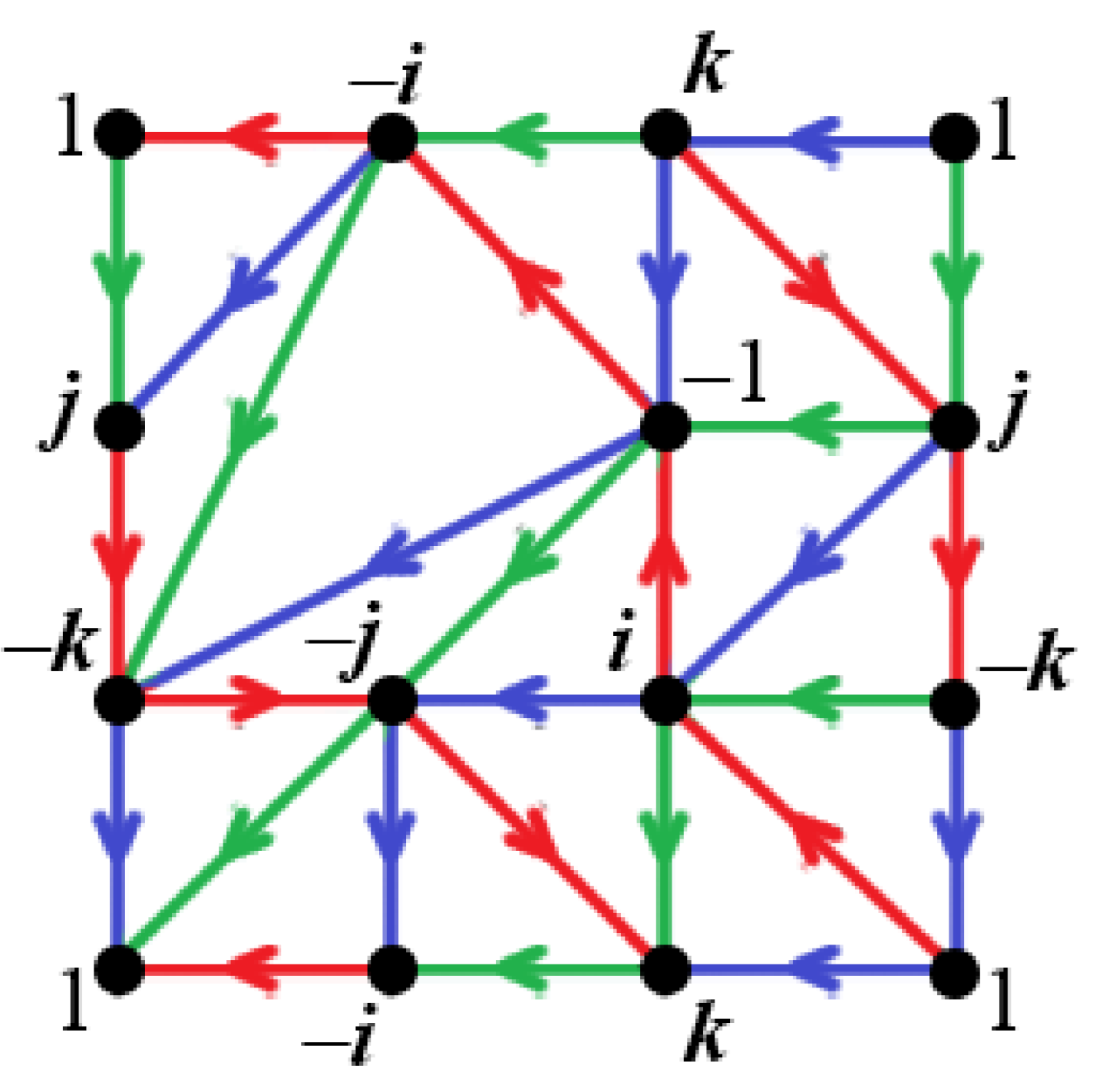
The quaternion group $Q_8$ is a non-abelian group of order 8, isomorphic to the 8-element subset $\{1,i,j,k,-1,-i,-j,-k\}$ of the quaternions under multiplication. The crucial idea is to convert the graph G (Figure 2, left) into the Cayley graph of the quaternion group $Q_8$ by first replacing the labels 1, 2, 3, 4, 5, 6, 7, 8 with the quaternions 1, $-i$, k, j, $-k$, $-1$, $-j$, i (respectively) and then assigning colors and directions to the edges as shown in Figure 7. This conversion will enable us to classify the 12 different triangulations (in Section 6), which number is stated by Equation (4), in a systematic way by a combination of algebraic and symmetry techniques. The red [respectively, green, blue] directed edges correspond to the multiplication by i (on the right) [respectively, by j, k]. The Cayley graph provides the multiplication table of $Q_8$ as a picture in Figure 7; for example, the blue edge directed from j to i in Figure 7 provides the equality $j·k=i$.

It should be noted that the Cayley graph, in fact, depends on the choice of the group generators, and what is often called the Cayley graph of $Q_8$ is the subgraph obtained from Figure 7 by deleting the blue edges. This subgraph corresponds to the set $\{i,j\}$ chosen as a minimal generating set. Furthermore, this subgraph is known [18] to quadrangulate the torus, and it can be thought that the quadrilaterals are dissected into triangles by the blue edges as in Figure 7; the resulting graph triangulates the torus and is called the (extended) Cayley graph of the quaternion group $Q_8$ throughout this paper.

We finally make a useful observation. The edge set of the graph G forms a single orbit under the natural action of the group $\mathsf{\Gamma }\equiv \mathrm{Aut}\left(G\right)$; however, there are two orbits under the action of $\mathrm{Aut}\left(T\right(G\left)\right)$ (as a subgroup of $\mathsf{\Gamma }$). In the latter instance, one orbit has 8 edges and the other one has 16 edges, where the orbit of size 8 coincides with the edge set of the union of two disjoint red cycles (with the directions removed) of length 4 (Figure 7). This can be proved by straightforward inspection of the three generators of $\mathrm{Aut}\left(T\right(G\left)\right)$ as follows: The generator ${\mathsf{\tau }}_1=(j-j)(k-k)$ preserves each of the three colors, while the generators ${\mathsf{\tau }}_2=(1-1)(j-k)(k-j)$ and ${\mathsf{\tau }}_3=(-k-i-j-1kij1)$ preserve the red color, changing green into blue and blue into green (check with Figure 7). Therefore, the representation of the graph G as a triangulation $T\left(G\right)$ of the torus (Figure 2, left) has an advantage before the graph G only as itself: The combinatorial structure of the triangulation $T\left(G\right)$ alone distinguishes the edges that are colored red in Figure 7. (Observe from Figure 7 that the two red cycles are both geodetic and homotopic to each other in the torus; a geodetic cycle C in a graph H is a cycle with the property that for every two vertices $u,v\in C$ at least one of the paths $uCv$ or $vCu$ is a geodesic in H.)

6. Systematic Generation of Triangulations of the Torus with the Vertex-Labeled Graph $\mathit{G}={\mathit{K}}_{\mathbf{2},\mathbf{2},\mathbf{2},\mathbf{2}}$

As we already know by Equation (4), there exist precisely 12 triangular embeddings of the vertex-labeled graph $G=K_{2,2,2,2}$ in the torus. Explicit identification of the 12 triangulations was done in [14] by a direct exhaustive computer search. In this section, it is shown how to generate the 12 triangulations intelligently without using computing technology.

We will use the representation of G in Figure 7 instead of the representation in Figure 2 (left). It should be noted that we regard the Cayley graph in Figure 7 as just replacing the alphabet for labeling the vertices of the original vertex-labeled simple graph G in Figure 2 (left); we will use the same notation for both graphs. The edge colors and directions in Figure 7 will only help us to reveal the structure of the set $\mathsf{\Lambda }$.

Consider the following four permutations of the vertex set of the graph G in Figure 7 (leaving the rest of the vertices fixed):

$$\mathrm{id},{\gamma }_{\mathrm{rot}}=(1i-1-i),$$

$${\gamma }_{\mathrm{ref}}=(1-1),{\gamma }_{\mathrm{rot}}{\gamma }_{\mathrm{ref}}=(1-i)(i-1).$$

It is not hard to verify with Figure 7 that each of the four permutations is an automorphism of the graph G but not each of them is an automorphism of the triangulation $T\left(G\right)$: Although the identity permutation “id” is of course an automorphism of $T\left(G\right)$, none of ${\gamma }_{\mathrm{rot}}$, ${\gamma }_{\mathrm{ref}}$, or ${\gamma }_{\mathrm{rot}}{\gamma }_{\mathrm{ref}}$ is an automorphism of $T\left(G\right)$. 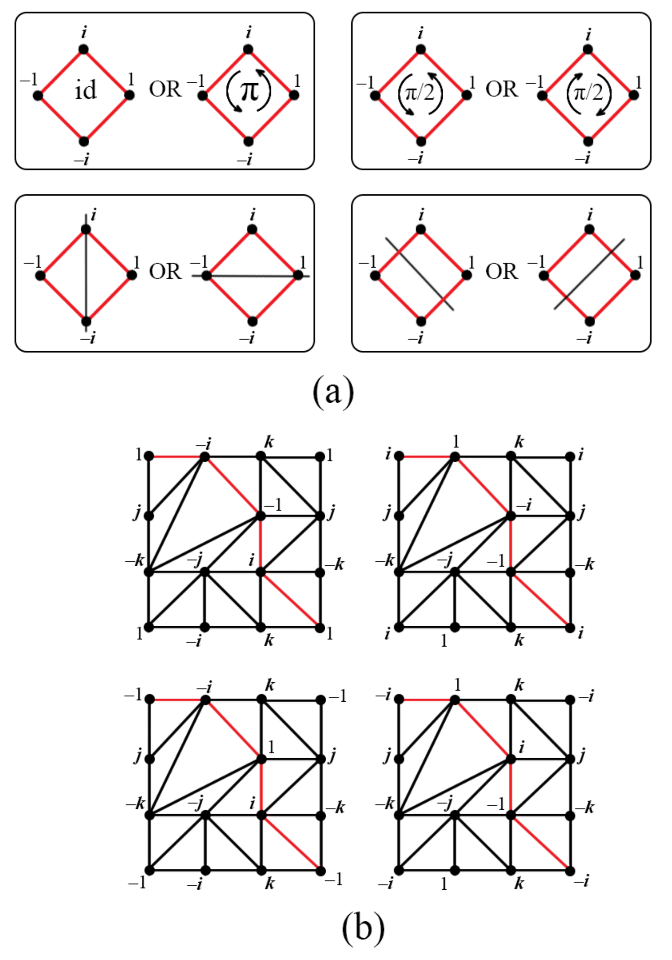The notation is inspired by the observation that the graph automorphism ${\gamma }_{\mathrm{rot}}$ is realized geometrically as a rotation of the square with vertices 1, i, $-1$, $-i$ while the graph automorphisms ${\gamma }_{\mathrm{ref}}$ and ${\gamma }_{\mathrm{rot}}{\gamma }_{\mathrm{ref}}$ are realized geometrically as (axial) reflections of that square as indicated by the self-explanatory pictures in the left-hand sides of the frames of Figure 8a.

For $\gamma \in \mathsf{\Gamma }=\mathrm{Aut}\left(G\right)$, let $\gamma ·T\left(G\right)$ denote the triangulation which is the effect of the permutation $\gamma$ on $T\left(G\right)$ under the action of the group $\mathsf{\Gamma }$ on the set $\mathsf{\Lambda }$ of triangulations of the torus with the vertex-labeled graph G. It is not hard to verify with Figure 7 that the four triangulations $T\left(G\right)$, ${\gamma }_{\mathrm{rot}}·T\left(G\right)$, ${\gamma }_{\mathrm{ref}}·T\left(G\right)$, and ${\gamma }_{\mathrm{rot}}{\gamma }_{\mathrm{ref}}·T\left(G\right)$ (all shown in Figure 8b) are pairwise different. Moreover, the pair of triangulations in each row of Figure 8b have no faces in common at all.

Denote by $D_8=D_8(1,i,-1,-i)$ the dihedral group (often denoted by $D_4$ in geometry) regarded as the automorphism group of the (red) cycle $(1,i,-1,-i)$ of G (with the directions removed). All eight elements of $D_8$ are presented in Figure 8a in the form of a geometric realization. Furthermore, fixing the other four vertices of G (that is, j, $-j$, k, and $-k$), we regard $D_8$ as a subgroup of $\mathsf{\Gamma }=\mathrm{Aut}\left(G\right)$ acting on the set $\mathsf{\Lambda }$. It is not hard to verify that the elements of $D_8$ (graph automorphisms) seen in one frame of Figure 8a produce an identical effect on $T\left(G\right)$ under the action of $D_8$ on $\mathsf{\Lambda }$, i.e., both graph automorphisms move $T\left(G\right)$ to the same triangulation.

The center of the group $D_8=D_8(1,i,-1,-i)$ is defined by

$$Z\left(D_8\right)=\{z\in D_8|\forall \gamma \in D_8,z\gamma =\gamma z\}=\{\mathrm{id},{\gamma }_{\mathrm{rot}}^2\}=\{\mathrm{id},(1-1)(i-i)\}$$

and is illustrated in Figure 8a, in which the two elements of $Z\left(D_8\right)$ are the pair of similar graph automorphisms aggregated into the frame shown in the left-hand side of the upper row of Figure 8a.

Let $D_8/Z\left(D_8\right)$ denote the quotient group of the dihedral group $D_8(1,i,-1,-i)$ by its center $Z\left(D_8\right)$. This factorization is illustrated in Figure 8a, in which the elements of the quotient group $D_8/Z\left(D_8\right)$ are the four pairs of similar graph automorphisms aggregated into the four frames of Figure 8a. (The quotient group $D_8/Z\left(D_8\right)$ acts faithfully on $\mathsf{\Lambda }$.) We thus obtain Series 1 of four pairwise different triangulations of the torus with the vertex-labeled graph $G=K_{2,2,2,2}$.

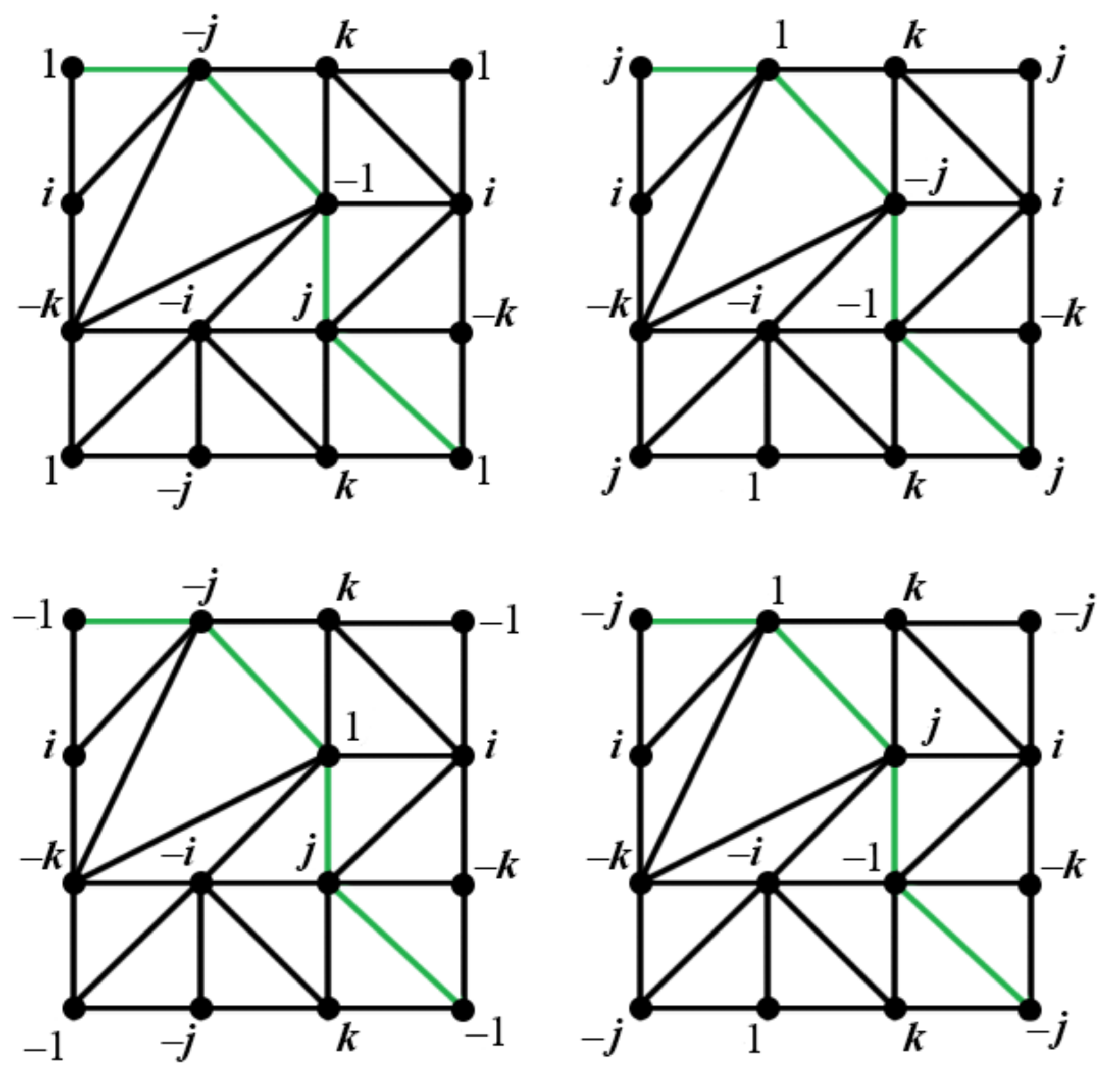
Lemma 1.

Under the action of the quotient group $D_8/Z\left(D_8\right)$ of the dihedral group $D_8=D_8(1,i,-1,-i)$ by its center, on the set Λ, the orbit of the triangulation $T\left(G\right)$ consists of the four vertex-labeled triangulations shown in Figure 8b as Series 1. Moreover, both pairs of triangulations appearing in the same row of Figure 8b do not have any face in common; they are complementary of each other as simplicial 2-complexes with the same graph G.

Consider the automorphism $\left(ij\right)(-i-j)$ of the graph G. This graph automorphism moves the triangulation $T\left(G\right)$ to the triangulation $\left(ij\right)(-i-j)·T\left(G\right)$, shown in the left-hand side of the upper row of Figure 9, taking the (red) cycle $(1,i,-1,-i)$ onto the (green) cycle $(1,j,-1,-j)$ (check with Figure 7). We process the triangulation $\left(ij\right)(-i-j)·T\left(G\right)$ in the same way as we did with the triangulation $T\left(G\right)$ in the proof of Lemma 1 (which immediately precedes the statement of the lemma), swapping i and j, $-i$ and $-j$, and switching from the red to the green color. This leads to Series 2 of four pairwise different toroidal triangulations, shown in Figure 9. Each of them is obtained as effect of the graph automorphism $\left(ij\right)(-i-j)$ on the corresponding triangulation of Figure 8b. The groups $D_8$ and $D_8/Z\left(D_8\right)$ are defined similarly as for $T\left(G\right)$ in the proof of Lemma 1.

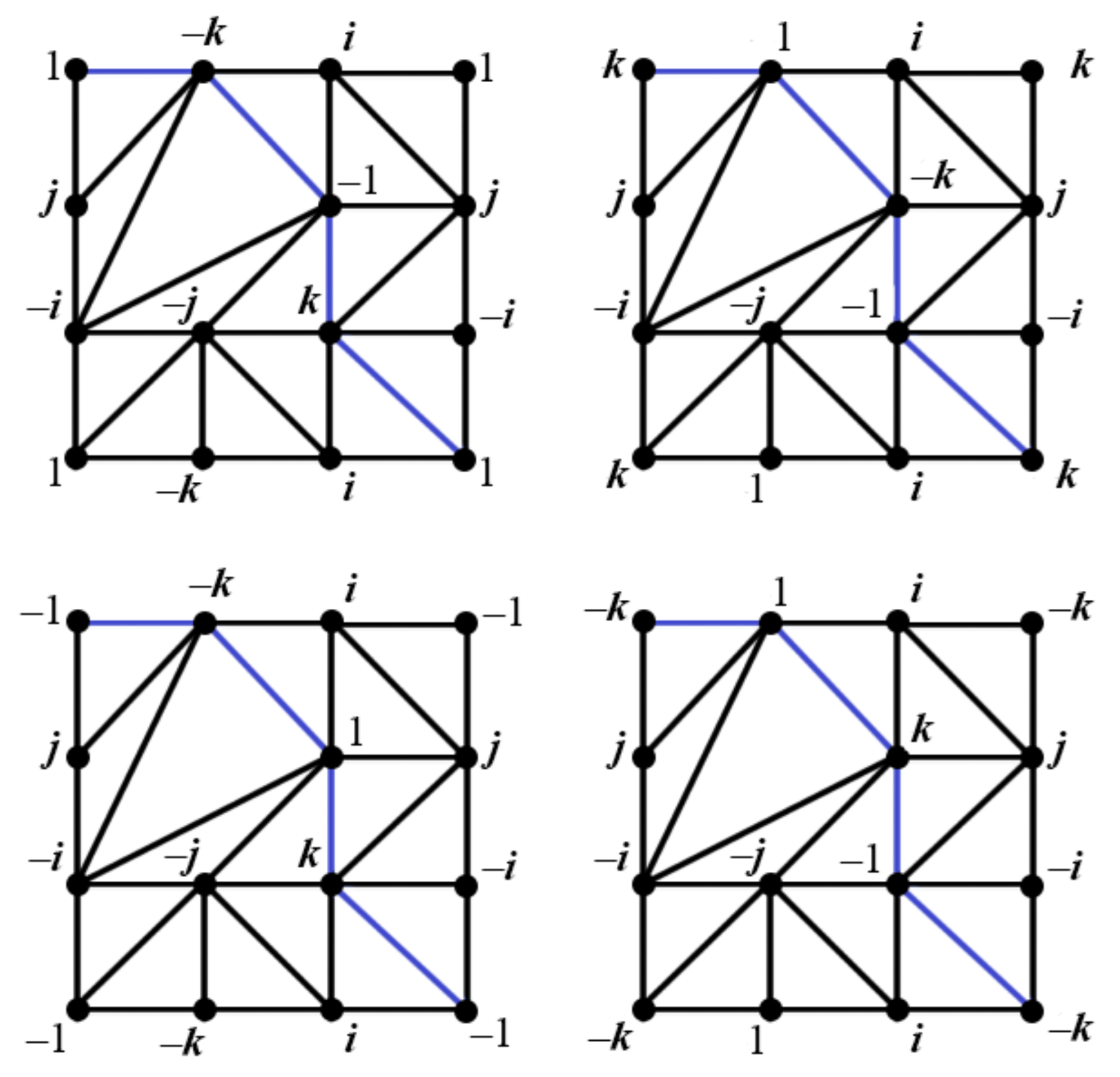
Similarly, the triangulation $\left(ik\right)(-i-k)·T\left(G\right)$ is presented in the left-hand side of the upper row of Figure 10, with the (blue) cycle $(1,k,-1,-k)$ in place of the (red) cycle $(1,i,-1,-i)$ in Figure 8b. We treat the triangulation $\left(ik\right)(-i-k)·T\left(G\right)$ in the same way as $T\left(G\right)$ in the proof of Lemma 1, swapping i and k, $-i$ and $-k$, and switching from the red to the blue color. The groups $D_8$ and $D_8/Z\left(D_8\right)$ are defined similarly as for $T\left(G\right)$ in the proof of Lemma 1. We thus obtain Series 3 of four pairwise different toroidal triangulations, shown in Figure 10.

Theorem 2.

There are precisely 12 triangulations of the torus with the vertex-labeled graph $G=K_{2,2,2,2}$, presented in Figure 8b, Figure 9 and Figure 10, all isomorphic but pairwise different as vertex-labeled triangulations. They are obtained from the three triangulations, $T\left(G\right)$ (Figure 7), $\left(ij\right)(-i-j)·T\left(G\right)$, and $\left(ik\right)(-i-k)·T\left(G\right)$, by the action of the quotient group $D_8/Z\left(D_8\right)$ of the dihedral group $D_8$ by its center, where the corresponding dihedral group $D_8$ stands for the graph-automorphism group of the (undirected) red cycle $(1,i,-1,-i)$ (Figure 8b), green cycle $(1,j,-1,-j)$ (Figure 9), and the blue cycle $(1,k,-1,-k)$ (Figure 10), respectively. Moreover, all the six pairs of triangulations in the same row of Figure 8b, Figure 9 and Figure 10 do not have any face in common; they are complementary of each other as simplicial 2-complexes with the same vertex-labeled graph G.

Proof. 

Observe that Figure 9 [respectively, Figure 10] is obtained from Figure 8b by swapping i and j, $-i$ and $-j$ [respectively, i and k, $-i$ and $-k$] in each of the four diagrams, and switching from the red to the green [respectively, blue] color. Thus, analogs of Lemma 1 still hold for the dihedral groups $D_8=D_8(1,j,-1,-j)$ and $D_8(1,k,-1,-k)$. Thus, the four triangulations in Figure 9 [respectively, Figure 10] are pairwise different as well as the four triangulations in Figure 8b. Finally, it can be easily verified that any pair of triangulations taken from Figure 8b and Figure 9, or Figure 8b and Figure 10, or Figure 9 and Figure 10 are different as triangulations with the vertex-labeled graph G. Thus, we have identified 12 pairwise different triangulations of the torus with the graph G. There are no more different triangulations, by Equation (4). □

Remark 1.

It is not hard to verify that the cycle $C_5$ is the only, up to isomorphism, self-complementary graph (that is, a graph which is isomorphic to its complement) homeomorphic to the 1-torus (that is, a circle); see Figure 1. In this specific case we have: ${\mathbb{K}}^1=K_5$ (the complete graph with 5 vertices), $\mathsf{\Gamma }\equiv \mathrm{Aut}\left(K_5\right)\equiv S_5$, $\mathrm{Aut}\left(C_5\right)\equiv D_{10}$, $P\left(x\right)=x^9$, ${\int }_0^{1}P\left(x\right)dx=1/10$. Thus, by Theorem 1 (III), $1/10=\left|\mathsf{\Lambda }\right|/|S_5|$, whence $\left|\mathsf{\Lambda }\right|=5!/10=12$ is the number of different vertex labelings of $C_5$. It is not hard to verify that those 12 different labeled graphs split into six pairs of cycles which are the complementarities of each other in each pair (see an example in Figure 1).

Therefore, there exist exactly six pairs of mutually complementary simplicial 1-complexes homeomorphic to the 1-torus, which have a cycle of length 5 as underlying simplicial 1-complex. Analogously, $T\left(G\right)$ in Figure 2 (left) is the only, up to isomorphism, self-complementary simplicial 2-complex (that is, a simplicial 2-complex which is isomorphic to its complement) homeomorphic to the 2-torus [19]. Finally, as an intriguing coincidence, there are exactly 6 pairs of mutually complementary simplicial 2-complexes homeomorphic to the 2-torus, which have as underlying simplicial 2-complex the triangulation $T\left(G\right)$.

7. Conclusive Remarks

Our approach to studying the 8-vertex triangulation $T\left(G\right)$ of the torus with the graph $G=K_{2,2,2,2}$ (Figure 2, left) can be briefly summarized as follows. The graph G with the labels removed is known to embed in the torus uniquely up to isomorphism, producing the triangulation $T\left(G\right)$. Using symmetry properties of G and $T\left(G\right)$, Theorem 1 (III) enables us to calculate the number, 12, of pairwise different (triangular) embeddings of the vertex-labeled graph G in the torus. Furthermore, the algebraic approach proposed in this paper enables us to generate the 12 embeddings explicitly in the form of graphics (Figure 8b, Figure 9 and Figure 10), for the first time without computer assistance. For this, we think of the graph G as the (extended) Cayley graph G of the quaternion group $Q_8$ (Figure 7) and observe that the dihedral group $D_8/Z\left(D_8\right)$ of the automorphisms of the cycle $(1,i,-1,-i)$ (with the directions removed) factored by its center, acting on the set $\mathsf{\Lambda }$, moves $T\left(G\right)$ to some 4 pairwise different triangulations, including $T\left(G\right)$ itself (Figure 8b). We also observe that the same construction applies to the triangulations $\left(ij\right)(-i-j)·T\left(G\right)$ and $\left(ik\right)(-i-k)·T\left(G\right)$ in place of $T\left(G\right)$ (Figure 9 and Figure 10). Totally, we obtain $4·3=12$ pairwise different triangulations of the torus with the vertex-labeled graph G.

As far as graph coloring topics go, we observe first that the operation of converting the graph $G=K_{2,2,2,2}$ into the Cayley graph of $Q_8$ (Figure 7) makes the graph Grünbaum colored (see a review [1]), which means that the edges of the graph are 3-colored so that each face of the triangulation $T\left(G\right)$ has all the three colors in its boundary edges. 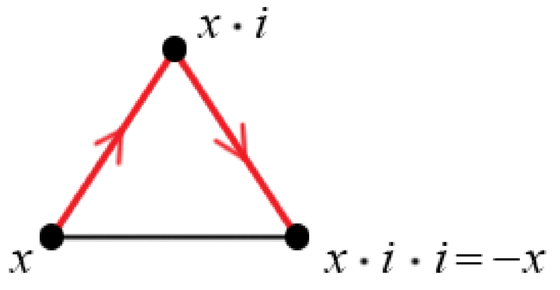Moreover, observe that any cycle of G (Figure 7) with length 3 has all the 3 colors in its edges, and thus any triangulation with the graph G is Grünbaum colored. Observe that Grünbaum coloring entails that edges with the same color (red, for instance) are never neighboring around any vertex of the triangulation, which prevents us from algebraic meaninglessness; for example, it prevents the vertices x and $x·i·i$ ($=-x$) from being adjacent in G, for any $x\in Q_8$; see Figure 11.

Finally, we give a geometric interpretation of Theorem 2 which will be useful in the future research. In fact, the 12 toroidal vertex-labeled triangulations, stated in Theorem 2, are realized geometrically as noble toroidal 2-dimensional polyhedra in the 2-skeleton of the 16-cell in ${\mathbb{R}}^4$; see [2,13]; their difference as vertex-labeled toroidal triangulations ensures that the corresponding 12 polyhedra are different as point-sets in ${\mathbb{R}}^4$. It would be interesting to verify if the 12 polyhedra are all isometric and, if yes, find isometric transformations of ${\mathbb{R}}^4$ which move the 12 polyhedra between themselves. Additionally, we plan to realize the 12 polyhedra in a Schlegel diagram of the 16-cell; this will lead to new toroidal polyhedra in ${\mathbb{R}}^3$ (as discussed in the Introduction).