Optical Inspection Systems for Axisymmetric Parts with Spatial 2D Resolution

Abstract

The article proposes a solution to the problem of increasing the accuracy of determining the main shaping dimensions of axisymmetric parts through a control system that implements the optical method of spatial resolution. The influence of the projection error of a passive optical system for controlling the geometric parameters of bodies of revolution from the image of its sections, obtained by a digital camera with non-telecentric optics, on the measurement accuracy is shown. Analytical dependencies are derived that describe the features of the transmission of measuring information of a system with non-telecentric optics in order to estimate the projection error. On the basis of the obtained dependences, a method for compensating the projection error of the systems for controlling the geometry of the main shaping surfaces of bodies of revolution has been developed, which makes it possible to increase the accuracy of determining dimensions when using digital cameras with a resolution of 5 megapixels or more, equipped with short-focus lenses. The possibility of implementing the proposed technique is confirmed by the results of experimental studies.

1. Introduction

Currently, production efficiency depends on the ability to control the quality of the processed workpieces in a timely manner, the condition of technological equipment and the progress of technological processes at all stages of production. To solve these problems, it is proposed to use optoelectronic devices (including machine vision systems), which make it possible to create automated control systems for various industries [1].

As examples of the use of tools that implement the optical method of control, one can cite the tasks of assessing the cryolite ratio [2], determining the position of the electrodes of ore-thermal furnaces [3] in the metallurgical industry, assessing the efficiency of flotation [4] at obage fabrics, monitoring of self-oscillations in the process of cutting materials based on the registration of the light field [5] and roughness measurement [6,7] in mechanical engineering. Technical vision systems are also used in studies of the mechanical properties of bulk materials [8,9].

The problem of automated control of geometric parameters is an urgent one [10]. Currently, optoelectronic measuring systems have been implemented that implement the projection method [11] and use telecentric optical systems with a collimator illumination system [12]. The main advantage of telecentric optics is a constant magnification factor over the entire operating range and, therefore, the absence of perspective distortions for extended objects, but at the same time, its use greatly increases the cost of the system, limits layout solutions (product inspection only in transmitted light) and the control area to 340 mm, determined by the field of view of existing lenses. The use of digital cameras with non-telecentric optics makes it possible to remove these restrictions. As examples, we can consider the control of the geometry of the current-carrying rods of electrolyzers [13] in metallurgy and the nature of chip formation [14] in the machine-building industry.

The use of active control systems with structured illumination is known [15]; however, an example of a significant drawback of the presented system is the determination of the size of the product in only one section. Comprehensive control of spatial geometry is provided by active optical 3D scanning systems, individual samples of which are certified as measuring instruments [16,17]; however, problems with the control of products with a surface with a pronounced indicatrix of reflection (typical for mechanical engineering products) increase digitization errors [18].

Thus, it can be noted that the use of passive projection systems that implement the spatial resolution method for solving problems of controlling the main shaping dimensions of axisymmetric objects is a promising direction of development. The use of digital cameras with entocentric optics in such systems makes it possible to reduce the cost of control systems and expand their functionality by increasing the variety of possible layout solutions that allow working in both transmitted and reflected light. The latter is an important condition for their use in conjunction with mirror converters, [19] the use of which meaning it is possible to solve the problem of compensating for the positioning error without increasing the number of cameras.

2. Statement of Research Objectives

The main problem of using control systems with entocentric optics for solving problems of controlling the geometric parameters of products is the dependence of the results on many external factors. These include aberrations of the optical system, errors in determining coordinates, positioning of the control object, extraneous illumination, refraction of the medium etc. with the relative position of the control object and the digital camera, and taking into account the imperfection of the optical system, the calibration procedure of the control systems is used [20,21]. Calibration techniques are constantly being improved [22,23,24] and allow for a reduction in systematic error in determining the size of products from their images to a value equivalent to 1–2 px for digital cameras with a resolution of up to 5 Mp, equipped with long-focus lenses. Together with the method of complex error compensation [25], which compensates for background illumination errors and noise components, they provide the ability to control flat products with an error of up to 0.1%.

If until recently digital cameras with a resolution of 0.3–2 Mp were used (in 2017—85% [26]), then the current trend is to increase the resolution of cameras to 5 … 10 Mp [27], and, in the near future, up to 16 … 25MP. The use of high-resolution cameras makes it possible to expand the application of machine vision systems to the tasks of controlling geometric parameters, providing the ability to control with a relative error of less than 0.1%.

However, an increase in resolution leads to the fact that when measuring the dimensions of bodies of revolution, previously imperceptible components of systematic errors appear in the projection, in which the visible image is not located in the plane of symmetry of the part (Figure 1). In this regard, the analysis of the sources of such errors and methods of their compensation becomes an urgent task of the study.

A feature of the formation of an image of bodies of revolution in reflected light by an entocentric system (Figure 2) is that the observed image is not located in the plane of symmetry but is displaced by a distance of l along the optical axis towards the camera. This leads to the fact that, on the one hand, the observed size d is less than the controlled size of the section D, but it is located closer to the calibration plane (coinciding with the axis of symmetry), which leads to a change in the linear increase in V for the observed size d upward. In addition, the displacement of the body of revolution relative to the optical axis by a distance y leads to the rotation of the image by an angle α. Figure 2 shows a geometric model of the formation of an image of an axisymmetric part by entocentric optics for f = 7 mm, L = 200 mm and D = 100 mm. For clarity of presentation of changes in the main parameters, they are shown in Figure 2 next to their corresponding designations.

To assess the influence of these factors on the error in determining the dimensions, we determine the values of these parameters.

Figure 2 shows the fixed inverse image of the section of the body of revolution D has an apparent size d

$$\mathrm{d}=\mathrm{D}·\sqrt{1-{\left(\frac{\raisebox{1ex}{$\mathrm{D}$}\!\left/ \!\raisebox{-1ex}{$2$}\right.}{\mathrm{L}-\mathrm{f}}\right)}^2}$$

(1)

where: L—working distance, f—focal length.

The visible image is smaller than the object, and this difference only grows with decreasing focal length. In this case, the image is displaced along the optical axis by

$$\mathrm{l}=\frac{{\mathrm{D}}^2}{4·\left(\mathrm{L}-\mathrm{f}\right)}.$$

(2)

Observation angle γD of controlled size D.

$${\mathsf{\gamma }}_{\mathrm{D}}=\mathsf{а}\sin \left(\frac{\raisebox{1ex}{$\mathrm{D}$}\!\left/ \!\raisebox{-1ex}{$2$}\right.}{\mathrm{L}-\mathrm{f}}\right)$$

(3)

All this leads to errors in estimating the size of products. The dependences of the calibration errors δv, the projection error δd and the total error δ∑ on the ratio of the determined dimensions D to the width of the field of view B are shown in Figure 3 for 12 and 25 mm lenses.

It can be seen from the graphs that when the size of the test object almost completely coincides with the field of view, the error for a 12 mm objective can reach 1%, and for a 25 mm objective—0.25%. Thus, when measuring the dimensions of parts that occupy most of the field of view of a digital camera, the influence of these errors can be considered significant for the control of products according to 8–9 qualities. With product sizes less than 50% of the field of view, the considered error for a 25 mm lens is ~0.07% and becomes insignificant for cameras with a resolution of up to 5 Mp.

3. Materials and Methods

Numerical simulation and experimental research was carried out based on the use of cameras for image registration: Basler Pilot piA2400-17 (sensor: CCD 2/3 “; resolution 2456 × 2058), with Ricoh FL-CC2514-2M lenses (f = 25 mm), Ricoh FL- HC0612A-VG with f = 12 mm; ACE acA640-120gm (sensor: CCD 1/4 “; resolution 659 × 494) and 5,0 Mп USB camera (sensor: CMOS 1/2.5”, resolution 2592 × 1944) with Computar M1214-MP2 lens with f = 6 mm.

The software implementation was carried out in the LabVIEW environment using the Vision library (technical vision module) [28]. The built-in calibration function was used based on the image obtained using the Calibration Training utility against a standard point pattern with a step of 10 × 10 mm, made by laser graphing with an error of no more than 0.01 mm (Figure 4a).

For control, 3 samples of parts were made, which were shafts 75 mm long with four separated grooved surfaces Ø 15, 20, 25 mm (Figure 4b). The actual dimensions of the samples were estimated using a digital micrometer CDWAS 0–25 Δ = ±0.002 mm and a linear displacement transducer with a rod LIR14-20-01 of the 2nd accuracy class with a digital display device LIR-510A-00 using plane-parallel gauge blocks.

The position of the test object, which affects the accuracy of the calibration procedure, was estimated using the developed software in the LabVIEW environment [29], the operation algorithm of which is described in [30].

The study of the error compensation technique was carried out in reflected light. Figure 5 shows fragments of experimental studies, illustrating the comparative results of the evaluation of the sample sizes with calibration—Distortion Model: Polynomial (Kl, K2, K3), using the developed compensation algorithms and without these same algorithms.

4. Results

To determine the amount of compensation, you need to derive the inverse relationship. The initial data are the parameters f,${\mathrm{D}}_{\mathrm{k}}$—the calculated size, based on the calibration data in the symmetry plane ${\mathrm{n}}_{\mathrm{d}}$—the number of pixels that make up the image of the visible size ${\mathrm{d}}^{\prime }$.

The following dependencies can be used to compensate for the perspective error:

$$\mathrm{D}={\mathrm{D}}_{\mathrm{K}}·\cos \left({\tan }^{-1}\left(\frac{{\mathrm{d}}^{\prime }}{2\mathrm{f}}\right)\right)$$

(4)

or

$$\mathrm{D}={\mathrm{D}}_{\mathrm{K}}·\cos \left({\tan }^{-1}\left(\frac{{\mathrm{D}}_{\mathrm{HK}}}{2(\mathrm{L}-\mathrm{f})}\right)\right)$$

(5)

where ${\mathrm{D}}_{\mathrm{HK}}$ is the diameter obtained as a result of measurements from the image.

To compensate for the manifestation of a perspective error in the horizontal plane, it is necessary to take into account the change in the linear magnification factor when mixing the visible image along the x axis by l, which can be determined by formula (3).

The cross section is observed at an angle ν, which can be determined from the dependence

$$\mathsf{\nu }={\sin }^{-1}\frac{\mathrm{z}}{\mathrm{L}-\mathrm{f}}$$

(6)

where z is the displacement relative to the optical axis along the axis of symmetry of the body of revolution.

The change in Δl can be determined from the dependence

$$\mathsf{\Delta }\mathrm{l}=\frac{{\mathrm{D}}^2\left(1-\cos \mathsf{\nu }\right)}{4·\left(\mathrm{L}-\mathrm{f}\right)}.$$

(7)

To take into account the displacements of the shaft axis in the vertical plane relative to the axis of symmetry of the body of revolution by y, we define the rotation of the observed section by the angle α

$$\mathsf{\alpha }={\tan }^{-1}\left(\frac{\mathrm{y}}{\mathrm{L}-\mathrm{l}}\right).$$

This will displace the image horizontally and resize the image by

$${\Delta }_{\mathsf{\alpha }}=\mathrm{D}·\cos \mathsf{\alpha }.$$

(8)

Figure 5 shows a graph of the dependence of the relative error in determining the dimensions of bodies of revolution in case of violation of the condition of crossing the axis of symmetry of the body of rotation of the optical axis of a digital camera, presented in a relative form of dependence for lenses: with f = 6 mm L = 39 mm and f = 12 mm and L = 145 mm.

Notes for algorithm for complex compensation of errors:

1. correction of the horizontal component, takes into account the rotation of the test object relative to the vertical axis by changing the parameter z of expression (7).

2. correction, takes into account the violation with respect to the condition of perpendicularity of the test object of the optical axis of the digital camera and can be determined by the expression ${\Delta }_{\mathsf{\alpha }}=\mathrm{D}·\cos \mathsf{\beta }$, where β is the angle of inclination of the test object.

3. correction, taking into account the position of the test object, can be performed based on the linear magnification measurement dependence, which can be calculated by the formula ${\mathsf{\delta }\mathrm{V}}_{\mathrm{P}}=\frac{{\mathrm{X}}_{\mathrm{P}1}-\mathrm{f}}{{\mathrm{X}}_{\mathrm{P}}-\mathrm{f}}=\frac{{\mathrm{X}}_{\mathrm{P}}\pm \Delta \mathrm{X}-\mathrm{f}}{{\mathrm{X}}_{\mathrm{P}}-\mathrm{f}}$, where: ΔX—displacement of the controlled rod

Based on the obtained regularities, an algorithm for image processing and correction of the calculated values was developed for the complex compensation of errors in the control system of axisymmetric products, which is shown in Figure 6.

To assess the developed compensation technique, we calculate the main parameters shown in Figure 2. The results of modelling the error compensation process are presented in

Table 1. Results of numerical simulation of compensation of projection error of the system for controlling the dimensions of axisymmetric objects.

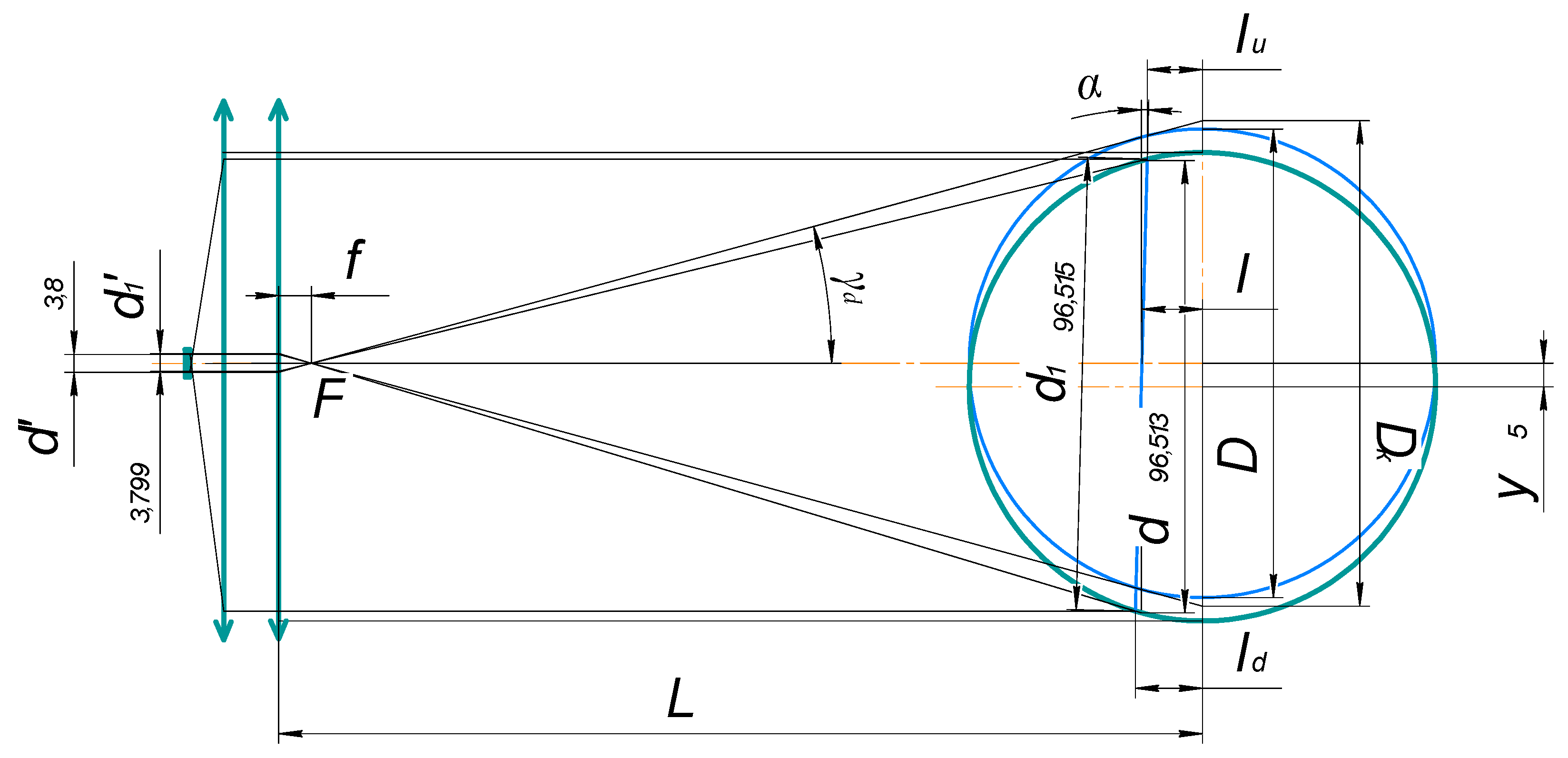
f, mm	D, mm	L, mm	γ, °	V	l, mm	D, mm	d’, mm	Dk, mm	${\gamma }_p$, °	$D_p$, mm
6	49.27	72	21,916	0.0909	9.1952	45.709	4828	53,108	21,916	49.27
6	30.77	72	13,480	0.0909	3.5863	29.922	2876	31,642	13,480	30.77
6	25.38	72	11,085	0.0909	2.4399	24.906	2351	25,863	11,085	25.38
6	15.43	72	6712	0.0909	0.9018	15.324	1412	15.5363	6712	15.43
f, mm	D, mm	L, mm	γ, °	V	l, mm	m	d’, mm	Dk, mm	${\gamma }_p$, °	$D_p$, mm
f	D	L	α	V	l	d		Dk	${\mathsf{\alpha }}_p$	${\mathrm{D}}_p$
12	49.27	153	10,062	0.0851	4.3041	48.512	4258	50,040	10,062	49.27
12	30.77	153	6264	0.0851	1.6787	30.586	2634	30,955	6264	30.77
12	25.38	153	5163	0.0851	1.1421	25.277	2168	25,483	5163	25.38
12	15.43	153	3136	0.0851	0.4221	15.406	1315	15,453	3136	15.43

. Its results show the possibility of full compensation of the considered errors for an ideal optical system.

In Figure 7—graphs of errors in determining the dimensions of a sample with a nominal Ø 25 mm: using only the calibration procedure (Cal.), using the projection error compensation algorithm (CA) and complex compensation (CC) errors for digital cameras whith f = 25 mm and f = 12 mm entocentric optics. The error graph for a camera with an f = 12 mm lens additionally shows a constant factor calibration (Const.) to clearly demonstrate lens distortion. Examples of measurement results with 60 sampling points are given.

The results of a quantitative assessment of the results of the correction are presented in

Table 2. Evaluation of methods for correction of dimensions for f = 25 mm.

Parameters	Calibration (Cal.)			Compensation of Projection Error (CA)			Compensation of Projection Error + Position of Test-Object			Complex Compensation (CC)
f, mm	25		12	25		12	25		12	25	12
m	20	48	48	20	48	48	20	48	48	48	48
$\overline{\mathrm{M}}$, mm	0.079	0.073	0.224	0.042	0.042	0.118	0.034	0.033	0.098	−0.004	0.006
$\overline{\mathrm{S}}$,	0.079	0.081	0.237	0.048	0.053	0.135	0.041	0.046	0.118	0.026	0.057
δ *, mm	0.174	0.171	0.489	0.107	0.112	0.285	0.090	0.098	0.242	0.055	0.11

* t_0,04;48 = 2112; t_0,04;20 = 2204.

. A column was added showing correction results, combining projection error compensation and test object position error.

While analyzing the obtained values, it can be concluded during the use of cameras with a resolution of 5 Mp with long-focus lenses (with f = 25 mm and more) that the projection error is comparable to the positioning error, and the dominant error is the binarization error. For a 5-megapixel camera with a short-focus lens f = 12 mm, the projection error and displacement errors of the body of revolution have a significant effect on the accuracy of determining the dimensions of the bodies of revolution. Their compensation practically eliminates the systematic component, which decreases from approximately 1% to 0.024%, which is less than ½ pix for the camera under consideration. It can be seen from the graphs that, as before, the dominant random component is the image binarization error equal to ±1.5 pix.

Figure 8 shows an example of comparing different calibration algorithms for a camera with lenses f = 25 mm and f = 25 mm. The object position error for 23 control points has not been corrected for clarity. The results of a quantitative assessment of the results of the correction are presented in

Table 3. Errors in determining the dimensions of a 25 mm diameter roller at different calibrations with a lens with f = 25 and 12 mm at m = 20.

Parameters	Sim.	Div.	Pol. k1	Tan. k1	Pol. k3	Tan. K3
f = 25 mm
$\overline{\mathrm{M}}$, mm	−0.002	0.014	0.008	0.009	−0.002	−0.001
$\overline{\mathrm{S}}$, mm	0.049	0.035	0.036	0.033	0.036	0.035
δ*, mm	0.109	0.078	0.080	0.072	0.080	0.078
f = 12 mm
$\overline{\mathrm{M}}$, mm	0.05	−0.003	0.018	0.020	0.010	0.034
$\overline{\mathrm{S}}$, mm	0.092	0.025	0.030	0.034	0.033	0.044
δ *, mm	0.203	0.056	0.066	0.075	0.072	0.097

* t_0,04;20 = 2204.

.

Comparison of the results of image correction for a lens with f = 25 mm shows that the use of standard calibrations of optical distortions NI with three coefficients makes it possible to almost completely eliminate the systematic component determined by distortions of the optical system ⁻M = 0.001 … 0.002 mm. The random component is mainly determined by the image binarization errors. The division of the field of view into two binarization areas (top and bottom) is insufficient. For a lens with f = 12 mm, due to the absence of image rotation, the Divison calibration provided a lower systematic error, with practically equal values of the random error, the spread of the values of which is within the statistical error of the estimate.

The effect of threshold binarization values can be clearly represented in Figure 9, from which it can be seen—when the threshold values are changed by 3 … 4 units at the top of the image from 180/255 to 183/255 and from 140/255 to 136/254 at the bottom, results in a change in ± 1–2 pxs.

A numerical estimate of the influence of the binarization threshold values during measurement of the dimensions of a detail for a 5MP camera with a long-focus lens f = 25 mm is given in

Table 4. Evaluation of the effect of binarization threshold values for a long-focus lens with f = 25 mm.

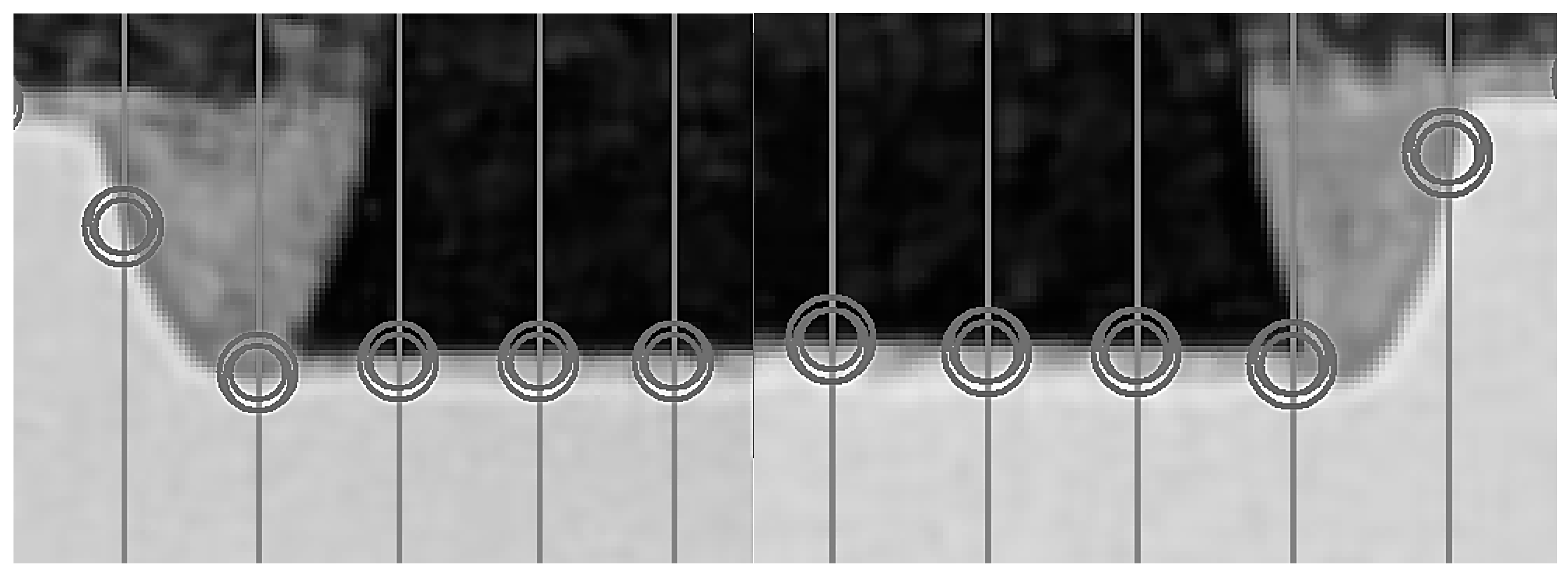
Parameters	180/255 &140/255		183/255 & 136/254
Bias Compensation	No	Yes	No	Yes
$\overline{\mathrm{M}}$, mm	0.036	0.006	0.035	0.005
$\overline{\mathrm{S}}$, mm	0.049	0.033	0.044	0.027
δ *, mm	0.108	0.073	0.098	0.059

* t_0,04;46 = 2114.

.

Due to the irregularity of illumination at the edges of the image, an error arises in determining the dimensions according to a fixed threshold binarization value, which affects the accuracy of determining the dimensions. The operation of subtracting the background does not always compensate for this component due to the appearance of a shadow when installing a part, which is absent when fixing the background.

The filtering procedure eliminates the noise component. Figure 10 and

Table 5. Evaluation of filtration calibration methods for a telephoto lens f = 25 mm.

Parameters	No Filter	Filter
		Gausian			Smoothing
Kernel		3	5	7	3	5	7
$\overline{\mathrm{M}}$, mm	0.050	0.041	0.035	0.037	0.039	0.028	0.023
$\overline{\mathrm{S}}$, mm	0.063	0.051	0.045	0.048	0.049	0.041	0.043
δ *, mm	0.140	0.114	0.098	0.107	0.107	0.089	0.096

* t_0,04;46 = 2114.

demonstrate the application of Gausian and Smoothing filters with kernel sizes 3, 5, 7. Slight blurring of the image smoothed out the random noise component and surface flare.

The results of the study show that the use of filters can reduce the confidence interval by up to one and a half times. The values obtained show the preferred use of a 5-kernel smoothing filter.

The results of studying the compensation of systematic errors of a 0.3 Mp camera with an f = 6 mm lens at L = 275.5 mm are shown in Figure 11 and in

Table 6. Errors in determining the dimensions of a 25 mm diameter roller in the absence and use of compensation algorithms for a 0.3 Mp camera with a lens f = 6 mm.

Parameters	Constant Koefficient (Const.)	No Compensation (Cal.)	Compensation of Projection Error (CA)	Complex Compensation (CC)	Complex Compensation + Developer Cal. (DDC+CC)
$\overline{\mathrm{M}}$, MM	−0.052	0.026	0.005	0.004	0.031
$\overline{\mathrm{S}}$, MM	0.118	0.080	0.075	0.075	0.012
δ *, MM	0.249	0.169	0.158	0.158	0.110

* t_0,04;46 = 2114.

. The developed distortion compensation (DDC) model based on the use of the image space sampling algorithm [31] has been added to the previously considered algorithms with standard NI calibrations.

The results of comparison use the standard calibration Distortion Model: Polynomial (Kl, K2, KZ) and the developed one are shown in Figure 12 and

Table 7. Measurement errors of 15, 20 and 25 mm with a 0.3 Mp camera with an f = 6 mm lens using standard calibration and developed.

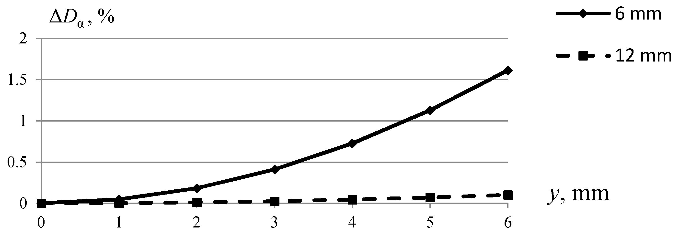
Parameters	15 mm		20 mm		25 mm
Distortion Correction Methods	Standard	Developed	Standard	Developed	Standard	Developed
$\overline{\mathrm{M}}$, mm	−0.012	0.042	−0.003	−0.021	0.029	−0.005
$\overline{\mathrm{S}}$, mm	0.052	0.050	0.062	0.041	0.062	0.042
δ *, mm	0.118	0.112	0.139	0.092	0.139	0.095

* t_0,04;20 = 2204.

.

Analyzing the obtained values, it can be concluded during the use of cameras with low resolution that the projection error is comparable to the positioning error, and the dominant error is the binarization error.

Investigation of algorithms for compensation of systematic errors for cameras with a resolution of 5.0 Mp was carried out using a USB camera with a 1/2.5” sensor camera with a Ricoh FL-HC0612A-VG f = 6 mm lens at L = 114.8 mm.

The research results are shown in Figure 13 and in

Table 8. Errors in determining the dimensions of the roller D_nom = 25 mm in the absence and use of compensation algorithms for a 5 Mp camera with f = 6 mm.

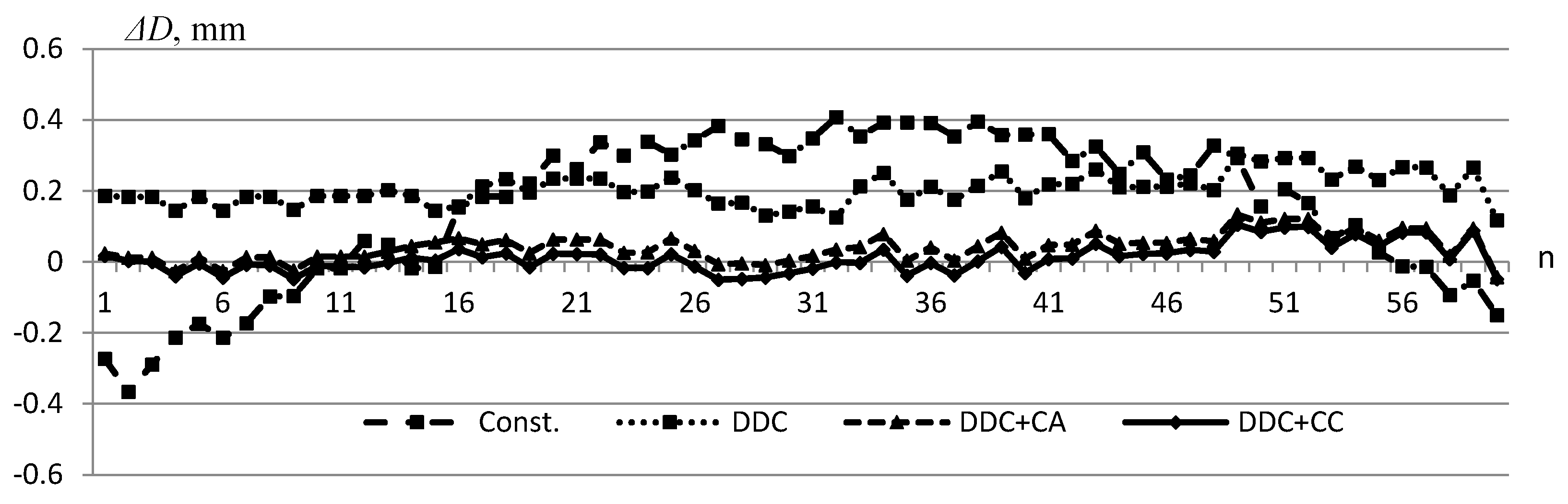
Parameters	Constant Coefficient (Const.)	No Compensation (DDC)	Compensation of Projection Error (DDC+CA)	Complex Compensation (DDC+CC)
$\overline{\mathrm{M}}$, MM	0.154	0.205	0.042	0.011
$\overline{\mathrm{S}}$,	0.264	0.211	0.057	0.042
δ *, MM	0.559	0.448	0.122	0.089

* t_0,04;46 = 2114.

.

To assess the repeatability of measurement results by a control system with a 5-megapixel camera and f = 6 mm lens, the measurement errors of parts of different sizes were estimated. The results of measuring the diameters of parts with nominal Ø 15, 20 and 25 mm were compared using the developed calibration of the PDI. The results are shown in Figure 14 and

Table 9. Errors in determining the dimensions of the rollers during usage of compensation algorithms with a 5 Mp camera (f = 6 mm).

Parameters	Dnom
	15 mm	20 mm	25 mm
$\overline{\mathrm{M}}$, mm	0.003	0.001	0.001
$\overline{\mathrm{S}}$,	0.033	0.032	0.035
δ *, mm	0.072	0.070	0.077

* t_0,04;20 = 2204.

.

5. Discussion

Compensation for systematic projection errors in the control of the main shaping dimensions of axisymmetric parts by the spatial method of optical radiation with 2D resolution from the images of their sections, when using digital cameras with lenses with a fixed focal length in transmitted light, is possible based on the obtained analytical dependences, taking into account the position of the test object and projection component errors. This allows for an increase in the accuracy of determining the main shaping dimensions in reflected light with non-collimated illumination for digital cameras with a resolution of 5 Mp or more, with lenses where the focal length is approximately 1.5 or more of the frame diagonal (short-focus optics).

During analyzation of the results obtained, it can be concluded that with a significant distortion of the Ricoh FL-HC0612A-VG lens, the developed calibration method, based on the use of the image space sampling algorithm, can reduce the confidence interval by more than four times.

Reduction of the error to 0.05% is possible with the use of more advanced image binarization techniques [32,33].

6. Conclusions

The works were carried out to compensate the projection error in the control of axisymmetric parts, solving the problem of increasing the accuracy of determining the main shaping dimensions by optical control systems by the geometric method, using digital cameras with a fixed focal length and receiving measurement information from the image of sections.

Experimental studies have shown the possibility of increasing the accuracy of measuring the diameters of bodies of revolution through control systems equipped with digital cameras with a resolution of 5 Mp or more, with short-focus optics, by an algorithmic method based on taking into account the peculiarities of transferring measurement information about the geometry of bodies of revolution by entocentric optics.

The developed method and software for complex compensation of errors in deter-mining the main shaping geometry of axisymmetric objects allows for a reduction in error in determining dimensions in reflected light with non-colimated illumination for short-focus optics to Δ = ± 0.1 mm, corresponding to 9–10 accuracy grades for the investigated ranges of sizes of the test object, with a confidence level of 96%.

The problems of compensation of random components of errors should be solved in the future. It will make a full realization of the resolution of modern digital cameras possible, and determination of the position of objects under control in space for their non-fixed position.

References

- Computer Vision: Technologies, Market Prospects. Available online: https://www.tadviser.ru/index.php/Article:_Computer_vision_:_technologies_,_market_,_prospects/ (accessed on 14 March 2021).
- Bazhin, V.Y.; Boikov, A.V.; Ivanov, P.V. Optoelectronic method for monitoring the state of the cryolite melt in aluminum electrolyzers. Russ. J. Non-Ferr. Met. 2015, 56, 6–9. [Google Scholar] [CrossRef] [Green Version]
- Martynov, S.A.; Bazhin, V.Y. Improving the control efficiency of metallurgical silicon production technology. J. Phys. Conf. Ser. 2019, 1399. [Google Scholar] [CrossRef] [Green Version]
- Romachev, A.; Kuznetsov, V.; Ivanov, E.; Jörg, B. Flotation froth feature analysis using computer vision technology. In E3S Web of Conferences; EDP Sciences: Les Ulis, France, 2020; p. 192. [Google Scholar] [CrossRef]
- Maksarov, V.V.; Makhov, V.E. Reduction of defects in the process of formation of preci-sion surfaces of titanium alloy products. J. Phys. Conf. Ser. 2020, 1661. [Google Scholar] [CrossRef]
- Zmarzły, P. Influence of bearing raceway surface topography on the level of generated vibration as an example of operational heredity. Indian J. Eng. Mater. Sci. 2020, 27, 356–364. [Google Scholar]
- Fuqin, D.; Liu, C.; Sze, W.; Deng, J.; Fung, K.; Leung, W.; Lam, E. An illumination-invariant phase-shifting algorithm for three-dimensional profilometry. In Image Processing: Machine Vision Applications V; International Society for Optics and Photonics: Bellingham, DC, USA, 2021; Volume 8300. [Google Scholar] [CrossRef] [Green Version]
- Boikov, A.V.; Payor, V.A.; Savelev, R.V. Technicalvisionsystem for analysing the mechan-ical characteristics of bulk materials. J. Phys. Conf. Ser. 2018, 944. [Google Scholar] [CrossRef]
- Beloglazov, I.I.; Boikov, A.V.; Petrov, P.A. Discrete element simulation of powder sintering for spherical particles. Key Eng. Mater. 2020, 854, 164–171. [Google Scholar] [CrossRef]
- Maksarov, V.V.; Olt, J. Dynamic stabilization of machining process based on local metastability in controlled robotic systems of CNC machines. Zap. Gorn. Inst. 2017, 226, 446–451. [Google Scholar] [CrossRef]
- The Opticline CS Measurement Systems [Electronic Resource]. Available online: https://www.jenoptik.com/products/metrology/opticline-optical-shaft-metrology/opticline%20cs-serie (accessed on 28 March 2020).
- Makhov, V.E. Control of linear dimensions of products based on technologies from “National Instruments”. Izvestiya vysshikh uchebnykh zavedeniy. Priborostroenie 2010, 7, 54–60. [Google Scholar]
- Bazhin, V.Y.; Kulchitskiy, A.A.; Kadrov, D.N. Complex control of the state of steel pins in soderberg electrolytic cells by using computer vision systems. Tsvetnye Met. 2018, 27–32. [Google Scholar] [CrossRef]
- Maksarov, V.V.; Makhov, V.E. Intelligent systems for monitoring and controlling chip for-mation when cutting difficult-to-machine materials. IOP Conf. Ser. Mater. Sci. Eng. 2019, 560. [Google Scholar] [CrossRef]
- Tan, Q.; Kou, Y.; Miao, J.; Liu, S.; Chai, B.A. Model of diameter measurement based on the machine vision. Symmetry 2021, 13, 187. [Google Scholar] [CrossRef]
- Certificate of Type Approval of Measuring Instruments DE.C.27.004.A No. 52362, Optical Coordinate-Measuring Topometric Systems ATOS, Manufacturer GOMmbH, Germany Registration No. 54916-13, Type of Measuring Instruments Approved by Order of the Federal Agency for Technical Regulation and Metrology from September 23, 2013, No. 1110. Available online: https://www.ktopoverit.ru/prof/opisanie/54916-13.pdf (accessed on 14 March 2021).
- Certificate of Approval of Measuring Instruments OS.C.27.004.A No. 75179 Optical Three-Dimensional Scanners RangeVisionPRO, Manufacturer RangeVision Limited Liability Company (Range Vision LLC). Moscow Region, Krasnogorsk, Registration No. 76251-19, the Type of Measuring Instruments Approved by Order of the Federal Agency for Technical Regulation and Metrology Dated September 27, 2019, No. 2316. Available online: https://rangevision.com/company/news/rangevision-pro-ofitsialno-zanesen-v-gosudarstvennyy-reestr-sredstv-izmereniy/ (accessed on 6 June 2021).
- Eldib, I.S.A. Development of a Methodology for Improving the Technological Process of Cold Stamping of Products Based on Optical 3d-Scanning and Numerical Modeling, Dissertation for the Degree of Candidate of Technical Sciences-Specialty 05.16.05 Processing of Metals by Pressure, Moscow, Moscow Polytechnic University, 2020. Available online: https://viewer.rusneb.ru/ru/rsl01010248295?page=1&rotate=0&theme=white (accessed on 6 June 2021).
- Kulchitsky, A.A.; Potapov, A.I.; Smirnov, A.G.; Boykov, V.I. The control system of the geometry of axisymmetric products with an angular mirror converter, Bulletin of higher educational institutions. Instrumentation 2020, 63, 720–726. [Google Scholar]
- Brown, D.C. Close-range camera calibration. Photogramm. Eng. 1971, 37, 855–866. [Google Scholar]
- Tsai, R.Y. A versatile camera calibration technique for high-accuracy 3D machine vision metrology using off-the-shelf TV cameras and lenses. IEEE Int. J. Robot. Autom. 1987, 3, 323–344. [Google Scholar] [CrossRef] [Green Version]
- Zhang, Z. A flexible new technique for camera calibration. IEEE Trans. Pattern Anal. Mach. Intell. 2000, 22, 1330–1334. [Google Scholar] [CrossRef] [Green Version]
- Fitzgibbon, A.W. Simultaneous linear estimation of multiple view geometry and lens distortion. In Proceedings of the 2001 IEEE Computer Society Conference on Computer Vision and Pattern Recognition (CVPR) 2001, Kauai, HI, USA, 8–14 December 2001. [Google Scholar] [CrossRef]
- Antipov, I.T. Mathematical Foundations of Spatial Analytical Phototriangulation; Kartgeocenter-Geodezizdat: Moscow, Russia, 2003; 296p. [Google Scholar]
- Abakumov, I.I.; Kulchitsky, A.A. Compensation of errors of passive optoelectronic monitoring system of geometry. Meas. Tech. 2016, 8, 56. [Google Scholar]
- Industrial Cameras, Technical Features, and Market [Electronic Resource]. Available online: https://industryeurope.com/industrial-cameras-technical-features-and-market/ (accessed on 14 March 2021).
- Muller, R. FRAMOS Market Survey. Available online: https://www.framos.com/en/news/framos-launches-embedded-vision-ecosystem-of-sensor-modules-and-adapters/ (accessed on 5 February 2021).
- Kulchitskiy, A.A.; Kashin, D.A.; Romanova, N.A. The Program for Determining the Position of the Test Object during the Calibration of the Optical Projection System for the Control of Axisymmetric Products. Application No. 2020664591, Date of Receipt November 20, 2020, the Date of State Registration in the Register of Computer Programs November 25. 2020 year. Available online: https://elibrary.ru/download/elibrary_44762850_17629678.PDF (accessed on 6 June 2021).
- Kulchitsky, A.A.; Kashin, D.A.; Smirnov, A.G. The Program for Control of the Dimensions of Axisymmetric Products with Compensation for the Perspective Error of a Single-Channel Optical System. Application No. 2020664591, Date of Receipt November 20, 2020, the Date of State Registration in the Register of Programs for COMPUTER 25.11. February 2020. Available online: https://elibrary.ru/download/elibrary_44443086_50035226.PDF (accessed on 6 June 2021).
- Kulchitsky, A.; Zubareva, A. Reduction of measurement error of axisymmetric parts with an optical system. XIV international Scientific Conference “INTERAGROMASH 2021”. Precis. Agric. Agric. Mach. Ind. 2021, 1, 1–11. [Google Scholar]
- Abakumov, I.I.; Kulchitskiy, A.A. Algorithmic way to compensate for the errors of an automated electronic control system for geometric parameters of objects. In Innovative Systems of Planning and Management in Transport and Mechanical Engineering: Collection of Works of the II International Scientific and Practical Conference Volume II; National Mineral Resources University Mining: St. Petersburg, Russia, 2014; pp. 104–107. [Google Scholar]
- Makhov, V.E.; Potapov, A.I.; Shaldaev, S.E. Investigation of the image boundaries by the contrast extraction method using an optoelectronic system Part 1. Scientific and methodological principles of image border control by the contrast extraction method. Control. Diagn. 2017, 10, 44–51. [Google Scholar]
- Makhov, V.E.; Potapov, A.I.; Shaldaev, S.E. Investigation of the image boundaries by contrast extraction using an opto-electronic system Part 2. Experimental model studies of image boundaries based on wavelet transforms. Kontrol. Diagn. 2017, 11, 4–11. [Google Scholar] [CrossRef]