Abstract
Specific emitter identification involves extracting the fingerprint features that represent the individual differences of the emitter through processing the received signals. By identifying the extracted fingerprint features, one can also identify the emitter to which the received signals belong. Due to differences in transmitter hardware, this fingerprint cannot be duplicated. Therefore, SEI plays an important role in the field of information security and can reduce the information leakages caused by key theft. This method can also be used in the military field to support communication countermeasures via emitter individual identification. In this paper, empirical mode decomposition is carried out for each radar pulse signal, and then the bispectral features are extracted. Dimensionality reduction is carried out according to the symmetry of the bispectral features. The features after dimensionality reduction are input into a one-dimensional LeNet neural network as the fingerprint features of the emitter, and the identification of 10 radar emitter sources is completed. Based on the verification of real signals, the SEI identification strategy in this paper achieved a recognition rate of 96.4% for 10 radar signals, 98.9% for 10 data emitter signals, and 88.93% for 5 communication radio signals.
1. Introduction
Specific emitter identification (SEI) identifies the signal source by analyzing the subtle characteristics of the received signal. Here, subtle features refer to the signal features that can distinguish individuals of the same type of electronic radiation source. Because this identification process is similar to human fingerprint identification, it is called “radio frequency fingerprint (RFF) identification”.
In terms of communication security, due to the popularity of wireless communication terminals, wireless communication networks have become targets of attack. By detecting the subtle characteristics of communication equipment, we can identify disguised intruding communication equipment and guarantee the security of communication networks. For example, a fingerprint database of legal communication devices can be established. If the fingerprints of the detected communication devices are not in the fingerprint database, those devices will be prohibited from accessing the communication network, thereby establishing a network security protection layer on the physical layer. In the field of communication countermeasures, the two basic tasks of communication reconnaissance are positioning and identification. As a major research direction of array signal processing, positioning technology has been widely explored, while research on communication emitter identification remains relatively uncommon. Only by combining both tasks can effective reconnaissance be achieved [1]. With the development of science and technology, SEI will become increasingly important in the field of intelligence.
SEI research is based on feature extraction, and the current main feature extraction methods can be divided into three categories [2]. The first category is statistical fingerprint feature extraction based on signal parameters. Xing proposed a DRC algorithm to divide pulses into different operating modes, and then extract transient RF fingerprint features and modulate RF fingerprint features from the derivative envelope of signals through noise suppression, thus solving the radar identification problem based on RF fingerprints. When the SNR is about 5 dB, the recognition rate is 90% [3]. Reising and Williams et al. extracted statistical parameters such as instantaneous amplitude; instantaneous phase; and instantaneous frequency mean, variance, and kurtosis as individual characteristics of radiation sources, respectively, for transient segments and pilot segments of a GSM signal, WiMax signals and ZigBee signal [4,5,6,7,8]. It has equally been proven experimentally that the time domain statistical parameter features can achieve good individual identification of radiation sources. Among these sources, the statistical parameters of the instantaneous phase have a stronger ability to distinguish different individual radiation sources [4]. In [5], an identification test for GSM mobile phones showed that individual identification performance was able to reach 94% when SNR = 6 dB based on the characteristics of the transient phase statistical parameters and the pilot frequency band. These methods offer good identification of communication signals. Lin used the power spectral density method (PSD) and fractional Fourier transform method to extract the characteristics of transient signals. The author also analyzed the characteristics of steady-state signals with the bispectrum method. For an SNR of 16 dB, the identification accuracy of the SEI system was greater than 97% when analyzing the characteristics of transient signals [9]. However, for modern radar signals, integral extraction based on the statistics of signal parameters has some limitations. Modern radar signals feature many complex factors: their waveform design is complicated; their operating frequency bands are constantly being broadened and overlap in an increasingly wide range; and the same radar usually has many modulation modes in a pulse, with many agile modes between pulses. Therefore, conventional radar signal parameters, such as carrier frequency, pulse width, pulse amplitude, time of arrival, azimuth of arrival, and pulse repetition interval, are far from meeting the needs of modern-day emitter identification. Moreover, in practice, the received radar signal is often less powerful and in a smaller quantity than expected, making it impossible to achieve interpulse accumulation, which increases the difficulty of signal analysis. Moreover, due to the short duration of a radar pulse, the above features based on the frequency domain cannot be extracted [10].
The second kind of feature extraction method is statistical feature extraction based on the signal transformation domain. It is difficult to accurately analyze weak signals such as parasitic modulation signals and stray signals caused by the non-linearity of emitter transmitters. It is difficult to model the characteristics of individual differences in radiation sources accurately, so researchers instead observe or count the signal parameter characteristics in other domains through various signal transformations to distinguish individual radiation sources. In the SEI field, many scholars have developed signal processing methods in recent years, such as wavelet analysis, time–frequency analysis, empirical mode decomposition (EMD), intrinsic time-scale decomposition (ITD), etc. These decomposition methods have been applied to the analysis of the weak difference information of individual radiation sources and have achieved good individual recognition effects. The signal EMD transformation method proposed by Huang is an adaptive signal time–frequency analysis method suitable for non-stationary signals [11]. He and Wang performed EMD, ITD, and VMD decomposition of received signals. In that study, skewness and kurtosis were extracted from the decomposed signal to characterize the non-Gaussian features of the signal. A support-vector machine (SVM) and back-propagation (BP) neural network were then used to fuse the features extracted from multiple distortion receivers, and the unknown radiation source was identified. Under an SNR of 20 dB, the classification and recognition accuracy of three unknown radiation sources reached 98.19% [12]. Wavelet transform has the characteristics of multi-resolution analysis, with low resolution and high frequency resolution in the low frequency part and high resolution and low frequency resolution in the high frequency part. Klein proposed using dual-tree complex wavelet transform to decompose OFDM pilot signals and extract statistical features of wavelet coefficients to identify individuals from different radiation sources. When SNR = 20 dB, the individual recognition rate is about 80% [13,14]. However, the calculation complexity of wavelet transform is high, and the selection of a wavelet basis function has a great influence on the individual recognition performance of a radiation source. The stray components caused by the non-linearity and internal noise of emitter transmitter devices will be reflected in the received signals, most of which will show non-Gaussian and non-stationary characteristics. It may be difficult to distinguish fine features using time-domain statistical parameters or power spectrum analysis methods. Wavelet analysis and time–frequency analysis are powerful tools to analyze non-stationary and non-Gaussian signals. However, for different signals and individual identification application scenarios for specific radiation sources, choosing the appropriate basis function or kernel function remains challenging.
The third type of feature extraction method is based on extracting the nonlinear statistical features of transmitters. Various components inside communication transmitters, such as digital-to-analog converters, power amplifiers, modulators, filters, etc., can present certain non-linearity during operations [15]. Based on a two-stage linear least square parameter estimation method for a multiple antenna system, Lu et al. proposed using the power amplifier nonlinear coefficient of the extracted signal as the RF fingerprint, according to the rule of minimum error probability for more than a single antenna transmitter being classified. In the end, through a large number of numerical simulations, the authors verified the effectiveness of the proposed method [16]. Jian studied the fine feature extraction method in a simple multipath channel, i.e., the pulse of the channel response was estimated by a small amplitude symbol, the nonlinearity of the power amplifier was extracted by a large amplitude symbol, and a support vector machine was used for training and classification. Experience shows that this method can identify emitters of the same mode in a multipath channel, especially at a high signal-to-noise ratio, with a good recognition effect [17]. The method of statistical feature extraction based on transmitter nonlinearity includes the extraction of transmitter device nonlinear model parameter features and transmitter system nonlinear features. Shi modeled the behavior of sonar transmitters using memory polynomials. In this study, ten approximate sonar transmitters were modeled using memory polynomials, and the power spectrum estimation of output signals was used as a fingerprint to identify the transmitters. When the input signal was a two-tone signal and the SNR was 0 dB, the recognition rate reached 100% [18]. Nonlinear modeling of a single device may not be sufficient to characterize the nonlinear behavior of a transmitter. The nonlinear behavior of the whole transmitter can be modeled from the perspective of the nonlinear model of the transmitter system, and the individual characteristics of the extracted emitter can have good resolution. However, such methods require complex mathematical modeling to simulate the distortion process of the radiation source, which is dependent on the completeness of the model and usually accompanied by a large number of calculations.
The individual identification of communication radiation sources developed early; most strategies involve the individual identification of communication signals. Indeed, because the communication signal lasts for a long period time, it can be used to carry out series of feature extraction transformation without being limited by the length of the data. However, a radar pulse signal’s duration is short. Thus, it is difficult to carry out complex decomposition and transformation of a pulse. For a radar pulse signal, the statistical feature extraction of signal parameters is generally adopted. Considering the short duration of a radar pulse signal, we designed a secondary feature extraction algorithm for EMD plus a bispectral algorithm. First, a single pulse is decomposed by EMD to obtain multiple IMF components. Through the selection and splicing of components, fingerprint features are then extracted in the frequency domain, and the data length is increased. Then, the bispectral algorithm can be used to extract the secondary features of the spliced IMF components, and the feature dimension can be reduced using the symmetry of the bispectral features. Finally, the obtained fingerprint features are input into the improved one-dimensional LeNet neural network to recognize different radar emitter sources.
The rest of this paper is arranged as follows. The second part introduces the basic principles and decomposition process of the EMD algorithm, analyzes the advantages of EMD in fingerprint feature extraction from a radar emitter, and introduces the LeNet neural network. In the third part, the processing flow of the experimental data is presented, and the performance of the original LeNet neural network is analyzed. On this basis, the network dimension is changed, and 10 radar emitter signals are recognized and classified. Through comparison, the effectiveness of the proposed algorithm is verified. The validity of this method is then verified using real radar radiation data, data emitter radio data, and communication emitter data. The last part provides a summary of the paper.
2. Overview of EMD, Bispectrum Features, and LeNet Network
2.1. EMD
2.1.1. EMD Basic Principle and Decomposition Process
The EMD method involves decomposing a signal according to the time scale characteristics of the data itself, without any basis function set in advance. This factor is fundamentally different from Fourier decomposition and wavelet decomposition, which use the harmonic basis function and wavelet basis function with prior knowledge. Because of this characteristic, the EMD method can theoretically be applied to the decomposition of any type of signal, giving it obvious advantages in the processing of non-stationary and nonlinear data. This method is suitable for analyzing stationary and non-stationary signal sequences and offers a high signal processing capacity.
The basic concept of EMD is to transform a wave with an asymmetrical frequency into multiple waves with a single symmetrical frequency and residual waves. EMD can decompose a complex signal into a finite number of intrinsic mode functions (IMF), and each decomposed IMF component will contain local characteristic signals at different time scales of the original signal, As shown in Figure 1. These IMF components can be used as individual characteristics of the radiation sources and can be classified and recognized by a neural network classifier. The process of decomposing IMF from the original signal is as follows:
- Step 1. Find all the extreme points of signal ;
- Step 2. Use the cubic spline curve to fit the envelope and of the upper and lower extreme points, calculate the average value of the upper and lower envelope, and subtract that average from : ;
- Step 3. Determine whether meets the requirements of IMFs according to the preset criteria;
- Step 4. If not, replace with h(t) and repeat the above steps until h(t) meets the criterion; then, h(t) is the first IMF component to be extracted.
- Step 5. Each time an IMF is obtained, subtract it from the original signal and repeat all the above steps up to the rest of the signal, , which is simply a monotonic sequence or a constant sequence.
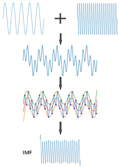
Figure 1.
EMD decomposition flow chart.
Through the above steps, the original signal x(t) can be decomposed into a series of IMFs and the linear superposition of the aftershocks under the EMD method:
After the EMD decomposes each IMF component of the signal, the original signal can be obtained through the superposition and reconstruction of the IMF components.
2.1.2. Advantages of the EMD Method in Analyzing the Radar Emitter Signal
- Basis of principal component analysis
From the introduction of EMD theory, it can be seen that the purpose of EMD is to extract the scale components of the original signal continuously from a high frequency to a low frequency. Then, the decomposed IMF can be arranged according to the frequency from high to low. Thus, the component with the highest frequency is first obtained; then, the sub-high frequency is obtained, and, lastly, a residual component with a very low frequency is obtained. For the signal being constantly decomposed, the high-frequency component with high energy always represents the main characteristics of the original signal and is the most important component. Therefore, the EMD method is a new principal component analysis method that extracts the main component of the signal first and then extracts other low-frequency components.
- 2.
- Adaptive time–frequency analysis
The basic concept of the EMD method is to decompose the signal into a combination of multiple groups of single component signal IMFs. Indeed, the EMD method is equivalent to defining a set of generalized basis functions with adaptive decomposition characteristics. From the perspective of the traditional definition of basis functions, the adaptive generalized basis defined by EMD is innovative in the field of signal processing. Such a basis function is not predetermined or given in advance but depends on the signal itself and is only related to the essential characteristics of the signal, which can be adaptively changed according to the characteristics of the signal in the decomposition process. Therefore, the EMD method has the characteristics of adaptive time–frequency analysis.
- 3.
- Subtle characterization of the signal
The EMD method can obtain the instantaneous frequency of a single component signal by self-adaptively stripping different frequency components of the signal, emphasizing the local instantaneous characteristics of the signal, and completely avoiding the phenomenon in traditional Fourier transform where the known frequency components are used to fit the original sequence and produce false frequency harmonics. The EMD method decomposes the signal into a finite combination of single IMF component signals and defines the physical entity of the instantaneous frequency of the signal. EMD definitions are completely different from the frequency definitions of traditional time–frequency analysis methods. Therefore, the EMD method has a good analysis effect on time-varying, nonlinear, and non-stationary signals, and offers effective characterization capabilities for local transient characteristics.
- 4.
- Increase the sample length
Radar emitter signals are generally composed of many pulses with short durations. Even if IF sampling has a high sampling rate, there will still not be enough data points for traditional feature extraction (such as bispectral feature extraction, HHT, etc.). Multiple IMF components can be obtained through EMD signal decomposition, and a long sequence of signals can be obtained by splicing each IMF. On this basis, secondary feature extraction can be carried out. In this way, the robustness of the neural network can be increased, and the convergence of the network will not be negatively impacted because the signal length is too short.
2.2. Bispectral Characteristics
High-order spectrum analysis is widely used in signal processing. In theory, a high-order spectrum can completely suppress any Gaussian noise and symmetrically distributed non-Gaussian noise [19]. Moreover, high-order spectrum analysis can retain signal amplitude and phase information and is independent of time. Therefore, high-order spectrum analysis has become the mainstream feature extraction method [20]. The third-order spectrum is the simplest high-order spectrum and is also known as the bispectrum. Though the bispectral processing method is relatively simple, it can describe the nonlinear characteristics of the signal. The characteristic function of the k-dimensional random vector is defined as:
among them, . Correspondingly, the second characteristic function of the random vector x is defined as:
The k-th order cumulant of random vector x is the k-th order derivative of its second characteristic function (or cumulant generating function) at the origin). Define the k-order cumulant as:
If the high-order cumulant is absolutely summable, the k-order cumulant spectrum is defined as:
The cumulant higher than the second order is called the high-order cumulant, the multi-dimensional Fourier transform is called the multi-spectrum, and the bispectrum is the third-order spectrum, which is defined as follows:
Compared to the power spectrum, the bispectrum can provide phase information and is widely used. Due to the symmetry of bispectral features, we can reduce the two-dimensional bispectral features to one-dimensional ones based on the symmetry of the features. Common methods include the axial slicing method and the integral method. In the axial slicing method, two-dimensional data are projected onto the axis by selecting the symmetrical axis of bispectral features to rapidly reduce the feature dimension. The integral method involves selecting a symmetrical integral path to integrate the two-dimensional bispectral features along the path, so as to reduce the feature dimension. Integrating the bispectrum is the best way to reduce the characteristic dimension of the two-dimensional bispectrum. According to the different integration paths, the bispectrum can be divided into the axial integral bispectrum (RIB), radial integral bispectrum (AIB), rectangular integral bispectrum (SIB), and circumferential integral bispectrum (CIB). RIB and AIB are symmetrical integral paths, while SIB and CIB are asymmetrical integral paths. The integral path of each integrating bispectrum is shown in Figure 2b.
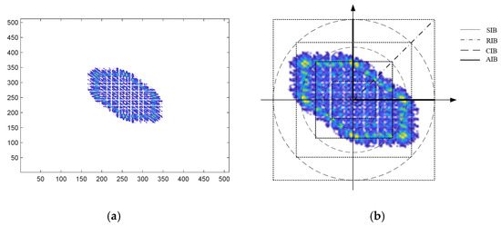
Figure 2.
(a) Two-dimensional bispectral features are obtained by bispectral transformation of the signal; (b) four different integral paths for the dimensionality reduction of two-dimensional bispectral features.
2.3. LeNet—Neural Networks
The design inspiration for CNN comes from the perception of external objects by the visual cortex of the human brain. The human eye transmits the perceived external objects to the brain in the form of images. The brain then abstracts these images layer by layer and extracts the high-dimensional features, such as edges and corners, to make accurate judgments. The CNN was originally designed to solve problems such as image recognition [21]. However, CNN’s current application is not limited to images and videos but also for time series signals such as audio signals and textual data. The simple CNN model structure is shown in Figure 3 below.
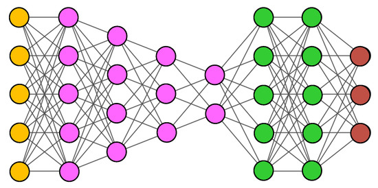
Figure 3.
Schematic diagram of the CNN neural network structure model.
One early SEI strategy based on machine learning is to extract the features of the signals first and then classify the extracted features using various deep learning algorithms, as shown in Figure 4. However, feature extraction algorithms that rely solely on manual selection have limitations. Features automatically extracted by CNN can also achieve better results. CNN does not need to separate the two processes of feature extraction and classification training but instead automatically extracts the most effective features during training. As a deep learning architecture, one appeal of CNN is its ability to reduce the requirements of data preprocessing and avoid complex feature engineering, which can reduce the large amount of repetitive and cumbersome data preprocessing work that must be done when using traditional algorithms such as SVM.
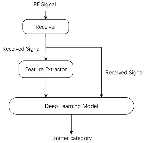
Figure 4.
SEI processing flow based on machine learning.
Figure 5 shows the classical LeNet5 neural network [22,23,24], whose structure consists of an INPUT layer, a convolutional layer (C1), a pooling layer (S2), a convolutional layer (C3), a pooling layer (S4), a convolutional layer (C5), a full-connection layer (F6), and an output layer. In LeNet networks, the nonlinear activation function is performed only once and is not always followed by a nonlinear activation function after each pooling. This process can be seen in the following chart:
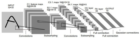
Figure 5.
Two-dimensional LeNet5 neural network.
The LeNet neural network shown in Figure 5 above has a two-dimensional structure, and the input data are two-dimensional image data. To adapt to the recognition and classification of signals in this paper, we transform this network into a one-dimensional LeNet neural network. Specific improvements are described in Section 3.3 below.
3. Experiments and Results
3.1. Experimental Data Processing
The data set used in this experiment is real data of 10 navigation radars with the same model, and the sampling rate is five times the carrier frequency of the radar pulse. Due to the short duration of the radar pulse signal, even with a high sampling rate, only a small number of time–frequency signal points can be collected within a pulse time slot. Due to the small amount of data, it becomes difficult to identify the radar emitter, and some feature extraction methods that require considerable data are no longer applicable. In view of this short radar signal, the present study decomposes each pulse signal by sampling the EMD method to obtain different IMF components. By splitting these IMF components, the bispectral features were used for secondary feature extraction to extract the features of each frequency band of the signal and grow the data to adapt to the one-dimensional LeNet neural network. The specific operation process is shown in Figure 6 below.
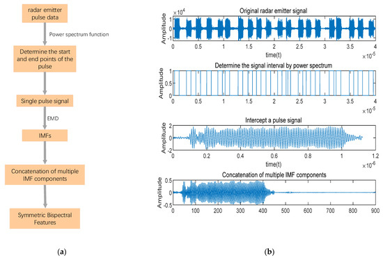
Figure 6.
(a) Signal processing flow chart; (b) the change of the corresponding signal in the signal processing process.
As shown in Figure 6, the starting point and ending point of the radar signal are first determined by the power spectrum. When a signal is sent, the power spectrum will have an obvious peak value. Then, each pulse of the radar signal is intercepted as a sample. Due to the short pulse duration, the interception of each pulse involves only 450 time domain signal points. This factor means that the long time-domain signal transform feature extraction method is no longer applicable and will lead to the extraction of features that are not very stable (e.g., through the double spectrum feature extraction algorithm and the need for feature extraction using the Fourier transform method). Through the method of EMD decomposition, normalized signals are decomposed into several signals of different frequency bands to reflect the characteristics of different frequencies. For example, the high-frequency component with high energy can represent the main characteristics of the original signal, and the low-frequency component can represent the distortion characteristics of the transmitter’s modulator.
As shown in Figure 7, after the five IMF components are joined together, and the axial integral bispectral features of the signals are extracted, the maximum recognition accuracy can be achieved by inputting a two-dimensional LeNet neural network. For this purpose, we take the first five IMF components and concatenate them by row to increase the data for each pulse. The two-dimensional bispectral features are then reduced to one dimension by symmetry, and four signal features representing EMD-AIB, EMD-SIB, EMD-CIB, and EMD-RIB are obtained. By inputting the extracted features into the neural network classifier, we can individually recognize different radiation sources.
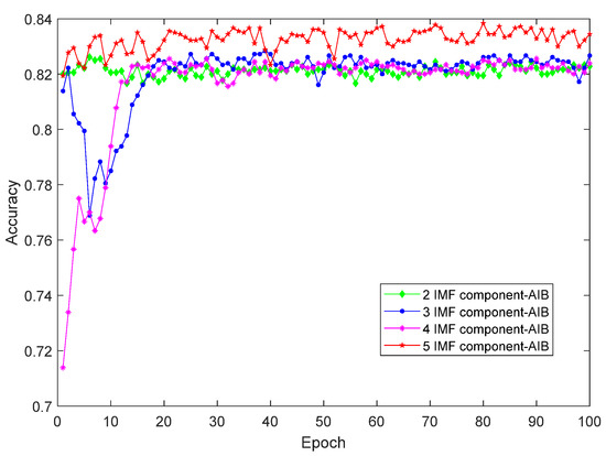
Figure 7.
Influence of splicing different IMF components on the experimental results.
3.2. Influence of Different Neural Networks on the Experimental Results
CNN has three important characteristics: a local receptive field of view, weight sharing, and down sampling. Local receptive field of view: During the convolution operation, the convolution window can find the part that overlaps with the input x(t). Weight sharing: The weight of the convolution window or the pooling window does not change during the convolution operation or pooling operation. Downsampling/desampling: The amount of data can be changed by pooling. The random combination of convolution and pooling endows CNN with great flexibility, yielding many classic networks, such as VGGnet, Google Inception Net, Resnet, Densnet, and LeNet.
In the present study, we employed the EMD-AIB processing method as the feature of our input neural network and used the above neural network to classify and recognize the features. The network parameters follow their original settings, and the classification results are shown in Figure 8.
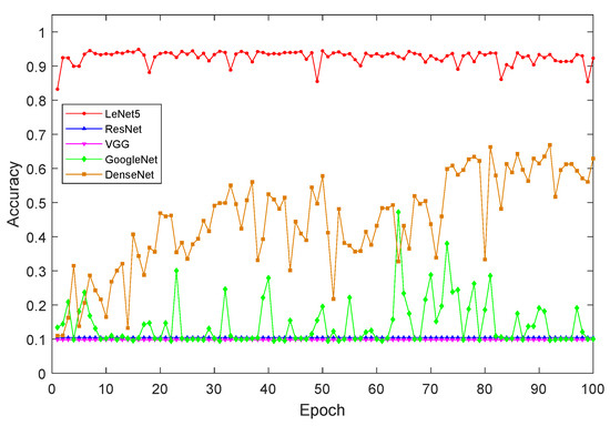
Figure 8.
The relationship between the recognition accuracy of 10 radar emitter sources by different neural networks and their training times.
It can be seen from Figure 8 that LeNet has the best ability to identify the features of the 10 radar emitters, with an average accuracy rate of more than 90%. The Densnet neural network and Googlenet neural network have the ability to distinguish 10 radar emitter sources, but their network training processes are long, and their convergence performance is not as good as that of LeNet. The VGG neural network and Resnet neural network cannot classify the 10 radar emitters. Therefore, the LeNet neural network is more suitable for individual radar emitter identification tasks.
3.3. Parameter Optimization of One-Dimensional LeNet Network
According to the above results for the recognition of EMD-AIB features by different neural networks, it can be seen that the one-dimensional LeNet network has the highest recognition accuracy, is the most sensitive to extracted features, and offers good convergence performance. Therefore, in this paper, we transform the LeNet network into a one-dimensional network that is more suitable for our one-dimensional signal.
First, we change the sizes of the convolution kernels and transform the original two-dimensional convolution kernels into one dimension, in combination with different optimizers, to determine the optimal size of the convolution kernels; the experimental results are shown in Figure 9. We experimentally showed that, for a convolution kernel size of 1 × 5, the Nadam optimization algorithm provides the highest classification accuracy for 10 radar signals. Therefore, the convolution kernel size chosen for our improved one-dimensional LeNet network is 1 × 5, and the optimizer is the Nadam optimizer.
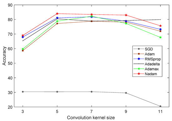
Figure 9.
The Influence of convolution kernels and optimizers of different sizes on the recognition accuracy rate.
After the parameters of the network were determined, the network structure was adjusted to further optimize the performance of the network by changing the number of layers in the convolutional layer and the full connection layer. The experimental results are shown in Figure 10.
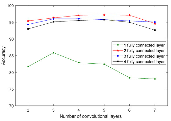
Figure 10.
The influence of the number of convolution layers and the number of full connection layers on the recognition accuracy.
Figure 10 shows that for a convolution kernel size of 1 × 5, the best optimizer is the Nadam optimizer, the number of convolution layers is four, and the number of full connection layers is two. Here, the EMD-AIB feature extraction algorithm is adopted for the data of the 10 radar emitter sources to achieve the best recognition performance through the improved one-dimensional LeNet network. The improved LeNet network structure is shown in Figure 11.
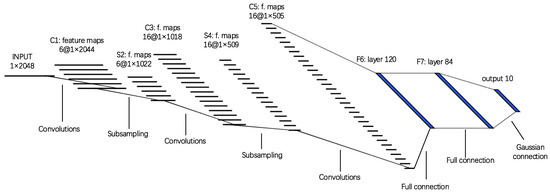
Figure 11.
Adaption to the improved one-dimensional LeNet network.
The improved one-dimensional LeNet network is used to identify the 10 radar pulse signals. The recognition accuracy of the network and the loss curve are shown in Figure 12 below.
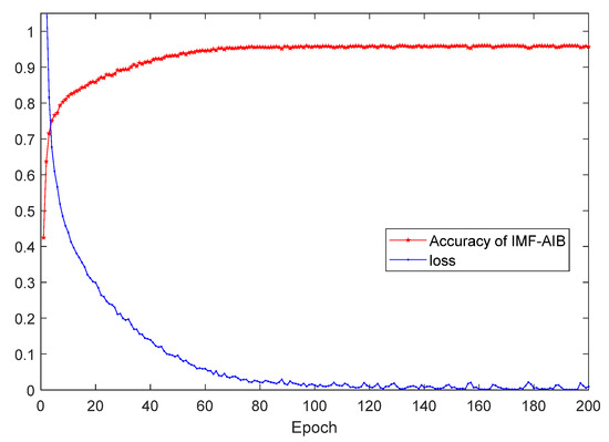
Figure 12.
This figure shows the identification results for the 10 radar emitter sources using the improved one-dimensional LeNet neural network. Relational diagram of the loss curve for recognition accuracy and training times.
The confusion matrix can help us quickly visualize the recognition of 10 radar radiation sources. The confusion matrix is shown in Figure 13 below.
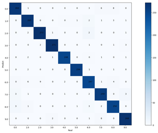
Figure 13.
This figure shows the identification results for the 10 radar emitter sources using the improved one-dimensional LeNet neural network. confusion matrix of 10 radar emitters.
Figure 12 shows that when the Epoch exceeds 50 times, the one-dimensional LeNet network tends to be stable, and the identification accuracy of the improved one-dimensional LeNet network for 10 radar emitter sources exceeds 95%. Compared with the original two-dimensional LeNet5 network, the recognition accuracy is greatly improved, and the convergence of the network is obviously improved.
3.4. The Influence of Different Artificial Features on Recognition Accuracy
3.4.1. Bispectrum Algorithm Used as Fingerprint Characteristics
In order to verify the recognition ability of EMD plus bispectral extraction of fingerprint features of radiation sources proposed in this paper, we directly extracted the bispectral features of radar pulse signals. Figure 14 presents the results for the experimental comparison between EMD and the bispectral extraction of the fingerprint features of radiation sources.
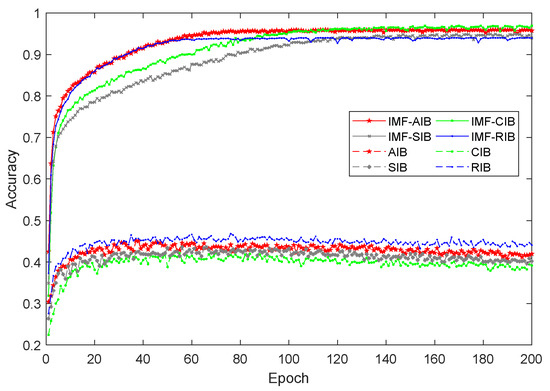
Figure 14.
Recognition ability of one-dimensional LeNet networks with different feature extraction algorithms.
Direct feature extraction from radar pulse signals will result in unstable bispectral extraction results due to an insufficient data volume and large intra-class differences. Through EMD decomposition, the amount of data will be significantly increased. In addition, EMD extracts different frequency components of the signal and the main frequency band, ignores some stray interference, and then extracts secondary features through the bispectrum, which can reduce the sensitivity of the bispectrum features to the frequency. This factor can increase the robustness of the present method against frequency-unstable emitters.
3.4.2. Radar Pulse Parameters Used as Fingerprint Characteristics
According to the real waveform of the pulse signal, the various parameters of the rectangular pulse can be defined as follows [25]:
- Pulse amplitude refers to the difference between the maximum and minimum pulse values, represented as A in Figure 15.
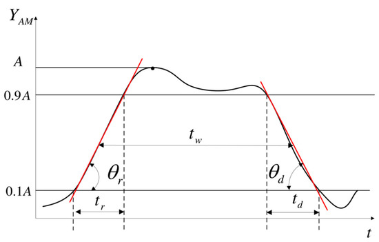 Figure 15. Schematic diagram of radar pulse parameter definitions.
 - Pulse rise time refers to the time required for 10% of the pulse amplitude to rise to 90% of the pulse amplitude, which is in Figure 15.
- Pulse drop time refers to the time required for 90% of the pulse amplitude to drop to 10% of the pulse amplitude, i.e., in Figure 15.
- Pulse width refers to the time interval between two points corresponding to 50% of the pulse amplitude, which is in Figure 15.
We analyzed each radar pulse and extracted the pulse amplitude, pulse rise time, pulse fall time, and pulse width, which were combined into the feature vector and classified by the SVM classifier. The obtained results are shown in Table 1.

Table 1.
Comparison table of the accuracy results for the EMD-AIB identification method and the method using pulse parameters.
Figure 16 shows that the pulse widths sent by different emitters differ to a certain extent while the amplitude has great volatility. However, the insufficient feature dimensions limit recognition accuracy. When we need to extract more parameters from the pulse, more complex calculations and higher accuracy are required, which limits the applications for this type of method.
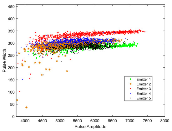
Figure 16.
Five different radar signals, their pulse amplitudes, and their pulse widths: two-dimensional visualization.
3.4.3. Skewness and Kurtosis Were Used as Fingerprint Characteristics
In [12], the authors used EMD, ITD, and VMD to decompose signals. The skewness and kurtosis were extracted from each decomposed IMF component signal to characterize the non-Gaussian characteristics of the signal. The support vector machine (SVM) or back propagation (BP) neural network was then used to fuse the features extracted from multiple distortion receivers, and the unknown radiation source was identified.
Kurtosis and skewness are statistics that describe the non-Gaussian characteristics of a signal. Kurtosis describes the overall distribution of all values in the form of statistic for the steep–slow degree. These statistics must then be compared with the normal distribution. A kurtosis of 0 indicates that the overall data distribution and normal distribution of the steep–slow degree are the same; the greater the absolute value of kurtosis according to the distribution form of the steep–slow degree, the greater the difference degree of normal distribution. Skewness is similar to kurtosis and is also a type of statistic used to describe the data distribution form. Skewness describes the symmetry of the distribution of a certain population value. Skewness of 0 means that the data distribution form has the same degree of skewness as the normal distribution; the greater the absolute value of skewness, the greater the degree of skewness.
For the signal , skewness S and kurtosis K are defined as follows:
where and represent the mean and standard deviation of signal , respectively. We then calculate the EMD components of 10 radar pulse signals followed by the skewness and kurtosis characteristics of each component. The characteristic vector can thus be obtained. We compared these outputs with the results of the method outlined in the present study. The experimental results are illustrated in Figure 17. It can be seen from the figure that the SEI method of literature [12] does not have a very good effect on this data set.
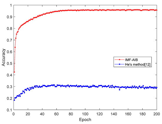
Figure 17.
The relationship between the training times and accuracy of the method presented in this paper and the method proposed in [12].
3.5. Different Types of Radiation Source Identification Ability Verification
To verify the recognition ability of this algorithm for different types of radiation sources, we selected 10 real radar emitter signals, 10 real data emitter signals, and 5 real ultra-shortwave communication emitter signals for experimental verification. The identification results are shown in Table 2.
Table 2.
The recognition rate of the method in this paper under different radiation sources.
Radar emitter signals are pulse signals, and each radar signal is collected with 1000 pulses. Each pulse features 450 time domain points. EMD-AIB is used to extract the fingerprint features that can represent individual emitter sources. Using the one-dimensional LeNet neural network, the classification and recognition accuracy of the 10 radar pulse signals was found to be 96.4%. The 10 data emitter sources employ FSK modulation, with a carrier frequency of 150 kHz and a five-times over-sampling rate. Using the method in this paper, the classification and recognition accuracy of the 10 data emitter sources was found to be 98.9%. Five ultra-shortwave communication radiation sources with FM modulation were classified and identified by the method presented in this paper, and the recognition accuracy was determined to be 88.93%. From the above analysis, it can be seen that a combination of the feature extraction algorithm and the one-dimensional LeNet neural network proposed in this paper offers good recognition accuracy for radar transmitters, data transmitters, and communication transmitters alongside some adaptability to different circumstances.
4. Conclusions
Using the method proposed in this paper, EMD was able to decompose the signal into the superposition of several different frequency components. By selecting a combination of the first several important IMF components, we not only increased the data length but also increased the frequency characteristics of the signal. By employing the secondary feature extraction of bispectral transformation, the fingerprint features of the signal frequency, phase, and amplitude were obtained, thereby enhancing the ability to characterize the bispectral fingerprints of radiation sources. According to the symmetry of the bispectrum, the two-dimensional features were reduced by one dimension and input into the improved one-dimensional LeNet network to achieve the individual classification and recognition of different radiation sources. The classification and recognition accuracy of the proposed method was 96.4% for 10 real radar pulse signals, 98.8% for 10 real data emitter signals, and 88.93% for 5 ultra-shortwave communication radiation signals. The experimental results show that the proposed method has a high recognition accuracy and can adapt to a variety of different radiation sources.
Author Contributions
Conceptualization, Y.C. and Z.-L.W.; methodology, Y.C.; software, Y.C.; validation, Z.-L.W. and Y.-K.L.; formal analysis, Z.-L.W.; investigation, Z.-L.W.; resources, Y.-K.L.; data curation, Z.-L.W.; writing—original draft preparation, Z.-L.W.; writing—review and editing, Z.-L.W.; visualization, Y.C.; supervision, Y.-K.L.; project administration, Y.-K.L.; funding acquisition, Y.-K.L. All authors have read and agreed to the published version of the manuscript.
Funding
This research was funded by National Natural Science Foundation of China, grant number 62071479.
Institutional Review Board Statement
Did not involve humans or animals.
Informed Consent Statement
Not applicable.
Data Availability Statement
Not applicable.
Conflicts of Interest
The authors declare no conflict of interest.
References
- Tang, Z.L. A Study of Nonlinear Method for Specific Communications Emitter Identification. Ph.D. Thesis, Xidian University, Xian, China, 2013. [Google Scholar]
- Jia, Y. The Research on Communication Emitters Identification Technology. Ph.D. Thesis, University of Electronic Science and Technology of China, Chengdu, China, 2017. [Google Scholar]
- Xing, Y.; Hu, A.; Zhang, J.; Yu, J.; Li, G.; Wang, T. Design of a Robust Radio-Frequency Fingerprint Identification Scheme for Multimode LFM Radar. IEEE Internet Things J. 2020, 7, 10581–10593. [Google Scholar] [CrossRef]
- Reising, D.R.; Temple, M.A.; Mendenhall, M.J. Improved wireless security for gmsk-based devices using RF fingerprints. Int. J. Electron. Secur. Digit. Forensics 2010, 3, 41–59. [Google Scholar] [CrossRef]
- Williams, M.D.; Temple, M.A.; Reising, D.R. Augmenting bit-level network security using physical layer RF-DNA fingerprinting. In Proceedings of the IEEE Globecom, Miami, FL, USA, 8–10 December 2010; pp. 1–6. [Google Scholar]
- Williams, M.D.; Munns, S.A.; Temple, M.A.; Mendenhall, M.J. RF-DNA fingerprinting for airport WiMax communications security. In Proceedings of the IEEE International Conference Network and System Security, Melbourne, Australia, 1–3 September 2010; pp. 32–39. [Google Scholar]
- Dubendorfer, C.; Ramsey, B.; Temple, M. ZigBee Device Verification for Securing Industrial Control and Building Automation Systems; Critical Infrastructure Protection; Springer: Berlin/Heidelberg, Germany, 2013; pp. 47–62. [Google Scholar]
- Dubendorfer, C.K.; Ramsey, B.W.; Temple, M.A. An RF-DNA verification process for ZigBee networks. In Proceedings of the IEEE Military Communication Conference, Orlando, FL, USA, 29 October–1 November 2012; pp. 1–6. [Google Scholar]
- Lin, Y.; Jia, J.; Wang, S.; Ge, B.; Mao, S. Wireless Device Identification Based on Radio Frequency Fingerprint Features. In Proceedings of the ICC 2020—2020 IEEE International Conference on Communications (ICC), Dublin, Ireland, 7–11 June 2020. [Google Scholar]
- Wang, L. On Methods for Specific Radar Emitter Identification. Ph.D. Thesis, Xidian University, Xian, China, 2011. [Google Scholar]
- Huang, N.E.; Shen, Z.; Long, S.R. The empirical mode decomposition and the Hilbert spectrum for nonlinear and non-stationary-ime series analysis. Proc. R. Soc. A 1998, 454, 903–995. [Google Scholar] [CrossRef]
- He, B.; Wang, F. Cooperative Specific Emitter Identification via Multiple Distorted Receivers. IEEE Trans. Inf. Forensics Secur. 2020, 15, 3791–3806. [Google Scholar] [CrossRef]
- Klein, R.W.; Temple, M.A.; Mendenhall, M.J. Application of wavelet based RF fingerprinting to enhance wireless network security. Commun. Netw. 2009, 11, 544–555. [Google Scholar] [CrossRef]
- Klein, R.W.; Temple, M.A.; Mendenhall, M.J. Application of wavelet denoising to improve OFDM-based signal detection and classification. Secur. Commun. Netw. 2010, 3, 71–82. [Google Scholar] [CrossRef]
- Wambacq, P.; Sansen, W. Distortion Analysis of Analog Integrated Circuits; Kluwer Academic Publishers: Boston, MA, USA, 1998. [Google Scholar]
- Lu, J.; Qin, X.; Xu, X.; Lei, Y. Identification of Multiple-Antenna Emitters Using Power Amplifier Nonlinearity. In Proceedings of the 2020 5th International Conference on Computer and Communication Systems (ICCCS), Shanghai, China, 15–18 May 2020. [Google Scholar]
- Jian, C.; Duan, T. Nonlinear feature extraction of power amplifiers in multipath. In Proceedings of the 2015 4th International Conference on Computer Science and Network Technology (ICCSNT), Harbin, China, 19–20 December 2015. [Google Scholar]
- Shi, F.; Chen, Z.; Cheng, X. Behavior Modeling and Individual Recognition of Sonar Transmitter for Secure Communication in UASNs. IEEE Access 2019, 8, 2447–2454. [Google Scholar] [CrossRef]
- Liang, B.; Iwnicki, S.D.; Zhao, Y. Application of power spectrum, cepstrum, higher order spectrum and neural network analyses for induction motor fault diagnosis. Mech. Syst. Signal Process. 2013, 39, 342–360. [Google Scholar] [CrossRef]
- Zhang, X.D.; Shi, Y.; Bao, Z. A new feature vector using selected bispectra for signal classification with application in radar target recognition. IEEE Trans. Signal Process. 2001, 49, 1875–1885. [Google Scholar] [CrossRef]
- Riaz, H.; Park, J.; Choi, H.; Kim, H.; Kim, J. Deep and Densely Connected Networks for Classification of Diabetic Retinopathy. Diagnostics 2020, 10, 24. [Google Scholar] [CrossRef] [PubMed] [Green Version]
- Lecun, Y.; Bottou, L.; Bengio, Y.; Haffner, P. Gradient-based learning applied to document recognition. Proc. IEEE 1998, 86, 2278–2324. [Google Scholar] [CrossRef] [Green Version]
- Shao, X.; Nie, X.; Zhao, X.; Zheng, R.; Guo, D. Gait Recognition based on Improved LeNet Network. In Proceedings of the 2020 IEEE 4th Information Technology, Networking, Electronic and Automation Control Conference (ITNEC), Chongqing, China, 12–14 June 2020; pp. 1534–1538. [Google Scholar] [CrossRef]
- Li, S.; Xie, G.; Ji, W.; Hei, X.; Chen, W. Fault Diagnosis of Rolling Bearing Based on Improved LeNet-5 CNN. In Proceedings of the 2020 IEEE 9th Data Driven Control and Learning Systems Conference (DDCLS), Liuzhou, China, 20–22 November 2020; pp. 117–122. [Google Scholar] [CrossRef]
- Fan, Y. The Feature Ectraction of Rader Source and Rader Individual Idetification. Master’s Thesis, Xidian University, Xian, China, 2017. [Google Scholar]
Publisher’s Note: MDPI stays neutral with regard to jurisdictional claims in published maps and institutional affiliations. |
© 2021 by the authors. Licensee MDPI, Basel, Switzerland. This article is an open access article distributed under the terms and conditions of the Creative Commons Attribution (CC BY) license (https://creativecommons.org/licenses/by/4.0/).