Evolving Hybrid Cascade Neural Network Genetic Algorithm Space–Time Forecasting

Abstract

Design: At the heart of time series forecasting, if nonlinear and nonstationary data are analyzed using traditional time series, the results will be biased. At the same time, if just using machine learning without any consideration given to input from traditional time series, not much information can be obtained from the results because the machine learning model is a black box. Purpose: In order to better study time series forecasting, we extend the combination of traditional time series and machine learning and propose a hybrid cascade neural network considering a metaheuristic optimization genetic algorithm in space–time forecasting. Finding: To further show the utility of the cascade neural network genetic algorithm, we use various scenarios for training and testing while also extending simulations by considering the activation functions SoftMax, radbas, logsig, and tribas on space–time forecasting of pollution data. During the simulation, we perform numerical metric evaluations using the root-mean-square error (RMSE), mean absolute error (MAE), and symmetric mean absolute percentage error (sMAPE) to demonstrate that our models provide high accuracy and speed up time-lapse computing.

1. Introduction

Pollution describes the appearance and retention of the regular circulation of material, fine particles, biomaterial, and energy, or a deterioration technique or atmospheric change, which also has or may have significantly negative effects on human beings or the natural environment. Air pollutants are exhaust gases, particulate matter compounds, solid particulate matter, and other substances that emanate into the air, threatening the health of the community and damaging the environment. Air pollutants can be classified into smog and soot, pollution from contaminated air, greenhouse gas emissions, pollen, and mold.

PM refers to particulate matter, also known as particulate emissions. PM comprises aggregated rigid particles and atmospheric fluid droplets. Some are large enough or visible enough to be seen with the naked eye, and others are so small that they can only be seen with electron microscopes. PM₁₀ and PM_2.5 are some classes of these particulate pollutants [1,2,3,4]. Let us consider a hair: the mean diameter of a single human hair is approximately 70 micrometers. This is roughly 28 times the diameter of PM_2.5. The diameter of particulate matter in PM₁₀ is 10 micrometers or below. Similarly, PM_2.5 is normally particles of diameter 2.5 micrometers or below. Both PM₁₀ and PM_2.5 are inhalable. We can thus imagine how tiny 2.5 and 10 micrometers are.

PM can be made up of various chemicals, including sulfur dioxide (SO₂) and nitrogen oxides, originating in PM (NOx) [5,6,7]. All this can be found as a product of building materials, farms, explosions, power stations, industry, and vehicles. PM is seriously damaging, as described above, as it may be opaque and small enough to be inhaled into the lungs or even into the circulation. Therefore, PM contamination affects the cardiovascular system and can cause fatal illnesses such as cardiovascular diseases, erratic heartbeat, and worsening asthma [8,9,10].

The estimation of future air pollution is an important task because it can be used to manage risk. The Artificial Neural Network (ANN) is the most frequently used among many data-driven applications and is a modern method and an effective paradigm for predicting and forecasting variables in the management of contamination risk due to intrinsic contaminant source uncertainties using quality data [11,12]. ANNs were inspired by the human brain’s biochemical neural networks. McCulloch and Pitts in (1943) [13] initially developed a mathematically dependent model and referred to it as a threshold logic computing model for neural networks [14,15,16,17,18,19].

The neurons are important in the neural network’s operating condition, they are very connected and share signals with one another, whether it is a neuron or node. Every layer consists of one or more simple elements called neurons. As the input data are transferred to the input layer, they bind with the weight and are nonlinearized by the activation function; the process of being sent to the next neuron is replicated before the final outcome is achieved. Each new neuron consists of one weight and one activation function [20,21]. The connectivity of neurons is handled by utilizing established inputs and outputs and is seen in an organized way in the ANN. The training phase is represented as a trial-and-error process to select the number of neurons [22,23]. The intensity of these interconnections is adapted to the known pattern using an error convergence technique. In this article, a cascade neural network procedure based on the genetic algorithm is developed for space–time forecasting data. This article is organized as follows: In Section 2, we review the training using the cascade neural network and employ a genetic algorithm. The performance is examined in Section 3 via simulation studies and analysis of four benchmark real datasets of air pollution data. Finally, Section 4 presents our conclusions.

2. Methods

2.1. Cascade Neural Network

The neural network’s environment is uncertain. It is presumed that the teacher and the neural network are linked to an environmental testing vector, as an example. Because of the integrated experience, the teacher is capable of responding to this training vector in the algorithm. In fact, the appropriate outcome is the optimal response of the neural network. The key property of a neural network is the network’s capacity to improve performance by learning from its experience [24]. Based on how well the neural networks operate, the networks are divided into supervised learning networks and unsupervised learning networks, otherwise termed teacher learning and teacher-free learning. Structurally, we may think of the teacher as having information about the environment, portrayed by a variety of samples of input and output [25,26].

The network parameters are managed according to the cumulative effect of the training vector, mostly with error signals. Meanwhile, each error signal should be specified as the gap between the requested response and the network’s actual response. This modification is made step by step in order to rapidly mimic the teacher in the neural network, with the emulation in any mathematical context assumed to be ideal. This transfers awareness of the teacher’s setting to the neural network as thoroughly as possible by preparation [27]. If this is achieved, then we can dispense with the teacher and encourage the neural network to deal entirely with the environment. Throughout the supervised NN model, input vectors and suitable target vectors are used to update the parameters; before a function can be approximated, input features should be tied to specific output vectors and the information that can be processed should be properly identified [28,29].

The most famous and typical algorithm for neural network training is the context of an error, the main principle of which is that an error in the hidden neurons is calculated by propagation of the error in the output layer neurons. The traditional backpropagation algorithm uses two input and learning processes. Vectors or patterns are displayed in the input layer in feedforward operation, and each neuron throughout the hidden layer is measured in the activation with one neuron $ne{t}_j.$ The input vector dot product including neuron weight in the hidden layer is represented in Equation (1):

$$ne{t}_j={\displaystyle \sum }_{i=1}^{N_i}{x}_i{w}_{ij}^{I-H}+b_{ij}={\displaystyle \sum }_{i=0}^{N_i}{x}_i{w}_{ij}^{I-H}$$

(1)

where $N_i$ is the input vector dimension, and $i$ and $j$ are neuron indices in the layer input and in the hidden layer, respectively. The weight value between the input vectors and neurons in the hidden layer is $w_{ij}^{I-H}$. The weight value of bias in the hidden layer is $b_{ij}$ and is usually assumed to be $b_{ij}=w_{0j}^{I-0}, x_0=1$. By substituting $ne{t}_j$ into activation function ${\phi }_1, {\theta }_j$ is calculated. In the activation of a single neuron, each neuron in the output layer computes $ne{t}_k$, which is the dot product of ${\theta }_j$ and the neuron weight in the output layer, represented in Equations (2) and (3).

$${\theta }_j={\phi }_1\left(ne{t}_j\right)$$

(2)

$$ne{t}_k={\displaystyle \sum }_{j=1}^{N_H}{\theta }_j{w}_{jk}^{H-0}$$

(3)

In line with this, $N_H$ is the number of neurons in the hidden layer and $k$ is the index of a neuron in the output layer. The weight value of neurons between the hidden layer and output layer is described as $w_{jk}^{H-0}.$ We can substitute $ne{t}_k$ into activation function ${\phi }_2$ to output $y_k$, represented in Equation (4).

$$y_k={\phi }_2\left(ne{t}_k\right)$$

(4)

$$y_k={\phi }_2\left({\displaystyle \sum }_{j=1}^{N_H}{\theta }_j{w}_{jk}^{H-0}\right)$$

(5)

$$y_k={\phi }_2\left({\displaystyle \sum }_{j=0}^{N_H}{w}_{jk}^{H-0}\left({\displaystyle \sum }_{i=0}^{N_i}{x}_j{w}_{ij}^{I-H}\right)\right)$$

(6)

Regarding Equations (4) and (5), the entire collection of weights is updated to ensure that $y_k$ is near the target output value of $t_k$ by propagating the $E_r$ error of the output layer neurons throughout the learning phase. Although a variety of output functions are available to evaluate the error, the squared error is commonly used, represented in Equation (7).

$$E_r={\displaystyle \sum }_{k=1}^{N_0}{\left(t_k-y_k\right)}^2$$

(7)

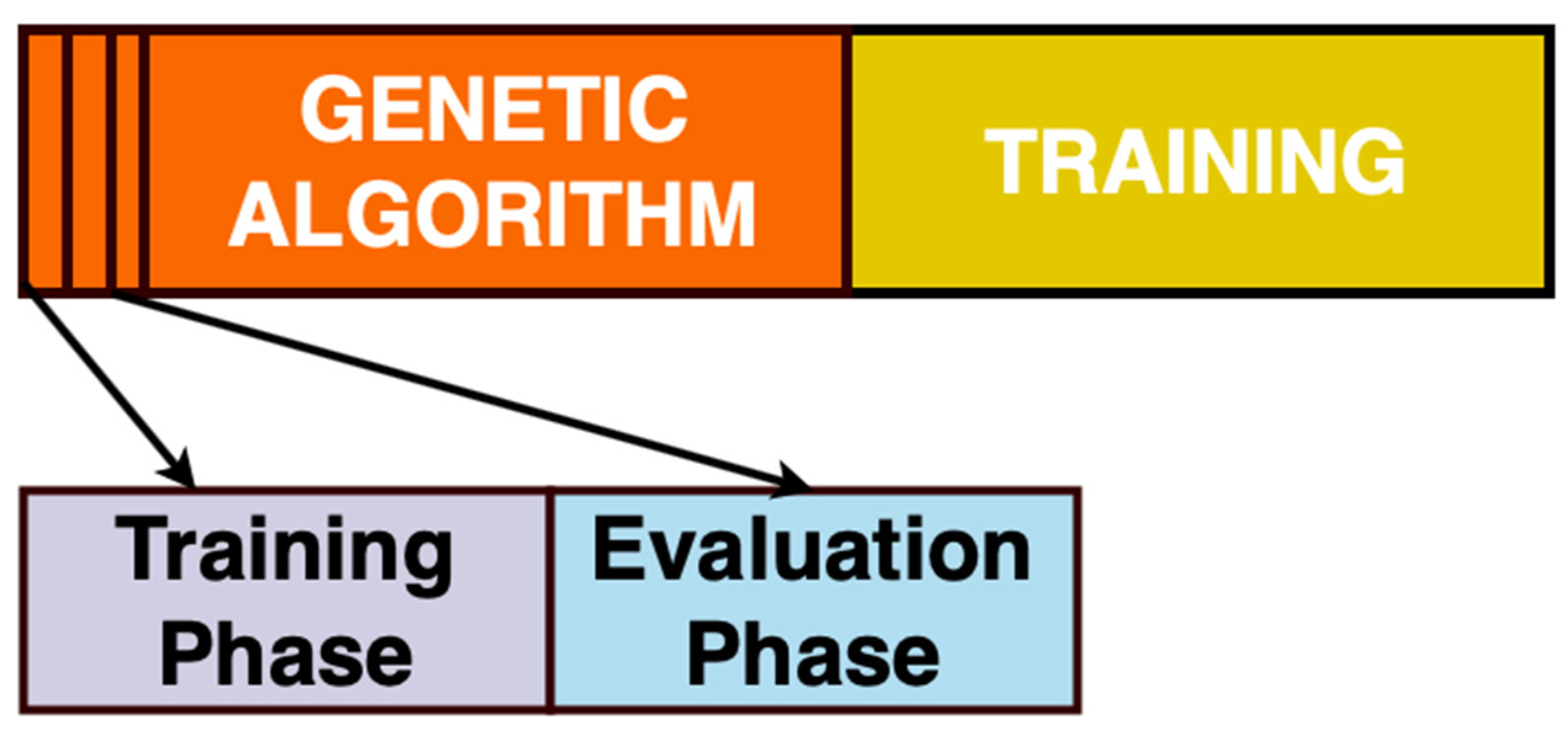
2.2. Genetic Algorithm

Biological variation and its basic processes were clarified by Darwin’s (2002) evolutionary theory [30]. Natural selection is fundamental to what is often referred to as the macroscopic understanding of evolution. In an environment where only a finite number of humans will survive, and given the basic tendency of people to multiply, selection is necessary if people do not have an accelerated population [31,32]. This evolution favors people who bid more successfully for the given resources. In other words, they are better suited or adapted to the climate, recognized as global best survival [33].

Selection on the basis of competition is one of the two pillars of the mechanism of evolution. The other main influence comes as a function of phenotypical differences in the populations. The phenotype is an individual’s physical and behavioral characteristics that assess their fitness in terms of their exposure to the surrounding environment. That individual represents a specific combination of environmental assessment phenotypic characteristics. These characteristics are inherited by the offspring of the individual if evaluated with favor; otherwise, the offspring is discarded. Charles Darwin’s insight was that slight, spontaneous phenotype changes occur across ages [34,35,36].

New combinations of phenotype arise and are assessed by these mutations. That is the fundamental basis of the genetic algorithm: With a population of individuals, constraints on the environment lead to natural selection and survival of the population via roulette wheel selection, which results in an increase in the fitness of the population. A random collection of candidates can be generated [37]. Depending on this fitness, many of the best candidates are selected for the next generation using conjugation to seed the performance as an abstract fitness metric [38]. Cross-over and mutation give rise to a number of new offspring that fight for a position in the next generation on the basis of their fitness with old members of the population, before an organism of adequate efficiency is identified and until a previously determined computational threshold is exceeded [39,40]. In line with this, Algorithm 1 shows the scheme of the genetic algorithm. The scheme coincides with the generate-and-test algorithm type. The fitness function constitutes a heuristic estimate of an optimal solution, and the cross-over, mutation, and selection operators guide the search algorithm. The genetic algorithm has many characteristics that can support in the generating and testing of parents.

Algorithm 1. Scheme of the GA
1:	INITIALIZE population and EVALUATE
2:	while termination condition is not satisfied do
3:	SELECT parents
4:	CROSSOVER pairs of parents
5:	MUTATE the resulting offspring
6:	EVALUATE new candidates
7:	REPLACE individuals for the next generation
8:	end while

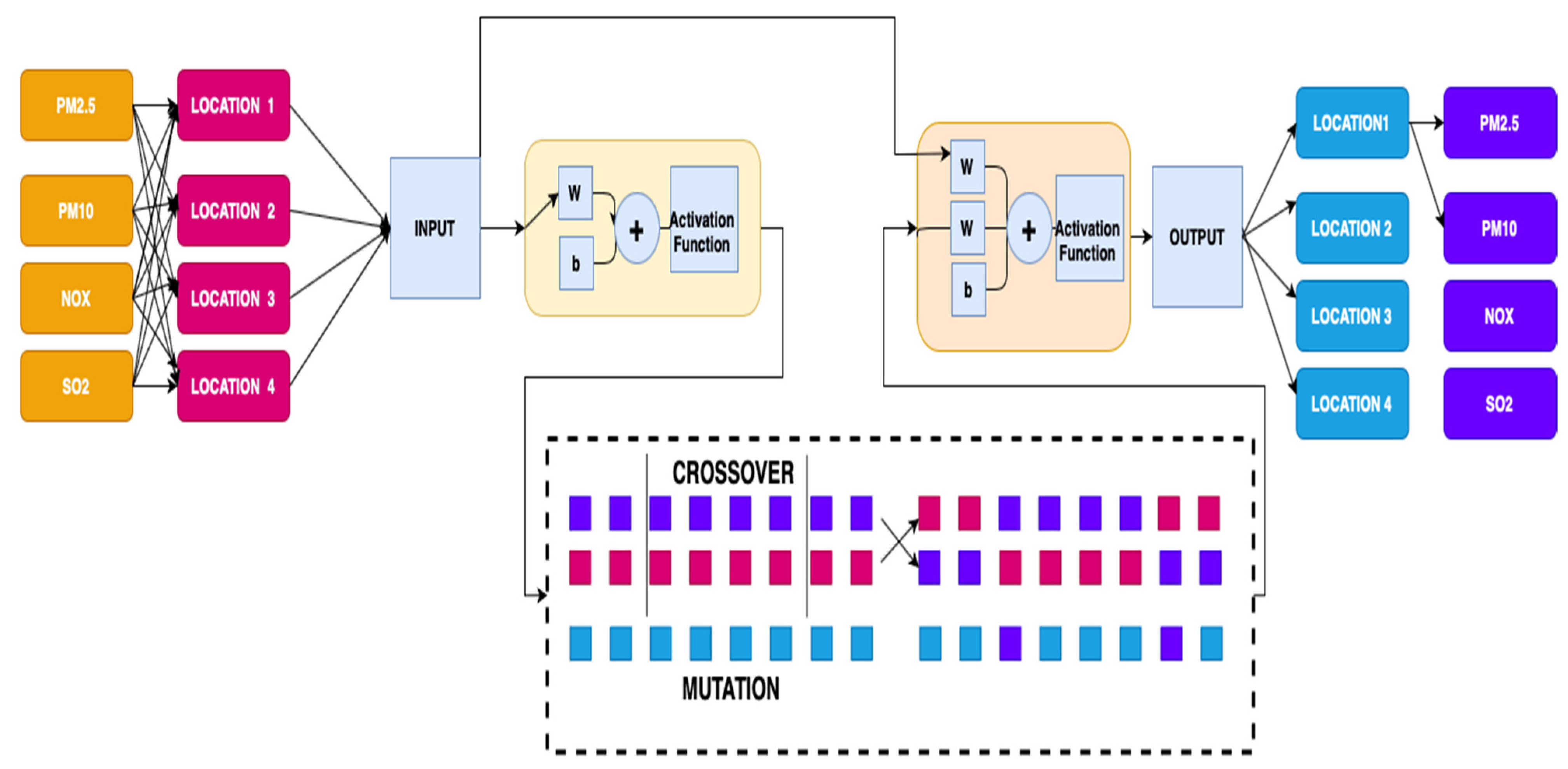
2.3. Cascade Neural Network Genetic Algorithm

Backpropagation training algorithms based on other traditional optimization methods, such as the conjugating gradient and Newton process, have different variants. This same gradient descent approximation, the easiest and among the slowest, usually speeds up the conjugate gradient algorithm, as well as Newton’s method [41,42]. We used genetic algorithms through this study. Each neuron weight between the hidden layer and the output layer should be updated, and the weight of the neurons here between the input and the hidden layer was adjusted [43]. The weight change between some of the hidden and output layers of the neuron is specified in Equation (8) with activation function $\phi \left(x\right)=\frac{1}{x}.$

$$\frac{\partial E_r}{\partial w_{jk}^{H-0}}=\frac{\partial E_r}{\partial ne{t}_k}·\frac{\partial ne{t}_k}{\partial w_{jk}^{H-0}}$$

$$\frac{\partial E_r}{\partial w_{jk}^{H-0}}=-\left(t_k-y_k\right)·{\phi }^2\left(ne{t}_k\right)·{\theta }_j$$

(8)

The weight value of neurons was updated between the input and hidden layer as represented in Equation (9).

$$\frac{\partial E_r}{\partial w_{jk}^{I-H}}=\frac{\partial E_r}{\partial {\theta }_j}·\frac{\partial {\theta }_j}{\partial ne{t}_k}·\frac{\partial ne{t}_k}{\partial w_{jk}^{I-H}}$$

$$\frac{\partial E_r}{\partial w_{jk}^{I-H}}=\left[\frac{1}{2}{\displaystyle \sum }_{k=1}^{N_0}{\left(t_k-y_k\right)}^2\right]·\frac{\partial {\theta }_j}{\partial ne{t}_k}·\frac{\partial ne{t}_k}{\partial w_{jk}^{I-H}}$$

$$\frac{\partial E_r}{\partial w_{jk}^{I-H}}=\left[{\left(t_k-y_k\right)}^2·\frac{\partial y_k}{\partial {\theta }_j}\right]·\frac{\partial {\theta }_j}{\partial ne{t}_k}·\frac{\partial ne{t}_k}{\partial w_{jk}^{I-H}}$$

$$\frac{\partial E_r}{\partial w_{jk}^{I-H}}=\left[{\left(t_k-y_k\right)}^2·\frac{\partial y_k}{\partial ne{t}_k}\frac{\partial ne{t}_k}{\partial {\theta }_j}\right]·\frac{\partial {\theta }_j}{\partial ne{t}_j}·\frac{\partial ne{t}_j}{\partial w_{ij}^{I-H}}$$

$$\frac{\partial E_r}{\partial w_{jk}^{I-H}}=-{\displaystyle \sum }_{k=1}^{N_0}\left[\left(t_k-y_k\right)·{\phi }_2\left(ne{t}_k\right)·w_{jk}^{H-0}\right]·{\phi }_1\left(ne{t}_j\right)·x_i$$

(9)

With backpropagation, the input data are repeatedly presented to the neural network. With each presentation, the output of the neural network is compared to the desired output, and the error is computed. This error is then backpropagated through the neural network and used to adjust the weights such that the error decreases with each iteration; the neural network thus gets closer and closer to producing the desired output, represented in Equation (10).

$$w\left(h+1\right)=w\left(h\right)+∆w\left(h\right)$$

(10)

Algorithm 2 shows the function cascade neural network. However, the context backpropagation of each input datum is continuously shown to the neural network, with every representation comparing the output of the neural network to the requested output and computing the error; these errors provide context to the neural network and are used to update the weights to reduce its error for each iteration, as well as the genetic algorithm, allowing new generation of the neural network.

Algorithm 2. Function Cascade Neural Network
1:	input$n_h, m, o$
2:	setk = 0
3:	calculate Cascade Weighted
4:	k = 0;   for i = 1:nh    for j = 1:m      k = k + 1; Wi1(i,j) = W(k);   end end
5:	calculate weighted input and output
6:	fori = 1:o   for j = 1:m   k = k + 1;   Wi2(i,j) = W(k);   end end
7:	calculate weighted Bias Input
8:	fori = 1:nh   k = k + 1;   Wbi(i,1) = W(k); end
9:	calculate weighted output
10:	fori = 1:o   for j = 1:nh   k = k + 1;   Wo(i,j) = W(k);   end end
11:	calculate weighted Bias Output
12:	fori = 1:o   k = k + 1;   Wbo(i,1) = W(k); end

3. Simulation and Results

3.1. Construction of VAR-Cascade

There exist few guidelines for building a neural network model for time series. One of them considers time series as a nonlinear function of several past observations and random errors. Since air pollution data are known to be nonlinear time series data, we selected this method as a benchmark for forecasting. Equation (11) represents the time series models:

$$y_t=f\left[\left(z_{t-1},z_{t-2},\dots ,z_{t-m}\right), \left(e_{t-1},e_{t-2},\dots , e_{t-n}\right)\right]$$

(11)

where $f$ is a nonlinear function determined by the neural network, $z_t={\left(1-B\right)}^d y_t$, and $d$ represents the order difference. Also, the residuals at time $t$ are defined as $e_t$, and $m$ and $n$ are integers. Equation (12) shows that, initially, the VAR model is fitted in order to generate the residuals $e_t$. A neural network is then used to model the nonlinear and linear relations in excess and the original results [22,44,45].

$$z_t=w_0+{\displaystyle \sum }_{j=1}^Q{w}_j·g\left(w_{0j}+{\displaystyle \sum }_{i=1 }^p{w}_{ij}·z_{t-i}+{\displaystyle \sum }_{i=p+1}^{p+q}{w}_{ij}·e_{t+p-i}\right)+{ϵ}_t$$

(12)

Here, $w_{ij}\left(i=0,1,2,\dots ,p+q,j=1,2,\dots ,Q\right)$ and $w_j\left(j=0,1,2,3,\dots , Q\right)$ are connection weights and $p,q,Q$ are integers that should be determined in the design process of the cascade neural network. The values of $p$ and $q$ are determined by the underlying properties of the data. If the data are just nonlinear, they only consist of nonlinear structures; then, $q$ can be 0 since the Box–Jenkins method is a linear model that cannot simulate nonlinear interaction. Suboptimal methods may be used in a hybrid model, but suboptimality does not change the functional characteristics of the hybrid approach [17,46,47,48].

The interpretation of time series requires quantification of the vector dynamic response with time shifts. The main feature of this method is to forecast potential values using recent qualities of a variable, often referred to as lagged values [49]. Commonly, the latest values influence the estimation of a potential value most strongly [50,51]. A single scalar variable is frequently expressed in series data evaluation of a self-regression where future values are estimated based on the weighted total of pre-set lagged values. This variable relies on its own previous values as well as the previous values for many other variables in the much more specific multivariate case [52,53,54].

3.2. Study Area

The study areas were Taipei, Hsinchu, Taichung, and Kaohsiung city, with pollution data consisting of nitrogen oxide (NOx), atmospheric PM_2.5, atmospheric PM₁₀, and sulfur dioxide (SO₂) levels. Furthermore, the locations of these areas were as established by the Taiwan Environmental Protection Administration Executive Yuan.

Table 1. Descriptive statistics.

Pollution	Location	N	Mean	SE Mean	StDev	Variance	Minimum	Q1	Median	Q3	Maximum	Range
PM10	TAICHUNG	3632	50.642	0.419	24.949	622.476	5	32	45.5	65	173	168
	TAIPEI	3632	21.244	0.208	12.412	154.052	1	12	19	27	100	99
	HSINCHU	3632	22.46	0.219	13.135	172.521	1	13	19	29	103	102
	KAOHSIUNG	3632	31.719	0.31	18.477	341.414	1	17	29	44	123	122
SO2	TAICHUNG	3632	2.8706	0.017	1.0208	1.042	0	2.2	2.7	3.4	9.3	9.3
	TAIPEI	3632	2.9835	0.0263	1.5742	2.4781	0.4	1.9	2.6	3.7	16.2	15.8
	HSINCHU	3632	2.6778	0.0186	1.1125	1.2377	0.1	1.9	2.5	3.2	13.2	13.1
	KAOHSIUNG	3632	5.3129	0.0515	3.0833	9.5066	0	3.3	4.5	6.4	33.8	33.8
PM2.5	TAICHUNG	3632	26.623	0.264	15.66	245.244	1	15	23	35	106	105
	TAIPEI	3632	23.635	0.203	12.161	147.892	3.97	15.107	20.84	29.023	109.83	105.86
	HSINCHU	3632	18.179	0.13	7.763	60.265	0.63	13.04	16.34	21.102	76.72	76.09
	KAOHSIUNG	3632	23.854	0.163	9.747	95.014	5.27	16.49	21.495	29.697	68.96	63.69
NOX	TAICHUNG	3632	22.944	0.171	10.26	105.269	4.35	15.23	20.57	28.63	81.43	77.08
	TAIPEI	3632	6.196	0.106	6.315	39.874	0.09	1.85	4.15	8.28	65.14	65.05
	HSINCHU	3632	3.2786	0.0546	3.2643	10.6559	0	1.52	2.3	3.79	45.65	45.65

shows statistical summaries of the amounts of air pollution at the four studied locations. The findings typically demonstrate that Taichung has higher concentrations of PM₁₀, PM_2.5, and NO_X, but in Kaohsiung, SO₂ is the greatest pollutant. Figure 1 shows an overview of the genetic algorithm’s training and evaluation phases. Because each type of air pollutant has a different distribution, we trained the same models for each dataset using the same model architecture.

Samples for training were split in two, and alternating training and assessment were done in the first half of the samples. After this part was complete, the other half was used for forest training. Again, the first half was divided into smaller sections called stages. We perform simulations for ratios of 90:10, 80:20, 70:30, 60:40, and 50:50. In the training process, the training samples from the stepper were conditioned for all chromosomes, including new chromosomes of the previous level. Before the formation of the new chromosomes, all forests were educated in parallel. After all forests were qualified in the training part, genetic operators were used in the assessment part to calculate fitness values to operate in the genetic pool. This algorithm altered the substitute operator location to first and functioned only when a new chromosome was generated at the previous point.

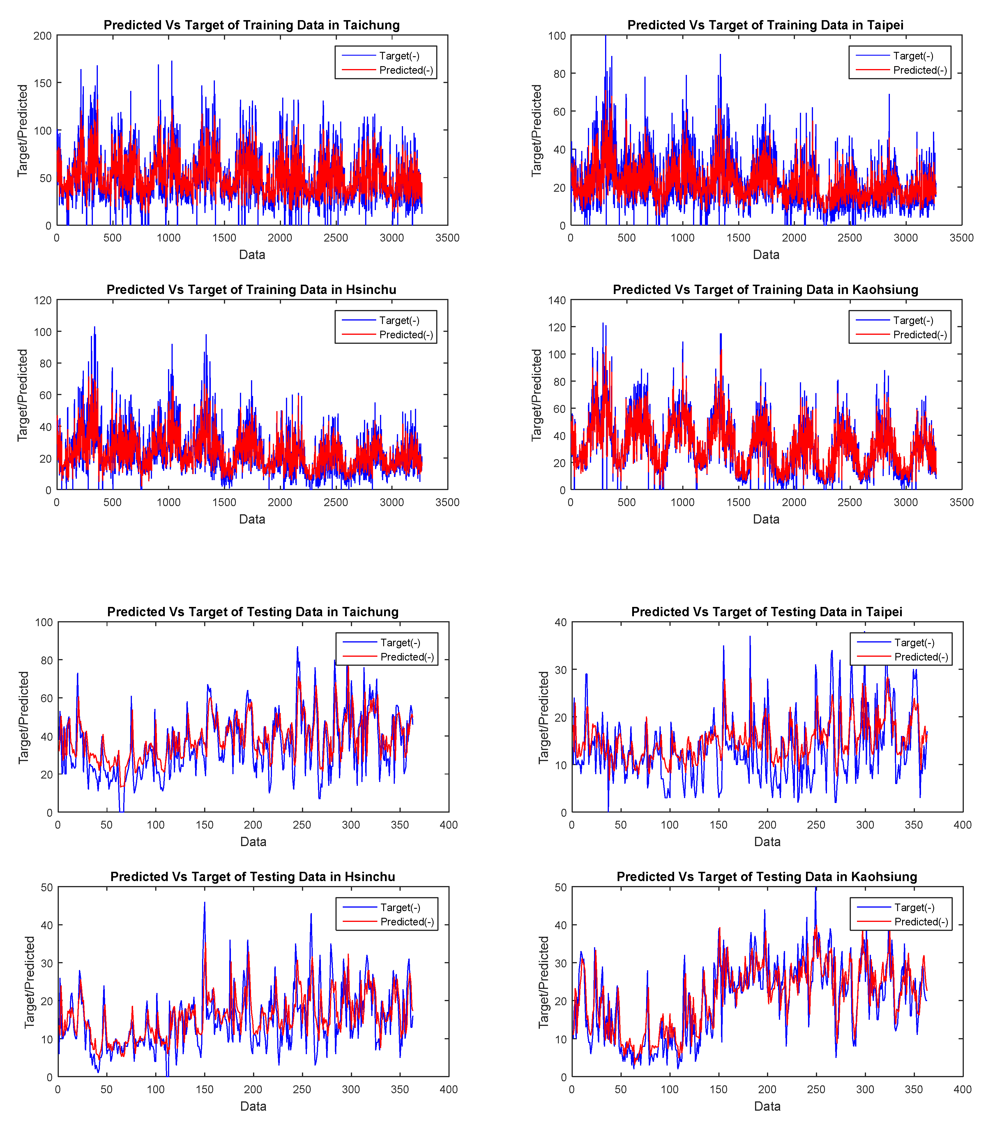
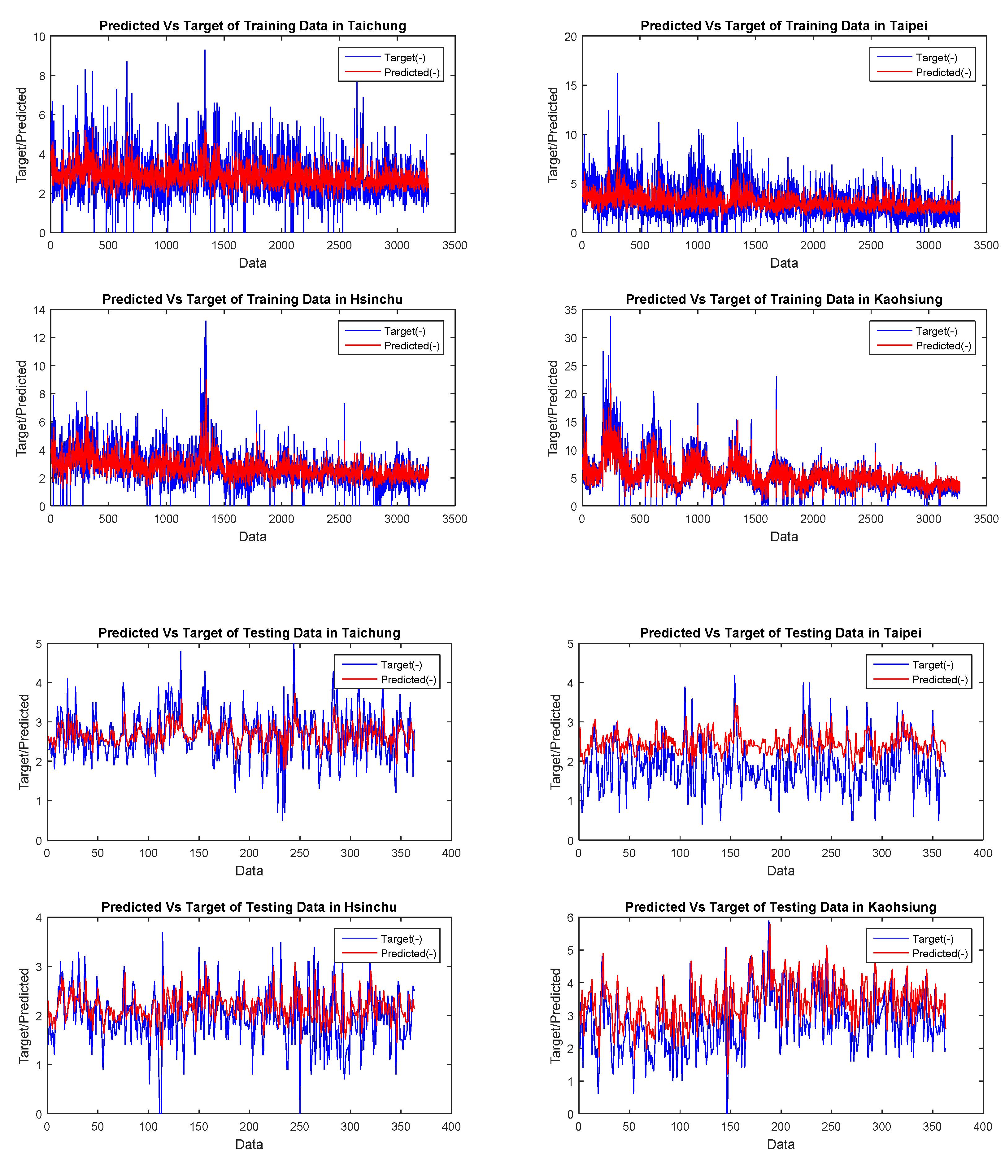
3.3. Air Pollution Forecasting Using VAR-Cascade-GA

Poor air quality in Taiwan has mostly been identified as being a result of household burning, largely the source of greenhouse gas emissions. Taiwan’s geography was observed to be a primary contributor towards its environmental problems, resulting in poor absorption and pollutant locking. Taipei, Taiwan’s capital and most populous city, is surrounded by mountains, and advanced manufacturing offices all along the western and northern coastlines of Taiwan were also built near mountain ranges. In Section 3, we already discussed the construction step and simulation studies. Furthermore, during the construction stage of input, we employed the VAR pollution space–time dataset including Taichung (Y₁), Taipei (Y₂), Hsinchu (Y₃), and Kaohsiung (Y₄) in Taiwan.

Figure 2 shows that five hidden layers were used to create the model, and the ratio used was calculated by assessing the error values of the testing results shown in

Table 2. Model comparison based on pollution.

Pollution	Portion	Training			Testing			Average			Elapsed Time
		RMSE	MAE	SMAPE	RMSE	MAE	SMAPE	RMSE	MAE	SMAPE
PM2.5	50:50	9.84	6.89	3.91	7.89	5.70	3.83	8.87	6.30	3.87	76.42
PM10		13.53	9.57	3.84	11.37	8.05	3.86	12.45	8.81	3.85	71.86
NOX		5.53	3.55	6.94	4.37	2.73	6.95	4.95	3.14	6.95	74.23
SO2		1.72	1.18	3.60	1.15	0.80	3.61	1.44	0.99	3.61	75.51
PM2.5	60:40	9.86	6.88	3.89	7.41	5.42	3.57	8.63	6.15	3.73	76.56
PM10		13.49	9.54	3.76	10.67	7.57	3.56	12.08	8.55	3.66	75.24
NOX		6.48	3.48	6.93	4.10	2.65	6.24	5.29	3.06	6.59	73.15
SO2		1.65	1.13	3.48	1.07	0.80	3.43	1.36	0.97	3.46	76.13
PM2.5	70:30	9.43	6.62	3.83	7.13	5.27	3.50	8.28	5.95	3.67	71.13
PM10		13.30	9.29	3.74	10.09	7.13	3.74	11.70	8.21	3.74	77.87
NOX		5.31	3.36	6.98	4.01	2.54	7.12	4.66	2.95	7.05	74.41
SO2		1.60	1.09	3.36	1.00	0.77	3.41	1.30	0.93	3.38	80.90
PM2.5	80:20	9.25	6.46	3.81	6.83	4.99	3.50	8.04	5.73	3.65	74.25
PM10		13.10	9.07	3.74	9.19	6.56	4.13	11.14	7.82	3.93	74.25
NOX		5.25	3.29	7.11	3.79	2.49	6.68	4.52	2.89	6.90	72.37
SO2		1.54	1.05	3.42	0.92	0.70	3.36	1.23	0.88	3.39	80.24
PM2.5	90:10 *	9.03	6.34	3.77	6.78	4.94	3.47	7.90	5.64	3.62	83.83
PM10		12.77	8.85	3.77	8.02	5.93	4.09	10.40	7.39	3.93	75.00
NOX		5.11	3.20	6.90	3.70	2.43	6.53	4.40	2.81	6.72	80.47
SO2		1.48	1.10	3.37	0.80	0.62	2.77	1.14	0.86	3.07	71.71

Noted: Best simulation with low error (*) and yellow highlight represent the lowest value of each information pollution, accuracy measurement, and elapsed time.

. During training and testing, PM_2.5 is represented in Figure 3, PM₁₀ is represented in Figure 4, NO_X is represented in Figure 5, and SO₂ is represented in Figure 6. In this context, the cascade neural network genetic algorithm model can be used to study nonlinear and nonstationary data on air pollution. The metrics used to evaluate the test set’s result were the root-mean-squared error (RMSE), mean absolute error (MAE), and symmetry mean absolute percentage (sMAPE) between the actual air pollution values and the predicted values. These are metrics that are commonly used in regression problems like our air pollution prediction. If all the metric values are smaller, then the model’s performance is better [25].

In the results, the cascade neural network genetic algorithm with ratio 90:10 provided lower RMSE, MAE, and sMAPE values for all variables. The optimum number of hidden neurons showing good performance in the test and validation results could then be selected. Using this model, a prediction of future air pollution was performed. In this study area, the air pollution levels in these four cities in Taiwan influence each other. However, the accuracy of prediction was not improved when we set the training and testing ratio to 80:20, 70:30, 60:40, or 50:50 in the same section. There are several training algorithms, such as backpropagation, Conjugate Gradient Powell–Beale (CGB), Broyden–Fletcher–Goldfarb (BFG), Levenberg–Marquardt (LM), and Scaled Conjugate Gradient (SCG). The rate of change in the error with respect to the connection weight including the error gradient is used as a path for training.

In order to measure the stage size to optimize performance, we used backpropagation and conducted a search along the conjugate or orthogonal path. Appropriately, we proved that this was the easiest way to train moderate feedback networks. That being said, some matrix multiplication is included in the processing for such issues as air pollution over time. The network is very wide in this research, so using backpropagation is a good way. When overfitting occurs, the transferability of the potential is significantly decreased. To suppress overfitting, methods such as so-called regularization are often used. L1 (L2) regularization adds the sum of the absolute (square) values of weights to the loss function, as in Equations (13) and (14), where $\mathsf{\Gamma }$ is the loss function and $w_{jk}^i$ indicates the weights in the network. In addition, $\mathsf{\alpha }$ is the scaling factor for the summation. $N_H$ denotes the number of layers and $N_i$ denotes the number of nodes in the $i$th layer.

$${\mathsf{\Gamma }}_{L1}=\mathsf{\Gamma }+\mathsf{\alpha } {\displaystyle \sum }_{i=1}^{N_H-1}{\displaystyle \sum }_{j=1}^{N_i}{\displaystyle \sum }_{k=1}^{N_{i+1}}\left|w_{jk}^i\right|$$

(13)

$${\mathsf{\Gamma }}_{L2}=\mathsf{\Gamma }+\mathsf{\alpha } {\displaystyle \sum }_{i=1}^{N_H-1}{\displaystyle \sum }_{j=1}^{N_i}{\displaystyle \sum }_{k=1}^{N_{i+1}}{(w_{jk}^i)}^2$$

(14)

3.4. Does the Activation Function Provide High Accuracy and Speed Up the Time Lapse?

Linear regression models work well throughout short-term predictions based on daily or weekly measurements in time series forecasting, but they cannot tackle nonlinearity in showing variables properly, not even for long-term predictions from seasonal or annual data series. Various machine learning methodologies have been introduced and used to simulate problems and provide predictions in environmental research, as machine efficiency has been evolving rapidly in the last decade. Despite its prominence and outstanding data accuracy, critical issues in the Artificial Neural Network are its propensity to overfit training data and inconsistency for short histories of training data. Several strategies for more effective and efficient preparation of NNs have been recommended. However, these are not simple and also have markedly poor accuracy.

After the training and testing comparisons already discussed in Section 3.3, we considered proving the performance of the hybrid cascade neural network genetic algorithm when using other activation functions. Computational capabilities are increasing in the era of big data, high-performance computing, parallel processing, and cloud computing. In line with this, we address whether the activation function can improve accuracy and speed up the time lapse. Throughout the last decades, the machine learning domain, a branch of artificial intelligence, has gained popularity, and researchers in the area have led it to expand through various areas of human life. Machine learning is a part of research that employs statistics and computer science concepts to develop mathematical models used to execute large tasks such as estimation and inference [55]. These frameworks are collections of mathematical interactions between the system’s inputs and outputs. A learning process entails predicting the model parameters so that the task can be executed effectively. To improve accuracy, researchers have conducted simulated comparisons using various activation functions. The most popular activation functions are SoftMax, tanh, ReLU, Leaky ReLU, sigmoid, and logsig [56,57,58,59].

As asserted, the activation function can be defined and applied to an ANN to assist the network in understanding various systems in data. Although contrasted to a neuron-based design seen in human brains, an activation function is essentially responsible for determining what neuron to trigger immediately [60]. Inside an ANN, the activation function is doing the same thing. All of this receives a prior nerve cell output signal and transforms it into a format which can be used as feedback to yet another cell. In this simulation, we used logsig in Equation (15), radbas in Equation (16), SoftMax in Equation (17), and tribas in Equation (18).

$$z_j=\frac{1}{1+\exp \left(-X_j\right)}$$

(15)

$$z\left(x\right)={\displaystyle \sum }_{i=1}^N{w}_i\phi (\Vert x-x_i\Vert )$$

(16)

$$\sigma {(\overrightarrow{z})}_i=\frac{e^{z_i} }{{\sum }_{j=1}^K{e}^{z_j}}$$

(17)

$$tri\left(x\right)=\mathsf{\Lambda }\left(x\right)\stackrel{\mathrm{def}}{=}\max \left(1-\left|x\right|,0\right)$$

(18)

Table 3. Combining activation functions with the Cascade Neural Network.

Pollution	Activation Function	Training			Testing			Average			Elapsed Time
		RMSE	MAE	SMAPE	RMSE	MAE	SMAPE	RMSE	MAE	SMAPE
PM2.5	logsig	9.02	6.30	3.77	6.77	4.94	3.54	7.90	5.62	3.66	78.03
PM10		12.79	8.86	3.71	8.12	6.02	4.05	10.46	7.44	3.88	75.48
NOX		5.04	3.15	6.84	3.79	2.43	6.62	4.42	2.79	6.73	72.43
SO2		1.48	1.01	3.35	0.82	0.63	3.00	1.15	0.82	3.18	76.59
PM2.5	radbas	9.06	6.37	3.80	6.80	5.00	3.51	7.93	5.69	3.66	80.97
PM10		12.79	8.85	3.79	8.11	6.03	4.19	10.45	7.44	3.99	74.77
NOX		5.09	3.16	6.83	3.75	2.40	6.19	4.42	2.78	6.51	82.35
SO2		1.49	1.01	3.36	0.83	0.64	2.93	1.16	0.83	3.15	73.33
PM2.5	SoftMax	9.07	6.35	3.78	6.70	4.91	3.46	7.89	5.63	3.62	75.47
PM10		12.81	8.90	3.75	8.13	6.04	4.24	10.47	7.47	3.99	74.70
NOX		5.11	3.19	7.12	3.64	2.35	6.23	4.38	2.77	6.67	72.11
SO2		1.48	1.01	3.42	0.84	0.66	3.12	1.16	0.84	3.27	77.53
PM2.5	tribas	9.03	6.34	3.80	6.81	4.97	3.52	7.92	5.66	3.66	93.20
PM10		12.81	8.90	3.75	8.13	6.04	4.24	10.47	7.47	3.99	74.70
NOX		5.13	3.21	6.98	3.68	2.37	6.53	4.41	2.79	6.75	72.29
SO2		1.49	1.01	3.36	0.84	0.65	2.94	1.16	0.83	3.15	80.35

Noted: Yellow highlight represent the lowest value of each information pollution, accuracy measurement, and elapsed time.

shows that the best activation function for PM₁₀ was logsig, that for PM_2.5 was SoftMax, that for NO_x was radbas, and that for SO₂ was tribas. The SoftMax activation function provided a shorter time lapse than other activation functions.

The cascade feed forward neural network model differs only when determining the input variables. During the simulation, we constructed the input by vector autoregression. Then, we considered the input as the lag variable of each predicted variable, in this case, the air pollution data at the four locations of Taichung, Taipei, Hsinchu, and Kaohsiung. Then, in the CFNN model for the four locations, neurons were compiled in the layer and the signal from the input to the first input layer, then to the second layer (hidden layer), and finally to the output layer. The general equation for forecasting pollution data in the four locations, represented in Equation (19), was used for prediction purposes in these study areas. Meanwhile, Equation (20) shows four input neurons $Y_{t-1}$ (lag 1) and five neurons in hidden layer of $Z_t$. To perform the forecasting, we used Equation (21) for NO_x with the radial basis activation function, Equation (22) for PM_2.5 with the SoftMax activation function, Equation (20) for PM₁₀ with the logsig activation function, and Equation (23) for SO₂ with the tribas activation function. We provide the results of forecasting in Figure 7 for the next 30 steps. The results show Taichung constantly leading with the highest pollutant score compared to other cities in Taiwan.

$$\begin{gathered} \widehat{{\mathit{Y}}_t}={\psi }_2\left\{\left[w_{b0} w_0 w_{i2}\right] \left[\begin{array}{c}1\\ Z_t\\ Y_{t-1}\end{array}\right]\right\} \\ {Z}_t={\psi }_2 \left(\left[\begin{array}{cc}{w}_{bi} & w_{i1} \end{array}\right] \left[\begin{array}{c}1\\ Y_{t-1}\end{array}\right]\right) \end{gathered}$$

(19)

Cascade Neural Network Genetic Algorithm for NO_x using the radial basis activation function:

$$\widehat{{\mathit{Y}}_t}=\left[\begin{array}{cccccccccc}-0.1244& -0.0992& 0.01054& -7.4544& 0.2238& -6.9588& 0.5603& 0.0444& -0.0689& 0.0770\\ -0.2483& 0.0359& -0.0665& -6.6298& 1.0709& -1.7180& 0.0655& 0.2562& 0.3422& 0.0572\\ -0.4328& 0.0253& -0.0226& 4.9796& 0.8715& 5.0640& 0.1253& 0.0189& 0.3570& 0.0742\\ -0.2772& 0.0015& 0.1201& -4.45319& -0.1428& 4.9089& 0.1066& 0.0465& -0.0148& 0.5544\end{array}\right]\left[\begin{array}{c}\begin{array}{c}\begin{array}{c}\begin{array}{c}1\\ Z_1\\ Z_2\end{array}\\ Z_3\\ Z_4\end{array}\\ Z_5\\ Y_{1,t-1}\end{array}\\ Y_{2,t-1}\\ \begin{array}{c}{Y}_{3,t-1}\\ Y_{4,t-1}\end{array}\end{array}\right],$$

$$Z_t=radbas \left[\begin{array}{ccccc}5.0776& 6.4191& 0.0893& 0.7930& -0.2450\\ 0.8287& 4.8674& -2.4160& -3.1740& -0.7644\\ -6.9722& -4.2852& 9.1216& -3.0205& 8.5264\\ -9.6954& -12.9182& 5.3748& 18.2621& -5.5156\\ 7.7948& 2.5076& 2.6535& -9.1934& -9.4768\end{array}\right]\left[\begin{array}{c}\begin{array}{c}\begin{array}{c}1\\ Y_{1,t-1}\end{array}\\ Y_{2,t-1}\end{array}\\ Y_{3,t-1}\\ Y_{4,t-1}\end{array}\right]$$

(20)

Cascade Neural Network Genetic Algorithm for PM_2.5 using the SoftMax activation function:

$$\left[\begin{array}{cccccccccc}0.9653& -1.0657& 3.2999& -2.4456& -0.7936& -1.1990& 0.7359& 0.0491& -0.0690& 0.1124\\ 1.2965& -1.5045& 2.3489& 2.0493& -1.9046& -1.6001& 0.0225& 0.2826& 0.3253& 0.0500\\ 6.0285& -6.1880& 0.3716& 2.3998& -6.8009& -6.3181& 0.1929& -0.0279& 0.4639& 0.1170\\ 0.9319& -0.9456& 10.3730& 3.4200& -1.1032& -0.9099& 0.0890& 0.0227& 0.0463& 0.7191\end{array}\right]\left[\begin{array}{c}\begin{array}{c}\begin{array}{c}\begin{array}{c}1\\ Z_1\\ Z_2\end{array}\\ Z_3\\ Z_4\end{array}\\ Z_5\\ Y_{1,t-1}\end{array}\\ Y_{2,t-1}\\ \begin{array}{c}{Y}_{3,t-1}\\ Y_{4,t-1}\end{array}\end{array}\right],$$

$$Z_t=softmax \left[\begin{array}{ccccc}6.2714& -7.3511& -7.8139& -1.9507& 4.3787\\ -5.6864& -7.7599& -8.3507& -2.9367& -2.3266\\ -6.4463& -6.6875& 5.0926& 1.5264& -1.1062\\ -5.0961& -3.3109& 5.3424& 6.5753& -3.4388 \\ 3.6740& -2.6485& -6.2284& -6.7208& 4.4362\end{array}\right]\left[\begin{array}{c}\begin{array}{c}\begin{array}{c}1\\ Y_{1,t-1}\end{array}\\ Y_{2,t-1}\end{array}\\ Y_{3,t-1}\\ Y_{4,t-1}\end{array}\right]$$

(21)

Cascade Neural Network Genetic Algorithm for PM₁₀ using the logsig activation function:

$$\widehat{{\mathit{Y}}_t}=\left[\begin{array}{cccccccccc}4.7332& -0.0171& -4.7892& -0.0294& -0.0499& -0.0380& 0.5673& 0.0698& 0.0402& 0.0720\\ -4.7021& 0.0480& 4.5307& -0.0609& 0.0313& -0.1244& 0.1252& 0.3677& 0.1878& 0.0614\\ 2.2770& 0.0263& -2.4010& -0.0006& -0.0102& 0.0014& 0.2351& -0.0648& 0.5960& 0.0696\\ 1.5241& -0.0534& -1.4885& 0.0533& -0.1240& 0.1097& 0.1118& 0.1017& 0.1786& 0.5507\end{array}\right]\left[\begin{array}{c}\begin{array}{c}\begin{array}{c}\begin{array}{c}1\\ Z_1\\ Z_2\end{array}\\ Z_3\\ Z_4\end{array}\\ Z_5\\ Y_{1,t-1}\end{array}\\ Y_{2,t-1}\\ \begin{array}{c}{Y}_{3,t-1}\\ Y_{4,t-1}\end{array}\end{array}\right],$$

$$Z_t=logsig \left[\begin{array}{ccccc}-7.6484& -5.6012& 5.5769& 0.2050& -7.1292\\ 9.0472& -2.0909& -7.4709& 4.9145& -5.3312\\ -4.1385& -9.9840& -3.4291& 6.0077& 2.4277\\ -1.5068& -4.0147& 3.5676& 5.6306& -9.0051 \\ -5.6488& 5.5027& 6.1290& 7.2003& 6.3822\end{array}\right]\left[\begin{array}{c}\begin{array}{c}\begin{array}{c}1\\ Y_{1,t-1}\end{array}\\ Y_{2,t-1}\end{array}\\ Y_{3,t-1}\\ Y_{4,t-1}\end{array}\right]$$

(22)

Cascade Neural Network Genetic Algorithm for SO₁₀ using the tribas activation function:

$$\widehat{{\mathit{Y}}_t}=\left[\begin{array}{cccccccccc}-0.1116& 5.1674& -0.0036& -0.0166& -3.4727& -0.2061& 0.4570& 0.0222& 0.0743& 0.0524\\ -0.2789& -1.0341& -0.0087& -0.0114& 7.8267& 0.1241& 0.0817& 0.3550& 0.1215& 0.0309\\ -0.8104& -7.8058& -0.0085& 0.0234& 5.2240& 0.0292& 0.1364& 0.0647& 0.4179& 0.1027\\ -0.1772& 6.5887& -0.0242& -0.0490& 6.7444& 0.0271& 0.0246& 0.0067& 0.0693& 0.6512\end{array}\right]\left[\begin{array}{c}\begin{array}{c}\begin{array}{c}\begin{array}{c}1\\ Z_1\\ Z_2\end{array}\\ Z_3\\ Z_4\end{array}\\ Z_5\\ Y_{1,t-1}\end{array}\\ Y_{2,t-1}\\ \begin{array}{c}{Y}_{3,t-1}\\ Y_{4,t-1}\end{array}\end{array}\right],$$

$$Z_t=tribas \left[\begin{array}{ccccc}7.3483& -2.1911& -8.1641& 0.4300& -3.6214\\ -1.5728& -2.5029& -10.1020& 0.5066& 7.0828\\ -5.3810& -9.9016& 7.7806& -2.1473& 5.0866\\ -1.1201& 10.2142& 6.6401& 6.7203& 4.0480\\ -2.9485& 8.1185& 7.2550& 8.2102& -8.3387\end{array}\right]\left[\begin{array}{c}\begin{array}{c}\begin{array}{c}1\\ Y_{1,t-1}\end{array}\\ Y_{2,t-1}\end{array}\\ Y_{3,t-1}\\ Y_{4,t-1}\end{array}\right]$$

(23)

4. Conclusions

In this paper, we first presented a full review of a cascade neural network with a genetic algorithm as applied to space–time forecasting. Experimental results on an air pollution dataset showed that our hybrid methods provide high accuracy as proved by the RMSE, MAE, and sMAPE values. Attributable to its rapid urbanization and industrialization over the last decades, Taiwan faces serious environmental issues, including air pollution. In order to resolve air quality issues, the government has taken several countermeasures. The attempt to eliminate SO₂ and overall suspended particulate matter was very effective when ever-increasing cars threatened city atmospheres with NOx and particulates. A space–time air pollution analysis over the last 10 years using the monitoring data clearly showed that with urban planning and countermeasure policies, air quality has improved. The analysis should be used to make future policy decisions. Air pollution temporal features were examined herein for Taiwan. The pattern from pollutants to particulates differs in air quality for each location. In a nutshell, the PM, SO₂, and NO_x levels have drastically increased. Future research should examine using VAR-SARIMA, VAR-ARCH, and other traditional time series as input.

References

1. Querol, X.; Alastuey, A.; Ruiz, C.R.; Artiñano, B.; Hansson, H.C.; Harrison, R.M.; Buringh, E.; Ten Brink, H.M.; Lutz, M.; Bruckmann, P.; et al. Speciation and origin of PM10 and PM2.5 in selected European cities. Atmos. Environ. 2004, 38, 6547–6555. [Google Scholar] [CrossRef]
2. Fan, J.; Wu, L.; Ma, X.; Zhou, H.; Zhang, F. Hybrid support vector machines with heuristic algorithms for prediction of daily diffuse solar radiation in air-polluted regions. Renew. Energy 2020, 145, 2034–2045. [Google Scholar] [CrossRef]
3. Masseran, N.; Safari, M.A.M. Intensity–duration–frequency approach for risk assessment of air pollution events. J. Environ. Manag. 2020, 264, 110429. [Google Scholar] [CrossRef] [PubMed]
4. Masseran, N.; Safari, M.A.M. Modeling the transition behaviors of PM 10 pollution index. Environ. Monit. Assess. 2020, 192, 441. [Google Scholar] [CrossRef] [PubMed]
5. De Vito, S.; Piga, M.; Martinotto, L.; Di Francia, G. CO, NO2 and NOx urban pollution monitoring with on-field calibrated electronic nose by automatic bayesian regularization. Sens. Actuators B Chem. 2009, 143, 182–191. [Google Scholar] [CrossRef]
6. Winarso, K.; Yasin, H. Modeling of air pollutants SO2 elements using geographically weighted regression (GWR), geographically temporal weighted regression (GTWR) and mixed geographically temporalweighted regression (MGTWR). ARPN J. Eng. Appl. Sci. 2016, 11, 8080–8084. [Google Scholar]
7. Zhang, J.J.; Wei, Y.; Fang, Z. Ozone pollution: A major health hazard worldwide. Front. Immunol. 2019, 10, 2518. [Google Scholar] [CrossRef] [Green Version]
8. Bernstein, J.A.; Alexis, N.; Barnes, C.; Bernstein, I.L.; Bernstein, J.A.; Nel, A.; Peden, D.; Diaz-Sanchez, D.; Tarlo, S.M.; Williams, P.B. Health effects of air pollution. J. Allergy Clin. Immunol. 2004, 114, 1116–1123. [Google Scholar] [CrossRef]
9. Xing, Y.F.; Xu, Y.H.; Shi, M.H.; Lian, Y.X. The impact of PM2.5 on the human respiratory system. J. Thorac. Dis. 2016, 8, E69–E74. [Google Scholar]
10. Rossati, A. Global warming and its health impact. Int. J. Occup. Environ. Med. 2017, 8, 7–20. [Google Scholar] [CrossRef] [Green Version]
11. Suhartono, S.; Subanar, S. Development of model building procedures in wavelet neural networks for forecasting non-stationary time series. Eur. J. Sci. Res. 2009, 34, 416–427. [Google Scholar]
12. Suhermi, N.; Suhartono; Prastyo, D.D.; Ali, B. Roll motion prediction using a hybrid deep learning and ARIMA model. Procedia Comput. Sci. 2018, 144, 251–258. [Google Scholar] [CrossRef]
13. McCulloch, W.S.; Pitts, W. A logical calculus of the ideas immanent in nervous activity. Bull. Math. Biophys. 1943, 5, 115–133. [Google Scholar] [CrossRef]
14. Chen, R.C.; Dewi, C.; Huang, S.W.; Caraka, R.E. Selecting critical features for data classification based on machine learning methods. J. Big Data 2020, 7, 52. [Google Scholar] [CrossRef]
15. Caraka, R.E.; Lee, Y.; Chen, R.C.; Toharudin, T. Using Hierarchical Likelihood towards Support Vector Machine: Theory and Its Application. IEEE Access 2020, 8, 194795–194807. [Google Scholar] [CrossRef]
16. Mueller, J.-A.; Lemke, F. Self-Organising Data Mining: An Intelligent Approach to Extract Knowledge from Data. 1999. Available online: https://www.knowledgeminer.eu/pdf/sodm.pdf (accessed on 6 May 2021).
17. De Gooijer, J.G.; Hyndman, R.J. 25 years of time series forecasting. Int. J. Forecast. 2006, 22, 443–473. [Google Scholar] [CrossRef] [Green Version]
18. Kaimian, H.; Li, Q.; Wu, C.; Qi, Y.; Mo, Y.; Chen, G.; Zhang, X.; Sachdeva, S. Evaluation of different machine learning approaches to forecasting PM2.5 mass concentrations. Aerosol Air Qual. Res. 2019, 19, 1400–1410. [Google Scholar] [CrossRef] [Green Version]
19. Guo, Y.; Liu, Y.; Oerlemans, A.; Lao, S.; Wu, S.; Lew, M.S. Deep learning for visual understanding: A review. Neurocomputing 2016, 187, 27–48. [Google Scholar] [CrossRef]
20. Szandała, T. Review and comparison of commonly used activation functions for deep neural networks. arXiv 2020. Available online: https://arxiv.org/abs/2010.09458 (accessed on 6 May 2021).
21. Sony, S.; Dunphy, K.; Sadhu, A.; Capretz, M. A systematic review of convolutional neural network-based structural condition assessment techniques. Eng. Struct. 2021, 226, 111347. [Google Scholar] [CrossRef]
22. Caraka, R.E.; Chen, R.C.; Yasin, H.; Pardamean, B.; Toharudin, T.; Wu, S.H. Prediction of Status Particulate Matter 2.5 using State Markov Chain Stochastic Process and HYBRID VAR-NN-PSO. IEEE Access 2019, 7, 161654–161665. [Google Scholar] [CrossRef]
23. Kuster, C.; Rezgui, Y.; Mourshed, M. Electrical load forecasting models: A critical systematic review. Sustain. Cities Soc. 2017, 35, 257–270. [Google Scholar] [CrossRef]
24. Cios, K.J.; Pedrycz, W.; Swiniarski, R.W.; Kurgan, L.A. Data Mining: A Knowledge Discovery Approach; Springer: Boston, MA, USA, 2007; ISBN 9780387333335. [Google Scholar]
25. Makridakis, S.; Spiliotis, E.; Assimakopoulos, V. The M4 Competition: 100,000 time series and 61 forecasting methods. Int. J. Forecast. 2020, 36, 54–74. [Google Scholar] [CrossRef]
26. Makridakis, S.G.; Wheelwright, S.C.; Hyndman, R.J. Forecasting: Methods and Applications. J. Forecast. 1998, 1–656. [Google Scholar] [CrossRef]
27. Wong, K.W.; Wong, P.M.; Gedeon, T.D.; Fung, C.C. Rainfall prediction model using soft computing technique. Soft Comput. 2003, 7, 434–438. [Google Scholar] [CrossRef]
28. Hochreiter, S.; Schmidhuber, J. Long Short-Term Memory. Neural Comput. 1997, 9, 1735–1780. [Google Scholar] [CrossRef] [PubMed]
29. Mislan, M.; Haviluddin, H.; Hardwinarto, S.; Sumaryono, S.; Aipassa, M. Rainfall Monthly Prediction Based on Artificial Neural Network: A Case Study in Tenggarong Station, East Kalimantan—Indonesia. Procedia Comput. Sci. 2015, 59, 142–151. [Google Scholar] [CrossRef] [Green Version]
30. Darwin, C. The Correspondence of Charles Darwin: 1821–1860; Cambridge University Press: Cambridge, UK, 2002. [Google Scholar]
31. Pfeiffer, J.R. Evolutionary theory. In George Bernard Shaw in Context; Cambridge University Press: Cambridge, UK, 2015; ISBN 9781107239081. [Google Scholar]
32. Wuketits, F.M. Charles darwin and modern moral philosophy. Ludus Vitalis 2009, 17, 395–404. [Google Scholar]
33. García-Martínez, C.; Rodriguez, F.J.; Lozano, M. Genetic algorithms. In Handbook of Heuristics; Springer: Cham, Switzerland, 2018; ISBN 9783319071244. Available online: https://www.springer.com/gp/book/9783319071237 (accessed on 6 May 2021).
34. Sivanandam, S.; Deepa, S. Introduction to Genetic Algorithms; Springer: Berlin/Heidelberg, Germany, 2008. [Google Scholar]
35. Gupta, J.N.D.; Sexton, R.S. Comparing backpropagation with a genetic algorithm for neural network training. Omega 1999, 27, 679–684. [Google Scholar] [CrossRef]
36. Caraka, R.E.; Chen, R.C.; Yasin, H.; Lee, Y.; Pardamean, B. Hybrid Vector Autoregression Feedforward Neural Network with Genetic Algorithm Model for Forecasting Space-Time Pollution Data. Indones. J. Sci. Technol. 2021, 6, 243–266. [Google Scholar]
37. Kubat, M.; Kubat, M. The Genetic Algorithm. In An Introduction to Machine Learning; Springer International Publishing: Cham, Switzerland, 2017. [Google Scholar]
38. Moscato, P.; Cotta, C. A Modern Introduction to Memetic Algorithms. In Handbook of Metaheuristics; Springer: Boston, MA, USA, 2010; pp. 141–183. Available online: https://link.springer.com/chapter/10.1007/978-1-4419-1665-5_6 (accessed on 6 May 2021).
39. Makridakis, S.; Wheelwright, S.C. Forecasting Methods for Management. Oper. Res. Q. 1974, 25, 648–649. [Google Scholar] [CrossRef]
40. Makridakis, S. A Survey of Time Series. Int. Stat. Rev. Rev. Int. Stat. 1976, 44, 29. [Google Scholar] [CrossRef]
41. Warsito, B.; Santoso, R.; Suparti; Yasin, H. Cascade Forward Neural Network for Time Series Prediction. J. Phys. Conf. Ser. 2018, 1025, 012097. [Google Scholar] [CrossRef]
42. Schetinin, V. A learning algorithm for evolving cascade neural networks. Neural Process. Lett. 2003, 17, 21–31. [Google Scholar] [CrossRef]
43. Ding, S.; Zhao, H.; Zhang, Y.; Xu, X.; Nie, R. Extreme learning machine: Algorithm, theory and applications. Artif. Intell. Rev. 2015, 44, 103–115. [Google Scholar] [CrossRef]
44. Suhartono; Prastyo, D.D.; Kuswanto, H.; Lee, M.H. Comparison between VAR, GSTAR, FFNN-VAR and FFNN-GSTAR Models for Forecasting Oil Production Methods. Mat. Malays. J. Ind. Appl. Math. 2018, 34, 103–111. [Google Scholar]
45. Prastyo, D.D.; Nabila, F.S.; Lee, M.H.S.; Suhermi, N.; Fam, S.F. VAR and GSTAR-based feature selection in support vector regression for multivariate spatio-temporal forecasting. In Communications in Computer and Information Science; Springer: Singapore, 2018; pp. 46–57. [Google Scholar]
46. Zhang, P.G. Time series forecasting using a hybrid ARIMA and neural network model. Neurocomputing 2003, 50, 159–175. [Google Scholar] [CrossRef]
47. Geurts, M.; Box, G.E.P.; Jenkins, G.M. Time Series Analysis: Forecasting and Control. J. Mark. Res. 2006. [Google Scholar] [CrossRef]
48. McLeod, A.I.; Yu, H.; Mahdi, E. Time Series Analysis with R. Handb. Stat. 2011, 30, 661–672. [Google Scholar] [CrossRef]
49. Liao, W.T. Clustering of time series data—A survey. Pattern Recognit. 2005, 38, 1857–1874. [Google Scholar] [CrossRef]
50. Subba Rao, T. Time Series Analysis. J. Time Ser. Anal. 2010, 31, 139. [Google Scholar] [CrossRef]
51. Mudelsee, M. Climate Time Series Analysis: Regression; Springer: Dordrecht, The Netherlands, 2010; Volume 42, ISBN 978-90-481-9481-0. [Google Scholar]
52. Zhu, X.; Pan, R.; Li, G.; Liu, Y.; Wang, H. Network vector autoregression. Ann. Stat. 2017, 45, 1096–1123. [Google Scholar] [CrossRef] [Green Version]
53. Nourani, V.; Baghanam, A.H.; Adamowski, J.; Gebremichael, M. Using self-organizing maps and wavelet transforms for space-time pre-processing of satellite precipitation and runoff data in neural network based rainfall-runoff modeling. J. Hydrol. 2013, 476, 228–243. [Google Scholar] [CrossRef]
54. Ippoliti, L.; Valentini, P.; Gamerman, D. Space-time modelling of coupled spatiotemporal environmental variables. J. R. Stat. Soc. Ser. C Appl. Stat. 2012. [Google Scholar] [CrossRef]
55. Sharma, S.; Sharma, S. Understanding Activation Functions in Neural Networks. Int. J. Eng. Appl. Sci. Technol. 2017, 4, 310–316. [Google Scholar]
56. Apicella, A.; Donnarumma, F.; Isgrò, F.; Prevete, R. A survey on modern trainable activation functions. Neural Netw. 2021, 138, 14–32. [Google Scholar] [CrossRef]
57. Al-Rikabi, H.M.H.; Al-Ja’afari, M.A.M.; Ali, A.H.; Abdulwahed, S.H. Generic model implementation of deep neural network activation functions using GWO-optimized SCPWL model on FPGA. Microprocess. Microsyst. 2020, 77, 103141. [Google Scholar] [CrossRef]
58. Boob, D.; Dey, S.S.; Lan, G. Complexity of training ReLU neural network. Discret. Optim. 2020, 100620. [Google Scholar] [CrossRef]
59. Liu, B. Understanding the loss landscape of one-hidden-layer ReLU networks. Knowl. Based Syst. 2021, 220, 106923. [Google Scholar] [CrossRef]
60. Bouwmans, T.; Javed, S.; Sultana, M.; Jung, S.K. Deep neural network concepts for background subtraction: A systematic review and comparative evaluation. Neural Netw. 2019, 117, 8–66. [Google Scholar] [CrossRef] [Green Version]
Figure 1. An overview of the genetic algorithm training and evaluation phases.
Symmetry 13 01158 g001
Figure 2. Space–time Cascade Neural Network with genetic algorithm, adopted by [22,36].
Symmetry 13 01158 g002
Figure 3. PM2.5 data training of the CFNN using a genetic algorithm and backpropagation.
Symmetry 13 01158 g003
Figure 4. PM10 data training of the CFNN using a genetic algorithm and backpropagation.
Symmetry 13 01158 g004
Figure 5. NOx data training of the CFNN using a genetic algorithm and backpropagation.
Symmetry 13 01158 g005
Figure 6. SO2 data training of the CFNN using a genetic algorithm and backpropagation.
Symmetry 13 01158 g006
Figure 7. Forecasting all pollution datasets using the CFNN with a genetic algorithm and backpropagation.
Symmetry 13 01158 g007