Novel Approach for Third-Party Reverse Logistic Provider Selection Process under Linear Diophantine Fuzzy Prioritized Aggregation Operators

Abstract

Aggregation operators are fundamental concept for information fusion in real-life problems. Many researchers developed aggregation operators for multi-criteria decision-making (MCDM) under uncertainty. Unfortunately, the existing operators can be utilized under strict limitations and constraints. In this manuscript, we focused on new prioritized aggregation operators which remove the strict limitations of the existing operators. The addition of reference parameters associated with membership and non-membership grades in the linear Diophantine Fuzzy sets provide a robust modeling for MCDM problems. The primary objective of this manuscript is to introduce new aggregation operators for modeling uncertainty by using linear Diophantine Fuzzy information. For this objective we develop aggregation operators (AO) namely, "linear Diophantine Fuzzy prioritized weighted average" (LDFPWA) operator and "linear Diophantine Fuzzy prioritized weighted geometric" (LDFPWG) operator. Certain essential properties of new prioritized AOs are also proposed. A secondary objective is to discuss a practical application of third party reverse logistic provider (3PRLP) optimization problem. The efficiency, superiority, and rationality of the proposed approach is analyzed by a numerical example to discuss 3PRLP. The symmetry of optimal decision and ranking of feasible alternatives is followed by a comparative analysis.

1. Introduction

The problem of vague and misleading information has become a major issue for decades. Aggregation of data is important for decision-making in corporate, administrative, social, medical, technological, psychological, and artificial intelligence fields. Awareness of the alternative has traditionally been seen as a crisp number or linguistic number. However, due to its uncertainty, the data cannot easily be aggregated. MCDM is a commonly used cognitive activity tool, the main aim of which is to decide between a finite number of alternatives using the preference information provided by decision makers (DM). The MCDM method, however, tends to be ambiguous and inaccurate, because it involves the complexity of human reasoning abilities, finding it challenging for DMs in the review process which provide accurate evaluation. It is really essential to resolve this problem, in addition to dealing with unpredictability, Zadeh [1] has pioneered the sort of Fuzzy set (FS) theory. Atanassov [2,3] initiated the novel idea of intuitionistic Fuzzy set (IFS) Yager [4,5,6] introduced Pythagorean Fuzzy set (PFS) as an extension of IFS. IFS and PFS were newly generalized by Yager and the q-ROFS concept was developed. The limitation of q-ROFS would be that the total of the member-ship degree (MD) power and the non-membership degree (NMD) power of q may be less than or identical to one. Clearly, the greater the rung q, the more the bounding condition is fulfilled by orthopairs and, thus, the greater the space of Fuzzy data that can be expressed by q-ROFSs [7]. In ability to cope with both the complete absence of clarity and flouted information q-ROFs are more efficient than PFS and IFS.

Alcantud and Garcia [8] introduced a new criterion for soft set based decision making problems under incomplete information. Xu et al. [9,10] introduced many averaging and geometric operators related to IFS. Hashmi et al. [11] investigated clustering analysis and medical diagnosis based on m-polar neutrosophic set and m-polar neutrosophic topology. Wang and Liu [12], Zhang et al. [13], Zhao [14] et al., and Garg [15] introduced many decision making approaches for numerous extensions of Fuzzy sets. Mahmood et al. [16] proposed spherical Fuzzy decision-making approach with diagnosis application. Feng et al. [17] introduced Lexicographic orders for IFNs. Recently, Akram et al. [18,19] introduced Extensions of Dombi aggregation operators and Einstein geometric operators. Peng and Yang [20] presented novel features and properties of IFSs and their significant results. A robust MCDM approach based on PFS-TOPSIS is suggested by Zhang and Xu [21]. Karaaslan and Ozlu [22] introduced some correlation coefficients of dual type-2 hesitant Fuzzy sets. Sitara et al. [23] developed q-rung picture Fuzzy graph structures and new decision-making analysis based on graph structures.

Riaz and Hashmi [24] introduced the concept of linear Diophantine Fuzzy set (LDFS) as a generalized concept of IFS, PFS, and q-ROFS. Due to presence of reference parameters, LDFS is a new approach towards soft computing, uncertain decision-making analysis, optimization, and real-world problems. LDFSs have been extended to algebraic structures and LDF-coding theory [25], LDF-relations with decision making [26], q-LDFS with emergency decision support system for COVID19 [27]. Pamucar [28] introduced normalized weighted geometric Dombi Bonferoni mean operator with interval grey numbers. Pamucar and Jankovic [29] established hybrid interval rough weighted power-Heronian operator for MCDM. Riaz et al. introduced the certain extensions of AOs like q-ROFS Einstein [30], prioritized [31], Einstein prioritized and some hybrid AOs [32,33]. Riaz et al. [34] introduced novel concept of bipolar picture Fuzzy.

IFSs, PFSs, and q-ROFs each have their own restrictions in terms of the sum of membership and non-membership degrees. Because of the varied conditions on the membership and non-membership degrees of IFSs, PFSs, and q-ROFs, decision makers are unable to freely evaluate diverse alternatives. To overcome this study gap, the LDFS theory has been suggested, in which decision maker can select grades freely ranging from 0 to 1 because of reference parameters. If we have a linear prioritized relationship among the criterion in LDF data. We do not have a tool for dealing with this type of issue; to deal with this form of MCDM, we will propose several types of prioritized AOs to aggregate LDF data.

Several prioritized AOs were introduced by Yager [35]. According to Yager, in such situations, we should not permit the budget advantage to reduce the effectiveness of protection, where we select a child’s bike based on safety and cost criteria. Then there’s a sort of priority relationship between these two criterion, with protection taking precedence. This situation is known as an aggregation problem since the attributes have a priority relationship. The AOs in question, such as the average operator and the geometric operator, are significant because we want to consider higher priority criteria, such as safety in the case of the former, are no longer viable. In this case, Yager [35] provided prioritized AOs by modeling attribute prioritization in terms of criterion weights based on fulfillment of the higher importance attributes. New aggregation operators and decision-making method are developed by numerous researchers [36,37,38,39,40].

To choose a suitable 3PRLP as a business partner, a manufacturer must first evaluate the 3PRLPs. The business (i.e., the shipper) would weigh the relative weights of the 3PRLPs and assign the transporting volumes to the 3PRLP with the highest weight. In general, 3PRLP assessment is a multi-criteria task that necessitates the consideration of several physical and intellectual criteria. To put it another way, choosing the right 3PRLP requires much more than just comparing prices. Despite the fact that there has recently been a considerable amount of study on 3PRLP evaluations, and numerous evaluation criteria have been developed. The most widely used parameters, according to Aguezzoul’s Pareto analysis, are cost, relationship, facilities, efficiency, equipment, framework, adaptability, and timeliness [41]. Prahinski and Kocabasoglu [42] suggest many justifications for the intense demand in RLs around the world. Overall, RLs offers companies a tactical strategic advantage over competitors who do not use it, while also increasing client retention rates. This type of logistics assures consumers that they can quickly return defective or damaged goods and that the recycled parts of their goods can be reused. Furthermore, environmental activists’ and governments’ concerns have compelled business leaders to prioritize efficient remanufacturing, recycling, and preservation in all areas of RLs [43].

First, we highlight the main objectives of this manuscript as follows: (1) To introduce new aggregation operators for modeling uncertainty by using linear Diophantine Fuzzy information. For this objective, we develop new aggregation operators named as LDFPWA and LDFPWG. These operators remove the strict limitations of the existing operators; (2) To discuss certain essential properties of new prioritized aggregation operators; (3) To use the idea of score function for ranking of feasible alternatives; (4) To present a practical application of third party reverse logistic provider (3PRLP) optimization problem; (5) The efficiency, superiority, and rationality of the proposed approach is analyzed by a numerical example. A comparative analysis is presented to discuss the symmetry of optimal decision and ranking of feasible alternatives.

The rest of the paper is arranged as follows. Section 2 includes research background and literature related to 3PRLP selection and criterion regarding to 3PRLP. Section 3 consists of basic concepts of LDFS. Section 4 develops a variety of LDF prioritized AOs. Section 5 presents an MCGDM framework to the suggested AOs, as well as numerical example. Section 6 summaries the study paper’s key findings.

2. Preliminaries

In this section, we will review some LDFS’s fundamentals.

Definition 1

([24]). A LDFS ℜ in universe Λ is defined as

$$\Re =\left\{\left(\varsigma ,\langle {\mathcal{Y}}_{\Re }(\varsigma ),{\mathcal{X}}_{\Re }(\varsigma )\rangle ,\langle {\mathcal{D}}_{\Re }(\varsigma ),{\mathcal{Z}}_{\Re }(\varsigma )\rangle \right):\varsigma \in \Lambda \right\},$$

where ${\mathcal{Y}}_{\Re }(\varsigma ),{\mathcal{X}}_{\Re }(\varsigma ),{\mathcal{D}}_{\Re }(\varsigma ),{\mathcal{Z}}_{\Re }(\varsigma )\in [0,1]$ are the MD, the NMD, and the corresponding reference parameters, respectively. Moreover,

$$0\le {\mathcal{D}}_{\Re }(\varsigma )+{\mathcal{Z}}_{\Re }(\varsigma )\le 1,$$

and

$$0\le {\mathcal{D}}_{\Re }(\varsigma ){\mathcal{Y}}_{\Re }(\varsigma )+{\mathcal{Z}}_{\Re }(\varsigma ){\mathcal{X}}_{\Re }(\varsigma )\le 1$$

for all $\varsigma \in \Lambda$. The LDFS

$${\Re }_{\Lambda }=\{(\varsigma ,\langle 1,0\rangle ,\langle 1,0\rangle ):\varsigma \in \Lambda \}$$

is known the absolute LDFS in Λ. The LDFS

$${\Re }_{\varphi }=\{(\varsigma ,\langle 0,1\rangle ,\langle 0,1\rangle ):\varsigma \in \Lambda \}$$

is known the null LDFS in Λ.

The reference parameters may be used to model or classify specific structures. By modifying the physical meaning of the reference parameters, we can classify various systems. In addition,

${\eta }_{\Re }(\varsigma ){\pi }_{\Re }(\varsigma )=1-({\mathcal{D}}_{\Re }(\varsigma ){\mathcal{Y}}_{\Re }(\varsigma )+{\mathcal{Z}}_{\Re }(\varsigma ){\mathcal{X}}_{\Re }(\varsigma ))$ is called the indeterminacy degree and its corresponding reference parameter of $\varsigma$ to ℜ.

In this framework, the set of reference parameters is very significant. They help us to increased the valuation space of MD and NMD functions and parameterize the model, which gives us variety of taking alternative under different physical situations. The deficiency in IFS, PFS, and q-ROFS is that they have no parameterizations. This novel idea enhances the existing methodologies and we can freely choose the grades without any limitation.

Many researchers [7] worked on the novel idea of q-ROFSs which is the generalization of IFS and PFS with the condition $0\le {\mathcal{Y}}_{\mathcal{O}}^q(\varsigma )+{\mathcal{X}}_{\mathcal{O}}^q(\varsigma )\le 1$. When “q” is very large then graphically this set is coincide with LDFS but the deficiency is that in q-ROFS we have no parameterizations, which is an additional factor in LDFSs. For small values of “q”, the valuation space of q-ROFS is less than that of LDFSs and cannot handle uncertainties completely in decision making problems. For the input data in MADM problems if we have ${\mathcal{Y}}_{\mathcal{O}}^q(\varsigma )$ and ${\mathcal{X}}_{\mathcal{O}}^q(\varsigma )$ equal to 1, then we cannot deal these inputs with q-ROFS (i.e., $1+1>1$), but with the suitable choice of reference parameters we can easily deal these types of values in LDFSs (i.e., $\left(1\right)\left(0.6\right)+\left(1\right)\left(0.3\right)<1$; the choice of numeric values of reference parameters is according to the situation and decision-making problem with the condition that there sum is less than 1). From all the discussion it is clear that our proposed idea is more suitable and superior to others and contains a variety of reference parameters. We can use this approach in various applications of engineering, medical, artificial intelligence, and MADM methods. In

Table 1. Comparison between LDFS with some existing concepts.

Concepts	Remarks
Fuzzy sets [1]	It does not consider NMD.
IFSs [2]	It cannot be applied if $1<{\mathcal{Y}}_{\mathcal{I}}(\varsigma )+{\mathcal{X}}_{\mathcal{I}}(\varsigma )\le 2$ for some $\varsigma$.
PFSs [5,6]	It cannot be applied if $1<{\mathcal{Y}}_{\mathcal{P}}^2(\varsigma )+{\mathcal{X}}_{\mathcal{P}}^2(\varsigma )\le 2$ for some $\varsigma$.
q-ROFSs [7]	It is inapplicable for smaller “q” values. with $1<{\mathcal{Y}}_{\mathcal{O}}^q(\varsigma )+{\mathcal{X}}_{\mathcal{O}}^q(\varsigma )\le 2$, or if ${\mathcal{Y}}_{\mathcal{O}}(\varsigma )={\mathcal{X}}_{\mathcal{O}}(\varsigma )=1$ for some $\varsigma$.
LDFSs [24]	(1) It can handle all situations where IFS, PFS, and q-ROFS cannot be used; (2) it takes a parameterizations approach and operates under the control of reference parameters; (3) MD and NMD can be taken in free manner from $[0,1]$.

, we can see the comparison between proposed approach with the existing concepts.

Definition 2

([24]). A linear Diophantine Fuzzy number (LDFN) is a tuple $\breve{\Omega }=(\langle {\mathcal{Y}}_{\breve{\Omega }},{\mathcal{X}}_{\breve{\Omega }}\rangle ,$$\langle {\mathcal{D}}_{\breve{\Omega }},{\mathcal{Z}}_{\breve{\Omega }}\rangle )$ satisfying the following conditions:

(1)

$0\le {\mathcal{Y}}_{\breve{\Omega }},{\mathcal{X}}_{\breve{\Omega }},{\mathcal{D}}_{\breve{\Omega }},{\mathcal{Z}}_{\breve{\Omega }}\le 1$;

(2)

$0\le {\mathcal{D}}_{\breve{\Omega }}+{\mathcal{Z}}_{\breve{\Omega }}\le 1$;

(3)

$0\le {\mathcal{D}}_{\breve{\Omega }}{\mathcal{Y}}_{\breve{\Omega }}+{\mathcal{Z}}_{\breve{\Omega }}{\mathcal{X}}_{\breve{\Omega }}\le 1$.

Definition 3

([24]). Let $\breve{\Omega }=(\langle {\mathcal{Y}}_{\breve{\Omega }},{\mathcal{X}}_{\breve{\Omega }}\rangle ,\langle {\mathcal{D}}_{\breve{\Omega }},{\mathcal{Z}}_{\breve{\Omega }}\rangle )$ be a LDFN, then score function $(✠\breve{\Omega })$ can be define by the mapping $✠\left(\breve{\Omega }\right):LDFN(\Lambda )\to [-1,1]$ and given by

$$✠\left(\breve{\Omega }\right)=\frac{1}{2}[({\mathcal{Y}}_{\breve{\Omega }}-{\mathcal{X}}_{\breve{\Omega }})+({\mathcal{D}}_{\breve{\Omega }}-{\mathcal{Z}}_{\breve{\Omega }})]$$

where $LDFN(\Lambda )$ is an assemblage of LDFNs on Λ.

Definition 4

([24]). Let $\breve{\Omega }=(\langle {\mathcal{Y}}_{\breve{\Omega }},{\mathcal{X}}_{\breve{\Omega }}\rangle ,\langle {\mathcal{D}}_{\breve{\Omega }},{\mathcal{Z}}_{\breve{\Omega }}\rangle )$ be a LDFN, then accuracy function can be defined by the mapping $\psi :LDFN(\Lambda )\to [0,1]$ and given as

$$\psi \left(\breve{\Omega }\right)=\frac{1}{2}\left[\left(\frac{{\mathcal{Y}}_{\breve{\Omega }}+{\mathcal{X}}_{\breve{\Omega }}}{2}\right)+({\mathcal{D}}_{\breve{\Omega }}+{\mathcal{Z}}_{\breve{\Omega }})\right]$$

Definition 5

([24]). Let ${\breve{\Omega }}_1$ and ${\breve{\Omega }}_2$ be two LDFNs then by using the score function and accuracy function, we have:

(i) :

If $✠\left({\breve{\Omega }}_1\right)<✠\left({\breve{\Omega }}_2\right)$ then ${\breve{\Omega }}_1<{\breve{\Omega }}_2$,

(ii) :

If $✠\left({\breve{\Omega }}_2\right)<✠\left({\breve{\Omega }}_1\right)$ then ${\breve{\Omega }}_2<{\breve{\Omega }}_1$,

(iii) :

If $✠\left({\breve{\Omega }}_2\right)=✠\left({\breve{\Omega }}_1\right)$ then,

(a) :

If $\psi \left({\breve{\Omega }}_1\right)<\psi \left({\breve{\Omega }}_2\right)$ then ${\breve{\Omega }}_1<{\breve{\Omega }}_2$,

(b) :

If $\psi \left({\breve{\Omega }}_2\right)<\psi \left({\breve{\Omega }}_1\right)$ then ${\breve{\Omega }}_2<{\breve{\Omega }}_1$,

(c) :

If $\psi \left({\breve{\Omega }}_1\right)=\psi \left({\breve{\Omega }}_2\right)$ then ${\breve{\Omega }}_1={\breve{\Omega }}_2$.

Definition 6

([24]). Let $\breve{\Omega }=(\langle {\mathcal{Y}}_{\breve{\Omega }},{\mathcal{X}}_{\breve{\Omega }}\rangle ,\langle {\mathcal{D}}_{\breve{\Omega }},{\mathcal{Z}}_{\breve{\Omega }}\rangle )$ be a LDFN, another definition of score function is defined as expectation score function (ESF) on $LDFN(\Lambda )$ having range $\mathcal{H}:LDFN(\Lambda )\to [0,1]$ and define as

$$\mathcal{H}\left(\breve{\Omega }\right)=\frac{1}{2}\left[\frac{({\mathcal{Y}}_{\breve{\Omega }}-{\mathcal{X}}_{\breve{\Omega }}+1)}{2}+\frac{({\mathcal{D}}_{\breve{\Omega }}-{\mathcal{Z}}_{\breve{\Omega }}+1)}{2}\right]$$

Definition 7

([24]). Let ${\breve{\Omega }}_i=(\langle {\mathcal{Y}}_i,{\mathcal{X}}_i\rangle ,\langle {\mathcal{D}}_i,{\mathcal{Z}}_i\rangle )$ be two LDFNs with $i=1,2$. Then

• ${\breve{\Omega }}_1\subseteq {\breve{\Omega }}_2\iff {\mathcal{Y}}_1\le {\mathcal{Y}}_2,{\mathcal{X}}_2\le {\mathcal{X}}_1,{\mathcal{D}}_1\le {\mathcal{D}}_2,{\mathcal{Z}}_2\le {\mathcal{Z}}_1$;
• ${\breve{\Omega }}_1={\breve{\Omega }}_2\iff {\mathcal{Y}}_1={\mathcal{Y}}_2,{\mathcal{X}}_1={\mathcal{X}}_2,{\mathcal{D}}_1={\mathcal{D}}_2,{\mathcal{Z}}_1={\mathcal{Z}}_2$;
• ${\breve{\Omega }}_1\oplus {\breve{\Omega }}_2=\left(\langle {\mathcal{Y}}_1+{\mathcal{Y}}_2-{\mathcal{Y}}_1{\mathcal{Y}}_2,{\mathcal{X}}_1{\mathcal{X}}_2\rangle ,\langle {\mathcal{D}}_1+{\mathcal{D}}_2-{\mathcal{D}}_1{\mathcal{D}}_2,{\mathcal{Z}}_1{\mathcal{Z}}_2\rangle \right)$;
• ${\breve{\Omega }}_1\otimes {\breve{\Omega }}_2=\left(\langle {\mathcal{Y}}_1{\mathcal{Y}}_2,{\mathcal{X}}_1+{\mathcal{X}}_2-{\mathcal{X}}_1{\mathcal{X}}_2\rangle ,\langle {\mathcal{D}}_1{\mathcal{D}}_2,{\mathcal{Z}}_1+{\mathcal{Z}}_2-{\mathcal{Z}}_1{\mathcal{Z}}_2\rangle \right)$.
• ${\breve{\Omega }}_1^c=(\langle {\mathcal{X}}_1,{\mathcal{Y}}_1\rangle ,\langle {\mathcal{Z}}_1,{\mathcal{D}}_1\rangle )$;
• $\mathfrak{X}{\breve{\Omega }}_1=\left(\langle 1-{(1-{\mathcal{Y}}_1)}^{\mathfrak{X}},{\mathcal{X}}_1^{\mathfrak{X}}\rangle ,\langle 1-{(1-{\mathcal{D}}_1)}^{\mathfrak{X}},{\mathcal{Z}}_1^{\mathfrak{X}}\rangle \right)$;
• ${\breve{\Omega }}_1^{\mathfrak{X}}=\left(\langle {\mathcal{Y}}_1^{\mathfrak{X}},1-{(1-{\mathcal{X}}_1)}^{\mathfrak{X}}\rangle ,\langle {\mathcal{D}}_1^{\mathfrak{X}},1-{(1-{\mathcal{Z}}_1)}^{\mathfrak{X}}\rangle \right)$.

By following figures, one can easily understand that LDFS provide more space to decision makers for evaluation any alternatives. We provide a pictorial depiction of LDFS with various combinations of reference parameters and show how its measurement space is larger than that of IFS and PFS. Figure 1, Figure 2 and Figure 3 show the comparison of IFS, PFS, and LDFS, while Figure 4, Figure 5 and Figure 6 show the graphical view of LDFS with different pairs of constant reference parameters.

Yager [35] initially gave the idea of prioritized AOs, defined as:

Definition 8.

Let $\mathcal{C}=\{{\mathcal{C}}_1,{\mathcal{C}}_2,\dots ,{\mathcal{C}}_n\}$ be a set of parameters, and there is a prioritization between the criteria expressed by the linear ordering ${\mathcal{C}}_1\succ {\mathcal{C}}_2,\dots \succ {\mathcal{C}}_n$. Clearly state parameter ${\mathcal{C}}_j$ has a higher priority than ${\mathcal{C}}_k$ if $j<k$. The value ${\mathcal{C}}_j\left(x\right)$ is the performance of any alternative x under parameter j, ${\mathcal{C}}_j\left(x\right)\in [0,1]$, if

$$PA\left({\mathcal{C}}_i\left(x\right)\right)=\sum _{j=1}^n{w}_j{\mathcal{C}}_j\left(x\right)={\tilde{\varpi }}_j{w}_j{\mathcal{C}}_j\left(x\right),{\gimel }_j=\sum _{j=1}^n$$

where $w_j=\frac{{\breve{\mathcal{T}}}_j}{{\gimel }_j{\breve{\mathcal{T}}}_j}$, ${\breve{\mathcal{T}}}_j={\displaystyle {\overline{\prod }}_{k=1}^{j-1}}\left({\mathcal{C}}_k\left(x\right)\right)$$(j=2\dots ,n)$, ${\breve{\mathcal{T}}}_1=1$, then PA is called the prioritized average operator.

3. Linear Diophantine Fuzzy Prioritized Aggregation Operators

Within this section, we present the notion of (LDFPWA) operator and (LDFPWG) operator. Then we go over some of the most appealing aspects of the suggested operators, such as idempotency and monotonicity.

3.1. LDFPWA Operator

Definition 9.

Assume that ${\breve{\Omega }}_j=(\langle {\mathcal{Y}}_j,{\mathcal{X}}_j\rangle ,\langle {\mathcal{D}}_j,{\mathcal{Z}}_j\rangle )$ is the family of LDFNs, and $\mathit{LDFPWA}:{\pounds }^n\to \pounds$, be a n dimension mapping. If

$$\mathit{LDFPWA}({\breve{\Omega }}_1,{\breve{\Omega }}_2,\dots {\breve{\Omega }}_n)=\frac{{\breve{\hslash }}_1}{{\gimel }_j{\breve{\hslash }}_j}{\breve{\Omega }}_1\oplus \frac{{\breve{\hslash }}_2}{{\gimel }_j{\breve{\hslash }}_j}{\breve{\Omega }}_2\oplus \dots ,\oplus \frac{{\breve{\hslash }}_n}{{\gimel }_j{\breve{\hslash }}_j}{\breve{\Omega }}_n$$

(1)

then the mapping LDFPWA is called linear Diophantine Fuzzy prioritized weighted averaging (LDFPWA) operator, where ${\breve{\hslash }}_j={\displaystyle {\overline{\prod }}_{k=1}^{j-1}}\mathcal{H}\left({\breve{\Omega }}_k\right)$$(j=2\dots ,n)$, ${\breve{\hslash }}_1=1$ and $\mathcal{H}\left({\breve{\Omega }}_k\right)$ is the expectation score function of $k^{th}$ LDFN.

We may also consider LDFPWA using the theorem below based on LDFNs operational law.

Theorem 1.

Assume that ${\breve{\Omega }}_j=(\langle {\mathcal{Y}}_j,{\mathcal{X}}_j\rangle ,\langle {\mathcal{D}}_j,{\mathcal{Z}}_j\rangle )$ is the family of LDFNs, we can find LDFPWA by

$$\mathit{LDFPWA}({\breve{\Omega }}_1,{\breve{\Omega }}_2,\dots {\breve{\Omega }}_n)=\left(〈1-{\overline{\prod }}_{j=1}^n{(1-{\mathcal{Y}}_j)}^{\frac{{\breve{\hslash }}_j}{{\gimel }_j{\breve{\hslash }}_j}},{\overline{\prod }}_{j=1}^n{\mathcal{X}}_j^{\frac{{\breve{\hslash }}_j}{{\gimel }_j{\breve{\hslash }}_j}}〉,〈1-{\overline{\prod }}_{j=1}^n{(1-{\mathcal{D}}_j)}^{\frac{{\breve{\hslash }}_j}{{\gimel }_j{\breve{\hslash }}_j}},{\overline{\prod }}_{j=1}^n{\mathcal{Z}}_j^{\frac{{\breve{\hslash }}_j}{{\gimel }_j{\breve{\hslash }}_j}}〉\right)$$

(2)

Proof. 

Definition 9 and Theorem 1 are easily preceded by the first statement. This is shown in the following aspects.

$$\begin{array}{cc}\hfill \mathrm{LDFPWA}({\breve{\Omega }}_1,{\breve{\Omega }}_2,\dots {\breve{\Omega }}_n)& \\ \hfill & =\left(\frac{{\breve{\hslash }}_1}{{\gimel }_j{\breve{\hslash }}_j}{\breve{\Omega }}_1\oplus \frac{{\breve{\hslash }}_2}{{\gimel }_j{\breve{\hslash }}_j}{\breve{\Omega }}_2\oplus \dots ,\frac{{\breve{\hslash }}_n}{{\gimel }_j{\breve{\hslash }}_j}{\breve{\Omega }}_n\right)\hfill \\ \hfill & =(〈1-{\overline{\prod }}_{j=1}^n{(1-{\mathcal{Y}}_j)}^{\frac{{\breve{\hslash }}_j}{{\gimel }_j{\breve{\hslash }}_j}},{\overline{\prod }}_{j=1}^n{\mathcal{X}}_j^{\frac{{\breve{\hslash }}_j}{{\gimel }_j{\breve{\hslash }}_j}}〉,\langle {\overline{\prod }}_{j=1}^n{(1-{\mathcal{D}}_j)}^{\frac{{\breve{\hslash }}_j}{{\gimel }_j{\breve{\hslash }}_j}},\hfill \\ \hfill & {\overline{\prod }}_{j=1}^n{\mathcal{Z}}_j^{\frac{{\breve{\hslash }}_j}{{\gimel }_j{\breve{\hslash }}_j}}\rangle )\hfill \end{array}$$

We used mathematical induction to prove this theorem.

For $n=2$

$$\frac{{\breve{\hslash }}_1}{{\gimel }_j{\breve{\hslash }}_j}{\breve{\Omega }}_1=\left(〈1-{(1-{\mathcal{Y}}_1)}^{\frac{{\breve{\hslash }}_1}{{\gimel }_j{\breve{\hslash }}_j}},{\mathcal{X}}_1^{\frac{{\breve{\hslash }}_1}{{\gimel }_j{\breve{\hslash }}_j}}〉,〈1-{(1-{\mathcal{D}}_1)}^{\frac{{\breve{\hslash }}_1}{{\gimel }_j{\breve{\hslash }}_j}},{\mathcal{Z}}_1^{\frac{{\breve{\hslash }}_1}{{\gimel }_j{\breve{\hslash }}_j}}〉\right)$$

$$\frac{{\breve{\hslash }}_2}{{\gimel }_j{\breve{\hslash }}_j}{\breve{\Omega }}_2=\left(〈1-{(1-{\mathcal{Y}}_2)}^{\frac{{\breve{\hslash }}_1}{{\gimel }_j{\breve{\hslash }}_j}},{\mathcal{X}}_2^{\frac{{\breve{\hslash }}_1}{{\gimel }_j{\breve{\hslash }}_j}}〉,〈1-{(1-{\mathcal{D}}_2)}^{\frac{{\breve{\hslash }}_1}{{\gimel }_j{\breve{\hslash }}_j}},{\mathcal{Z}}_2^{\frac{{\breve{\hslash }}_1}{{\gimel }_j{\breve{\hslash }}_j}}〉\right)$$

Then

$$\begin{array}{cc}\hfill \frac{{\breve{\hslash }}_1}{{\gimel }_j{\breve{\hslash }}_j}{\breve{\Omega }}_1\oplus \frac{{\breve{\hslash }}_2}{{\gimel }_j{\breve{\hslash }}_j}{\breve{\Omega }}_2& =\left(〈1-{(1-{\mathcal{Y}}_1)}^{\frac{{\breve{\hslash }}_1}{{\gimel }_j{\breve{\hslash }}_j}},{\mathcal{X}}_1^{\frac{{\breve{\hslash }}_1}{{\gimel }_j{\breve{\hslash }}_j}}〉,〈1-{(1-{\mathcal{D}}_1)}^{\frac{{\breve{\hslash }}_1}{{\gimel }_j{\breve{\hslash }}_j}},{\mathcal{Z}}_1^{\frac{{\breve{\hslash }}_1}{{\gimel }_j{\breve{\hslash }}_j}}〉\right)\oplus \hfill \\ \hfill & \left(〈1-{(1-{\mathcal{Y}}_2)}^{\frac{{\breve{\hslash }}_1}{{\gimel }_j{\breve{\hslash }}_j}},{\mathcal{X}}_2^{\frac{{\breve{\hslash }}_1}{{\gimel }_j{\breve{\hslash }}_j}}〉,〈1-{(1-{\mathcal{D}}_2)}^{\frac{{\breve{\hslash }}_1}{{\gimel }_j{\breve{\hslash }}_j}},{\mathcal{Z}}_2^{\frac{{\breve{\hslash }}_1}{{\gimel }_j{\breve{\hslash }}_j}}〉\right)\hfill \\ \hfill & =(\langle 1-{(1-{\mathcal{Y}}_1)}^{\frac{{\breve{\hslash }}_1}{{\gimel }_j{\breve{\hslash }}_j}}+1-{(1-{\mathcal{Y}}_2)}^{\frac{{\breve{\hslash }}_1}{{\gimel }_j{\breve{\hslash }}_j}}-\left((1-{(1-{\mathcal{Y}}_1)}^{\frac{{\breve{\hslash }}_1}{{\gimel }_j{\breve{\hslash }}_j}}\right)\left((1-{(1-{\mathcal{Y}}_2)}^{\frac{{\breve{\hslash }}_1}{{\gimel }_j{\breve{\hslash }}_j}}\right),\hfill \\ & {\mathcal{X}}_1^{\frac{{\breve{\hslash }}_1}{{\gimel }_j{\breve{\hslash }}_j}}.{\mathcal{X}}_2^{\frac{{\breve{\hslash }}_1}{{\gimel }_j{\breve{\hslash }}_j}}\rangle ,\langle 1-{(1-{\mathcal{D}}_1)}^{\frac{{\breve{\hslash }}_1}{{\gimel }_j{\breve{\hslash }}_j}}+1-{(1-{\mathcal{D}}_2)}^{\frac{{\breve{\hslash }}_1}{{\gimel }_j{\breve{\hslash }}_j}}-\left((1-{(1-{\mathcal{D}}_1)}^{\frac{{\breve{\hslash }}_1}{{\gimel }_j{\breve{\hslash }}_j}}\right)\hfill \\ \hfill & \left(1-{(1-{\mathcal{D}}_2)}^{\frac{{\breve{\hslash }}_1}{{\gimel }_j{\breve{\hslash }}_j}}\right),{\mathcal{Z}}_1^{\frac{{\breve{\hslash }}_1}{{\gimel }_j{\breve{\hslash }}_j}}.{\mathcal{Z}}_2^{\frac{{\breve{\hslash }}_1}{{\gimel }_j{\breve{\hslash }}_j}}\rangle )\hfill \\ \hfill & =(〈1-{(1-{\mathcal{Y}}_1)}^{\frac{{\breve{\hslash }}_1}{{\gimel }_j{\breve{\hslash }}_j}}{(1-{\mathcal{Y}}_2)}^{\frac{{\breve{\hslash }}_1}{{\gimel }_j{\breve{\hslash }}_j}},{\mathcal{X}}_1^{\frac{{\breve{\hslash }}_1}{{\gimel }_j{\breve{\hslash }}_j}}.{\mathcal{X}}_2^{\frac{{\breve{\hslash }}_1}{{\gimel }_j{\breve{\hslash }}_j}}〉,\hfill \\ \hfill & 〈1-{(1-{\mathcal{D}}_1)}^{\frac{{\breve{\hslash }}_1}{{\gimel }_j{\breve{\hslash }}_j}}{(1-{\mathcal{D}}_2)}^{\frac{{\breve{\hslash }}_1}{{\gimel }_j{\breve{\hslash }}_j}},{\mathcal{Z}}_1^{\frac{{\breve{\hslash }}_1}{{\gimel }_j{\breve{\hslash }}_j}}.{\mathcal{Z}}_2^{\frac{{\breve{\hslash }}_1}{{\gimel }_j{\breve{\hslash }}_j}}〉)\hfill \\ \hfill & =\left(〈1-{\overline{\prod }}_{j=1}^2{(1-{\mathcal{Y}}_j)}^{\frac{{\breve{\hslash }}_j}{{\gimel }_j{\breve{\hslash }}_j}},{\overline{\prod }}_{j=1}^2{\mathcal{X}}_j^{\frac{{\breve{\hslash }}_j}{{\gimel }_j{\breve{\hslash }}_j}}〉,〈1-{\overline{\prod }}_{j=1}^2{(1-{\mathcal{D}}_j)}^{\frac{{\breve{\hslash }}_j}{{\gimel }_j{\breve{\hslash }}_j}},{\overline{\prod }}_{j=1}^2{\mathcal{Z}}_j^{\frac{{\breve{\hslash }}_j}{{\gimel }_j{\breve{\hslash }}_j}}〉\right)\hfill \end{array}$$

This reveals that Equation (2) is valid for $n=2$; now suppose that Equation (2) is true for $n=k$, i.e.,

$\mathrm{LDFPWA}({\breve{\Omega }}_1,{\breve{\Omega }}_2,\dots {\breve{\Omega }}_k)$

$$=\left(〈1-{\overline{\prod }}_{j=1}^k{(1-{\mathcal{Y}}_j)}^{\frac{{\breve{\hslash }}_j}{{\gimel }_j{\breve{\hslash }}_j}},{\overline{\prod }}_{j=1}^k{\mathcal{X}}_j^{\frac{{\breve{\hslash }}_j}{{\gimel }_j{\breve{\hslash }}_j}}〉,〈1-{\overline{\prod }}_{j=1}^k{(1-{\mathcal{D}}_j)}^{\frac{{\breve{\hslash }}_j}{{\gimel }_j{\breve{\hslash }}_j}},{\overline{\prod }}_{j=1}^k{\mathcal{Z}}_j^{\frac{{\breve{\hslash }}_j}{{\gimel }_j{\breve{\hslash }}_j}}〉\right)$$

Now $n=k+1$, by operational laws of LDFNs we have, $\mathrm{LDFPWA}({\breve{\Omega }}_1,{\breve{\Omega }}_2,\dots {\breve{\Omega }}_{k+1})=\mathrm{LDFPWA}({\breve{\Omega }}_1,{\breve{\Omega }}_2,\dots {\breve{\Omega }}_k)\oplus \frac{{\breve{\hslash }}_j}{{\gimel }_j{\breve{\hslash }}_j}{\breve{\Omega }}_{k+1}$

$$\begin{array}{cc}\hfill & =\left(〈1-{\overline{\prod }}_{j=1}^k{(1-{\mathcal{Y}}_j)}^{\frac{{\breve{\hslash }}_j}{{\gimel }_j{\breve{\hslash }}_j}},{\overline{\prod }}_{j=1}^k{\mathcal{X}}_j^{\frac{{\breve{\hslash }}_j}{{\gimel }_j{\breve{\hslash }}_j}}〉,〈1-{\overline{\prod }}_{j=1}^k{(1-{\mathcal{D}}_j)}^{\frac{{\breve{\hslash }}_j}{{\gimel }_j{\breve{\hslash }}_j}},{\overline{\prod }}_{j=1}^k{\mathcal{Z}}_j^{\frac{{\breve{\hslash }}_j}{{\gimel }_j{\breve{\hslash }}_j}}〉\right)\oplus \hfill \\ \hfill & \left(〈1-{(1-{\mathcal{Y}}_{k+1})}^{\frac{{\breve{\hslash }}_k+1}{{\gimel }_j{\breve{\hslash }}_j}},{\mathcal{X}}_{k+1}^{\frac{{\breve{\hslash }}_{k+1}}{{\gimel }_j{\breve{\hslash }}_j}}〉,〈1-{(1-{\mathcal{D}}_{k+1})}^{\frac{{\breve{\hslash }}_k+1}{{\gimel }_j{\breve{\hslash }}_j}},{\mathcal{Z}}_{k+1}^{\frac{{\breve{\hslash }}_{k+1}}{{\gimel }_j{\breve{\hslash }}_j}}〉\right)\hfill \\ \hfill & =(\langle 1-{\overline{\prod }}_{j=1}^k{(1-{\mathcal{Y}}_k)}^{\frac{{\breve{\hslash }}_j}{{\gimel }_j{\breve{\hslash }}_j}}+1-{(1-{\mathcal{Y}}_{k+1})}^{\frac{{\breve{\hslash }}_{k+1}}{{\gimel }_j{\breve{\hslash }}_j}}-\left(1-{\overline{\prod }}_{j=1}^k{(1-{\mathcal{Y}}_k)}^{\frac{{\breve{\hslash }}_j}{{\gimel }_j{\breve{\hslash }}_j}}\right)\left(1-{(1-{\mathcal{Y}}_{k+1})}^{\frac{{\breve{\hslash }}_{k+1}}{{\gimel }_j{\breve{\hslash }}_j}}\right),\hfill \\ \hfill & {\overline{\prod }}_{j=1}^k{\mathcal{X}}_k^{\frac{{\breve{\hslash }}_j}{{\gimel }_j{\breve{\hslash }}_j}}.{\mathcal{X}}_{k=1}^{\frac{{\breve{\hslash }}_{k+1}}{{\gimel }_j{\breve{\hslash }}_j}}\rangle ,\langle 1-{\overline{\prod }}_{j=1}^k{(1-{\mathcal{D}}_k)}^{\frac{{\breve{\hslash }}_j}{{\gimel }_j{\breve{\hslash }}_j}}+1-{(1-{\mathcal{D}}_{k+1})}^{\frac{{\breve{\hslash }}_{k+1}}{{\gimel }_j{\breve{\hslash }}_j}}-\hfill \\ \hfill & \left(1-{\overline{\prod }}_{j=1}^k{(1-{\mathcal{D}}_k)}^{\frac{{\breve{\hslash }}_j}{{\gimel }_j{\breve{\hslash }}_j}}\right)\left(1-{(1-{\mathcal{D}}_{k+1})}^{\frac{{\breve{\hslash }}_{k+1}}{{\gimel }_j{\breve{\hslash }}_j}}\right),{\overline{\prod }}_{j=1}^k{\mathcal{Z}}_k^{\frac{{\breve{\hslash }}_j}{{\gimel }_j{\breve{\hslash }}_j}}.{\mathcal{Z}}_{k=1}^{\frac{{\breve{\hslash }}_{k+1}}{{\gimel }_j{\breve{\hslash }}_j}}\rangle )\hfill \\ \hfill & =(〈1-{\overline{\prod }}_{j=1}^k{(1-{\mathcal{Y}}_k)}^{\frac{{\breve{\hslash }}_j}{{\gimel }_j{\breve{\hslash }}_j}}{(1-{\mathcal{Y}}_{k+1})}^{\frac{{\breve{\hslash }}_{k+1}}{{\gimel }_j{\breve{\hslash }}_{k+1}}},{\overline{\prod }}_{j=1}^k{\mathcal{X}}_k^{\frac{{\breve{\hslash }}_j}{{\gimel }_j{\breve{\hslash }}_j}}.{\mathcal{X}}_{k+1}^{\frac{{\breve{\hslash }}_{k+1}}{{\gimel }_j{\breve{\hslash }}_j}}〉,\hfill \\ \hfill & 〈1-{\overline{\prod }}_{j=1}^k{(1-{\mathcal{D}}_k)}^{\frac{{\breve{\hslash }}_j}{{\gimel }_j{\breve{\hslash }}_j}}{(1-{\mathcal{D}}_{k+1})}^{\frac{{\breve{\hslash }}_{k+1}}{{\gimel }_j{\breve{\hslash }}_{k+1}}},{\overline{\prod }}_{j=1}^k{\mathcal{Z}}_k^{\frac{{\breve{\hslash }}_j}{{\gimel }_j{\breve{\hslash }}_j}}.{\mathcal{Z}}_{k+1}^{\frac{{\breve{\hslash }}_{k+1}}{{\gimel }_j{\breve{\hslash }}_j}}〉)\hfill \\ \hfill & =\left(〈1-{\overline{\prod }}_{j=1}^{k+1}{(1-{\mathcal{Y}}_j)}^{\frac{{\breve{\hslash }}_j}{{\sum }_{j=1}^{k+1}{\breve{\hslash }}_j}},{\overline{\prod }}_{j=1}^{k+1}{\mathcal{X}}_j^{\frac{{\breve{\hslash }}_j}{{\gimel }_j{\breve{\hslash }}_j}}〉,〈1-{\overline{\prod }}_{j=1}^{k+1}{(1-{\mathcal{D}}_j)}^{\frac{{\breve{\hslash }}_j}{{\sum }_{j=1}^{k+1}{\breve{\hslash }}_j}},{\overline{\prod }}_{j=1}^{k+1}{\mathcal{Z}}_j^{\frac{{\breve{\hslash }}_j}{{\gimel }_j{\breve{\hslash }}_j}}〉\right)\hfill \end{array}$$

This shows that for $n=k+1,$ Equation (2) holds. Then,

$\mathrm{LDFPWA}({\breve{\Omega }}_1,{\breve{\Omega }}_2,\dots {\breve{\Omega }}_n)$

$$=\left(〈1-{\overline{\prod }}_{j=1}^n{(1-{\mathcal{Y}}_j)}^{\frac{{\breve{\hslash }}_j}{{\gimel }_j{\breve{\hslash }}_j}},{\overline{\prod }}_{j=1}^n{\mathcal{X}}_j^{\frac{{\breve{\hslash }}_j}{{\gimel }_j{\breve{\hslash }}_j}}〉,〈1-{\overline{\prod }}_{j=1}^n{(1-{\mathcal{D}}_j)}^{\frac{{\breve{\hslash }}_j}{{\gimel }_j{\breve{\hslash }}_j}},{\overline{\prod }}_{j=1}^n{\mathcal{Z}}_j^{\frac{{\breve{\hslash }}_j}{{\gimel }_j{\breve{\hslash }}_j}}〉\right)$$

□

A few of LDFPWA’s promising properties are described below.

Theorem 2.

(Monotonicity) Assume that ${\breve{\Omega }}_j=(\langle {\mathcal{Y}}_j,{\mathcal{X}}_j\rangle ,\langle {\mathcal{D}}_j,{\mathcal{Z}}_j\rangle )$ and ${\breve{\Omega }}_j^{*}=(\langle {\mathcal{Y}}_j^{*},{\mathcal{X}}_j^{*}\rangle ,$$\langle {\mathcal{D}}_j^{*},{\mathcal{Z}}_j^{*}\rangle )$ are the assemblages of LDFNs, where ${\breve{\hslash }}_j={\displaystyle {\overline{\prod }}_{k=1}^{j-1}}\mathcal{H}\left({\breve{\Omega }}_k\right)$, ${\breve{\hslash }}_j^{*}={\displaystyle {\overline{\prod }}_{k=1}^{j-1}}\mathcal{H}\left({\breve{\Omega }}_k^{*}\right)$$(j=2\dots ,n)$, ${\breve{\hslash }}_1=1$, ${\breve{\hslash }}_1^{*}=1$, $\mathcal{H}\left({\breve{\Omega }}_k\right)$ is the expectation score function of ${\breve{\Omega }}_k$ LDFN, and $\mathcal{H}\left({\breve{\Omega }}_k^{*}\right)$ is the expectation score function of ${\breve{\Omega }}_k^{*}$ LDFN. If ${\mathcal{Y}}_j^{*}\ge {\mathcal{Y}}_j$ and ${\mathcal{X}}_j^{*}\le {\mathcal{X}}_j$ for all j, then

$$\mathit{LDFPWA}({\breve{\Omega }}_1,{\breve{\Omega }}_2,\dots {\breve{\Omega }}_n)\le \mathit{LDFPWA}({\breve{\Omega }}_1^{*},{\breve{\Omega }}_2^{*},\dots {\breve{\Omega }}_n^{*})$$

Proof. 

Here, ${\mathcal{Y}}_j^{*}\ge {\mathcal{Y}}_j$ and ${\mathcal{X}}_j^{*}\le {\mathcal{X}}_j$ for all j, if ${\mathcal{Y}}_j^{*}\ge {\mathcal{Y}}_j$.

$\iff {\mathcal{Y}}_j^{*}\ge {\mathcal{Y}}_j\iff 1-{\mathcal{Y}}_j^{*}\le 1-{\mathcal{Y}}_j$

$\iff {(1-{\mathcal{Y}}_j^{*})}^{\frac{{\breve{\hslash }}_j}{{\gimel }_j{\breve{\hslash }}_j}}\le {(1-{\mathcal{Y}}_j)}^{\frac{{\breve{\hslash }}_j}{{\gimel }_j{\breve{\hslash }}_j}}$

$\iff {\displaystyle {\overline{\prod }}_{j=1}^n}{(1-{\mathcal{Y}}_j^{*})}^{\frac{{\breve{\hslash }}_j}{{\gimel }_j{\breve{\hslash }}_j}}\le {\displaystyle {\overline{\prod }}_{j=1}^n}{(1-{\mathcal{Y}}_j)}^{\frac{{\breve{\hslash }}_j}{{\gimel }_j{\breve{\hslash }}_j}}$

$\iff 1-{\displaystyle {\overline{\prod }}_{j=1}^n}{(1-{\mathcal{Y}}_j)}^{\frac{{\breve{\hslash }}_j}{{\gimel }_j{\breve{\hslash }}_j}}\le 1-{\displaystyle {\overline{\prod }}_{j=1}^n}{(1-{\mathcal{Y}}_j^{*})}^{\frac{{\breve{\hslash }}_j}{{\gimel }_j{\breve{\hslash }}_j}}$

Again,

${\mathcal{D}}_j^{*}\ge {\mathcal{D}}_j$ and ${\mathcal{Z}}_j^{*}\le {\mathcal{Z}}_j$ for all j, if ${\mathcal{D}}_j^{*}\ge {\mathcal{D}}_j$.

$\iff {\mathcal{D}}_j^{*}\ge {\mathcal{D}}_j\iff 1-{\mathcal{D}}_j^{*}\le 1-{\mathcal{D}}_j$

$\iff {(1-{\mathcal{D}}_j^{*})}^{\frac{{\breve{\hslash }}_j}{{\gimel }_j{\breve{\hslash }}_j}}\le {(1-{\mathcal{D}}_j)}^{\frac{{\breve{\hslash }}_j}{{\gimel }_j{\breve{\hslash }}_j}}$

$\iff {\displaystyle {\overline{\prod }}_{j=1}^n}{(1-{\mathcal{D}}_j^{*})}^{\frac{{\breve{\hslash }}_j}{{\gimel }_j{\breve{\hslash }}_j}}\le {\displaystyle {\overline{\prod }}_{j=1}^n}{(1-{\mathcal{D}}_j)}^{\frac{{\breve{\hslash }}_j}{{\gimel }_j{\breve{\hslash }}_j}}$

$\iff 1-{\displaystyle {\overline{\prod }}_{j=1}^n}{(1-{\mathcal{D}}_j)}^{\frac{{\breve{\hslash }}_j}{{\gimel }_j{\breve{\hslash }}_j}}\le 1-{\displaystyle {\overline{\prod }}_{j=1}^n}{(1-{\mathcal{D}}_j^{*})}^{\frac{{\breve{\hslash }}_j}{{\gimel }_j{\breve{\hslash }}_j}}$

Now,

${\mathcal{X}}_j^{*}\le {\mathcal{X}}_j$.

$\iff {\left({\mathcal{X}}_j^{*}\right)}^{\frac{{\breve{\hslash }}_j}{{\gimel }_j{\breve{\hslash }}_j}}\le {\left({\mathcal{X}}_j\right)}^{\frac{{\breve{\hslash }}_j}{{\gimel }_j{\breve{\hslash }}_j}}$

$\iff {\displaystyle {\overline{\prod }}_{j=1}^n}{\left({\mathcal{X}}_j^{*}\right)}^{\frac{{\breve{\hslash }}_j}{{\gimel }_j{\breve{\hslash }}_j}}\le {\displaystyle {\overline{\prod }}_{j=1}^n}{\left({\mathcal{X}}_j\right)}^{\frac{{\breve{\hslash }}_j}{{\gimel }_j{\breve{\hslash }}_j}}$

Additionally,

${\mathcal{Z}}_j^{*}\le {\mathcal{Z}}_j$.

$\iff {\left({\mathcal{Z}}_j^{*}\right)}^{\frac{{\breve{\hslash }}_j}{{\gimel }_j{\breve{\hslash }}_j}}\le {\left({\mathcal{Z}}_j\right)}^{\frac{{\breve{\hslash }}_j}{{\gimel }_j{\breve{\hslash }}_j}}$

$\iff {\displaystyle {\overline{\prod }}_{j=1}^n}{\left({\mathcal{Z}}_j^{*}\right)}^{\frac{{\breve{\hslash }}_j}{{\gimel }_j{\breve{\hslash }}_j}}\le {\displaystyle {\overline{\prod }}_{j=1}^n}{\left({\mathcal{Z}}_j\right)}^{\frac{{\breve{\hslash }}_j}{{\gimel }_j{\breve{\hslash }}_j}}$

Let

$$\overline{\breve{\Omega }}=\mathrm{LDFPWA}({\breve{\Omega }}_1,{\breve{\Omega }}_2,\dots {\breve{\Omega }}_n)$$

and

$$\overline{{\breve{\Omega }}^{*}}=\mathrm{LDFPWA}({\breve{\Omega }}_1^{*},{\breve{\Omega }}_2^{*},\dots {\breve{\Omega }}_n^{*})$$

We get that $\overline{{\breve{\Omega }}^{*}}\ge \overline{\breve{\Omega }}$. So,

$$\mathrm{LDFPWA}({\breve{\Omega }}_1,{\breve{\Omega }}_2,\dots {\breve{\Omega }}_n)\le \mathrm{LDFPWA}({\breve{\Omega }}_1^{*},{\breve{\Omega }}_2^{*},\dots {\breve{\Omega }}_n^{*})$$

□

Theorem 3.

(Idempotency) Assume that ${\breve{\Omega }}_j=(\langle {\mathcal{Y}}_j,{\mathcal{X}}_j\rangle ,\langle {\mathcal{D}}_j,{\mathcal{Z}}_j\rangle )$ is the assemblage of LDFNs, where ${\breve{\hslash }}_j={\displaystyle {\overline{\prod }}_{k=1}^{j-1}}\mathcal{H}\left({\breve{\Omega }}_k\right)$$(j=2\dots ,n)$, ${\breve{\hslash }}_1=1$ and $\mathcal{H}\left({\breve{\Omega }}_k\right)$ is the expectation score function of $k^{th}$ LDFN. If all ${\breve{\Omega }}_j$ are equal, i.e., ${\breve{\Omega }}_j=\breve{\Omega }$ for all j, then

$$\mathit{LDFPWA}({\breve{\Omega }}_1,{\breve{\Omega }}_2,\dots {\breve{\Omega }}_n)=\breve{\Omega }$$

Proof. 

From Definition 9, we have

$$\begin{array}{cc}\hfill \mathit{LDFPWA}({\breve{\Omega }}_1,{\breve{\Omega }}_2,\dots {\breve{\Omega }}_n)& =\frac{{\tilde{\breve{\hslash }}}_1}{{\gimel }_j{\breve{\hslash }}_j}{\breve{\Omega }}_1\oplus \frac{{\breve{\hslash }}_2}{{\gimel }_j{\breve{\hslash }}_j}{\breve{\Omega }}_2\oplus \dots ,\oplus \frac{{\breve{\hslash }}_n}{{\gimel }_j{\breve{\hslash }}_j}{\breve{\Omega }}_n\hfill \\ \hfill & =\frac{{\breve{\hslash }}_1}{{\gimel }_j{\breve{\hslash }}_j}\breve{\Omega }\oplus \frac{{\breve{\hslash }}_2}{{\gimel }_j{\breve{\hslash }}_j}\breve{\Omega }\oplus \dots ,\oplus \frac{{\breve{\hslash }}_n}{{\gimel }_j{\breve{\hslash }}_j}\breve{\Omega }\hfill \\ & =\frac{{\gimel }_j{\breve{\hslash }}_j}{{\gimel }_j{\breve{\hslash }}_j}\breve{\Omega }\hfill \\ \hfill & =\breve{\Omega }\hfill \end{array}$$

□

Corollary 1.

If ${\breve{\Omega }}_j=(\langle {\mathcal{Y}}_j,{\mathcal{X}}_j\rangle ,\langle {\mathcal{D}}_j,{\mathcal{Z}}_j\rangle )$, $j=(1,2,\dots n)$ is the assemblage of largest LDFNs, i.e., ${\breve{\Omega }}_j=(1,0)$ for all j, then

$$\mathit{LDFPWA}({\breve{\Omega }}_1,{\breve{\Omega }}_2,\dots {\breve{\Omega }}_n)=(1,0)$$

Proof. 

We can easily obtain Corollary similar to the Theorem 3. □

Corollary 2.

(Non-compensatory) If ${\breve{\Omega }}_1=(\langle {\mathcal{Y}}_1,{\mathcal{X}}_1\rangle ,\langle {\mathcal{D}}_1,{\mathcal{Z}}_1\rangle )$ is the smallest LDFN, i.e,. ${\breve{\Omega }}_1=(\langle 0,1\rangle ,\langle 0,1\rangle )$, then

$$\mathrm{LDFPWA}({\breve{\Omega }}_1,{\breve{\Omega }}_2,\dots {\breve{\Omega }}_n)=(\langle 0,1\rangle ,\langle 0,1\rangle )$$

Proof. 

Here, ${\breve{\Omega }}_1=(\langle 0,1\rangle ,\langle 0,1\rangle )$ then by definition of the score function, we have,

$$\mathcal{H}\left({\breve{\Omega }}_1\right)=0$$

Since,

$${\breve{\hslash }}_j={\overline{\prod }}_{k=1}^{j-1}\mathcal{H}\left({\breve{\Omega }}_k\right)(j=2\dots ,n),\mathrm{and}{\breve{\hslash }}_1=1$$

$\mathcal{H}\left({\breve{\Omega }}_k\right)$ is the score of $k^{th}$ LDFN.

We have, ${\breve{\hslash }}_j={\displaystyle {\overline{\prod }}_{k=1}^{j-1}}\mathcal{H}\left({\breve{\Omega }}_k\right)=\mathcal{H}\left({\breve{\Omega }}_1\right)\times \mathcal{H}\left({\breve{\Omega }}_2\right)\times \dots \times \mathcal{H}\left({\breve{\Omega }}_{j-1}\right)=0\times \mathcal{H}\left({\breve{\Omega }}_2\right)\times \dots \times \mathcal{H}\left({\breve{\Omega }}_{j-1}\right)(j=2\dots ,n)$

$${\displaystyle {\overline{\prod }}_{k=1}^j}{\breve{\hslash }}_j=1$$

From Definition 9, we have

$$\begin{array}{cc}\hfill \mathrm{LDFPWA}({\breve{\Omega }}_1,{\breve{\Omega }}_2,\dots {\breve{\Omega }}_n)& =\frac{{\breve{\hslash }}_1}{{\gimel }_j{\breve{\hslash }}_j}{\breve{\Omega }}_1\oplus \frac{{\breve{\hslash }}_2}{{\gimel }_j{\breve{\hslash }}_j}{\breve{\Omega }}_2\oplus \dots ,\oplus \frac{{\breve{\hslash }}_n}{{\gimel }_j{\breve{\hslash }}_j}{\breve{\Omega }}_n\hfill \\ \hfill & =\frac{1}{1}{\breve{\Omega }}_1\oplus \frac{0}{1}{\breve{\Omega }}_2\oplus \dots \frac{0}{1}{\breve{\Omega }}_n\hfill \\ \hfill & ={\breve{\Omega }}_1=(0,1)\hfill \end{array}$$

□

The Corollary 2 implied that if the higher priority requirements were met by the smallest LDFN, incentives would not be given to other criteria, even if they were met.

Theorem 4.

Assume that ${\breve{\Omega }}_j=(\langle {\mathcal{Y}}_j,{\mathcal{X}}_j\rangle ,\langle {\mathcal{D}}_j,{\mathcal{Z}}_j\rangle )$ and ${\beta }_j=(\langle {\varphi }_j,{\phi }_j\rangle ,\langle {\mathcal{K}}_j,{\mathcal{M}}_j\rangle )$ are two families of LDFNs, where ${\breve{\hslash }}_j={\displaystyle {\overline{\prod }}_{k=1}^{j-1}}\mathcal{H}\left({\breve{\Omega }}_k\right)$$(j=2\dots ,n)$, ${\breve{\hslash }}_1=1$ and $\mathcal{H}\left({\breve{\Omega }}_k\right)$ is the expectation score function of $k^{th}$ LDFN. If $r>0$ and $\beta =(\langle {\mathcal{Y}}_{\beta },{\mathcal{X}}_{\beta }\rangle ,\langle {\mathcal{D}}_{\beta },{\mathcal{Z}}_{\beta }\rangle )$ is an LDFN, then

1 .

$\mathit{LDFPWA}({\breve{\Omega }}_1\oplus \beta ,{\breve{\Omega }}_2\oplus \beta ,\dots {\breve{\Omega }}_n\oplus \beta )=\mathit{LDFPWA}({\breve{\Omega }}_1,{\breve{\Omega }}_2,\dots {\breve{\Omega }}_n)\oplus \beta$

2 .

$\mathit{LDFPWA}(r{\breve{\Omega }}_1,r{\breve{\Omega }}_2,\dots r{\breve{\Omega }}_n)=r\mathit{LDFPWA}({\breve{\Omega }}_1,{\breve{\Omega }}_2,\dots {\breve{\Omega }}_n)$

3 .

$\mathit{LDFPWA}({\breve{\Omega }}_1\oplus {\beta }_1,{\breve{\Omega }}_2\oplus {\beta }_2,\dots {\breve{\Omega }}_n\oplus {\beta }_n)=\mathit{LDFPWA}({\breve{\Omega }}_1,{\breve{\Omega }}_2,\dots {\breve{\Omega }}_n)\oplus \mathit{LDFPWA}$$({\beta }_1,{\beta }_2,\dots {\beta }_n)$

4 .

$\mathit{LDFPWA}(r{\breve{\Omega }}_1\oplus \beta ,r{\breve{\Omega }}_2\oplus \beta ,\dots \oplus r{\breve{\Omega }}_n\oplus \beta )=r\mathit{LDFPWA}({\breve{\Omega }}_1,{\breve{\Omega }}_2,\dots {\breve{\Omega }}_n)\oplus \beta$

Proof. 

Here, we just proof 1 and 3,

1. Since,

$${\breve{\Omega }}_j\oplus \beta =\left(\left(1-(1-{\mathcal{Y}}_j)(1-{\mathcal{Y}}_{\beta }),{\mathcal{X}}_j{\mathcal{X}}_{\beta }\right),\left(1-(1-{\mathcal{D}}_j)(1-{\mathcal{D}}_{\beta }),{\mathcal{Z}}_j{\mathcal{Z}}_{\beta }\right)\right)$$

By Theorem 1,

$\mathrm{LDFPWA}({\breve{\Omega }}_1\oplus \beta ,{\breve{\Omega }}_2\oplus \beta ,\dots {\breve{\Omega }}_n\oplus \beta )$

$$\begin{array}{cc}\hfill & =(〈(1-{\overline{\prod }}_{j=1}^n{\left((1-{\mathcal{Y}}_j)(1-{\mathcal{Y}}_{\beta })\right)}^{\frac{{\breve{\hslash }}_j}{{\gimel }_j{\breve{\hslash }}_j}},{\overline{\prod }}_{j=1}^n{\left({\mathcal{X}}_{\beta }{\mathcal{X}}_j\right)}^{\frac{{\breve{\hslash }}_j}{{\gimel }_j{\breve{\hslash }}_j}}〉,\hfill \\ \hfill & 〈(1-{\overline{\prod }}_{j=1}^n{\left((1-{\mathcal{D}}_j)(1-{\mathcal{D}}_{\beta })\right)}^{\frac{{\breve{\hslash }}_j}{{\gimel }_j{\breve{\hslash }}_j}},{\overline{\prod }}_{j=1}^n{\left({\mathcal{Z}}_{\beta }{\mathcal{Z}}_j\right)}^{\frac{{\breve{\hslash }}_j}{{\gimel }_j{\breve{\hslash }}_j}}〉)\hfill \\ \hfill & =(〈(1-{\left(1-{\mathcal{Y}}_{\beta }\right)}^{\frac{{\breve{\hslash }}_j}{{\gimel }_j{\breve{\hslash }}_j}}{\overline{\prod }}_{j=1}^n{\left(1-{\mathcal{Y}}_j\right)}^{\frac{{\breve{\hslash }}_j}{{\gimel }_j{\breve{\hslash }}_j}},{\left({\mathcal{X}}_{\beta }\right)}^{\frac{{\breve{\hslash }}_j}{{\gimel }_j{\breve{\hslash }}_j}}{\overline{\prod }}_{j=1}^n{\left({\mathcal{X}}_j\right)}^{\frac{{\breve{\hslash }}_j}{{\gimel }_j{\breve{\hslash }}_j}}〉,\hfill \\ \hfill & 〈(1-{\left(1-{\mathcal{D}}_{\beta }\right)}^{\frac{{\breve{\hslash }}_j}{{\gimel }_j{\breve{\hslash }}_j}}{\overline{\prod }}_{j=1}^n{\left(1-{\mathcal{D}}_j\right)}^{\frac{{\breve{\hslash }}_j}{{\gimel }_j{\breve{\hslash }}_j}},{\left({\mathcal{Z}}_{\beta }\right)}^{\frac{{\breve{\hslash }}_j}{{\gimel }_j{\breve{\hslash }}_j}}{\overline{\prod }}_{j=1}^n{\left({\mathcal{Z}}_j\right)}^{\frac{{\breve{\hslash }}_j}{{\gimel }_j{\breve{\hslash }}_j}}〉)\hfill \\ \hfill & =(〈(1-\left(1-{\mathcal{Y}}_{\beta }\right){\overline{\prod }}_{j=1}^n{\left(1-{\mathcal{Y}}_j\right)}^{\frac{{\breve{\hslash }}_j}{{\gimel }_j{\breve{\hslash }}_j}},\left({\mathcal{X}}_{\beta }\right){\overline{\prod }}_{j=1}^n{\left({\mathcal{X}}_j\right)}^{\frac{{\breve{\hslash }}_j}{{\gimel }_j{\breve{\hslash }}_j}}〉,\hfill \\ \hfill & 〈(1-\left(1-{\mathcal{D}}_{\beta }\right){\overline{\prod }}_{j=1}^n{\left(1-{\mathcal{D}}_j\right)}^{\frac{{\breve{\hslash }}_j}{{\gimel }_j{\breve{\hslash }}_j}},\left({\mathcal{Z}}_{\beta }\right){\overline{\prod }}_{j=1}^n{\left({\mathcal{Z}}_j\right)}^{\frac{{\breve{\hslash }}_j}{{\gimel }_j{\breve{\hslash }}_j}}〉)\hfill \end{array}$$

Now, by operational laws of LDFNs,

$$\mathrm{LDFPWA}({\breve{\Omega }}_1,{\breve{\Omega }}_2,\dots {\breve{\Omega }}_n)\oplus \beta$$

$$\begin{array}{cc}\hfill & =(〈(1-{\overline{\prod }}_{j=1}^n{(1-{\mathcal{Y}}_j)}^{\frac{{\breve{\hslash }}_j}{{\gimel }_j{\breve{\hslash }}_j}},{\overline{\prod }}_{j=1}^n{\mathcal{X}}_j^{\frac{{\breve{\hslash }}_j}{{\gimel }_j{\breve{\hslash }}_j}}〉,〈(1-{\overline{\prod }}_{j=1}^n{(1-{\mathcal{D}}_j)}^{\frac{{\breve{\hslash }}_j}{{\gimel }_j{\breve{\hslash }}_j}},{\overline{\prod }}_{j=1}^n{\mathcal{Z}}_j^{\frac{{\breve{\hslash }}_j}{{\gimel }_j{\breve{\hslash }}_j}}〉\oplus \hfill \\ \hfill & (\langle {\mathcal{Y}}_{\beta },{\mathcal{X}}_{\beta }\rangle ,\langle {\mathcal{D}}_{\beta },{\mathcal{Z}}_{\beta }\rangle ))\hfill \\ \hfill & =(〈(1-\left(1-{\mathcal{Y}}_{\beta }\right){\overline{\prod }}_{j=1}^n{\left(1-{\mathcal{Y}}_j\right)}^{\frac{{\breve{\hslash }}_j}{{\gimel }_j{\breve{\hslash }}_j}},\left({\mathcal{X}}_{\beta }\right){\overline{\prod }}_{j=1}^n{\left({\mathcal{X}}_j\right)}^{\frac{{\breve{\hslash }}_j}{{\gimel }_j{\breve{\hslash }}_j}}〉,\hfill \\ \hfill & 〈(1-\left(1-{\mathcal{D}}_{\beta }\right){\overline{\prod }}_{j=1}^n{\left(1-{\mathcal{D}}_j\right)}^{\frac{{\breve{\hslash }}_j}{{\gimel }_j{\breve{\hslash }}_j}},\left({\mathcal{Z}}_{\beta }\right){\overline{\prod }}_{j=1}^n{\left({\mathcal{Z}}_j\right)}^{\frac{{\breve{\hslash }}_j}{{\gimel }_j{\breve{\hslash }}_j}}〉)\hfill \end{array}$$

Thus,

$$\mathrm{LDFPWA}({\breve{\Omega }}_1\oplus \beta ,{\breve{\Omega }}_2\oplus \beta ,\dots {\breve{\Omega }}_n\oplus \beta )=\mathrm{LDFPWA}({\breve{\Omega }}_1,{\breve{\Omega }}_2,\dots {\breve{\Omega }}_n)\oplus \beta$$

3. According to Theorem 1,

$\mathrm{q}-\mathrm{ROFPWA}({\alpha }_1\oplus {\beta }_2,{\alpha }_2\oplus {\beta }_2,\dots {\alpha }_n\oplus {\beta }_n)$

$$\begin{array}{cc}\hfill & =(〈1-{\overline{\prod }}_{j=1}^n{\left((1-{\mathcal{Y}}_j)(1-{\varphi }_j)\right)}^{\frac{{\breve{\hslash }}_j}{{\gimel }_j{\breve{\hslash }}_j}},{\overline{\prod }}_{j=1}^n{\left({\phi }_j{\mathcal{X}}_j\right)}^{\frac{{\breve{\hslash }}_j}{{\gimel }_j{\breve{\hslash }}_j}}〉,\hfill \\ \hfill & 〈1-{\overline{\prod }}_{j=1}^n{\left((1-{\mathcal{D}}_j)(1-{\mathcal{K}}_j)\right)}^{\frac{{\breve{\hslash }}_j}{{\gimel }_j{\breve{\hslash }}_j}},{\overline{\prod }}_{j=1}^n{\left({\mathcal{M}}_j{\mathcal{Z}}_j\right)}^{\frac{{\breve{\hslash }}_j}{{\gimel }_j{\breve{\hslash }}_j}}〉)\hfill \\ \hfill & =(〈1-{\overline{\prod }}_{j=1}^n{\left(1-{\varphi }_j\right)}^{\frac{{\breve{\hslash }}_j}{{\gimel }_j{\breve{\hslash }}_j}}{\overline{\prod }}_{j=1}^n{\left(1-{\mathcal{Y}}_j\right)}^{\frac{{\breve{\hslash }}_j}{{\gimel }_j{\breve{\hslash }}_j}},{\overline{\prod }}_{j=1}^n{\left({\phi }_j\right)}^{\frac{{\breve{\hslash }}_j}{{\gimel }_j{\breve{\hslash }}_j}}{\overline{\prod }}_{j=1}^n{\left({\mathcal{X}}_j\right)}^{\frac{{\breve{\hslash }}_j}{{\gimel }_j{\breve{\hslash }}_j}}〉,\hfill \\ \hfill & 〈1-{\overline{\prod }}_{j=1}^n{\left(1-{\mathcal{K}}_j\right)}^{\frac{{\breve{\hslash }}_j}{{\gimel }_j{\breve{\hslash }}_j}}{\overline{\prod }}_{j=1}^n{\left(1-{\mathcal{D}}_j\right)}^{\frac{{\breve{\hslash }}_j}{{\gimel }_j{\breve{\hslash }}_j}},{\overline{\prod }}_{j=1}^n{\left({\mathcal{M}}_j\right)}^{\frac{{\breve{\hslash }}_j}{{\gimel }_j{\breve{\hslash }}_j}}{\overline{\prod }}_{j=1}^n{\left({\mathcal{Z}}_j\right)}^{\frac{{\breve{\hslash }}_j}{{\gimel }_j{\breve{\hslash }}_j}}〉)\hfill \end{array}$$

Now,

$\mathrm{LDFPWA}({\alpha }_1,{\alpha }_2,\dots {\alpha }_n)\oplus \mathrm{LDFPWA}({\beta }_1,{\beta }_2,\dots {\beta }_n)$

$$\begin{array}{cc}\hfill & =\left(〈1-{\overline{\prod }}_{j=1}^n{(1-{\mathcal{Y}}_j)}^{\frac{{\breve{\hslash }}_j}{{\gimel }_j{\breve{\hslash }}_j}},{\overline{\prod }}_{j=1}^n{\mathcal{X}}_j^{\frac{{\breve{\hslash }}_j}{{\gimel }_j{\breve{\hslash }}_j}}〉,〈1-{\overline{\prod }}_{j=1}^n{(1-{\mathcal{D}}_j)}^{\frac{{\breve{\hslash }}_j}{{\gimel }_j{\breve{\hslash }}_j}},{\overline{\prod }}_{j=1}^n{\mathcal{Z}}_j^{\frac{{\breve{\hslash }}_j}{{\gimel }_j{\breve{\hslash }}_j}}〉\right)\oplus \hfill \\ \hfill & \left(〈1-{\overline{\prod }}_{j=1}^n{(1-{\varphi }_j)}^{\frac{{\breve{\hslash }}_j}{{\gimel }_j{\breve{\hslash }}_j}},{\overline{\prod }}_{j=1}^n{\phi }_j^{\frac{{\breve{\hslash }}_j}{{\gimel }_j{\breve{\hslash }}_j}}〉,〈1-{\overline{\prod }}_{j=1}^n{(1-{\mathcal{K}}_j)}^{\frac{{\breve{\hslash }}_j}{{\gimel }_j{\breve{\hslash }}_j}},{\overline{\prod }}_{j=1}^n{\mathcal{M}}_j^{\frac{{\breve{\hslash }}_j}{{\gimel }_j{\breve{\hslash }}_j}}〉\right)\hfill \\ \hfill & =(〈1-{\overline{\prod }}_{j=1}^n{\left(1-{\varphi }_j\right)}^{\frac{{\breve{\hslash }}_j}{{\gimel }_j{\breve{\hslash }}_j}}{\overline{\prod }}_{j=1}^n{\left(1-{\mathcal{Y}}_j\right)}^{\frac{{\breve{\hslash }}_j}{{\gimel }_j{\breve{\hslash }}_j}},{\overline{\prod }}_{j=1}^n{\left({\phi }_j\right)}^{\frac{{\breve{\hslash }}_j}{{\gimel }_j{\breve{\hslash }}_j}}{\overline{\prod }}_{j=1}^n{\left({\mathcal{X}}_j\right)}^{\frac{{\breve{\hslash }}_j}{{\gimel }_j{\breve{\hslash }}_j}}〉,\hfill \\ \hfill & 〈1-{\overline{\prod }}_{j=1}^n{\left(1-{\mathcal{K}}_j\right)}^{\frac{{\breve{\hslash }}_j}{{\gimel }_j{\breve{\hslash }}_j}}{\overline{\prod }}_{j=1}^n{\left(1-{\mathcal{D}}_j\right)}^{\frac{{\breve{\hslash }}_j}{{\gimel }_j{\breve{\hslash }}_j}},{\overline{\prod }}_{j=1}^n{\left({\mathcal{M}}_j\right)}^{\frac{{\breve{\hslash }}_j}{{\gimel }_j{\breve{\hslash }}_j}}{\overline{\prod }}_{j=1}^n{\left({\mathcal{Z}}_j\right)}^{\frac{{\breve{\hslash }}_j}{{\gimel }_j{\breve{\hslash }}_j}}〉)\hfill \end{array}$$

Thus,

$$\mathrm{LDFPWA}({\alpha }_1\oplus {\beta }_2,{\alpha }_2\oplus {\beta }_2,\dots {\alpha }_n\oplus {\beta }_n)=\mathrm{LDFPWA}({\alpha }_1,{\alpha }_2,\dots {\alpha }_n)\oplus \mathrm{LDFPWA}({\beta }_1,{\beta }_2,\dots {\beta }_n)$$

□

3.2. LDFPWG Operator

Definition 10.

Assume that ${\breve{\Omega }}_j=(\langle {\mathcal{Y}}_j,{\mathcal{X}}_j\rangle ,\langle {\mathcal{D}}_j,{\mathcal{Z}}_j\rangle )$ is the assemblage of LDFNs, and $LDFPWG:{\pounds }^n\to \pounds$, be a n dimension mapping. If

$$\mathit{LDFPWG}({\breve{\Omega }}_1,{\breve{\Omega }}_2,\dots {\breve{\Omega }}_n)={\breve{\Omega }}_1^{\frac{{\breve{\hslash }}_1}{{\gimel }_j{\breve{\hslash }}_j}}\otimes {\breve{\Omega }}_2^{\frac{{\breve{\hslash }}_2}{{\gimel }_j{\breve{\hslash }}_j}}\otimes \dots ,\otimes {\breve{\Omega }}_n^{\frac{{\breve{\hslash }}_n}{{\gimel }_j{\breve{\hslash }}_j}}$$

(3)

then the mapping LDFPWG is called linear Diophantine Fuzzy prioritized weighted geometric (LDFPWG) operator, where ${\breve{\hslash }}_j={\displaystyle {\overline{\prod }}_{k=1}^{j-1}}\mathcal{H}\left({\breve{\Omega }}_k\right)$$(j=2\dots ,n)$, ${\breve{\hslash }}_1=1$ and $\mathcal{H}\left({\breve{\Omega }}_k\right)$ is the expectation score function of $k^{th}$ LDFN.

We may also consider LDFPWG using the theorem below based on LDFNs operational law.

Theorem 5.

Assume that ${\breve{\Omega }}_j=(\langle {\mathcal{Y}}_j,{\mathcal{X}}_j\rangle ,\langle {\mathcal{D}}_j,{\mathcal{Z}}_j\rangle )$ is the family of LDFNs, we can find LDFPWG by

$$\mathrm{LDFPWG}({\breve{\Omega }}_1,{\breve{\Omega }}_2,\dots {\breve{\Omega }}_n)=\left(〈{\overline{\prod }}_{j=1}^n{\mathcal{Y}}_j^{\frac{{\breve{\hslash }}_j}{{\gimel }_j{\breve{\hslash }}_j}},1-{\overline{\prod }}_{j=1}^n{(1-{\mathcal{X}}_j)}^{\frac{{\breve{\hslash }}_j}{{\gimel }_j{\breve{\hslash }}_j}}〉,〈{\overline{\prod }}_{j=1}^n{\mathcal{D}}_j^{\frac{{\breve{\hslash }}_j}{{\gimel }_j{\breve{\hslash }}_j}},1-{\overline{\prod }}_{j=1}^n{(1-{\mathcal{Z}}_j)}^{\frac{{\breve{\hslash }}_j}{{\gimel }_j{\breve{\hslash }}_j}}〉\right)$$

(4)

Proof. 

Definition 10 and Theorem 5 are easily preceded by the first statement. This is shown in the following aspects.

$$\begin{array}{cc}\hfill \mathrm{LDFPWG}({\breve{\Omega }}_1,{\breve{\Omega }}_2,\dots {\breve{\Omega }}_n)& \\ \hfill & ={\breve{\Omega }}_1^{\frac{{\tilde{\breve{\hslash }}}_1}{{\gimel }_j{\breve{\hslash }}_j}}\otimes {\breve{\Omega }}_2^{\frac{{\breve{\hslash }}_2}{{\gimel }_j{\breve{\hslash }}_j}}\otimes \dots ,\otimes {\breve{\Omega }}_n^{\frac{{\breve{\hslash }}_n}{{\gimel }_j{\breve{\hslash }}_j}}\hfill \\ \hfill & =(〈{\overline{\prod }}_{j=1}^n{\mathcal{Y}}_j^{\frac{{\breve{\hslash }}_j}{{\gimel }_j{\breve{\hslash }}_j}},1-{\overline{\prod }}_{j=1}^n{(1-{\mathcal{X}}_j)}^{\frac{{\breve{\hslash }}_j}{{\gimel }_j{\breve{\hslash }}_j}}〉,\hfill \\ \hfill & 〈{\overline{\prod }}_{j=1}^n{\mathcal{D}}_j^{\frac{{\breve{\hslash }}_j}{{\gimel }_j{\breve{\hslash }}_j}},1-{\overline{\prod }}_{j=1}^n{(1-{\mathcal{Z}}_j)}^{\frac{{\breve{\hslash }}_j}{{\gimel }_j{\breve{\hslash }}_j}}〉)\hfill \end{array}$$

We used mathematical induction to prove this theorem.

For $n=2$

$${\breve{\Omega }}_1^{\frac{{\breve{\hslash }}_1}{{\gimel }_j{\breve{\hslash }}_j}}=\left(〈{\mathcal{Y}}_1^{\frac{{\breve{\hslash }}_1}{{\gimel }_j{\breve{\hslash }}_j}},1-{(1-{\mathcal{X}}_1)}^{\frac{{\breve{\hslash }}_1}{{\gimel }_j{\breve{\hslash }}_j}}〉,〈{\mathcal{D}}_1^{\frac{{\breve{\hslash }}_1}{{\gimel }_j{\breve{\hslash }}_j}},1-{(1-{\mathcal{Z}}_1)}^{\frac{{\breve{\hslash }}_1}{{\gimel }_j{\breve{\hslash }}_j}}〉\right)$$

$${\breve{\Omega }}_2^{\frac{{\breve{\hslash }}_2}{{\gimel }_j{\breve{\hslash }}_j}}=\left(〈{\mathcal{Y}}_2^{\frac{{\breve{\hslash }}_1}{{\gimel }_j{\breve{\hslash }}_j}},1-{(1-{\mathcal{X}}_j)}^{\frac{{\breve{\hslash }}_1}{{\gimel }_j{\breve{\hslash }}_j}}〉,〈{\mathcal{D}}_2^{\frac{{\breve{\hslash }}_1}{{\gimel }_j{\breve{\hslash }}_j}},1-{(1-{\mathcal{Z}}_j)}^{\frac{{\breve{\hslash }}_1}{{\gimel }_j{\breve{\hslash }}_j}}〉\right)$$

Then

$$\begin{array}{cc}\hfill & {\breve{\Omega }}_1^{\frac{{\breve{\hslash }}_1}{{\gimel }_j{\breve{\hslash }}_j}}\otimes {\breve{\Omega }}_2^{\frac{{\breve{\hslash }}_2}{{\gimel }_j{\breve{\hslash }}_j}}\hfill \\ \hfill & =\left(〈{\mathcal{Y}}_1^{\frac{{\breve{\hslash }}_1}{{\gimel }_j{\breve{\hslash }}_j}},1-{(1-{\mathcal{X}}_1)}^{\frac{{\breve{\hslash }}_1}{{\gimel }_j{\breve{\hslash }}_j}}〉,〈{\mathcal{D}}_1^{\frac{{\breve{\hslash }}_1}{{\gimel }_j{\breve{\hslash }}_j}},1-{(1-{\mathcal{Z}}_1)}^{\frac{{\breve{\hslash }}_1}{{\gimel }_j{\breve{\hslash }}_j}}〉\right)\otimes \hfill \\ \hfill & \left(〈{\mathcal{Y}}_2^{\frac{{\breve{\hslash }}_1}{{\gimel }_j{\breve{\hslash }}_j}},1-{(1-{\mathcal{X}}_j)}^{\frac{{\breve{\hslash }}_1}{{\gimel }_j{\breve{\hslash }}_j}}〉,〈{\mathcal{D}}_2^{\frac{{\breve{\hslash }}_1}{{\gimel }_j{\breve{\hslash }}_j}},1-{(1-{\mathcal{Z}}_j)}^{\frac{{\breve{\hslash }}_1}{{\gimel }_j{\breve{\hslash }}_j}}〉\right)\hfill \\ \hfill & =(\langle {\mathcal{Y}}_1^{\frac{{\breve{\hslash }}_1}{{\gimel }_j{\breve{\hslash }}_j}}.{\mathcal{Y}}_2^{\frac{{\breve{\hslash }}_1}{{\gimel }_j{\breve{\hslash }}_j}},1-{(1-{\mathcal{X}}_1)}^{\frac{{\breve{\hslash }}_1}{{\gimel }_j{\breve{\hslash }}_j}}+1-{(1-{\mathcal{X}}_j)}^{\frac{{\breve{\hslash }}_1}{{\gimel }_j{\breve{\hslash }}_j}}-\left(1-{(1-{\mathcal{X}}_1)}^{\frac{{\breve{\hslash }}_1}{{\gimel }_j{\breve{\hslash }}_j}}\right)\hfill \\ \hfill & \left(1-{(1-{\mathcal{X}}_j)}^{\frac{{\breve{\hslash }}_1}{{\gimel }_j{\breve{\hslash }}_j}}\right)\rangle ,\langle {\mathcal{D}}_1^{\frac{{\breve{\hslash }}_1}{{\gimel }_j{\breve{\hslash }}_j}}.{\mathcal{D}}_2^{\frac{{\breve{\hslash }}_1}{{\gimel }_j{\breve{\hslash }}_j}},1-{(1-{\mathcal{Z}}_1)}^{\frac{{\breve{\hslash }}_1}{{\gimel }_j{\breve{\hslash }}_j}}+1-{(1-{\mathcal{Z}}_j)}^{\frac{{\breve{\hslash }}_1}{{\gimel }_j{\breve{\hslash }}_j}}-\hfill \\ \hfill & \left(1-{(1-{\mathcal{Z}}_1)}^{\frac{{\breve{\hslash }}_1}{{\gimel }_j{\breve{\hslash }}_j}}\right)\left(1-{(1-{\mathcal{Z}}_j)}^{\frac{{\breve{\hslash }}_1}{{\gimel }_j{\breve{\hslash }}_j}}\right)\rangle )\hfill \\ \hfill & =(〈{\mathcal{Y}}_1^{\frac{{\breve{\hslash }}_1}{{\gimel }_j{\breve{\hslash }}_j}}.{\mathcal{Y}}_2^{\frac{{\breve{\hslash }}_1}{{\gimel }_j{\breve{\hslash }}_j}},1-{(1-{\mathcal{X}}_1)}^{\frac{{\breve{\hslash }}_1}{{\gimel }_j{\breve{\hslash }}_j}}{(1-{\mathcal{X}}_j)}^{\frac{{\breve{\hslash }}_1}{{\gimel }_j{\breve{\hslash }}_j}}〉,\hfill \\ \hfill & 〈{\mathcal{D}}_1^{\frac{{\breve{\hslash }}_1}{{\gimel }_j{\breve{\hslash }}_j}}.{\mathcal{D}}_2^{\frac{{\breve{\hslash }}_1}{{\gimel }_j{\breve{\hslash }}_j}},1-{(1-{\mathcal{Z}}_1)}^{\frac{{\breve{\hslash }}_1}{{\gimel }_j{\breve{\hslash }}_j}}{(1-{\mathcal{Z}}_j)}^{\frac{{\breve{\hslash }}_1}{{\gimel }_j{\breve{\hslash }}_j}}〉)\hfill \\ \hfill & =\left(〈{\overline{\prod }}_{j=1}^2{\mathcal{Y}}_j^{\frac{{\breve{\hslash }}_j}{{\gimel }_j{\breve{\hslash }}_j}},1-{\overline{\prod }}_{j=1}^2{(1-{\mathcal{X}}_j)}^{\frac{{\breve{\hslash }}_j}{{\gimel }_j{\breve{\hslash }}_j}}〉,〈{\overline{\prod }}_{j=1}^2{\mathcal{D}}_j^{\frac{{\breve{\hslash }}_j}{{\gimel }_j{\breve{\hslash }}_j}},1-{\overline{\prod }}_{j=1}^2{(1-{\mathcal{Z}}_j)}^{\frac{{\breve{\hslash }}_j}{{\gimel }_j{\breve{\hslash }}_j}}〉\right)\hfill \end{array}$$

This shows that Equation (4) is true for $n=2$, now assume that Equation (4) holds for $n=k$, i.e.,

$\mathrm{LDFPWG}({\breve{\Omega }}_1,{\breve{\Omega }}_2,\dots {\breve{\Omega }}_k)$

$$=\left(〈{\overline{\prod }}_{j=1}^k{\mathcal{Y}}_j^{\frac{{\breve{\hslash }}_j}{{\gimel }_j{\breve{\hslash }}_j}},1-{\overline{\prod }}_{j=1}^k{(1-{\mathcal{X}}_j)}^{\frac{{\breve{\hslash }}_j}{{\gimel }_j{\breve{\hslash }}_j}}〉,〈{\overline{\prod }}_{j=1}^k{\mathcal{D}}_j^{\frac{{\breve{\hslash }}_j}{{\gimel }_j{\breve{\hslash }}_j}},1-{\overline{\prod }}_{j=1}^k{(1-{\mathcal{Z}}_j)}^{\frac{{\breve{\hslash }}_j}{{\gimel }_j{\breve{\hslash }}_j}}〉\right)$$

Now $n=k+1$, by operational laws of LDFNs we have,

$\mathrm{LDFPWG}({\breve{\Omega }}_1,{\breve{\Omega }}_2,\dots {\breve{\Omega }}_{k+1})=\mathrm{LDFPWG}({\breve{\Omega }}_1,{\breve{\Omega }}_2,\dots {\breve{\Omega }}_k)\otimes {\breve{\Omega }}_{k+1}^{\frac{{\breve{\hslash }}_j}{{\gimel }_j{\breve{\hslash }}_j}}$

$$\begin{array}{cc}\hfill & =\left(〈{\overline{\prod }}_{j=1}^k{\mathcal{Y}}_j^{\frac{{\breve{\hslash }}_j}{{\gimel }_j{\breve{\hslash }}_j}},1-{\overline{\prod }}_{j=1}^k{(1-{\mathcal{X}}_j)}^{\frac{{\breve{\hslash }}_j}{{\gimel }_j{\breve{\hslash }}_j}}〉,〈{\overline{\prod }}_{j=1}^k{\mathcal{D}}_j^{\frac{{\breve{\hslash }}_j}{{\gimel }_j{\breve{\hslash }}_j}},1-{\overline{\prod }}_{j=1}^k{(1-{\mathcal{Z}}_j)}^{\frac{{\breve{\hslash }}_j}{{\gimel }_j{\breve{\hslash }}_j}}〉\right)\otimes \hfill \\ \hfill & \left(〈{\mathcal{Y}}_{k+1}^{\frac{{\breve{\hslash }}_{k+1}}{{\gimel }_j{\breve{\hslash }}_j}},1-{(1-{\mathcal{X}}_{k+1})}^{\frac{{\breve{\hslash }}_k+1}{{\gimel }_j{\breve{\hslash }}_j}}〉,〈{\mathcal{D}}_{k+1}^{\frac{{\breve{\hslash }}_{k+1}}{{\gimel }_j{\breve{\hslash }}_j}},1-{(1-{\mathcal{Z}}_{k+1})}^{\frac{{\breve{\hslash }}_k+1}{{\gimel }_j{\breve{\hslash }}_j}}〉\right)\hfill \\ \hfill & =(〈{\overline{\prod }}_{j=1}^k{\mathcal{Y}}_k^{\frac{{\breve{\hslash }}_j}{{\gimel }_j{\breve{\hslash }}_j}}.{\mathcal{Y}}_{k+1}^{\frac{{\breve{\hslash }}_{k+1}}{{\gimel }_j{\breve{\hslash }}_j}},1-{\overline{\prod }}_{j=1}^k{(1-{\mathcal{X}}_k)}^{\frac{{\breve{\hslash }}_j}{{\gimel }_j{\breve{\hslash }}_j}}{(1-{\mathcal{X}}_{k+1})}^{\frac{{\breve{\hslash }}_{k+1}}{{\gimel }_j{\breve{\hslash }}_{k+1}}}〉,\hfill \\ \hfill & 〈{\overline{\prod }}_{j=1}^k{\mathcal{D}}_k^{\frac{{\breve{\hslash }}_j}{{\gimel }_j{\breve{\hslash }}_j}}.{\mathcal{D}}_{k+1}^{\frac{{\breve{\hslash }}_{k+1}}{{\gimel }_j{\breve{\hslash }}_j}},1-{\overline{\prod }}_{j=1}^k{(1-{\mathcal{Z}}_k)}^{\frac{{\breve{\hslash }}_j}{{\gimel }_j{\breve{\hslash }}_j}}{(1-{\mathcal{Z}}_{k+1})}^{\frac{{\breve{\hslash }}_{k+1}}{{\gimel }_j{\breve{\hslash }}_{k+1}}}〉)\hfill \\ \hfill & =\left(〈{\overline{\prod }}_{j=1}^{k+1}{\mathcal{Y}}_j^{\frac{{\breve{\hslash }}_j}{{\gimel }_j{\breve{\hslash }}_j}},1-{\overline{\prod }}_{j=1}^{k+1}{(1-{\mathcal{X}}_j)}^{\frac{{\breve{\hslash }}_j}{{\sum }_{j=1}^{k+1}{\breve{\hslash }}_j}}〉,〈{\overline{\prod }}_{j=1}^{k+1}{\mathcal{D}}_j^{\frac{{\breve{\hslash }}_j}{{\gimel }_j{\breve{\hslash }}_j}},1-{\overline{\prod }}_{j=1}^{k+1}{(1-{\mathcal{Z}}_j)}^{\frac{{\breve{\hslash }}_j}{{\sum }_{j=1}^{k+1}{\breve{\hslash }}_j}}〉\right)\hfill \end{array}$$

This shows that for $n=k+1,$Equation (2) holds. Then,

$\mathrm{LDFPWG}({\breve{\Omega }}_1,{\breve{\Omega }}_2,\dots {\breve{\Omega }}_n)$

$$=\left(〈{\overline{\prod }}_{j=1}^n{\mathcal{Y}}_j^{\frac{{\breve{\hslash }}_j}{{\gimel }_j{\breve{\hslash }}_j}},1-{\overline{\prod }}_{j=1}^n{(1-{\mathcal{X}}_j)}^{\frac{{\breve{\hslash }}_j}{{\gimel }_j{\breve{\hslash }}_j}}〉,〈{\overline{\prod }}_{j=1}^n{\mathcal{D}}_j^{\frac{{\breve{\hslash }}_j}{{\gimel }_j{\breve{\hslash }}_j}},1-{\overline{\prod }}_{j=1}^n{(1-{\mathcal{Z}}_j)}^{\frac{{\breve{\hslash }}_j}{{\gimel }_j{\breve{\hslash }}_j}}〉\right)$$

□

A few of LDFPWG’s promising properties are described below.

Theorem 6.

(Monotonicity) Assume that ${\breve{\Omega }}_j=(\langle {\mathcal{Y}}_j,{\mathcal{X}}_j\rangle ,\langle {\mathcal{D}}_j,{\mathcal{Z}}_j\rangle )$ and ${\breve{\Omega }}_j^{*}=(\langle {\mathcal{Y}}_j^{*},$${\mathcal{X}}_j^{*}\rangle ,\langle {\mathcal{D}}_j^{*},{\mathcal{Z}}_j^{*}\rangle )$ are the assemblages of LDFNs, where ${\breve{\hslash }}_j={\displaystyle {\overline{\prod }}_{k=1}^{j-1}}\mathcal{H}\left({\breve{\Omega }}_k\right)$, ${\breve{\hslash }}_j^{*}={\displaystyle {\overline{\prod }}_{k=1}^{j-1}}\mathcal{H}\left({\breve{\Omega }}_k^{*}\right)$$(j=2\dots ,n)$, ${\breve{\hslash }}_1=1$, ${\breve{\hslash }}_1^{*}=1$, $\mathcal{H}\left({\breve{\Omega }}_k\right)$ is the expectation score function of ${\breve{\Omega }}_k$ LDFN, and $\mathcal{H}\left({\breve{\Omega }}_k^{*}\right)$ is the expectation score function of ${\breve{\Omega }}_k^{*}$ LDFN. If ${\mathcal{Y}}_j^{*}\ge {\mathcal{Y}}_j$ and ${\mathcal{X}}_j^{*}\le {\mathcal{X}}_j$ for all j, then

$$\mathit{LDFPWG}({\breve{\Omega }}_1,{\breve{\Omega }}_2,\dots {\breve{\Omega }}_n)\le \mathit{LDFPWG}({\breve{\Omega }}_1^{*},{\breve{\Omega }}_2^{*},\dots {\breve{\Omega }}_n^{*})$$

Proof. 

We can easily obtain similar to the Theorem 2. □

Theorem 7.

(Idempotency) Assume that ${\breve{\Omega }}_j=(\langle {\mathcal{Y}}_j,{\mathcal{X}}_j\rangle ,\langle {\mathcal{D}}_j,{\mathcal{Z}}_j\rangle )$ is the assemblage of LDFNs, where ${\breve{\hslash }}_j={\displaystyle {\overline{\prod }}_{k=1}^{j-1}}\mathcal{H}\left({\breve{\Omega }}_k\right)$$(j=2\dots ,n)$, ${\breve{\hslash }}_1=1$ and $\mathcal{H}\left({\breve{\Omega }}_k\right)$ is the expectation score function of $k^{th}$ LDFN. If all ${\breve{\Omega }}_j$ are equal, i.e., ${\breve{\Omega }}_j=\breve{\Omega }$ for all j, then

$$\mathit{LDFPWG}({\breve{\Omega }}_1,{\breve{\Omega }}_2,\dots {\breve{\Omega }}_n)=\breve{\Omega }$$

Proof. 

From Definition 9, we have

$$\begin{array}{cc}\hfill \mathrm{LDFPWG}({\breve{\Omega }}_1,{\breve{\Omega }}_2,\dots {\breve{\Omega }}_n)& ={\breve{\Omega }}_1^{\frac{{\tilde{\breve{\hslash }}}_1}{{\gimel }_j{\breve{\hslash }}_j}}\otimes {\breve{\Omega }}_2^{\frac{{\breve{\hslash }}_2}{{\gimel }_j{\breve{\hslash }}_j}}\otimes \dots ,\otimes {\breve{\Omega }}_n^{\frac{{\breve{\hslash }}_n}{{\gimel }_j{\breve{\hslash }}_j}}\hfill \\ \hfill & ={\breve{\Omega }}^{\frac{{\tilde{\breve{\hslash }}}_1}{{\gimel }_j{\breve{\hslash }}_j}}\otimes {\breve{\Omega }}^{\frac{{\breve{\hslash }}_2}{{\gimel }_j{\breve{\hslash }}_j}}\otimes \dots ,\otimes {\breve{\Omega }}^{\frac{{\breve{\hslash }}_n}{{\gimel }_j{\breve{\hslash }}_j}}\hfill \\ \hfill & ={\breve{\Omega }}^{\frac{{\gimel }_j{\breve{\hslash }}_j}{{\gimel }_j{\breve{\hslash }}_j}}\hfill \\ \hfill & =\breve{\Omega }\hfill \end{array}$$

□

Corollary 3.

If ${\breve{\Omega }}_j=(\langle {\mathcal{Y}}_j,{\mathcal{X}}_j\rangle ,\langle {\mathcal{D}}_j,{\mathcal{Z}}_j\rangle )$$j=(1,2,\dots n)$ is the assemblage of largest LDFNs, i.e., ${\breve{\Omega }}_j=(\langle 1,0\rangle ,\langle 1,0\rangle )$ for all j, then

$$\mathit{LDFPWG}({\breve{\Omega }}_1,{\breve{\Omega }}_2,\dots {\breve{\Omega }}_n)=(\langle 1,0\rangle ,\langle 1,0\rangle )$$

Proof. 

We can easily obtain Corollary similar to the Theorem 3. □

Corollary 4.

(Non-compensatory) If ${\breve{\Omega }}_1=\langle {\mathcal{Y}}_1,{\mathcal{X}}_1\rangle$ is the smallest LDFN, i.e., ${\breve{\Omega }}_1=(\langle 0,1\rangle ,$$\langle 0,1\rangle )$, then

$$\mathit{LDFPWG}({\breve{\Omega }}_1,{\breve{\Omega }}_2,\dots {\breve{\Omega }}_n)=(\langle 0,1\rangle ,\langle 0,1\rangle )$$

Proof. 

Here, ${\breve{\Omega }}_1=(\langle 0,1\rangle ,\langle 0,1\rangle )$ then by definition of the score function, we have,

$$\mathcal{H}\left({\breve{\Omega }}_1\right)=0$$

Since,

$${\breve{\hslash }}_j={\overline{\prod }}_{k=1}^{j-1}\mathcal{H}\left({\breve{\Omega }}_k\right)(j=2\dots ,n),\mathrm{and}{\breve{\hslash }}_1=1$$

$\mathcal{H}\left({\breve{\Omega }}_k\right)$ is the score of $k^{th}$ LDFN.

We have,

${\breve{\hslash }}_j={\overline{\prod }}_{k=1}^{j-1}\mathcal{H}\left({\breve{\Omega }}_k\right)=\mathcal{H}\left({\breve{\Omega }}_1\right)\times \mathcal{H}\left({\breve{\Omega }}_2\right)\times \dots \times \mathcal{H}\left({\breve{\Omega }}_{j-1}\right)=0\times \mathcal{H}\left({\breve{\Omega }}_2\right)\times \dots \times \mathcal{H}\left({\breve{\Omega }}_{j-1}\right)$$(j=2\dots ,n)$

$${\overline{\prod }}_{k=1}^j{\breve{\hslash }}_j=1$$

From Definition 9, we have

$$\begin{array}{cc}\hfill \mathrm{LDFPWG}({\breve{\Omega }}_1,{\breve{\Omega }}_2,\dots {\breve{\Omega }}_n)& ={\breve{\Omega }}_1^{\frac{{\breve{\hslash }}_1}{{\gimel }_j{\breve{\hslash }}_j}}\otimes {\breve{\Omega }}_2^{\frac{{\breve{\hslash }}_2}{{\gimel }_j{\breve{\hslash }}_j}}\otimes \dots ,\otimes {\breve{\Omega }}_n^{\frac{{\breve{\hslash }}_n}{{\gimel }_j{\breve{\hslash }}_j}}\hfill \\ \hfill & ={\breve{\Omega }}_1^{\frac{1}{1}}\otimes {\breve{\Omega }}_2^{\frac{0}{1}}\otimes \dots {\breve{\Omega }}_n^{\frac{0}{1}}\hfill \\ \hfill & ={\breve{\Omega }}_1=(0,1)\hfill \end{array}$$

□

The Corollary 4 implied that if the higher priority requirements were met by the smallest LDFN, incentives would not be given to other criteria, even if they were met.

Theorem 8.

Assume that ${\breve{\Omega }}_j=(\langle {\mathcal{Y}}_j,{\mathcal{X}}_j\rangle ,\langle {\mathcal{D}}_j,{\mathcal{Z}}_j\rangle )$ and ${\beta }_j=(\langle {\varphi }_j,{\phi }_j\rangle ,\langle {\mathcal{K}}_j,{\mathcal{M}}_j\rangle )$ are two families of LDFNs, where ${\breve{\hslash }}_j={\displaystyle {\overline{\prod }}_{k=1}^{j-1}}\mathcal{H}\left({\breve{\Omega }}_k\right)$$(j=2\dots ,n)$, ${\breve{\hslash }}_1=1$ and $\mathcal{H}\left({\breve{\Omega }}_k\right)$ is the expectation score function of $k^{th}$ LDFN. If $r>0$ and $\beta =(\langle {\mathcal{Y}}_{\beta },{\mathcal{X}}_{\beta }\rangle ,\langle {\mathcal{D}}_{\beta },{\mathcal{Z}}_{\beta }\rangle )$ is an LDFN, then

1 .

$\mathit{LDFPWG}({\breve{\Omega }}_1\oplus \beta ,{\breve{\Omega }}_2\oplus \beta ,\dots {\breve{\Omega }}_n\oplus \beta )=\mathit{LDFPWG}({\breve{\Omega }}_1,{\breve{\Omega }}_2,\dots {\breve{\Omega }}_n)\oplus \beta$

2 .

$\mathit{LDFPWG}(r{\breve{\Omega }}_1,r{\breve{\Omega }}_2,\dots r{\breve{\Omega }}_n)=r\mathit{LDFPWG}({\breve{\Omega }}_1,{\breve{\Omega }}_2,\dots {\breve{\Omega }}_n)$

3 .

$\mathit{LDFPWG}({\breve{\Omega }}_1\oplus {\beta }_1,{\breve{\Omega }}_2\oplus {\beta }_2,\dots {\breve{\Omega }}_n\oplus {\beta }_n)=\mathit{LDFPWG}({\breve{\Omega }}_1,{\breve{\Omega }}_2,\dots {\breve{\Omega }}_n)\oplus \mathit{LDFPWG}$$({\beta }_1,{\beta }_2,\dots {\beta }_n)$

4 .

$\mathit{LDFPWG}(r{\breve{\Omega }}_1\oplus \beta ,r{\breve{\Omega }}_2\oplus \beta ,\dots \oplus r{\breve{\Omega }}_n\oplus \beta )=r\mathit{LDFPWG}({\breve{\Omega }}_1,{\breve{\Omega }}_2,\dots {\breve{\Omega }}_n)\oplus \beta$

Proof. 

The proof of this theorem is same as Theorem 4. □

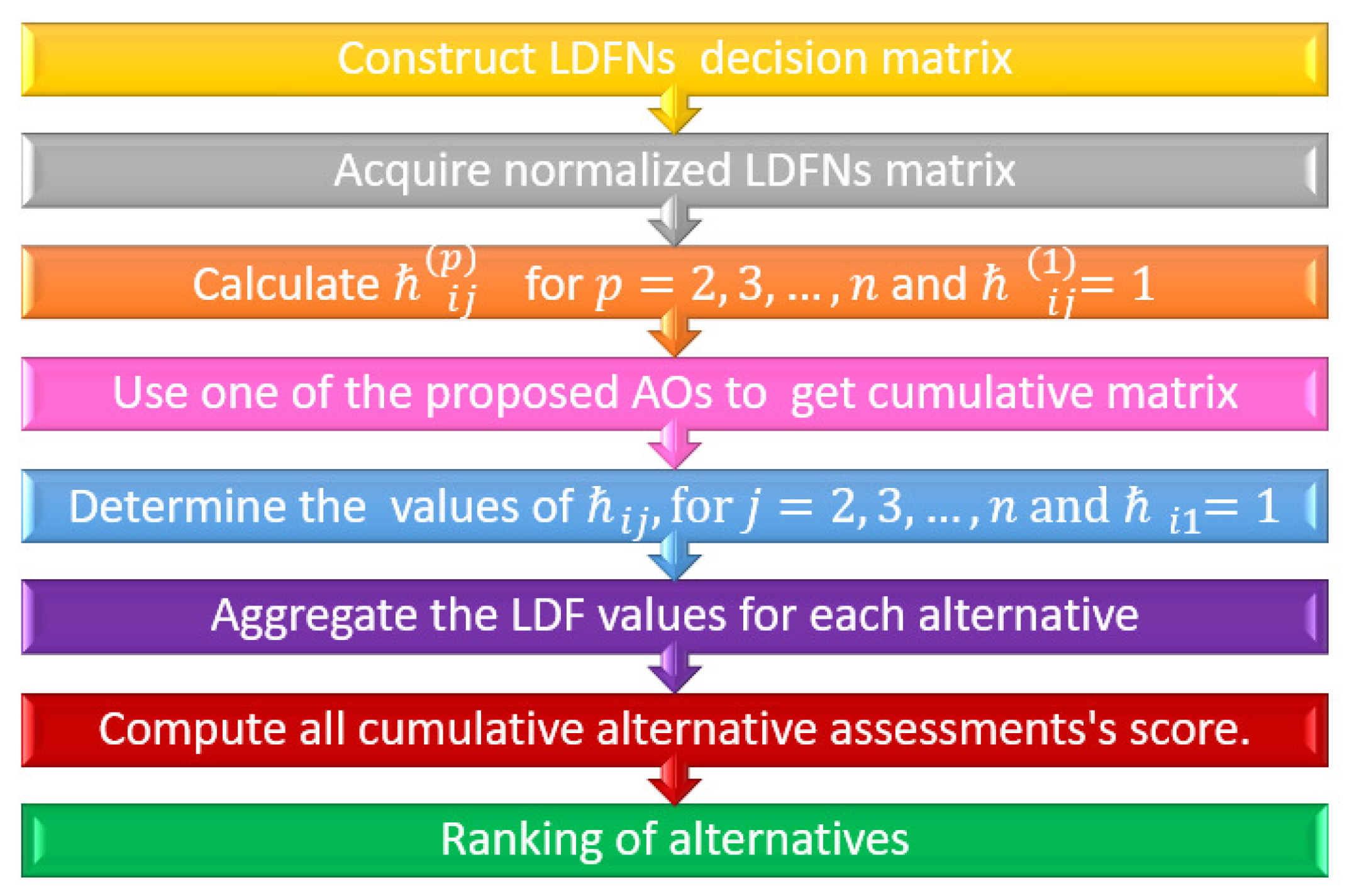
4. Proposed Methodology

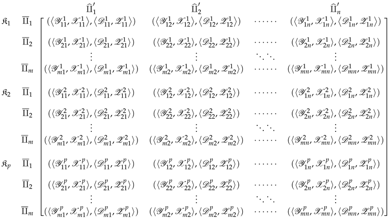
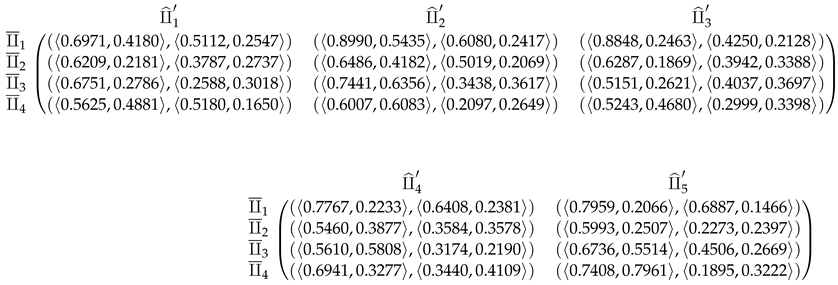
Let $\overline{⨿}=\{{\overline{⨿}}_1,{\overline{⨿}}_2,\dots ,{\overline{⨿}}_m\}$ be the assemblage of alternatives and ${\widehat{⨿}}^{\prime }=\{{\widehat{⨿}}_1^{\prime },{\widehat{⨿}}_2^{\prime },\dots ,{\widehat{⨿}}_n^{\prime }\}$ is the assemblage of criterion. Priorities are assigned between the criteria provided by the linear orientation in this case. ${\widehat{⨿}}_1^{\prime }\succ {\widehat{⨿}}_2^{\prime }\succ {\widehat{⨿}}_3^{\prime }\dots {\widehat{⨿}}_n^{\prime }$ indicates criteria ${\widehat{⨿}}_J^{\prime }$ has a high priority than ${\widehat{⨿}}_i^{\prime }$ if $j>i$. $\overline{{\rm Y}}=\{{\overline{{\rm Y}}}_1,{\overline{{\rm Y}}}_2,\dots ,{\overline{{\rm Y}}}_p\}$ is a assemblage of decision-makers (DM) and DMs are not given the same priority. Prioritization is provided by a linear pattern between the DMs given as, ${\overline{{\rm Y}}}_1\succ {\overline{{\rm Y}}}_2\succ {\overline{{\rm Y}}}_3\dots {\overline{{\rm Y}}}_p$ shows DM ${\overline{{\rm Y}}}_{\zeta }$ has a high importance than ${\overline{{\rm Y}}}_{\varrho }$ if $\zeta >\varrho$. DMs give a matrix according to their own standpoints $D^{\left(p\right)}={\left({\mathcal{B}}_{ij}^{\left(p\right)}\right)}_{m\times n}$, where ${\mathcal{B}}_{ij}^{\left(p\right)}$ is given for the alternatives ${\overline{⨿}}_i\in \overline{⨿}$ with respect to the attribute ${\widehat{⨿}}_j^{\prime }\in {\widehat{⨿}}^{\prime }$ by ${\overline{{\rm Y}}}_p$ DM. If all performance criteria are the same kind, there is no need for normalization; however, since MCGDM has two different types of evaluation criteria (benefit kind attributes ${\tau }_b$ and cost kinds attributes ${\tau }_c$), the matrix $D_{(}p)$ has been transformed into a normalize matrix using the normalization formula $Y^{\left(p\right)}={\left({\mathcal{P}}_{ij}^{\left(p\right)}\right)}_{m\times n,}$

$${\left({\mathcal{P}}_{ij}^{\left(p\right)}\right)}_{m\times n}=\left\{\begin{array}{cc}{\left({\mathcal{B}}_{ij}^{\left(p\right)}\right)}^c;\hfill & j\in {\tau }_c\hfill \\ {\mathcal{B}}_{ij}^{\left(p\right)};\hfill & j\in {\tau }_b.\hfill \end{array}\right.$$

(5)

where ${\left({\mathcal{B}}_{ij}^{\left(p\right)}\right)}^c$ show the compliment of ${\mathcal{B}}_{ij}^{\left(p\right)}$.

The suggested operators will be implemented to the MCGDM, which will require the preceding steps. Pictorial view of Algorithm is given in Figure 7.

Step 1:

Acquire a decision matrix $D^{\left(p\right)}={\left({\mathcal{B}}_{ij}^{\left(p\right)}\right)}_{m\times n}$ in the form of LDFNs from the decision makers.

Step 2:

Two kinds of criterion are described in the decision matrix: $\left({\tau }_c\right)$ cost type indicators and $\left({\tau }_b\right)$ benefit type indicators. There is no need for normalization if all indicators are of the same kind, but in MCGDM, there may be two types of criteria. The matrix was updated to the transforming response matrix in this case $Y^{\left(p\right)}={\left({\mathcal{P}}_{ij}^{\left(p\right)}\right)}_{m\times n}$ using the normalization formula given in Equation (5).

Step 3:

Calculate the values of ${\breve{\hslash }}_{ij}^{\left(p\right)}$ by following formula.

$${\breve{\hslash }}_{ij}^{\left(p\right)}={\overline{\prod }}_{k=1}^{p-1}\mathcal{H}\left({\mathcal{P}}_{ij}^{\left(k\right)}\right)(p=2\dots ,n),$$

(6)

$${\breve{\hslash }}_{ij}^{\left(1\right)}=1$$

Step 4:

${\mathcal{W}}_{ij}=\mathrm{LDFPWA}({\mathcal{P}}_{ij}^{\left(1\right)},{\mathcal{P}}_{ij}^{\left(2\right)},\dots {\mathcal{P}}_{ij}^{\left(p\right)})$

$$=\left(〈1-{\overline{\prod }}_{z=1}^p{(1-{\mathcal{Y}}_{ij}^z)}^{\frac{{\breve{\hslash }}_j^z}{{\gimel }_j{\breve{\hslash }}_j^z}},{\overline{\prod }}_{z=1}^p{\left({\mathcal{X}}_{ij}^z\right)}^{\frac{{\breve{\hslash }}_j^z}{{\gimel }_j{\breve{\hslash }}_j^z}}〉,〈1-{\overline{\prod }}_{z=1}^p{(1-{\mathcal{D}}_{ij}^z)}^{\frac{{\breve{\hslash }}_j^z}{{\gimel }_j{\breve{\hslash }}_j^z}},{\overline{\prod }}_{z=1}^p{\left({\mathcal{Z}}_{ij}^z\right)}^{\frac{{\breve{\hslash }}_j^z}{{\gimel }_j{\breve{\hslash }}_j^z}}〉\right)$$

(7)

or

${\mathcal{W}}_{ij}=\mathrm{LDFPWG}({\mathcal{P}}_{ij}^{\left(1\right)},{\mathcal{P}}_{ij}^{\left(2\right)},\dots {\mathcal{P}}_{ij}^{\left(p\right)})$

$$=\left(〈{\overline{\prod }}_{z=1}^p{\left({\mathcal{Y}}_{ij}^z\right)}^{\frac{{\breve{\hslash }}_j^z}{{\gimel }_j{\breve{\hslash }}_j^z}},1-{\overline{\prod }}_{z=1}^p{(1-{\mathcal{X}}_{ij}^z)}^{\frac{{\breve{\hslash }}_j^z}{{\gimel }_j{\breve{\hslash }}_j^z}}〉,〈{\overline{\prod }}_{z=1}^p{\left({\mathcal{D}}_{ij}^z\right)}^{\frac{{\breve{\hslash }}_j^z}{{\gimel }_j{\breve{\hslash }}_j^z}},1-{\overline{\prod }}_{z=1}^p{(1-{\mathcal{Z}}_{ij}^z)}^{\frac{{\breve{\hslash }}_j^z}{{\gimel }_j{\breve{\hslash }}_j^z}}〉\right)$$

(8)

Use one of the above mentioned AOs, to get one cumulative matrix $W^{\left(p\right)}={\left({\mathcal{W}}_{ij}\right)}_{m\times n}$ by aggregating all LDF decision matrices $Y^{\left(p\right)}={\left({\mathcal{P}}_{ij}^{\left(p\right)}\right)}_{m\times n}$.

Step 5:

Values of ${\breve{\hslash }}_{ij}$ determine by using given formula.

$${\breve{\hslash }}_{ij}={\overline{\prod }}_{k=1}^{j-1}\mathcal{H}\left({\mathcal{W}}_{ik}\right)(j=2\dots ,n),$$

(9)

$${\breve{\hslash }}_{i1}=1$$

Step 6:

Aggregate the LDF values ${\mathcal{W}}_{ij}$ for each alternative ${\overline{⨿}}_i$ by the LDFPWA (or LDFPWG) operator:

${\mathcal{W}}_i=\mathrm{LDFPWA}({\mathcal{P}}_{i1},{\mathcal{P}}_{i2},\dots {\mathcal{P}}_{in})$

$$=\left(〈1-{\overline{\prod }}_{j=1}^n{(1-{\mathcal{Y}}_j)}^{\frac{{\breve{\hslash }}_j}{{\gimel }_j{\breve{\hslash }}_j}},{\overline{\prod }}_{j=1}^n{\mathcal{X}}_j^{\frac{{\breve{\hslash }}_j}{{\gimel }_j{\breve{\hslash }}_j}}〉,〈1-{\overline{\prod }}_{j=1}^n{(1-{\mathcal{D}}_j)}^{\frac{{\breve{\hslash }}_j}{{\gimel }_j{\breve{\hslash }}_j}},{\overline{\prod }}_{j=1}^n{\mathcal{Z}}_j^{\frac{{\breve{\hslash }}_j}{{\gimel }_j{\breve{\hslash }}_j}}〉\right)$$

(10)

or

${\mathcal{W}}_i=\mathrm{LDFPWG}({\mathcal{P}}_{i1},{\mathcal{P}}_{i2},\dots {\mathcal{P}}_{in})$

$$=\left(〈{\overline{\prod }}_{j=1}^n{\mathcal{Y}}_j^{\frac{{\breve{\hslash }}_j}{{\gimel }_j{\breve{\hslash }}_j}},1-{\overline{\prod }}_{j=1}^n{(1-{\mathcal{X}}_j)}^{\frac{{\breve{\hslash }}_j}{{\gimel }_j{\breve{\hslash }}_j}}〉,〈{\overline{\prod }}_{j=1}^n{\mathcal{D}}_j^{\frac{{\breve{\hslash }}_j}{{\gimel }_j{\breve{\hslash }}_j}},1-{\overline{\prod }}_{j=1}^n{(1-{\mathcal{Z}}_j)}^{\frac{{\breve{\hslash }}_j}{{\gimel }_j{\breve{\hslash }}_j}}〉\right)$$

(11)

Step 7:

Compute all cumulative alternative assessment scores.

Step 8:

The alternatives were rated using the score feature, and the best option was chosen.

5. Case Study

RLs is described as the method of transporting things from their original point of origin to their final destination for purposes, such as value capture and re-use. Materials are transferred from vendors to end users through supply chain networks. The on-time delivery (OTD) metric is used by supply chain professionals to assess the efficacy of the flow. It is a fairly standard supply chain measurement that focuses on ensuring rapid and convenient delivery to the final user from the time the order is placed. However, the supply chain’s task does not end until the service reaches the end consumer. Customers return products for a variety of reasons, including purchasing the wrong item, receiving a faulty item, receiving an item that does not match the company’s logo and no longer needing the product. In such situations, you must plan for the return product’s shipment and refer it through different procedures like recycling, inspection, repairing, and dismantling. Many of these methods require the material to move backwards across the supply chain. There are many benefits of introducing RLs that benefit both customers and manufacturers. RLs is the procedure of restoring, reshaping, or recycling products that have reached the end of their useful lives. It could be used as an asset recovery tool for manufacturers, allowing them to derive as much value as possible from their products and obtain a second return on investment. Companies would benefit from RLs in the form of tax cuts and favorable media attention for doing their part to keep recycled products out of landfills. The single significant explanation for RLs is the increased value that businesses can see as a result of lower material costs. RLs have increased in importance since the start of the e-commerce era.

Shopping carts have also been supplanted in recent years by online retailers, with sales estimated to reach 414 million by 2018. Returns account for at least 30% of all products bought online, compared to 8.89% in traditional stores. This rapid rise in returned goods causes a lot of uncertainty in RLs, placing a lot of challenges on supply chains to effectively manage and implement logistics costs. As a result, you must meticulously plan and develop your reverse logistics. Metrics can be used to track reverse flow in your supply chain. The number of returns, product type and condition, dollar value, and amount of revenue returned are all included. An in-depth analysis of these indicators would help in the detection of problem areas, as well as the transformation of the risk of returns into an opportunity to develop the business. The benefits far outweigh the costs of implementing a reverse logistics strategy. Is the supply chain willing to take a step back?

RLs necessitates the same efficiencies as conventional “forward”logistics (customer support, storage, system integration, and so on). If you streamline the way goods pass back into the supply chain, you’ll see cost savings, happy consumers, and increased efficiency.

1. RLs provides a range of cost-cutting opportunities, ranging from lowering shipping prices to reselling products that would have been discarded if returned. Your profit margins will increase if money is reclaimed from recycled and resold materials and the rest of the system is running smoothly.

2. How your company handles returns can have a big effect on how customers view your brand. A defective product may be the source of a bad experience. It is as critical to deal with errors as it is to make sales. You must make things right if a consumer has a negative experience with some item. If you have choices for consumers who want to return products in a way that is convenient for them, it can go a long way toward increasing customer loyalty. These may include, among other things, a full refund regardless of the reason for the return, the right to return without the original receipt if returning to a physical store, and the ability to return without the original packaging.

3. Customer satisfaction would skyrocket if you had a streamlined system in place for consumers to quickly return goods and order replacements. It can also help to expedite the process of repairing, refurbishing, or reusing products, thus removing the need to purchase new ones.

4. RLs will help you find ways to reuse, resell, or recycle items that would otherwise end up in landfills. This raises the brand’s social and environmental obligations while still rising profit margins. By remanufacturing or refurbishing your products, you can extend their existence.

As a company grows, it faces new challenges, such as increased potential customers, new locations, revamped manufacturing processes, and other factors. Meeting such issues with capital and overhead spending is not always the most cost-effective option for some companies. It is also preferable for such companies to look beyond their systems to third-party service providers to provide the enhanced functionality that they need to continue expanding. This is where 3PRLPs come into play. 3PRLPs are a range of facilities and processes that an external agency offers to an organization for a variety of reasons, including cost reduction, increased efficiencies, and capability expansion. 3PRLP services are usually adaptable and flexible to meet the needs of individuals, which means they can be used on an as-needed or long-term basis, depending on the company’s goals and strategies. Businesses seek 3PRLP services for a variety of purposes. As a company grows, the demand for storage space often outstrips the company’s ability to meet it. 3PRLP warehouse management can be a viable option for businesses that are experiencing storage space issues. Other companies can face increasing shipping costs, as well as increased investments in infrastructure and automobiles. 3PRLPs vast fleets of specialized trucks and facilities are often a much more cost-effective choice. Then there are US businesses trying to expand into the Canadian market; a good 3PRLP will be able to help with many of the logistical challenges that these scenarios involve. Customer support, delivery times, refunds, order tracking, technical services, stock management, and other issues are just a few of the many reasons why businesses may choose to work with a 3PRLP. As you would expect, the more obstacles a company faces as it expands, the more value a 3PRLP associate can have. Supply chain experts are constantly striving to find new ways to improve efficiency, increase speed, and reduce logistics costs of which transportation typically makes up the largest component. Logistic cost breakdown is given in Figure 8.

The 3PRLP selection procedure involves a number of criteria; as a result, this shortlisting method can be viewed as an MCDM task. Present research on the 3PRLP selection issue indicates academic and industrial interest. A large number of MCDMs have been developed in recent years. Models were created in the context of the 3PRLP evaluation issue. Realistic RLs outsourcing assessments are often prepared in an imprecise and ambiguous setting due to a variety of factors, such as partial ignorance, imprecise assessment, and partial or unavailable decision-making for additional details [44]. The term “outsourcing” has been used in the American Glossary since at least 1981, when it was first used as “outside resourcing". Logistics outsourcing is one of a company’s biggest accomplishments. Nowadays, a logistics contract provider outsources many companies at the same time, resulting in the benefits of economic balance, which can assist the organization in lowering its costs. Despite these challenges, Yang et al. addressed how reduction in cost is rarely the primary goal of outsourcing in MCDM [45].

Numerous academics have outlined several modules of 3PRLP outsourcing:

(1)

the benefits and drawbacks of using a third-party logistics supplier [46];

(2)

evaluating and choosing 3PRLPs for long-term partnership [41].

The current research project focuses on the second module, which is concerned with the evaluation and selection of 3PRLPs in the decision-making process while considering sustainability perspectives. Adoption of 3PRLP is critical for maximizing the product cycle’s life span and returns, which aids in reducing environmental threats and addressing resource-related issues. According to reports, bureaucrats in developing countries have been encouraging and rendering sustainable development guidelines obligatory for the implementation of 3PRLP setups in SCM [47]. Many studies have been conducted to determine the best way to choose a 3PRLP from different perspectives [48,49,50]. Crisp values are seldom suitable for modeling such real-world decision-making situations. To deal with uncertain and ambiguous data, the Fuzzy set (FS) theory and its extensions have been widely used in real-world MCDM applications. In a Fuzzy world, Zarbakhshnia et al. [51] used the SWARA Fuzzy method to evaluate the requirements and COPRAS to grade 3PRLPs as sustainable. According to Liu et al. [52], the BWM should examine the array of 3PRLPs on IVPHFSs. Bai and Sarkis [53] pioneered a multi-method and multi-stage decision-making tool based on TOPSIS, VIKOR, and neighbourhood rough collection and Zarbakhshnia et al. recently developed a framework for evaluating 3PRLPs under FSs [54]. For determining the best S3PRLP for the automotive industry, Zhang and Su proposed model with dominance degree [55]. To assess and pick the best 3PRLPs, Efendigil et al. introduced a approach incorporating Fuzzy AHP and ANN [56]. Furthermore, Cheng and Lee used the ANP technique to choose 3PRLP for high-tech manufacturing [57]. Ho et al. recently introduced a approach incorporating quality feature implementation and the Fuzzy AHP to evaluate and pick the best 3PRLPs [58]. Chai et al. gave a comprehensive literature review on 3PRLPs [59].

Several researchers have spent the last two decades seeking to identify the critical requirements for analyzing and selecting 3PRLP. The researchers typically employed survey methodology to capture the key factors. In this article, we use the five criterion for selecting best 3PRLP given in

Table 2. Criterion and their references.

Criteria	Literature	Nature
Cost (${\widehat{⨿}}_1^{\prime }$)	Govindan et al. [60], Boyson et al. [61], Langley et al. [62]	Non-beneficial
	Meade and Sarkis [63], Gunasekaran et al. [64], Efendigil et al. [56]
	Stock et al. [65], Ha and Krishnan [66]
Experience (${\widehat{⨿}}_2^{\prime }$)	Ha and Krishnan [66], Amin and Zhang [67], Darvish et al. [68],	Beneficial
	Amin and Razmi [69], Saen [44], Chen [70]
Quality (${\widehat{⨿}}_3^{\prime }$)	Govindan et al. [60], Boyson et al. [61], Stock et al. [65],
	Saen [44], Mavi et al. [71], Li et al. [72]	Beneficial
Eco-design	Kuo et al. [73], Amindoust et al. [74], Shen et al. [75]	Beneficial
production (${\widehat{⨿}}_4^{\prime }$)	Govindan et al. [76], Kannan et al. [77], Jabbour et al. [78]
Reputation (${\widehat{⨿}}_5^{\prime }$)	Saen [44], Mavi et al. [71], Kannan et al. [79], Sen et al. [80]	Beneficial

, references regarding these five criteria also given.

5.1. Numerical Example

Consider a set of alternatives $\overline{⨿}=\{{\overline{⨿}}_1,{\overline{⨿}}_2,{\overline{⨿}}_3,{\overline{⨿}}_4\}$ and a set of criterion ${\widehat{⨿}}^{\prime }=\{{\widehat{⨿}}_1^{\prime },{\widehat{⨿}}_2^{\prime },{\widehat{⨿}}_3^{\prime },{\widehat{⨿}}_4^{\prime },{\widehat{⨿}}_5^{\prime }\}$, where

${\widehat{⨿}}_1^{\prime }$= cost,

${\widehat{⨿}}_2^{\prime }$= experience,

${\widehat{⨿}}_3^{\prime }$= quality,

${\widehat{⨿}}_4^{\prime }$= eco-design production,

${\widehat{⨿}}_5^{\prime }$= reputation.

Priorities are assigned among the criterion provided by the linear orientation. That is, ${\widehat{⨿}}_1^{\prime }\succ {\widehat{⨿}}_2^{\prime }\succ {\widehat{⨿}}_3^{\prime }\succ {\widehat{⨿}}_4^{\prime }\succ {\widehat{⨿}}_5^{\prime }$ indicates that the criterion are linearly ordered such that ${\widehat{⨿}}_j^{\prime }$ has a high priority than ${\widehat{⨿}}_i^{\prime }$ if $j>i$.

In this example, we use LDFNs as input data for ranking the given alternatives under the given attributes. Here three DMs are involved, i.e., $\overline{{{\rm Y}}_1},\overline{{{\rm Y}}_2}$ and $\overline{{{\rm Y}}_3}$. DMs are not given the same priority. Prioritization is provided by a linear pattern between the DMs given as, ${\overline{{\rm Y}}}_1\succ {\overline{{\rm Y}}}_2\succ {\overline{{\rm Y}}}_3$ shows DM ${\overline{{\rm Y}}}_{\zeta }$ has a high importance than ${\overline{{\rm Y}}}_{\varrho }$ if $\zeta >\varrho$.

Step 1:

Acquire a decision matrix $D^{\left(p\right)}={\left({\mathcal{B}}_{ij}^{\left(p\right)}\right)}_{m\times n}$ in the form of LDFNs from the decision makers, given in

Table 3. LDF decision matrix from ${\mathfrak{K}}_1$.

	${\widehat{⨿}}_1^{\prime }$	${\widehat{⨿}}_2^{\prime }$	${\widehat{⨿}}_3^{\prime }$	${\widehat{⨿}}_4^{\prime }$	${\widehat{⨿}}_5^{\prime }$
${\overline{⨿}}_1$	$(\langle 0.20,0.85\rangle ,\langle 0.15,0.65\rangle )$	$(\langle 0.95,0.55\rangle ,\langle 0.75,0.15\rangle )$	$(\langle 0.85,0.10\rangle ,\langle 0.50,0.10\rangle )$	$(\langle 0.75,0.25\rangle ,\langle 0.60,0.10\rangle )$	$(\langle 0.85,0.20\rangle ,\langle 0.80,0.10\rangle )$
${\overline{⨿}}_2$	$(\langle 0.10,0.70\rangle ,\langle 0.25,0.35\rangle )$	$(\langle 0.60,0.45\rangle ,\langle 0.65,0.15\rangle )$	$(\langle 0.65,0.15\rangle ,\langle 0.30,0.30\rangle )$	$(\langle 0.55,0.35\rangle ,\langle 0.40,0.35\rangle )$	$(\langle 0.65,0.10\rangle ,\langle 0.15,0.25\rangle )$
${\overline{⨿}}_3$	$(\langle 0.20,0.65\rangle ,\langle 0.35,0.15\rangle )$	$(\langle 0.70,0.50\rangle ,\langle 0.30,0.40\rangle )$	$(\langle 0.50,0.20\rangle ,\langle 0.45,0.45\rangle )$	$(\langle 0.65,0.45\rangle ,\langle 0.25,0.25\rangle )$	$(\langle 0.75,0.60\rangle ,\langle 0.30,0.30\rangle )$
${\overline{⨿}}_4$	$(\langle 0.30,0.50\rangle ,\langle 0.15,0.60\rangle )$	$(\langle 0.60,0.55\rangle ,\langle 0.15,0.15\rangle )$	$(\langle 0.65,0.35\rangle ,\langle 0.20,0.30\rangle )$	$(\langle 0.85,0.15\rangle ,\langle 0.40,0.40\rangle )$	$(\langle 0.85,0.95\rangle ,\langle 0.10,0.30\rangle )$

,

Table 4. LDF decision matrix from ${\mathfrak{K}}_2$.

	${\widehat{⨿}}_1^{\prime }$	${\widehat{⨿}}_2^{\prime }$	${\widehat{⨿}}_3^{\prime }$	${\widehat{⨿}}_4^{\prime }$	${\widehat{⨿}}_5^{\prime }$
${\overline{⨿}}_1$	$(\langle 0.85,0.45\rangle ,\langle 0.40,0.35\rangle )$	$(\langle 0.85,0.75\rangle ,\langle 0.25,0.45\rangle )$	$(\langle 0.95,0.85\rangle ,\langle 0.35,0.65\rangle )$	$(\langle 0.75,0.25\rangle ,\langle 0.80,0.65\rangle )$	$(\langle 0.70,0.25\rangle ,\langle 0.45,0.25\rangle )$
${\overline{⨿}}_2$	$(\langle 0.65,0.35\rangle ,\langle 0.30,0.45\rangle )$	$(\langle 0.65,0.50\rangle ,\langle 0.35,0.25\rangle )$	$(\langle 0.70,0.30\rangle ,\langle 0.35,0.55\rangle )$	$(\langle 0.65,0.35\rangle ,\langle 0.25,0.35\rangle )$	$(\langle 0.50,0.65\rangle ,\langle 0.35,0.20\rangle )$
${\overline{⨿}}_3$	$(\langle 0.25,0.75\rangle ,\langle 0.30,0.30\rangle )$	$(\langle 0.75,0.95\rangle ,\langle 0.25,0.45\rangle )$	$(\langle 0.65,0.25\rangle ,\langle 0.35,0.25\rangle )$	$(\langle 0.45,0.75\rangle ,\langle 0.45,0.25\rangle )$	$(\langle 0.60,0.35\rangle ,\langle 0.65,0.15\rangle )$
${\overline{⨿}}_4$	$(\langle 0.85,0.60\rangle ,\langle 0.20,0.45\rangle )$	$(\langle 0.65,0.70\rangle ,\langle 0.30,0.65\rangle )$	$(\langle 0.35,0.65\rangle ,\langle 0.45,0.45\rangle )$	$(\langle 0.30,0.85\rangle ,\langle 0.30,0.40\rangle )$	$(\langle 0.30,0.70\rangle ,\langle 0.25,0.45\rangle )$

and

Table 5. LDF decision matrix from ${\mathfrak{K}}_3$.

	${\widehat{⨿}}_1^{\prime }$	${\widehat{⨿}}_2^{\prime }$	${\widehat{⨿}}_3^{\prime }$	${\widehat{⨿}}_4^{\prime }$	${\widehat{⨿}}_5^{\prime }$
${\overline{⨿}}_1$	$(\langle 0.75,0.35\rangle ,\langle 0.45,0.30\rangle )$	$(\langle 0.65,0.25\rangle ,\langle 0.65,0.20\rangle )$	$(\langle 0.65,0.20\rangle ,\langle 035.,0.15\rangle )$	$(\langle 0.85,0.15\rangle ,\langle 0.30,0.30\rangle )$	$(\langle 0.65,0.15\rangle ,\langle 0.35,0.25\rangle )$
${\overline{⨿}}_2$	$(\langle 0.25,0.75\rangle ,\langle 0.30,0.30\rangle )$	$(\langle 0.75,0.25\rangle ,\langle 0.20,0.35\rangle )$	$(\langle 0.35,0.15\rangle ,\langle 0.65,0.20\rangle )$	$(\langle 0.25,0.65\rangle ,\langle 0.40,0.40\rangle )$	$(\langle 0.60,0.75\rangle ,\langle 0.20,0.30\rangle )$
${\overline{⨿}}_3$	$(\langle 0.85,0.60\rangle ,\langle 0.20,0.45\rangle )$	$(\langle 0.60,0.80\rangle ,\langle 0.50,0.30\rangle )$	$(\langle 0.25,0.60\rangle ,\langle 0.35,0.40\rangle )$	$(\langle 0.35,0.90\rangle ,\langle 0.25,0.10\rangle )$	$(\langle 0.50,0.85\rangle ,\langle 0.45,0.45\rangle )$
${\overline{⨿}}_4$	$(\langle 0.70,0.65\rangle ,\langle 0.15,0.35\rangle )$	$(\langle 0.45,0.70\rangle ,\langle 0.25,0.45\rangle )$	$(\langle 0.15,0.75\rangle ,\langle 0.30,0.30\rangle )$	$(\langle 0.40,0.60\rangle ,\langle 0.20,0.50\rangle )$	$(\langle 0.40,0.35\rangle ,\langle 0.50,0.20\rangle )$

.

Step 2:

Normalize the decision matrices acquired by DMs using Equation (5). There are two types of criterion. ${\widehat{⨿}}_1^{\prime }$ is cost type criteria and others are benefit type criterion, given in

Table 6. Normalized LDF decision matrix from ${\mathfrak{K}}_1$.

	${\widehat{⨿}}_1^{\prime }$	${\widehat{⨿}}_2^{\prime }$	${\widehat{⨿}}_3^{\prime }$	${\widehat{⨿}}_4^{\prime }$	${\widehat{⨿}}_5^{\prime }$
${\overline{⨿}}_1$	$(\langle 0.85,0.20\rangle ,\langle 0.65,0.15\rangle )$	$(\langle 0.95,0.55\rangle ,\langle 0.75,0.15\rangle )$	$(\langle 0.85,0.10\rangle ,\langle 0.50,0.10\rangle )$	$(\langle 0.75,0.25\rangle ,\langle 0.60,0.10\rangle )$	$(\langle 0.85,0.20\rangle ,\langle 0.80,0.10\rangle )$
${\overline{⨿}}_2$	$(\langle 0.70,0.10\rangle ,\langle 0.35,0.25\rangle )$	$(\langle 0.60,0.45\rangle ,\langle 0.65,0.15\rangle )$	$(\langle 0.65,0.15\rangle ,\langle 0.30,0.30\rangle )$	$(\langle 0.55,0.35\rangle ,\langle 0.40,0.35\rangle )$	$(\langle 0.65,0.10\rangle ,\langle 0.15,0.25\rangle )$
${\overline{⨿}}_3$	$(\langle 0.65,0.20\rangle ,\langle 0.15,0.35\rangle )$	$(\langle 0.70,0.50\rangle ,\langle 0.30,0.40\rangle )$	$(\langle 0.50,0.20\rangle ,\langle 0.45,0.45\rangle )$	$(\langle 0.65,0.45\rangle ,\langle 0.25,0.25\rangle )$	$(\langle 0.75,0.60\rangle ,\langle 0.30,0.30\rangle )$
${\overline{⨿}}_4$	$(\langle 0.50,0.30\rangle ,\langle 0.60,0.15\rangle )$	$(\langle 0.60,0.55\rangle ,\langle 0.15,0.15\rangle )$	$(\langle 0.65,0.35\rangle ,\langle 0.20,0.30\rangle )$	$(\langle 0.85,0.15\rangle ,\langle 0.40,0.40\rangle )$	$(\langle 0.85,0.95\rangle ,\langle 0.10,0.30\rangle )$

,

Table 7. Normalized LDF decision matrix from ${\mathfrak{K}}_2$.

	${\widehat{⨿}}_1^{\prime }$	${\widehat{⨿}}_2^{\prime }$	${\widehat{⨿}}_3^{\prime }$	${\widehat{⨿}}_4^{\prime }$	${\widehat{⨿}}_5^{\prime }$
${\overline{⨿}}_1$	$(\langle 0.45,0.85\rangle ,\langle 0.35,0.40\rangle )$	$(\langle 0.85,0.75\rangle ,\langle 0.25,0.45\rangle )$	$(\langle 0.95,0.85\rangle ,\langle 0.35,0.65\rangle )$	$(\langle 0.75,0.25\rangle ,\langle 0.80,0.65\rangle )$	$(\langle 0.70,0.25\rangle ,\langle 0.45,0.25\rangle )$
${\overline{⨿}}_2$	$(\langle 0.35,0.65\rangle ,\langle 0.45,0.30\rangle )$	$(\langle 0.65,0.50\rangle ,\langle 0.35,0.25\rangle )$	$(\langle 0.70,0.30\rangle ,\langle 0.35,0.55\rangle )$	$(\langle 0.65,0.35\rangle ,\langle 0.25,0.35\rangle )$	$(\langle 0.50,0.65\rangle ,\langle 0.35,0.20\rangle )$
${\overline{⨿}}_3$	$(\langle 0.75,0.25\rangle ,\langle 0.30,0.30\rangle )$	$(\langle 0.75,0.95\rangle ,\langle 0.25,0.45\rangle )$	$(\langle 0.65,0.25\rangle ,\langle 0.35,0.25\rangle )$	$(\langle 0.45,0.75\rangle ,\langle 0.45,0.25\rangle )$	$(\langle 0.60,0.35\rangle ,\langle 0.65,0.15\rangle )$
${\overline{⨿}}_4$	$(\langle 0.60,0.85\rangle ,\langle 0.45,0.20\rangle )$	$(\langle 0.65,0.70\rangle ,\langle 0.30,0.65\rangle )$	$(\langle 0.35,0.65\rangle ,\langle 0.45,0.45\rangle )$	$(\langle 0.30,0.85\rangle ,\langle 0.30,0.40\rangle )$	$(\langle 0.30,0.70\rangle ,\langle 0.25,0.45\rangle )$

and

Table 8. Normalized LDF decision matrix from ${\mathfrak{K}}_3$.

	${\widehat{⨿}}_1^{\prime }$	${\widehat{⨿}}_2^{\prime }$	${\widehat{⨿}}_3^{\prime }$	${\widehat{⨿}}_4^{\prime }$	${\widehat{⨿}}_5^{\prime }$
${\overline{⨿}}_1$	$(\langle 0.35,0.75\rangle ,\langle 0.30,0.45\rangle )$	$(\langle 0.65,0.25\rangle ,\langle 0.65,0.20\rangle )$	$(\langle 0.65,0.20\rangle ,\langle 0.35,0.15\rangle )$	$(\langle 0.85,0.15\rangle ,\langle 0.30,0.30\rangle )$	$(\langle 0.65,0.15\rangle ,\langle 0.35,0.25\rangle )$
${\overline{⨿}}_2$	$(\langle 0.75,0.25\rangle ,\langle 0.30,0.30\rangle )$	$(\langle 0.75,0.25\rangle ,\langle 0.20,0.35\rangle )$	$(\langle 0.35,0.15\rangle ,\langle 0.65,0.20\rangle )$	$(\langle 0.25,0.65\rangle ,\langle 0.40,0.40\rangle )$	$(\langle 0.60,0.75\rangle ,\langle 0.20,0.30\rangle )$
${\overline{⨿}}_3$	$(\langle 0.60,0.85\rangle ,\langle 0.45,0.20\rangle )$	$(\langle 0.60,0.80\rangle ,\langle 0.50,0.30\rangle )$	$(\langle 0.25,0.60\rangle ,\langle 0.35,0.40\rangle )$	$(\langle 0.35,0.90\rangle ,\langle 0.25,0.10\rangle )$	$(\langle 0.50,0.85\rangle ,\langle 0.45,0.45\rangle )$
${\overline{⨿}}_4$	$(\langle 0.65,0.70\rangle ,\langle 0.35,0.15\rangle )$	$(\langle 0.45,0.70\rangle ,\langle 0.25,0.45\rangle )$	$(\langle 0.15,0.75\rangle ,\langle 0.30,0.30\rangle )$	$(\langle 0.40,0.60\rangle ,\langle 0.20,0.50\rangle )$	$(\langle 0.40,0.35\rangle ,\langle 0.50,0.20\rangle )$

.

Step 3:

Calculate the values of ${\breve{\hslash }}_{ij}^{\left(p\right)}$ by Equation (6).

$${\breve{\hslash }}_{ij}^{\left(1\right)}=\left(\begin{array}{ccccc}1& 1& 1& 1& 1\\ 1& 1& 1& 1& 1\\ 1& 1& 1& 1& 1\\ 1& 1& 1& 1& 1\end{array}\right)$$

$${\breve{\hslash }}_{ij}^{\left(2\right)}=\left(\begin{array}{ccccc}0.7875& 0.7500& 0.7875& 0.7500& 0.8375\\ 0.6750& 0.6625& 0.6250& 0.5625& 0.6125\\ 0.5625& 0.5250& 0.5750& 0.5500& 0.5375\\ 0.6625& 0.5125& 0.5500& 0.6750& 0.4250\end{array}\right)$$

$${\breve{\hslash }}_{ij}^{\left(3\right)}=\left(\begin{array}{ccccc}0.3052& 0.3263& 0.3544& 0.4969& 0.5548\\ 0.3122& 0.3727& 0.3438& 0.3094& 0.3063\\ 0.3516& 0.2100& 0.3594& 0.2613& 0.3695\\ 0.3313& 0.2050& 0.2338& 0.2278& 0.1488\end{array}\right)$$

Step 4:

Use LDFPWA to aggregate all individual LDF decision matrices $Y^{\left(p\right)}={\left({\mathcal{P}}_{ij}^{\left(p\right)}\right)}_{m\times n}$ into one cumulative assessments matrix of the alternatives $W^{\left(p\right)}={\left({\mathcal{W}}_{ij}\right)}_{m\times n}$ using Equation (7) given below.

Step 5:

Evaluate the values of ${\breve{\hslash }}_{ij}$ by using Equation (9).

$${\breve{\hslash }}_{ij}=\left(\begin{array}{ccccc}1& 0.6339& 0.4314& 0.3074& 0.2272\\ 1& 0.6269& 0.3958& 0.2471& 0.1334\\ 1& 0.5884& 0.3076& 0.1759& 0.0914\\ 1& 0.6068& 0.2939& 0.1481& 0.0852\end{array}\right)$$

Step 6:

Aggregate the LDF values ${\mathcal{W}}_{ij}$ for each alternative ${\overline{⨿}}_i$ by the LDFPWA operator using Equation (10) given in

Table 9. LDF Aggregated values ${\mathcal{W}}_i$.

${\mathcal{W}}_1$	$(\langle 0.8160,0.3564\rangle ,\langle 0.5589,0.2308\rangle )$
${\mathcal{W}}_2$	$(\langle 0.6354,0.2694\rangle ,\langle 0.4069,0.2589\rangle )$
${\mathcal{W}}_3$	$(\langle 0.6696,0.3777\rangle ,\langle 0.3181,0.3163\rangle )$
${\mathcal{W}}_4$	$(\langle 0.5880,0.5125\rangle ,\langle 0.3908,0.2282\rangle )$

.

Step 7:

Calculate the score of all LDF aggregated values ${\mathcal{W}}_i$.

$$\mathcal{H}\left({\mathcal{W}}_1\right)=0.6969$$

$$\mathcal{H}\left({\mathcal{W}}_2\right)=0.6259$$

$$\mathcal{H}\left({\mathcal{W}}_3\right)=0.5735$$

$$\mathcal{H}\left({\mathcal{W}}_4\right)=0.5595$$

Step 8:

Rank by score function values.

$${\mathcal{W}}_1\succ {\mathcal{W}}_2\succ {\mathcal{W}}_3\succ {\mathcal{W}}_4$$

So,

$${\overline{⨿}}_1\succ {\overline{⨿}}_2\succ {\overline{⨿}}_3\succ {\overline{⨿}}_4$$

Bar chart for ranking of alternatives is given in Figure 9.

5.2. Comparative Analysis

In this section, we compare proposed AOs with some existing AOs. The uniqueness of our proposed operators is that they both yield the same result. We equate our results by solving the information data with some pre-existing operators and arriving at the same optimal decision. This demonstrates the robustness and validity of our proposed models. Because of their reference parameterizations, the presented techniques on LDFNs are more effective and superior to some existing theories. The beauty of this structure is that it creates an independence between MD and NMDs and creates categorization criteria due to parameterizations.

Table 10. Symmetry of ranking and optimal decision.

Authors	AOs	Ranking of Alternatives	The Optimal Alternative
Wang and Liu  [12]	IFEWA	${\overline{⨿}}_1\succ {\overline{⨿}}_4\succ {\overline{⨿}}_3\succ {\overline{⨿}}_2$	${\overline{⨿}}_1$
	IFEOWA	${\overline{⨿}}_1\succ {\overline{⨿}}_2\succ {\overline{⨿}}_4\succ {\overline{⨿}}_3$	${\overline{⨿}}_1$
Xu [9]	IFWA	${\overline{⨿}}_1\succ {\overline{⨿}}_2\succ {\overline{⨿}}_3\succ {\overline{⨿}}_4$	${\overline{⨿}}_1$
	IFOWA	${\overline{⨿}}_1\succ {\overline{⨿}}_2\succ {\overline{⨿}}_3\succ {\overline{⨿}}_4$	${\overline{⨿}}_1$
	IFHA	${\overline{⨿}}_1\succ {\overline{⨿}}_3\succ {\overline{⨿}}_2\succ {\overline{⨿}}_4$	${\overline{⨿}}_1$
Xu and Yager [10]	IFWG	${\overline{⨿}}_1\succ {\overline{⨿}}_2\succ {\overline{⨿}}_3\succ {\overline{⨿}}_4$	${\overline{⨿}}_1$
	IFOWG	${\overline{⨿}}_1\succ {\overline{⨿}}_3\succ {\overline{⨿}}_2\succ {\overline{⨿}}_4$	${\overline{⨿}}_1$
	IFHG	${\overline{⨿}}_1\succ {\overline{⨿}}_2\succ {\overline{⨿}}_4\succ {\overline{⨿}}_3$	${\overline{⨿}}_1$
Xu [81]	IFBM	${\overline{⨿}}_1\succ {\overline{⨿}}_2\succ {\overline{⨿}}_3\succ {\overline{⨿}}_4$	${\overline{⨿}}_1$
	WIFBM	${\overline{⨿}}_1\succ {\overline{⨿}}_4\succ {\overline{⨿}}_3\succ {\overline{⨿}}_2$	${\overline{⨿}}_1$
Zhao et al. [14]	GIFWA	${\overline{⨿}}_1\succ {\overline{⨿}}_2\succ {\overline{⨿}}_3\succ {\overline{⨿}}_4$	${\overline{⨿}}_1$
	GIFOWA	${\overline{⨿}}_1\succ {\overline{⨿}}_2\succ {\overline{⨿}}_3\succ {\overline{⨿}}_4$	${\overline{⨿}}_1$
Xu and Xia [82]	IGIFCA	${\overline{⨿}}_1\succ {\overline{⨿}}_2\succ {\overline{⨿}}_3\succ {\overline{⨿}}_4$	${\overline{⨿}}_1$
	BSI-GIFOA	${\overline{⨿}}_1\succ {\overline{⨿}}_4\succ {\overline{⨿}}_2\succ {\overline{⨿}}_3$	${\overline{⨿}}_1$
Proposed	LDFEWA	${\overline{⨿}}_1\succ {\overline{⨿}}_2\succ {\overline{⨿}}_3\succ {\overline{⨿}}_4$	${\overline{⨿}}_1$
	LDFEWG	${\overline{⨿}}_1\succ {\overline{⨿}}_2\succ {\overline{⨿}}_3\succ {\overline{⨿}}_4$	${\overline{⨿}}_1$

shows the symmetry of ranking and optimal decision as a comparison comparative analysis of proposed approach with previous approaches.

(i) LDFS outperforms other current theories such as Fuzzy set, IFS, PFS, and q-ROFS.

(ii) There are several real-world problems that are not addressed by other theories, and LDFS offered a wider evaluation space to address this.

(iii) Other aggregation operators proposed in the literature fail to aggregate linear Diophantine Fuzzy information, whereas our proposed aggregation operators are related to LDFSs. We obtain ${\overline{⨿}}_1\succ {\overline{⨿}}_2\succ {\overline{⨿}}_3\succ {\overline{⨿}}_4$ rating by our proposed aggregation operators; to validate our optimal option, we run this problem through other existing operators by converting LDF data into IFSs. The validity of our suggested aggregation operators is demonstrated by the fact that we obtain the same optimal decision.

6. Conclusions and Future Studies

Aggregation operators play an important role in information fusion for the real-life problems. A linear Diophantine Fuzzy information is new concept for modeling uncertainty in decision-making problems due the addition of reference parameters with membership and non-membership grades. First, we introduced new aggregation operators for modeling uncertainty by using linear Diophantine Fuzzy information. For this aim we developed new aggregation operators (AO) namely, “linear Diophantine Fuzzy prioritized weighted average” (LDFPWA) operator and “linear Diophantine Fuzzy prioritized weighted geometric”(LDFPWG) operator. Then we proposed certain essential properties of new prioritized AOs. Secondly, we discussed a practical application of third party reverse logistic provider (3PRLP) optimization problem. A numerical example to discuss 3PRLP is presented to discuss the efficiency, superiority, and rationality of the proposed approach. A comparative analysis is presented to discuss the symmetry of optimal decision and ranking of feasible alternatives.

References

1. Zadeh, L.A. Fuzzy sets. Inf. Control 1965, 8, 338–353. [Google Scholar] [CrossRef] [Green Version]
2. Atanassov, K.T. Intuitionistic fuzzy sets. Fuzzy Sets Syst. 1986, 20, 87–96. [Google Scholar] [CrossRef]
3. Atanassov, K.T. Geometrical interpretation of the elemets of the intuitionistic fuzzy objects. Int. J. Bioautom. 1986, 20 (Suppl. 1), S27–S42. [Google Scholar]
4. Yager, R.R.; Abbasov, A.M. Pythagorean membership grades, complex numbers, and decision making. Int. J. Intell. Syst. 2013, 28, 436–452. [Google Scholar] [CrossRef]
5. Yager, R.R. Pythagorean fuzzy subsets. In Proceedings of the IFSA World Congress and NAFIPS Annual Meeting (IFSA/NAFIPS), Edmonton, AB, Canada, 24–28 June 2013; pp. 57–61. [Google Scholar]
6. Yager, R.R. Pythagorean membership grades in multi criteria decision-making. IEEE Trans. Fuzzy Syst. 2014, 22, 958–965. [Google Scholar] [CrossRef]
7. Yager, R.R. Generalized orthopair fuzzy sets. IEEE Trans. Fuzzy Syst. 2017, 25, 1222–1230. [Google Scholar] [CrossRef]
8. Alcantud, J.C.R.; Garcia, G.S. A new criterion for soft set based decision making problems under incomplete information. Int. J. Comput. Intell. Syst. 2017, 10, 394–404. [Google Scholar] [CrossRef] [Green Version]
9. Xu, Z.S. Intuitionistic fuzzy aggregation operators. IEEE Transections Fuzzy Syst. 2007, 15, 1179–1187. [Google Scholar]
10. Xu, Z.S.; Yager, R.R. Some geometric aggregation operators based on intuitionistic fuzzy sets. Int. J. Gen. Syst. 2006, 35, 417–433. [Google Scholar] [CrossRef]
11. Hashmi, M.R.; Riaz, M.; Smarandache, F. m-polar Neutrosophic Topology with Applications to Multi-Criteria Decision-Making in Medical Diagnosis and Clustering Analysis. Int. J. Fuzzy Syst. 2020, 22, 273–292. [Google Scholar] [CrossRef]
12. Wang, W.; Liu, X. Intuitionistic fuzzy information aggregation using Einstein operators. IEEE Transections Fuzzy Syst. 2012, 20, 923–938. [Google Scholar] [CrossRef]
13. Zhang, H.Y.; Wang, J.Q.; Chen, X.H. Interval neutrosophic sets and their applications in multi-criteria decision making problems. Sci. World J. 2014, 2014, 645953. [Google Scholar]
14. Zhao, H.; Xu, Z.S.; Ni, M.F.; Lui, S.S. Generalized aggregation operators for intuitionistic fuzzy sets. Int. J. Intell. Syst. 2010, 25, 1–30. [Google Scholar] [CrossRef]
15. Garg, H. A new generalized Pythagorean fuzzy information aggregation using Einstein operators and its applications to decision-making. Int. J. Intell. Syst. 2016, 31, 886–920. [Google Scholar] [CrossRef]
16. Mahmood, T.; Ullah, K.; Khan, Q.; Jan, N. An approach toward decision-making and medical diagnosis problems using the concept of spherical fuzzy sets. Neural Comput. Appl. 2019, 31, 7041–7053. [Google Scholar] [CrossRef]
17. Feng, F.; Liang, M.; Fujita, H.; Yager, R.R.; Liu, X. Lexicographic orders of intuitionistic fuzzy values and their relationships. Mathematics 2019, 7, 1–7. [Google Scholar] [CrossRef] [Green Version]
18. Akram, M.; Yaqoob, N.; Ali, G.; Chammam, W. Extensions of Dombi aggregation operators for decision making under m-polar fuzzy information. J. Math. 2020, 6, 1–20. [Google Scholar] [CrossRef]
19. Akram, M.; Shahzadi, G.; Peng, X. Extension of Einstein Geometric Operators to Multi-Attribute Decision Making under q-Rung Orthopair Fuzzy Information. Available online: https://link.springer.com/article/10.1007 (accessed on 20 May 2021).
20. Peng, X.D.; Yang, Y. Some results for Pythagorean fuzzy sets. Int. J. Intell. Syst. 2015, 30, 1133–1160. [Google Scholar] [CrossRef]
21. Zhang, X.L.; Xu, Z.S. Extension of TOPSIS to multiple criteria decision making with Pythagorean fuzzy sets. Int. J. Intell. Syst. 2014, 29, 1061–1078. [Google Scholar] [CrossRef]
22. Karaaslan, F.; Ozlu, S. Correlation coefficients of dual type-2 hesitant fuzzy sets and their applications in clustering analysis. Int. J. Intell. Syst. 2020, 35, 1200–1229. [Google Scholar] [CrossRef]
23. Sitara, M.; Akram, M.; Riaz, M. Decision-making analysis based on q-rung picture fuzzy graph structures. J. Appl. Math. Comput. 2021. [Google Scholar] [CrossRef]
24. Riaz, M.; Hashmi, M.R. Linear Diophantine fuzzy set and its applications towards multi-attribute decision making problems. J. Intell. Fuzzy Syst. 2019, 37, 5417–5439. [Google Scholar] [CrossRef]
25. Kamaci, H. Linear Diophantine fuzzy algebraic structures. J. Ambient. Intell. Humaniz. Comput. 2021. [Google Scholar] [CrossRef]
26. Ayub, S.; Shabir, M.; Riaz, M.; Aslam, M.; Chinram, R. Linear Diophantine fuzzy relations and their algebraic properties with decision making. Symmetry 2021, 13, 945. [Google Scholar] [CrossRef]
27. Almagrabi, A.O.; Abdullah, S.; Shams, M. A new approach to q-linear Diophantine fuzzy emergency decision support system for COVID19. J. Ambient. Intell. Humanoized Comput. 2021. [Google Scholar] [CrossRef]
28. Pamucar, D. Normalized weighted Geometric Dombi Bonferoni Mean Operator with interval grey numbers: Application in multicriteria decision making. Rep. Mech. Eng. 2020, 1, 44–52. [Google Scholar] [CrossRef]
29. Pamucar, D.; Jankovic, A. The application of the hybrid interval rough weighted Power-Heronian operator in multi-criteria decision making. Oper. Res. Eng. Sci. Theory Appl. 2020, 3, 54–73. [Google Scholar] [CrossRef]
30. Riaz, M.; Salabun, W.; Farid, H.M.A.; Ali, N.; Watróbski, J. A robust q-rung orthopair fuzzy information aggregation using Einstein operations with application to sustainable energy planning decision management. Energies 2020, 13, 2125. [Google Scholar] [CrossRef]
31. Riaz, M.; Pamucar, D.; Farid, H.M.A.; Hashmi, M.R. q-Rung Orthopair Fuzzy Prioritized Aggregation Operators and Their Application Green Supplier Chain Management. Symmetry 2020, 12, 976. [Google Scholar] [CrossRef]
32. Riaz, M.; Farid, H.M.A.; Karaaslan, F.; Hashmi, M.R. Some q-rung orthopair fuzzy hybrid aggregation operators and TOPSIS method for multi-attribute decision-making. J. Intell. Fuzzy Syst. 2020, 39, 1227–1241. [Google Scholar] [CrossRef]
33. Riaz, M.; Farid, H.M.A.; Kalsoom, H.; Pamucar, D.; Chu, Y.M. A Robust q-rung orthopair fuzzy Einstein prioritized aggregation operators with application towards MCGDM. Symmetry 2020, 12, 1058. [Google Scholar] [CrossRef]
34. Riaz, M.; Garg, H.; Farid, H.M.A.; Chinram, R. Multi-criteria decision making based on bipolar picture fuzzy operators and new distance measures. Comput. Model. Eng. Sci. 2021, 127, 771–800. [Google Scholar] [CrossRef]
35. Yager, R.R. Prioritized aggregation operators. Int. J. Approx. Reason. 2008, 48, 263–274. [Google Scholar] [CrossRef] [Green Version]
36. Ali, Z.; Mahmood, T.; Ullah, K.; Khan, Q. Einstein Geometric Aggregation Operators using a Novel Complex Interval-valued Pythagorean Fuzzy Setting with Application in Green Supplier Chain Management. Rep. Mech. Eng. 2021, 2, 105–134. [Google Scholar] [CrossRef]
37. Ramakrishnan, K.R.; Chakraborty, S. A cloud TOPSIS model for green supplier selection. Facta Univ. Ser. Mech. Eng. 2020, 18, 375–397. [Google Scholar]
38. Petrovic, G.; Mihajlovic, J.; Cojbasic, Z.; Madic, M.; Marinkovic, D. Comparison of three fuzzy MCDM methods for solving the supplier selection problem. Facta Univ. Ser. Mech. Eng. 2019, 17, 455–469. [Google Scholar] [CrossRef]
39. Badi, I.; Pamucar, D. Supplier selection for steelmaking company by using combined Grey-MARCOS methods. Decis. Mak. Appl. Manag. Eng. 2020, 3, 37–48. [Google Scholar] [CrossRef]
40. Karamasa, C.; Demir, E.; Memis, S.; Korucuk, S. Weighting the factors affecting logistics outsourcing. Decis. Mak. Appl. Manag. Eng. 2021, 4, 19–32. [Google Scholar] [CrossRef]
41. Aguezzoul, A. Third-Party Logistics Selection Problem: A Literature Review on Criteria and Methods. Omega 2014, 49, 69–78. [Google Scholar] [CrossRef]
42. Prahinski, C.; Kocabasoglu, C. Empirical research opportunities in reverse supply chains. Omega 2006, 34, 519–532. [Google Scholar] [CrossRef]
43. Zareinejad, M.; Javanmard, H. Evaluation and selection of a third-party reverse logistics provider using ANP and IFG-MCDM methodology. Life Sci. J. 2013, 10, 350–355. [Google Scholar]
44. Saen, R.F. A new model for selecting third-party reverse logistics providers in the presence of multiple dual-role factors. Int. J. Adv. Manuf. Technol. 2010, 46, 405–410. [Google Scholar] [CrossRef] [Green Version]
45. Yang, D.H.; Kim, S.; Nam, C.; Min, J.W. Developing a decision model for business process outsourcing. Comput. Oper. Res. 2007, 34, 3769–3778. [Google Scholar] [CrossRef]
46. Hsiao, H.; Kemp, R.G.M.; der Vorst, J.G.A.V.; Omta, S.O. A classification of logistic outsourcing levels and their impact on service performance: Evidence from the food processing industry. Int. J. Prod. Econ. 2010, 124, 75–86. [Google Scholar] [CrossRef]
47. Jabbour, A.B.L.; Latan, C.J.C.; Teixeira, A.A.; Oliveira, J.H.C. Quality management, environmental management maturity, green supply chain practices and green performance of Brazilian companies with ISO 14001 certification: Direct and indirect effects. Transp. Res. Logist. Transp. Rev. 2014, 67, 39–51. [Google Scholar] [CrossRef]
48. Pamucar, D.; Chatterjee, K.; Zavadskas, E.K. Assessment of third-party logistics provider using multi-criteria decision-making approach based on interval rough numbers. Comput. Ind. Eng. 2019, 127, 383–407. [Google Scholar] [CrossRef]
49. Yayla, A.Y.; Oztekin, A.; Gumus, A.T.; Gunasekaran, A. A hybrid data analytic methodology for 3PL transportation provider evaluation using fuzzy multi-criteria decision making. Int. J. Prod. Res. 2015, 53, 6097–6113. [Google Scholar] [CrossRef]
50. Roy, J.; Adhikary, K.; Kar, S.; Pamucar, D. A rough strength relational DEMATEL model for analysing the key success factors of hospital service quality. Decis. Making Appl. Manag. Eng. 2018, 1, 121–142. [Google Scholar] [CrossRef]
51. Zarbakhshnia, N.; Soleimani, H.; Ghaderi, H. Sustainable thirdparty reverse logistics provider evaluation and selection using fuzzy SWARA and developed fuzzy COPRAS in the presence of risk criteria. Appl. Soft Comput. 2018, 65, 307–319. [Google Scholar] [CrossRef]
52. Liu, A.; Ji, X.; Lu, H.; Liu, H. The selection of 3PRLs on self-service mobile recycling machine: Interval-valued Pythagorean hesitant fuzzy best-worst multi-criteria group decision-making. J. Clean. Prod. 2019, 230, 734–750. [Google Scholar] [CrossRef]
53. Bai, C.; Sarkis, J. Integrating and extending data and decision tools for sustainable third-party reverse logistics provider selection. Oper. Res. Comput. 2019, 110, 188–207. [Google Scholar] [CrossRef]
54. Zarbakhshnia, N.; Wu, Y.; Govindan, K.; Soleimani, H. A novel hybrid multiple attribute decision-making approach for outsourcing sustainable reverse logistics. J. Clean. Prod. 2020, 242, 118461. [Google Scholar] [CrossRef]
55. Zhang, X.; Su, T. The dominance degree-based heterogeneous linguistic decision-making technique for sustainable S3PRLP selection. Complexity 2020, 2020, 6102036. [Google Scholar]
56. Efendigil, T.; Önüt, S.; Kongar, E. A Holistic Approach for Selecting a Third-Party Reverse Logistics Provider in the Presence of Vagueness. Comput. Ind. Eng. 2008, 54, 269–287. [Google Scholar] [CrossRef]
57. Cheng, Y.; Lee, F. Outsourcing Reverse Logistics of High-Tech Manufacturing Firms by using a Systematic Decision-Making Approach: TFT-LCD Sector in Taiwan. Ind. Mark. Manag. 2010, 39, 1111–1119. [Google Scholar] [CrossRef]
58. Ho, W.; He, T.; Lee, C.K.M. Emrouznejad, A. Strategic Logistics Outsourcing: An Integrated QFD and Fuzzy AHP Approach. Expert Syst. Appl. 2012, 39, 10841–10850. [Google Scholar] [CrossRef]
59. Chai, J.; Liu, J.N.; Ngai, E.W. Application of Decision-Making Techniques in Supplier Selection: A Systematic Review of Literature. Expert Syst. Appl. 2013, 40, 3872–3885. [Google Scholar] [CrossRef]
60. Govindan, K.; Pokharel, S.; Kumar, P.S. A hybrid approach using ISM and fuzzy TOPSIS for the selection of reverse logistics provider. Resour. Conserv. Recycl. 2009, 54, 28–36. [Google Scholar]
61. Boyson, S.; Corsi, T.; Dresner, M.; Rabinovich, E. Managing third party logistics relationships: What does it take. J. Bus. Logist. 1999, 20, 73–100. [Google Scholar]
62. Langley, C.J.; Allen, O.R.; Tyndall, O.R. Third-Party Logistics Study Results and Finding of the 2002 Seventh Annual Study; Georgia Institute of Technology: Atlanta, GA, USA, 2002; Unpublished Report. [Google Scholar]
63. Meade, L.; Sarkis, J. A conceptual model for selecting and evaluating third-party reverse logistics providers. Supply Chain. 2002, 7, 283–295. [Google Scholar] [CrossRef]
64. Gunasekaran, A.; Patel, C.; McGaughey, R.E. A framework for supply chain performance measurement. Int. J. Prod. Econ. 2004, 87, 333–347. [Google Scholar] [CrossRef]
65. Stock, O.N.; Oreis, N.P.; Kasarda, J.D. Logistics strategy and structure a conceptual framework. Int. J. Oper. Prod. Manag. 1998, 18, 37–52. [Google Scholar] [CrossRef]
66. Ha, S.H.; Krishnan, R. A hybrid approach to supplier selection for the maintenance of a competitive supply chain. Expert Syst. Appl. 2008, 34, 1303–1311. [Google Scholar] [CrossRef]
67. Amin, S.H.; Zhang, G. An integrated model for closed-loop supply chain configuration and supplier selection: Multi-objective approach. Expert Syst. Appl. 2012, 39, 6782–6791. [Google Scholar] [CrossRef]
68. Darvish, M.; Yasaei, M.; Saeedi, A. Application of graph theory and matrix methods for contractor ranking. Int. J. Proj. Manag. 2009, 27, 610–619. [Google Scholar] [CrossRef]
69. Amin, S.H.; Razmi, J. An integrated fuzzy model for supplier management: A case study of ISP selection and evaluation. Expert Syst. Appl. 2009, 36, 8639–8648. [Google Scholar] [CrossRef]
70. Chen, Y.J. Structured methodology for supplier selection and evaluation in a supply chain. Inf. Sci. 2011, 181, 1651–1670. [Google Scholar] [CrossRef]
71. Mavi, R.K.; Goh, M.; Zarbakhshnia, N. Sustainable third party reverse logistic provider selection with fuzzy SWARA and fuzzy MOORA in plastic industry. Int. J. Adv. Manuf. Technol. 2017, 91, 2401–2418. [Google Scholar] [CrossRef]
72. Li, Y.L.; Ying, C.S.; Chin, K.S.; Yang, H.T.; Xu, J. Third party reverse logistics provider selection approach based on hybrid-information MCDM and cumulative prospect theory. J. Clean. Prod. 2018, 195, 573–584. [Google Scholar] [CrossRef]
73. Kuo, R.J.; Wang, Y.C.; Tien, F.C. Integration of artificial neural network andMADA methods for green supplier selection. J. Clean. Prod. 2010, 18, 1161–1170. [Google Scholar] [CrossRef]
74. Amindoust, A.; Ahmed, S.; Saghafinia, A.; Bahreininejad, A. Sustainable supplier selection: A ranking model based on fuzzy inference system. Appl. Soft Comput. 2012, 12, 1668–1677. [Google Scholar] [CrossRef]
75. Shen, L.; Olfat, L.; Govindan, K.; Khodaverdi, R.; Diabatd, A. A fuzzy multi criteria approach for evaluating green supplier’s performance in green supply chain with linguistic preferences. Resour. Conserv. Recycl. 2013, 74, 170–179. [Google Scholar] [CrossRef]
76. Govindan, K.; Khodaverdi, R.; Jafarian, A. A fuzzy multi criteria approach for measuring sustainability performance of a supplier based on triple bottom line approach. J. Clean. Prod. 2013, 47, 345–354. [Google Scholar] [CrossRef]
77. Kannan, D.; Khodaverdi, R.; Olfat, L.; Jafarian, A.; Diabat, A. Integrated fuzzy multi criteria decision making method and multiobjective programming approach for supplier selection and order allocation in a green supply chain. J. Clean. Prod. 2013, 47, 355–366. [Google Scholar] [CrossRef]
78. Jabbour, A.B.; Jabbour, C.; Govindan, K.; Kannan, D.; Arantes, A.F. Mixed methodology to analyze the relationship between maturity of environmental management and the adoption of green supply chain management in Brazil. Resour. Conserv. Recycl. 2014, 92, 255–267. [Google Scholar] [CrossRef]
79. Kannan, D.; Garg, K.; Jha, P.C.; Diabat, A. Integrating disassembly line balancing in the planning of a reverse logistics network from the perspective of a third party provider. Ann. Oper. Res. 2017, 253, 353–376. [Google Scholar] [CrossRef]
80. Sen, D.K.; Datta, S.; Mahapatra, S.S. Decision support framework for selection of 3PL providers: Dominance-based approach in combination with grey set theory. Int. J. Inf. Technol. Decis. Mak. 2017, 16, 25–57. [Google Scholar] [CrossRef]
81. Xu, Z.S.; Yager, R.R. Intuitionistic Fuzzy Bonferroni Means. IEEE Trans. Syst. 2011, 41, 568–578. [Google Scholar]
82. Xu, Z.S.; Xia, M.M. Induced generalized intuitionistic fuzzy operators. Knowl. Based Syst. 2011, 24, 197–209. [Google Scholar] [CrossRef]
Figure 1. Graphical representation of valuation space of IFSs.
Symmetry 13 01152 g001
Figure 2. Graphical representation of valuation space of PFSs.
Symmetry 13 01152 g002
Figure 3. Graphical representation of valuation space of LDFSs.
Symmetry 13 01152 g003
Figure 4. LDFS with D , Z = 0.3 , 0.4 .
Symmetry 13 01152 g004
Figure 5. LDFS with D , Z = 0.8 , 0.1 .
Symmetry 13 01152 g005
Figure 6. LDFS with D , Z = 0.5 , 0.5 .
Symmetry 13 01152 g006
Figure 7. Pictorial view of Algorithm.
Symmetry 13 01152 g007
Figure 8. Logistic cost breakdown.
Symmetry 13 01152 g008
Figure 9. Bar chart for ranking of alternatives.
Symmetry 13 01152 g009