Exploring QED Effects to Diphoton Production at Hadron Colliders

Abstract

In this article, we report phenomenological studies about the impact of $\mathcal{O}\left(\alpha \right)$ corrections to diphoton production at hadron colliders. We explore the application of the Abelianized version of the $q_T$-subtraction method to efficiently compute NLO QED contributions, taking advantage of the symmetries relating QCD and QED corrections. We analyze the experimental consequences due to the selection criteria and we find percent-level deviations for $M_{\gamma \gamma }>1\mathrm{TeV}$. An accurate description of the tail of the invariant mass distribution is very important for new physics searches which have the diphoton process as one of their main backgrounds. Moreover, we emphasize the importance of properly dealing with the observable photons by reproducing the experimental conditions applied to the event reconstruction.

1. Introduction

Direct photon production in hadronic collisions provides an excellent opportunity to test Standard Model (SM) predictions and explore potential new physics effects, due to its very clean experimental signature. Photons are also very relevant to study the internal structure of colliding particles [1,2] because they can shed light on the parton level kinematics, leading to new interesting paths to unveil the hidden symmetries of nature.

In this phenomenological context, one process of special relevance is the production of a pair of prompt photons (i.e., diphoton production), which was one of the key channels for the discovery of a new particle compatible with the SM-Higgs boson [3,4]. This indicates that direct photon production might also play an important role in the precision physics program for future colliders [5,6,7,8,9,10,11,12,13].

Due to its relevance, the direct diphoton production has been extensively studied and its perturbative corrections were computed in several models. At the lowest order (LO), only the $q\overline{q}$ partonic channel is available. The first quantitative correction appears at the next-to-leading order (NLO) in the strong coupling constant ${\alpha }_{\mathrm{S}}$ [14,15,16,17], which includes the $qg$ channel and provides a noticeable enhancement due to the gluonic luminosity in the low-x region. At the next-to-next-to-leading order (NNLO) in ${\alpha }_{\mathrm{S}}$ (i.e., $\mathcal{O}\left({\alpha }_{\mathrm{S}}^2\right)$), the $gg$ channel becomes available. Its contribution is comparable to the Born cross-section, but the total NNLO correction is still dominated by the $qg$ channel. The NNLO QCD corrections were first calculated in Ref. [18] and later in Ref. [19]. The QCD resummed corrections have been recently obtained up to NNLL accuracy [20], thus improving the phenomenological description by including the effects due to low-energy gluon radiation. Recently, articles on diphoton production at NNLO were published, studying in detail the isolation criteria [21,22,23,24,25,26,27,28], the weight of the fragmentation component [21,22,24,26], the reliability of the prediction under symmetric cuts on single final photons [21], the scale sensitivity of the process and the hybrid isolation criteria [29,30], among other features of this important process. In addition, the diphoton background could be potentially interesting as an indirect measurement of the top-quark mass [31,32].

Besides the direct photon production from the hard subprocess, photons can be generated through the fragmentation mechanism, which involves non-perturbative transitions from QCD partons. The complete NLO single- and double-fragmentation contributions are implemented in DIPHOX [14]. The measured photon cross-sections use isolation prescriptions in order to reduce the large reducible background (associated to photons that are faked by jets or produced by hadron decays). Two of these prescriptions are the standard cone isolation and the smooth cone isolation [33] prescriptions. While measured cross-sections rely on the standard cone criterion, theoretical calculations can be greatly simplified with the smooth cone prescription. It is worth noticing that both algorithms produce similar results [22,34] for those isolation parameters implemented by the experiment.

Other important effect to be considered in the context of photon production is the presence of electroweak (EW) corrections. Leaving aside the large gluon luminosity at the LHC, a simple power counting shows that the NLO QED corrections could compete with the NNLO QCD contributions because ${\alpha }_{\mathrm{S}}^2\approx \alpha$. For this reason, the higher-order QED and EW effects deserve a serious treatment. Several studies about the EW corrections to gauge boson production [35,36,37,38,39,40] and diphoton production [41,42,43,44] showed small but still non-negligible contributions, which might play a crucial role in the context of the precision physics program. Moreover, we have explored the impact of pure QED and mixed QCD-QED corrections in the DGLAP equations [45,46,47] and we found that they could provide non-negligible effects to the PDF evolution. In particular, the NLO QED corrections to the diphoton production process are sensitive to the photon PDF through the $q\gamma$ channel, which might propagate the information related to this distribution to the final cross-section result.

From the point of view of new physics searches, the high-energy region of the diphoton spectrum could be used to impose constraints on many models. Since no new particles are predicted by the SM beyond the TeV scale, the inclusion of higher-order EW and QCD effects could only lead to an enhancement/decrease of the distributions without introducing any peak. Thus, a proper understanding of all the SM effects for this region might allow to impose tighter constraints to BSM models involving a continuum spectrum at high-energies (for instance, large extra-dimensions or Randall–Sundrum with composite fermions [48]).

The purpose of this article is to describe interesting phenomenological features of the NLO QED corrections to diphoton production, which might be useful for deeper studies of this process including higher-order mixed QCD-EW corrections. We start in Section 2 describing the theoretical framework used to perform the computation, centering the discussion in the different partonic channels contributing to the process. Special emphasis is put on the treatment of the electromagnetic coupling, because it leads to noticeable corrections to the theoretical predictions. Then, in Section 2.1, we explain the experimental cuts applied, focusing on the photon isolation and reconstruction algorithms. In Section 3, we present our predictions for LHC, highlighting the effects due to the ordering algorithms used to deal with the radiated photons. Besides that, we briefly comment about the implementation of a clustering (i.e., merging) algorithm for reconstructing the photons and the dependence of the results on the use of different PDF sets, and the photon PDF in particular. Finally, in Section 4 we present our conclusions and a brief discussion about the importance of higher-order QED corrections in future experiments.

2. Computational Details

In our calculations we focus on the differential cross-section for the production of a prompt-diphoton system in hadron-hadron collisions. By virtue of the factorization theorem, the differential NLO QED cross-section for the process $pp\to \gamma \gamma +X$ is given by

$$\begin{array}{ccc}\hfill {\sigma }_{\gamma \gamma }& =& \sum _{a,b}\int d{x}_{1}d{x}_{2}d{\mathrm{PS}}^{2\to 2}{\mathcal{S}}_2{f}_{a/h}(x_1,{\mu }_F^2)f_{b/h}(x_2,{\mu }_F^2)\left(d{\sigma }_{ab\to \gamma \gamma }^{(0,0)}+d{\widehat{\sigma }}_{ab\to \gamma \gamma }^{(0,1)}\right)\hfill \\ & +& \sum _{a,b,c}\int d{x}_{1}d{x}_{2}d{\mathrm{PS}}^{2\to 3}{\mathcal{S}}_3{f}_{a/h}(x_1,{\mu }_F^2)f_{b/h}(x_2,{\mu }_F^2)d{\widehat{\sigma }}_{ab\to \gamma \gamma +c}^{(0,0)}+\mathcal{O}\left({\alpha }^2\right),\hfill \end{array}$$

(1)

where $f_{a/h}(x_i,{\mu }_F^2)$ denotes the PDF for partons of flavor $a=\{q,g,\gamma \}$ to be found inside the hadron h, $x_i$ are the longitudinal momentum fractions and ${\mu }_F$ is the factorization scale. Additionally, we introduced the supraindices $(i,j)$ to denote the perturbative expansion in QCD-QED; explicitly, $(i,j)$ corresponds to the $\mathcal{O}\left({\alpha }_{\mathrm{S}}^i{\alpha }^j\right)$ correction to the Born process. $d{\sigma }_{ab\to \gamma \gamma }^{(0,0)}$ is the Born cross-section, $d{\sigma }_{ab\to \gamma \gamma }^{(0,1)}$ contains the QED one-loop finite correction to the LO and $d{\widehat{\sigma }}_{ab\to \gamma \gamma +c}^{(0,0)}$ are the real corrections to the Born subprocess due to QED extra-radiation, where the symbol $d\widehat{\sigma }$ denotes the regularized partonic cross-section, i.e., without the infrared (IR) and ultraviolet (UV) singularities. In Equation (1), ${\mathcal{S}}_i$ is the measurement function that defines the IR-safe observable at parton level for the Born ($i=2$) and real-radiation ($i=3$) kinematics. At Born-level, the only available subprocess is $q\overline{q}\to \gamma \gamma$, whilst the real-radiation contributions at NLO are associated to the subprocesses

$$q\overline{q}\to \gamma \gamma \gamma ,q\gamma \to \gamma \gamma q,$$

(2)

therefore the sum performed over the c parameter in Equation (1) refers to the precedent two channels. Notice that, at $\mathcal{O}\left({\alpha }^3\right)$, the $q\gamma$ channel starts to contribute and the cross-section becomes sensitive to the photon PDF.

In order to explicitly implement this computation numerically, we must properly define the regularized cross-sections, which implies canceling the UV divergences through renormalization and the IR singularities with a proper real-virtual combination. To tackle the IR regularization, we will rely on the $q_T$-subtraction formalism [49,50], accordingly modified to deal with QED corrections in a fully consistent way. Within this formalism, the cross-section associated to the production of any neutral final state F with transverse momentum ${\mathbf{q}}_{\mathbf{T}}$ is separated into a regular and a singular contribution in the limit ${\mathbf{q}}_{\mathbf{T}}\to 0$. Whilst the regular part is finite and process-dependent, the singular contribution possesses a universal structure, given by [50]

$$\begin{array}{ccc}\hfill & & \frac{d{\sigma }_F^{\left(\mathrm{sing}.\right)}}{d^2{\mathbf{q}}_{\mathbf{T}}}=\sum _{c=f,\overline{f},\gamma ,g}\left[d{\sigma }_{c\overline{c}\to F}\right]\int \frac{d^2\mathbf{b}}{{\left(2\pi \right)}^2}{e}^{ı\mathbf{b}·{\mathbf{q}}_{\mathbf{T}}}{S}_c\left(b\right)\hfill \\ & \times & \sum _{a_1,a_2}{\int }_{x_1}^1\frac{d{z}_1}{z_1}{\int }_{x_2}^1\frac{d{z}_2}{z_2}{\left[H_F{C}_1{C}_2\right]}_{c\overline{c};a_1{a}_2}{f}_{a_1/h}(x_1/z_1,b_0^2/b^2)f_{a_2/h}(x_2/z_2,b_0^2/b^2),\hfill \end{array}$$

(3)

where $S_c$ is the Sudakov form factor, ${\left[H_F{C}_1{C}_2\right]}_{c\overline{c},a_1{a}_2}$ is the hard-collinear factor and $\left[d{\sigma }_{c\overline{c}\to F}\right]$ is related to the Born level cross-section. The Sudakov factor embodies all the information related with the emission of low-energy photons from the parton c entering in the hard-process $c\overline{c}\to F$. It is obtained from the exponentiation of photon emissions, and is given by

$$S_c(Q,b)=exp\left\{-{\int }_{b_0^2/b^2}^{Q^2}\frac{d{q}^2}{q^2}\left[A_c\left(\alpha \left(q^2\right)\right)log\left(\frac{Q^2}{q^2}\right)+B_c\left(\alpha \left(q^2\right)\right)\right]\right\},$$

(4)

which depends on the flavor of the parent parton c and the resummation coefficients $A_c\left(\alpha \right)$ and $B_c\left(\alpha \right)$. In Equation (4), $Q^2$ is evaluated at scales typically present in the hard process, b is the impact parameter and $b_0=2e^{{\gamma }_E}$ (where ${\gamma }_E=0.5772\dots$ is the Euler–Mascheroni constant). The resummation coefficients $A_c\left(\alpha \right)$ and $B_c\left(\alpha \right)$ can be computed in perturbation theory,

$$A_c\left(\alpha \right)=\sum _{n=1}^{\infty }{\left(\frac{\alpha }{\pi }\right)}^n{A}_c^{(0,n)},B_c\left(\alpha \right)=\sum _{n=1}^{\infty }{\left(\frac{\alpha }{\pi }\right)}^n{B}_c^{(0,n)}.$$

(5)

It is worth noticing that these ideas can be applied for dealing with a mixed QCD-QED expansion, which justifies the inclusion of a double-superscript to keep track of the perturbative order in each theory [40]. In the case $c=q$, the first terms of the expansions are

$$A_q^{(0,1)}=e_q^2,B_q^{(0,1)}=-\frac{3}{2}{e}_q^2,$$

(6)

with $e_q$ the electromagnetic (EM) charge of the quark q; $A_c^{(0,1)}=B_c^{(0,1)}=0$ for $c=\{g,\gamma \}$. For the purpose of computing NLO QED corrections, we only need $A_q^{(0,1)}$: the remaining higher-order coefficients are available in Refs. [40,51].

On the other hand, the symbolic factor $\left[H^F{C}_1{C}_2\right]$ in Equation (3) for the $q\overline{q}$ annihilation channel is given by

$$\begin{array}{ccc}\hfill {\left[H^F{C}_1{C}_2\right]}_{q\overline{q};a_1{a}_2}& =& H_q^F(x_1{p}_1,x_2{p}_2;\alpha \left(Q^2\right))C_{q{a}_1}(z_1;\alpha (b_0^2/b^2))C_{\overline{q}{a}_2}(z_2;\alpha (b_0^2/b^2)),\hfill \end{array}$$

(7)

where the functions $C_{qa}$ are universal and the renormalised hard function $H_q^F$ contains process-dependent contributions related to the virtual amplitudes. In both cases, they can be expanded in perturbative series, i.e.,

$$\begin{array}{ccc}\hfill H_q^F(x_1{p}_1,x_2{p}_2;\alpha )& =& 1+\sum _{n=1}^{\infty }{\left(\frac{\alpha }{\pi }\right)}^n{H}_{F,q}^{(0,n)}(x_1{p}_1,x_2{p}_2),\hfill \end{array}$$

(8)

$$\begin{array}{ccc}\hfill C_{qa}(z;\alpha )& =& {\delta }_{qa}\delta (1-z)+\sum _{n=1}^{\infty }{\left(\frac{\alpha }{\pi }\right)}^n{C}_{qa}^{(0,n)}\left(z\right),\hfill \end{array}$$

(9)

where we are using the double-superscript notation mentioned before. The only non-vanishing $C^{(0,1)}$ coefficients are

$$C_{qq}^{(0,1)}\left(z\right)=\frac{e_q^2}{2}(1-z),C_{\gamma q}^{(0,1)}\left(z\right)=\frac{e_q^2}{2}z,C_{q\gamma }^{(0,1)}\left(z\right)=N_C{e}_q^{2}z(1-z),$$

(10)

with $N_C=3$ the number of colors. It is worth emphasizing that the structure of Equation (7) is different when dealing with vector particles (i.e., $c=g$ or $c=\gamma$) due to the presence of spin correlations. More details about the mixed QCD-QED $q_T$-subtraction/resummation formalism can be found in Refs. [40,51].

For the particular case of the diphoton production, we can show that the differential cross-section can be written as

$$\begin{array}{ccc}\hfill d{\sigma }_{\gamma \gamma }^{(0,1)}& =& {\mathcal{H}}_{\gamma \gamma }^{(0,1)}\otimes d{\sigma }_{\gamma \gamma }^{(0,0)}+\left[d{\sigma }_{\gamma \gamma +\mathrm{X}}^{(0,0)}-d{\sigma }_{\mathrm{CT}}^{(0,1)}\right],\hfill \end{array}$$

(11)

where the finite process-dependent pieces coming from the virtual amplitudes (and the Born cross-section) are contained in the hard coefficient function ${\mathcal{H}}_{\gamma \gamma }^{(0,1)}$. In this equation, the symbol ⊗ is understood as a convolution of momentum fractions and sum over flavour indices of the partons [49,50,51]. $d{\sigma }_{\gamma \gamma +\mathrm{X}}^{(0,0)}$ includes the QED real-radiation contributions and $d{\sigma }_{\mathrm{CT}}^{(0,1)}$ denotes the subtraction counter-terms, which are obtained through a perturbative expansion of Equation (3) and collecting the corresponding $\mathcal{O}\left(\alpha \right)$ terms.

While in the QCD formalism the undetected final state X can contain any number of QCD partons (i.e., quarks and/or gluons), in the QED case X contains any number of photons. The two terms in the r.h.s. of Equation (11) are finite, which implies that they can be numerically computed. However, both $d{\sigma }_{\gamma \gamma +\mathrm{X}}^{(0,0)}$ and $d{\sigma }_{\mathrm{CT}}^{(0,1)}$ diverge in the limit where the transverse-momentum of the system $\gamma \gamma$ vanishes (i.e., $p_T^{\gamma \gamma }\to 0$). The hard coefficient ${\mathcal{H}}_{\gamma \gamma }^{(0,1)}$ is extracted in a process-independent way from the $\mathcal{O}\left(\alpha \right)$ process-dependent corrections to the scattering amplitudes. In this case, the only contribution to this hard coefficient comes from the $q\overline{q}$ channel. Thus, the regularized hard coefficient is given by

$$\begin{array}{ccc}& & {\mathrm{H}}_{\gamma \gamma ,\mathrm{q}}^{(0,1)}\left(v\right)=\frac{e_{\mathrm{q}}^2}{2}\{({\pi }^2-7)+\frac{1}{{(1-v)}^2+v^2}[\left({(1-v)}^2+1\right){log}^2(1-v)\hfill \\ & & +vs.(v+2)log(1-v)+\left(v^2+1\right){log}^2\left(v\right)+(1-v)(3-v)log\left(v\right)\left]\right\},\hfill \end{array}$$

(12)

with $v=-\widehat{u}/\widehat{s}$ the ratio of the partonic Mandelstam variables. This expression is obtained from the hard factor provided in Ref. [50] after applying the Abelianization algorithm described in Refs. [45,46].

Finally, it is important to mention that we are using $n_F=5$ massless quarks as active flavors and we include all the SM charged-fermions inside any closed fermionic loops. To be more precise, the QED beta function reads

$$\begin{array}{ccc}& & \frac{dlog\left(\alpha \left(q^2\right)\right)}{dlog\left(q^2\right)}=-{\beta }_0^{\mathrm{QED}}\alpha \left(q^2\right)+\mathcal{O}\left({\alpha }^2\left(q^2\right)\right),\hfill \end{array}$$

(13)

$$\begin{array}{ccc}& & {\beta }_0^{\mathrm{QED}}=-\frac{N_f^{\left(2\right)}}{3\pi },N_f^{\left(2\right)}=N_C\sum _q{e}_q^2+\sum _l{e}_l^2,\hfill \end{array}$$

(14)

where q (l) denotes all the possible flavors of quarks (leptons) in the SM with their corresponding EM charges, $e_q$ ($e_l$).

2.1. Event Selection, Isolation Prescription and Setup of the Calculation

The present NLO QED computation is implemented by modifying the numerical program 2$\gamma$NNLO [18], which originally includes up to NNLO QCD corrections to prompt-diphoton production. At this perturbative order in QED, the Born + virtual component only contains two photons, whilst the real-emission part introduces contributions with up to three observable photons in the final state (i.e., through the subprocess $q\overline{q}\to \gamma \gamma \gamma$). Since we are interested in computing $pp\to \gamma \gamma +X$, we order the transverse-momenta of the triphoton system, thus reproducing the selection criteria applied by the experiment in direct diphoton measurements. It is interesting to emphasize that the momentum ordering of the photons introduces a dynamical cut in the available real-emission phase space, as we will explain in Section 3.

As it was stated in the Introduction, we apply the smooth cone isolation prescription [33]. This criterion differs from the one applied by the experiment (standard cone) but, for commonly used isolation parameters by the LHC, both criteria lead to similar results [22,34]. Explicitly, given a final state photon, we build a cone around it, whose radius in the $(\eta -\varphi )$ plane is

$$r=\sqrt{{(\Delta \eta )}^2+{(\Delta \varphi )}^2},$$

(15)

where we are using the well-known notation $\eta$ and $\varphi$ for the pseudo-rapidity and azimuthal angle, respectively (see Ref. [21] for more details). Then, we require that the partonic energy deposited inside the cone fulfils [33]

$$E_T\left(r\right)\le E_{T,\max }{\left(\frac{1-cos\left(r\right)}{1-cos(\Delta R)}\right)}^n,$$

(16)

with $\Delta R\ge r$ the radius of the fixed outer cone used to initialize the isolation algorithm, $E_{T,\max }$ the maximum allowed deposited transverse energy and n an arbitrary isolation parameter. In this work, we choose $n=1$.

We show results for two different center-of-mass energies using the guidelines applied by the ATLAS and CMS experiments. Explicitly, for $\sqrt{s}=7\mathrm{TeV}$, we choose those events where $p_T^{\mathrm{harder}}\ge p_H=25\mathrm{GeV}$ and $p_T^{\mathrm{softer}}\ge p_S=22\mathrm{GeV}$, restricting both photon rapidities to satisfy $|y_{\gamma }|\le 1.37$ and $1.52\le |y_{\gamma }|\le 2.37$ [52]. The isolation parameter was fixed to $E_{T,\max }=4\mathrm{GeV}$. On the other hand, for $\sqrt{s}\ge 13\mathrm{TeV}$ we required $p_T^{\mathrm{harder}}\ge p_H=40\mathrm{GeV}$ and $p_T^{\mathrm{softer}}\ge p_S=30\mathrm{GeV}$ whilst the rapidity range was slightly modified to $|y_{\gamma }|\le 1.37$ and $1.56\le |y_{\gamma }|\le 2.37$, and we imposed $E_{T,\max }=11\mathrm{GeV}$ in the isolation criterion [53]. For all these setups, the separation between the hardest photons in the $(\eta -\varphi )$, $\Delta R_{\gamma \gamma }$ plane must to be greater than $\Delta R=0.4$.

In order to reproduce the experimental measurement procedure, we consider the implementation of a photon-clustering algorithm. From the experimental point of view, it is not possible to distinguish events with quasi-collinear photons due to the finite granularity of the detectors. Thus, if they are produced within a cone of radius $r<\Delta R_{\gamma \gamma }^{\min }$, they are identified as an unique particle. For instance, for the ATLAS detector [54], this value ranges from 0.05 to 0.075, although a conservative estimate of the minimal detectable separation could be set to $\Delta R_{\gamma \gamma }^{\min }=0.1$. From the theoretical side, it is possible to implement such a procedure by working with the parton-level kinematics. In particular, notice that this algorithm will be activated only for the $q\overline{q}\to \gamma \gamma \gamma$ channel, and that only one pair of quasi-collinear photons is allowed due to the other kinematical cuts (i.e., angular separation between resolved particles). Schematically, we consider two variants of the clustering/merging procedure, which are defined in the following way:

• Compute the distance $r_{{\gamma }_i{\gamma }_j}$ among the final-state photons, where $i,j=1,2,3$ at NLO.
• If $min{r}_{{\gamma }_i{\gamma }_j}\ge \Delta R_{\gamma \gamma }^{\min }$ for all $\{i,j\}$ pairs, all the photons can be resolved and the process is described with a full $2\to 3$ kinematics as normal.
• If the photon k is isolated but $r_{{\gamma }_i{\gamma }_j}\le \Delta R_{\gamma \gamma }^{\min }$, then the photons i and j are detected inside the same bin. Hence, we define the merged momenta as

  $$\begin{array}{ccc}\hfill p_{\widetilde{ij}}^{\mu }& =& \left(E_i+E_j,\frac{E_i+E_j}{|{\overrightarrow{p}}_i+{\overrightarrow{p}}_j|}({\overrightarrow{p}}_i+{\overrightarrow{p}}_j)\right)E_0\text{-}\mathrm{scheme},\hfill \end{array}$$

  (17)

  $$\begin{array}{ccc}\hfill p_{\widetilde{ij}}^{\mu }& =& \left(E_i+E_j,{\overrightarrow{p}}_i+{\overrightarrow{p}}_j\right)\equiv p_i^{\mu }+p_j^{\mu }E\text{-}\mathrm{scheme},\hfill \end{array}$$

  (18)

  which corresponds to applying the $E_0$ and E-schemes for QCD jets, respectively, [55,56]. In both cases, the definition of the original algorithm was slightly modified to deal with photons instead of jets.
• Order the final state particles according to their new transverse momentum, and impose the corresponding cuts to select the events.

Since the matrix element is finite when two photons become collinear, there is some freedom in the implementation of the algorithm. In the $E_0$-scheme, we have $p_{\widetilde{ij}}^2=0$ and the energy measured in the detector agrees with the total sum of the diphoton system. Moreover, the direction of motion of the merged particle corresponds to the sum of momenta, with a proper re-scaling. In this way, the reconstructed photon is identified as an on-shell particle with a well defined three-momentum. However, this approach does neither fulfill momentum conservation nor Lorentz invariance. On the other hand, the E-scheme is compatible with the last two properties, but the merged momenta is not massless (i.e., the on-shell condition is not fulfilled).

Finally, we comment on the treatment of the electromagnetic coupling $\alpha$ and its running. In the first place, it is a well-known fact that the running effects arise from the renormalization of the interaction vertex. If the Born contribution only contains on-shell final-state photons, when collecting all the possible unrenormalized one-loop contributions we realize that there is a partial cancellation of UV singularities between self-energies and vertex corrections. This cancellation avoids the presence of UV-logarithmic terms within the renormalized one-loop amplitudes; including a running coupling would add $\mathcal{O}\left({\alpha }^2\right)$ corrections proportional to $log\left({\mu }_R\right)$ (with ${\mu }_R$ the renormalization scale) that might alter the high-energy behavior of the physical predictions.

On the other hand, when the LO process involves initial-state photons, the NLO QED corrections should include the one-loop running for $\alpha$ evaluated at the factorization scale ${\mu }_F$ [57]. Otherwise, some terms proportional to $log\left({\mu }_F\right)$ would remain un-canceled and enhance artificially the scale-dependence of the hadronic cross-section. As pointed out in Ref. [57], this behaviour is due the presence of the photon PDF, which introduces a dependence on ${\mu }_F$, even if photons entering the partonic processes are kinematically on-shell. This dependence is controlled by the splitting kernel $P_{\gamma \gamma }$, that at the lowest order is given by [46]

$$P_{\gamma \gamma }\left(z\right)=-\frac{2}{3}{N}_f^{\left(2\right)}\delta (1-z)\equiv 2\pi \delta (1-z){\beta }_0^{\mathrm{QED}}.$$

(19)

Notice that this expression involves the QED beta function at one-loop, since this splitting function is directly extracted from the one-loop photon self-energy. In consequence, there is an interplay between the renormalization and factorization corrections that require the proper inclusion of the running effects to achieve a consistent result.

As a consequence of the precedent observations applied to the particular case of diphoton production, we claim that we should fix $\alpha =1/137$ in order to provide a conservative estimate of the NLO QED corrections. However, it is worth emphasizing that we can introduce a partial running for $\alpha$ to estimate effects due to missing higher-order terms. Explicitly, since the LO is $\mathcal{O}\left({\alpha }^2\right)$, we propose to modify the NLO behavior of the coupling according to

$${\alpha }^3\to {\alpha }^2\times \alpha \left(\mu \right),$$

(20)

thus including the running effects without overestimating the correction by introducing additional logarithms. So, we consider the frozen coupling scenario as the default one, and we also take into account the full hadronic evolution given by Refs. [58,59,60] with the purpose of studying the propagation of uncertainties due to the choice of $\alpha$.

3. Results and Discussion

In this section, we present the numerical results for diphoton production comparing the strength of the NLO QED corrections with the well-known NLO QCD ones. In the following, we denote diphoton system as the system composed of the two hardest photons. We show results for the LHC at two different energies, $\sqrt{s}=7$ TeV and $\sqrt{s}=13$ TeV, making use of two different sets of cuts for the transverse momentum of the diphoton pair. For $\sqrt{s}=7$ TeV we use nearly symmetrical cuts, whilst for $\sqrt{s}=13$ TeV we apply asymmetrical ones as detailed in the previous section.

Concerning the PDF sets, we perform the QED computations with LUXqed [61,62] unless otherwise specified. Since LUXqed uses PDF4LHC [63] to describe the QCD parton distributions, we consistently use it when computing the pure QCD contributions. Another set containing the photon PDF is NNPDF3.0QED [64,65]. We provide also results computed with the later set in order to compare the effects of different implementation of photon PDFs.

The default renormalization (${\mu }_R$) and factorization (${\mu }_F$) scales are set to the value of the transverse invariant mass of the diphoton system, i.e.,

$${\mu }_R={\mu }_F=M_T=\sqrt{M_{\gamma \gamma }^2+{\left(p_T^{\gamma \gamma }\right)}^2}.$$

(21)

As explained in Section 2, the default value for the QED coupling is fixed to $\alpha =1/137$ and we consider a partial running to estimate the effects due to missing $\mathcal{O}\left({\alpha }^4\right)$ corrections. On the other hand, we also study the uncertainties originated by missing QCD-QED higher-order contributions. Starting from the formal additive result for the NLO QED corrections,

$$\begin{array}{ccc}\hfill \mathrm{d}{\sigma }_{\mathrm{NLO}}^{\mathrm{QED}}& =& \mathrm{d}{\sigma }_{\mathrm{LO}}(1+{\delta }_{\mathrm{NLO}}^{\mathrm{QED}}),\hfill \\ \hfill \mathrm{d}{\sigma }_{\mathrm{NLO}}^{\mathrm{QCD}}& =& \mathrm{d}{\sigma }_{\mathrm{LO}}(1+{\delta }_{\mathrm{NLO}}^{\mathrm{QCD}}),\hfill \\ \hfill \mathrm{d}{\sigma }_{\mathrm{NLO}}^{\mathrm{QCD}+\mathrm{QED}}& =& \mathrm{d}{\sigma }_{\mathrm{LO}}(1+{\delta }_{\mathrm{NLO}}^{\mathrm{QCD}}+{\delta }_{\mathrm{NLO}}^{\mathrm{QED}}),\hfill \end{array}$$

(22)

we define an estimate of the mixed QCD-QED corrections with the multiplicative approach, i.e.,

$$\mathrm{d}{\sigma }_{\mathrm{NLO}}^{\mathrm{QCD}\times \mathrm{QED}}=\mathrm{d}{\sigma }_{\mathrm{LO}}(1+{\delta }_{\mathrm{NLO}}^{\mathrm{QCD}}+{\delta }_{\mathrm{NLO}}^{\mathrm{QED}}+{\delta }_{\mathrm{NLO}}^{\mathrm{QCD}}\times {\delta }_{\mathrm{NLO}}^{\mathrm{QED}}).$$

(23)

The multiplicative ansatz is described in Reference [66] and is motivated by the fact that the IR-divergent structure of the mixed QCD-QED terms factorizes as in Equation (23). However, this approach fails to describe the finite pieces of the total contribution because it does not take into account non-factorizable QCD-QED terms present in the full computation.

After describing the details of the implementation, we start the analysis of the results. In first place, we consider the invariant mass distribution of the two hardest photons for $\sqrt{s}=7\mathrm{TeV}$ and $\sqrt{s}=13\mathrm{TeV}$ in Figure 1 and Figure 2, respectively. We compare the impact of the NLO QED corrections ($\delta {\sigma }_{\mathrm{NLO}}^{\mathrm{QED}}=\mathrm{d}{\sigma }_{\mathrm{LO}}{\delta }_{\mathrm{NLO}}^{\mathrm{QED}}$) with the NLO QCD ($\delta {\sigma }_{\mathrm{NLO}}^{\mathrm{QCD}}=\mathrm{d}{\sigma }_{\mathrm{LO}}{\delta }_{\mathrm{NLO}}^{\mathrm{QCD}}$) and the corresponding Born-level contribution.

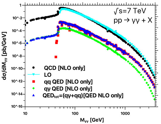
Figure 1. Invariant mass distribution of the two hardest photons. We present results for $\sqrt{s}=7$ TeV. The QCD corrections are computed using PDF4LHC, whilst the QED contributions were obtained with LUXqed.

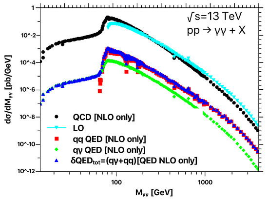
Figure 2. Invariant mass distribution of the two hardest photons. We present results for $\sqrt{s}=13$ TeV. The QCD corrections are computed using PDF4LHC, whilst the QED contributions were obtained with LUXqed.

The two different channels that are part of the total NLO QED correction, i.e., $q\overline{q}$ and $q\gamma$, are separately shown in the plots. The NLO QED corrections are moderate to tiny in the whole invariant-mass range. To quantitatively describe them, we define the ratio

$$K^{\mathrm{QED}}=\frac{{\delta }_{\mathrm{NLO}}^{\mathrm{QED}}}{{\delta }_{\mathrm{NLO}}^{\mathrm{QCD}}},$$

(24)

that reaches up to $4\%$ for $M_{\gamma \gamma }\gtrsim 2$ TeV. ${\sigma }_{\mathrm{NLO}}^{\mathrm{QED}}$ is dominated by the $q\overline{q}$ channel in almost the entire $M_{\gamma \gamma }$ range. The only exception is the low-mass region, which is forbidden at the LO due to kinematical constraints. The kinematics of the LO subprocess is determined by the two final-state photons. Since the only kinematical configuration allowed by the Born contribution is such that the two photons are back-to-back, $p_T^{\gamma \gamma }=0$ (i.e., $p_T^{\mathrm{harder}}=p_T^{\mathrm{softer}}$) and therefore, only the value of $p_T^{\mathrm{harder}}$ is effective as cut at LO,

$$M_{\gamma \gamma }\ge 2p_T^{\mathrm{harder}}.$$

(25)

Specifically, $M_{\gamma \gamma }\ge 50$ GeV for photon-pair production at $\sqrt{s}=7$ TeV (and its associated LHC cuts) and $M_{\gamma \gamma }\ge 80$ GeV for diphoton production at $\sqrt{s}=13$ TeV. Perturbative calculations in regions around unphysical fixed-order thresholds are known [67] to be generally affected by perturbative instabilities at higher orders. The invariant mass distribution is very steep in the kinematical region around the LO threshold and even the effect of little instabilities is amplified by the large slope of $d\sigma /d{M}_{\gamma \gamma }$. Therefore, in order to obtain reliable predictions around the LO threshold in $d\sigma /d{M}_{\gamma \gamma }$ it is enough to consider a bin size of roughly 2 GeV since we are dealing with integrable singularities [21,67].

The suppression of the $q\overline{q}$ channel in the low-mass region is an artifact of the ordering in the transverse momentum of the final state photons. This ordering procedure reproduces the selection algorithm implemented by the LHC. It is worth noticing that we can describe quantitatively the interplay among the kinematical cuts, the ordering and the position of the threshold in the $q\overline{q}$ channel. Let us consider a system with three massless on-shell particles in the center-of-mass frame. After ordering, we have

$$p_{T,1}\ge p_{T,2}\ge p_{T,3},\sum _{i=1}^3{\overrightarrow{p}}_{T,i}=0,$$

(26)

with ${\overrightarrow{p}}_i={\overrightarrow{p}}_{T,i}+{\overrightarrow{p}}_{L,i}$ and ${\overrightarrow{p}}_{T,i}·{\overrightarrow{p}}_{L,i}=0$. In fact, the transverse momentum conservation implies $p_{T,3}^2={|{\overrightarrow{p}}_{T,1}+{\overrightarrow{p}}_{T,2}|}^2$, and the ordering condition leads to

$$p_{T,2}^2\ge p_{T,3}^2=p_{T,1}^2+p_{T,2}^2+2p_{T,1}{p}_{T,2}cos{\theta }_{12}\leftrightarrow cos{\theta }_{12}\le -\frac{p_{T,1}}{2p_{T,2}},$$

(27)

where ${\theta }_{12}$ is the angular separation in the transverse plane. Since $p_{T,2}\le p_{T,1}$ by definition, we conclude that $2\pi /3\le {\theta }_{12}\le \pi$. So, we explicitly find a constraint in the angular separation of the transverse momenta of the hardest particles by imposing an ordering condition. Of course, such a restriction is not present when selecting randomly two photons and using their momenta to classify the event, as we did for the QCD corrections to $pp\to \gamma \gamma +X$. Moreover, from Equation (27) we can appraise that $p_{T,2}\le p_{T,1}\le 2p_{T,2}$, which constitutes another constraint.

On the other hand, it is crucial to notice that imposing both the transverse momenta ordering and the $p_T$ cuts detailed in Section 2, we end up with a cut in $M_{\gamma \gamma }$. To find the minimum allowed value for $M_{\gamma \gamma }$ distributions measured at ATLAS with $\sqrt{s}=7\mathrm{TeV}$, we choose $p_{T,1}=25\mathrm{GeV}$ and $p_{T,2}=22\mathrm{GeV}$. Then, inserting these values in Equation (27), we find

$${\theta }_{12}^{min}\approx 0.6924\pi ,$$

(28)

that increases the minimal angular separation between the transverse momenta of the hardest photons. Besides this, the invariant mass of the hardest subsystem is given by

$$M_{\gamma \gamma }=\sqrt{2p_1·p_2}=\sqrt{2E_1{E}_2(1-cos{\varphi }_{12})},$$

(29)

where ${\varphi }_{12}$ is the angle between ${\overrightarrow{p}}_1$ and ${\overrightarrow{p}}_2$. This angle is measured in the plane containing both three-vectors, which is not equivalent to the transverse plane to the colliding axis: thus, in general, ${\varphi }_{12}\ne {\theta }_{12}$. However, we impose ${\varphi }_{12}={\theta }_{12}$ in order to find the minimal invariant mass configuration. This choice is equivalent to settle the production of the triphoton system in the transverse plane, which leads to $E_1=p_{T,1}$, $E_2=p_{T,2}$ and

$$M_{\gamma \gamma }^{\min }=\sqrt{2p_{T,1}{p}_{T,2}(1-cos{\theta }_{12}^{min})}\approx 41.53\mathrm{GeV}.$$

(30)

Below these limit, the $q\overline{q}\to \gamma \gamma \gamma$ channel is not compatible with the experimental cuts. Analogously, when dealing with ATLAS measurements at $\sqrt{s}\ge 13\mathrm{TeV}$, we find

$${\theta }_{12}^{min}\approx 0.7323\pi ,M_{\gamma \gamma }^{\min }\approx 63.25\mathrm{GeV}.$$

(31)

These results explain the behavior of the distributions shown in Figure 1 and Figure 2, in particular, the steeply suppression of the cross-section in the region $M_{\gamma \gamma }\approx 41\mathrm{GeV}$ for $\sqrt{s}\ge 7\mathrm{TeV}$ and $M_{\gamma \gamma }\approx 63\mathrm{GeV}$ for $\sqrt{s}\ge 13\mathrm{TeV}$.

In Figure 3, we present the results for the transverse momentum distribution of the two hardest photons for $\sqrt{s}=13$ TeV. We compare the NLO QCD and NLO QED corrections, as well as the individual channels contributing to the last one. Notice that in the whole $p_T^{\gamma \gamma }$ range (with the exception of $p_T^{\gamma \gamma }=0$ GeV), these are effective LO contributions. As we appraised from Figure 1 and Figure 2, the $q\gamma$ channel for the invariant mass distribution was sub-dominant (and almost negligible) in all kinematical regions except the low-mass region.

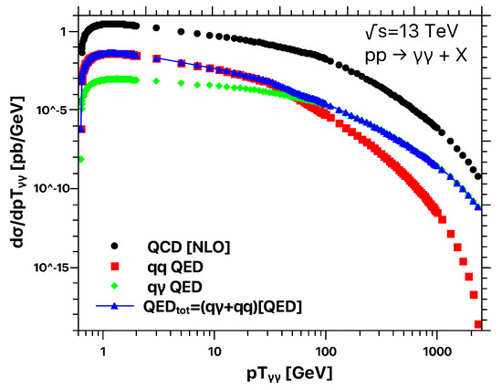
Figure 3. Transverse momentum distribution of the two hardest photons for $\sqrt{s}=13$ TeV. We present results for the NLO QCD prediction (black dots) and the NLO QED distribution (blue dashed triangles). In the case of the NLO QED prediction, we also present its two different channels: the $q\overline{q}$ channel (red squared dots) and the $q\gamma$ channel (green diamonds).

This can be regarded as a hint of what we are obtaining after the shoulder ($p_T^{\gamma \gamma }>70$ GeV) in the $p_T^{\gamma \gamma }$ distribution for the QED corrections: $q\gamma$ dominates the NLO QED cross section.

We present also two different ratios between the NLO QCD corrections and possible estimates of the higher-order QED corrections in Figure 4. Besides $K^{\mathrm{QED}/\mathrm{QCD}}$, we define

$$K^{\mathrm{QED}}\left({\mu }_R\right)=\frac{{\delta }_{\mathrm{NLO}}^{\mathrm{QED}}\left({\mu }_R\right)}{{\delta }_{\mathrm{NLO}}^{\mathrm{QCD}}},$$

(32)

where ${\delta }_{\mathrm{NLO}}^{\mathrm{NLO}\mathrm{QED}}\left({\mu }_R\right)$ denotes the NLO QED correction including running effects (as described in Section 2.1). Both $K^{\mathrm{QED}}\left({\mu }_R\right)$ and $K^{\mathrm{QED}}$ are similar for $0\le p_T^{\gamma \gamma }\le 1\mathrm{TeV}$. It is a well-known fact that QCD transverse momentum resummation is requested to recover the reliability of the calculation and improve the description of data in the low $p_T^{\gamma \gamma }$ region [20]. The same consideration applies here for the NLO QED corrections and the resummation QED program, which will be presented in a forthcoming paper.

Figure 4. The ratios between the NLO QCD corrections and the different estimates of the QED corrections, as a function of the diphoton transverse momentum $p_T^{\gamma \gamma }$. We consider the default choice with a frozen EM coupling (red dots) and an alternative one including running effects (green dots).

In order to explore additional measurements that could be more sensitive to QED corrections, we define a jet-veto algorithm to partially suppress the QCD components. In the first place, we consider only jets produced by QCD partons since we assume that photons can be unambiguously identified. Of course, from the experimental point of view, this is not completely true: highly energetic photons might decay into hadrons and they could be reconstructed as a jet. However, we claim that these effects are related to higher-order corrections beyond NLO QED, and that the jet identification is well-defined within the theoretical computation (at least at this perturbative order). So, after generating the event, we request the jet to be generated by a quark or gluon (but not by a photon) and to be observable within the detector. Then, we reject all the events with $p_T^{\mathrm{jet}}\ge 50\mathrm{GeV}$ and $\mid {\eta }_{\mathrm{jet}}\mid \le 2.37$. It is worth emphasizing that this definition is IR safe at this perturbative order, since all the IR-singular configurations automatically pass the cuts. (This jet-veto algorithm properly works for computing NLO corrections, since only one extra-parton is present in the final state. At NNLO and beyond, some subtleties could arise and the algorithm should be carefully redefined).

After this discussion, we consider the diphoton production for $\sqrt{s}=13$ TeV with an additional jet-veto in Figure 5. In the left panel, we show the effects on the different contributions of the total cross section. The NLO QCD correction is noticeably reduced beyond the veto threshold (i.e., $p_T^{\mathrm{jet}}=p_T^{\gamma \gamma }=50\mathrm{GeV}$), as well as the $q\gamma$ channel contribution to the NLO QED correction. We can appraise a discontinuity in the distribution at $p_T^{\gamma \gamma }=50\mathrm{GeV}$ because of the modification of the event selection criteria imposed by the jet-veto. Of course, this is something artificial and not related to any underlying physical phenomena. Furthermore, as expected, since the $\mathcal{O}\left(\alpha \right)$ corrections to the $q\overline{q}$ channel are associated to the process $q\overline{q}\to \gamma \gamma \gamma$, this process is not affected by the jet-veto and is not suppressed. In order to quantify these effects, we extend the definition of the ratios given in Equations (24) and (32) introducing

$$\begin{array}{ccc}\hfill K^{\mathrm{QED},JV}& =& \frac{\delta {\sigma }_{\mathrm{NLO}}^{\mathrm{QED},JV}}{\delta {\sigma }_{\mathrm{NLO}}^{\mathrm{QCD},JV}},\hfill \end{array}$$

(33)

$$\begin{array}{ccc}\hfill K^{\mathrm{QED},JV}\left({\mu }_R\right)& =& \frac{\delta {\sigma }_{\mathrm{NLO}}^{\mathrm{QED},JV}\left({\mu }_R\right)}{\delta {\sigma }_{\mathrm{NLO}}^{\mathrm{QCD},JV}},\hfill \end{array}$$

(34)

$$\begin{array}{ccc}\hfill K^{\mathrm{QED}\times \mathrm{QCD},JV}& =& \frac{\delta {\sigma }_{\mathrm{NLO}}^{\mathrm{QCD}\times \mathrm{QED},JV}}{\delta {\sigma }_{\mathrm{NLO}}^{\mathrm{QCD},JV}},\hfill \end{array}$$

(35)

where the additional superscript denotes that we are taking into account the jet-veto. The results are shown in the right panel of Figure 5. While the low $p_T^{\gamma \gamma }$ region is similar to the one without imposing the jet-veto (see Figure 3), at large values of transverse momentum (in particular for $p_T^{\gamma \gamma }\gtrsim 600$ GeV) the $q\overline{q}$ channel dominates the total cross section, and the ratios reach $\mathcal{O}(10\%)$.

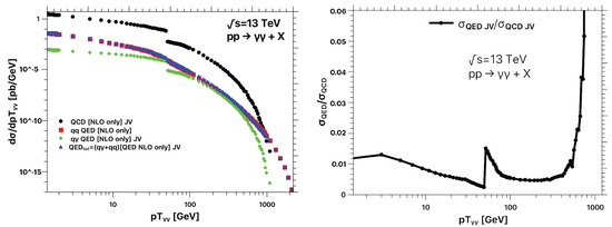
Figure 5. (Left) Transverse momentum distribution of the two hardest photons for $\sqrt{s}=13$ TeV with a jet-veto applied. (Right) The ratios between the different estimates of the higher-order QED and the NLO QCD corrections, as a function of $p_T^{\gamma \gamma }$. It is possible to clearly identify the jet-veto threshold at $p_T^{\gamma \gamma }=50\mathrm{GeV}$ due to the discontinuity in the ratios.

As next, we present the transverse momentum distributions of the hardest ($p_T^{\gamma ,H}$) and second hardest ($p_T^{\gamma ,S}$) photons in Figure 6. The $p_T^{\gamma ,H}$ distribution is strongly affected neither by the NLO QED corrections nor by the estimated mixed QCD-QED contributions. Even if a jet-veto is applied, the NLO QED corrections for this observable are still negligible, because the LO and NLO QCD terms are much more relevant.

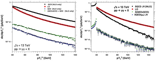
Figure 6. Transverse momentum distribution of the hardest (left) and second hardest (right) photons at $\sqrt{s}=13$ TeV. We compare the Born contribution with the NLO QCD correction and the NLO QED contributions with $\alpha =1/137$ and with $\alpha \left({\mu }_R\right)$.

On the contrary, we notice strong effects due to the jet-veto in the $p_T^{\gamma ,S}$ distribution: an important suppression of the total NLO QCD corrections and the $q\gamma$ channel are shown in Figure 6 (right panel). Since the NLO QED cross section is dominated by the $q\overline{q}$ channel, which is not affected by the jet-veto, an enhancement of the QED-to-QCD ratios takes place. The estimate of the mixed QCD-QED corrections is similar to the one obtained when considering the running of $\alpha$. The exception to this behavior is found in the low transverse momentum region (i.e., $p_T^{\gamma ,S}\leqq 40$ GeV), since it is populated with real-radiation events appearing for the first time in the NLO contributions. It is worth emphasizing that the higher-order QED terms introduce corrections of $\mathcal{O}(10\%)$ of the total NLO QCD contributions for $p_T^{\gamma ,S}\backsim 140$ GeV.

In Figure 7, we present our results for the transverse momentum distribution of the two hardest photons but using the distributions of the set NNPDF3.0QED. We compare the NLO QCD cross section with the NLO QED contribution, considering also in particular its two channels: $q\gamma$ and $q\overline{q}$. The main differences with the results using the LUXqed PDFs, detailed in Figure 3, are due to the $q\gamma$ channel. Even if there is a disagreement among them, due to an enhancement of the $q\gamma$ channel in the middle and high-energy region, we should consider the predictions obtained with NNPDF3.0QED as a qualitative estimate in that region.

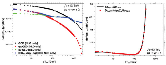
Figure 7. Transverse momentum distribution of the two hardest photons for $\sqrt{s}=13$ TeV using NNPDF3.0QED PDFs. In the right panel we show the ratios between the NLO QCD corrections and the different estimates of the QED corrections, as a function of the diphoton transverse momentum $p_T^{\gamma \gamma }$. We consider the default choice with a frozen EM coupling (black line) and an alternative one including running effects (red dots). We appraise that the NLO QED cross-sections obtained with NNPDF3.0QED are much larger than those for LUXqed in the high-energy region due to the $q\gamma$ channel.

We would like to emphasize here that the purpose of the previous comparison is to highlight that different methodologies on the extraction of PDFs could have a noticeable impact of the phenomenological analysis. In particular, a purely data-driven extraction of PDFs suffers from the lack of good-quality data-points in some regions of the parameter space, which directly impact in the error propagation. The methodology applied for extracting NNPDF3.0QED is more sensible to the lack of experimental points for very high energies, which leads to huge errors in the $x\approx 1$ region. The approach followed by LUXqed uses all-order theoretical predictions to constrain the photon PDF with data-points in the low-energy region, thus reducing the fitting errors. It is worth noticing that the updated versions of NNPDF combine the methodology developed by LUXqed in order to improve the predictions for the photon PDF [68,69,70], leading to an impressive increase on the precision achieved.

Finally, we comment about two other aspects of this computation. In the first place, we explore the effects due to the merging algorithm for photons, as described in Section 2.1. For $0.05\le \Delta R_{\gamma \gamma }^{\min }\le 0.1$, both the $E_0$ and E-schemes present significant deviations neither between these nor compared with the distributions obtained without any clustering algorithm. The precedent consideration is valid for the total cross section, as well as for all the differential distributions presented in this work. Thus, we conclude that the implementation of a clustering algorithms with the current experimental conditions has a negligible impact in the measurements, which is compatible with the experimental and theoretical uncertainties.

4. Conclusions

A discussion about the computation of NLO QED corrections to diphoton production was presented, putting special emphasis in the phenomenological aspects for hadron colliders. Besides the size of these contributions and the (partial) estimate of the mixed QCD-QED terms, we emphasize that keeping under control all the possible uncertainties in this process is crucial since it is the main background for many new physics searches. Taking under control the QED corrections at the LHC allows to potentially decide about the origin of future discrepancies between data and theory. Moreover, the importance of high-precision predictions becomes completely indispensable when considering the next generation of high-energy and high-luminosity experiments [6,7,8,9,10,11,12,13].

In this article, NLO QED corrections were obtained through the application of the QED version of the $q_T$-subtraction method, after a proper Abelianization of the NLO QCD implementation available in the program 2$\gamma$NNLO. It is important to notice that we carefully studied the cancellation of IR singularities in the $q_T\to 0$ limit, in order to guarantee the theoretical consistency of the approach.

In general, we found small corrections for the $M_{\gamma \gamma }$ distribution, whilst the ratio $K^{\mathrm{QED}}$ reaches $\mathcal{O}(10\%)$ for the $p_T^{\gamma \gamma }$ spectrum. This is because only the real-emission terms contribute to the cross-section for $p_T^{\gamma \gamma }>0$: a simple power counting shows that the QED-to-QCD ratio behaves like $\alpha /{\alpha }_{\mathrm{S}}\approx 10\%$. Besides that, we studied the effects due to the treatment of the EM running coupling, which could also introduce percent-level effects in all the distributions considered.

An interesting observation is that the $q\gamma$ channel is not always negligible, specially in some kinematical regions for distributions involving the transverse momentum. For instance, it dominates the NLO QED corrections to the $p_T^{\gamma \gamma }$ distribution for moderate values of transverse momentum, i.e., $p_T^{\gamma \gamma }\gtrsim 80$ GeV, as we showed in Figure 3. From this results, we conclude that it is always recommended to include the photon-initiated processes when computing differential distributions.

Besides that, using the approach described in Ref. [66], we provided an estimate of the mixed QCD-QED corrections. Other interesting effects were found when considering the dependence on $p_T^{\gamma \gamma ,S}$ (the transverse momentum of the second hardest photon), exhibiting $\mathcal{O}(10\%)$ corrections relative to the NLO QCD contributions. These effects are enhanced when including a jet-veto to suppress the QCD component, although the $M_{\gamma \gamma }$ distribution was slightly modified.

Finally, we would like to highlight that QED corrections cannot be neglected in the context of precision high-energy physics. Moreover, such computations must be done within a fully consistent framework, which carefully includes all the ingredients without introducing additional sources of uncertainties.

References

- De Florian, D.; Sborlini, G.F.R. Hadron plus photon production in polarized hadronic collisions at next-to-leading order accuracy. Phys. Rev. D 2011, 83, 074022. [Google Scholar] [CrossRef]
- Rentería-Estrada, D.F.; Hernández-Pinto, R.J.; Sborlini, G.F.R. Analysis of the internal structure of hadrons using direct photon production. arXiv 2021, arXiv:2104.14663. [Google Scholar]
- Aad, G.; Abajyan, T.; Abbott, B.; Abdallah, J.; Khalek, S.A.; Abdelalim, A.A.; Aben, R.; Abi, B.; Abolins, M.; AbouZeid, O.S.; et al. Observation of a new particle in the search for the Standard Model Higgs boson with the ATLAS detector at the LHC. Phys. Lett. B 2012, 716, 1–29. [Google Scholar] [CrossRef]
- Chatrchyan, S.; Khachatryan, V.; Sirunyan, A.M.; Tumasyan, A.; Adam, W.; Aguilo, E.; Bergauer, T.; Dragicevic, M.; Erö, J.; Fabjan, C.; et al. Observation of a New Boson at a Mass of 125 GeV with the CMS Experiment at the LHC. Phys. Lett. B 2012, 716, 30–61. [Google Scholar] [CrossRef]
- Mangano, M. LHC at 10: The physics legacy. CERN Cour. 2020, 60, 40. [Google Scholar]
- FCC Collaboration. FCC Physics Opportunities: Future Circular Collider Conceptual Design Report Volume 1. Eur. Phys. J. C 2019, 79, 474. [Google Scholar] [CrossRef]
- FCC Collaboration. FCC-ee: The Lepton Collider: Future Circular Collider Conceptual Design Report Volume 2. Eur. Phys. J. ST 2019, 228, 261–623. [Google Scholar] [CrossRef]
- FCC Collaboration. FCC-hh: The Hadron Collider: Future Circular Collider Conceptual Design Report Volume 3. Eur. Phys. J. ST 2019, 228, 755–1107. [Google Scholar] [CrossRef]
- FCC Collaboration. HE-LHC: The High-Energy Large Hadron Collider: Future Circular Collider Conceptual Design Report Volume 4. Eur. Phys. J. ST 2019, 228, 1109–1382. [Google Scholar] [CrossRef]
- Blondel, A.; Gluza, J.; Jadach, S.; Janot, P.; Riemann, T. (Eds.) Theory for the FCC-ee: Report on the 11th FCC-eeWorkshop theory and experiments. In CERN Yellow Reports: Monographs; CERN: Geneva, Switzerland, 2019. [Google Scholar] [CrossRef]
- Bambade, P.; Barklow, T.; Behnke, T.; Berggren, M.; Brau, J.; Burrows, P.; Denisov, D.; Faus-Golfe, A.; Foster, B.; Fujii, K.; et al. The International Linear Collider: A Global Project. arXiv 2019, arXiv:1903.01629. [Google Scholar]
- Roloff, P.; Franceschini, R.; Schnoor, U.; Wulzer, A. The Compact Linear e+e− Collider (CLIC): Physics Potential. arXiv 2018, arXiv:1812.07986. [Google Scholar]
- CEPC Study Group. CEPC Conceptual Design Report: Volume 2 - Physics & Detector. arXiv 2018, arXiv:1811.10545. [Google Scholar]
- Binoth, T.; Guillet, J.P.; Pilon, E.; Werlen, M. A Full next-to-leading order study of direct photon pair production in hadronic collisions. Eur. Phys. J. C 2000, 16, 311–330. [Google Scholar] [CrossRef]
- Bern, Z.; Dixon, L.J.; Schmidt, C. Isolating a light Higgs boson from the diphoton background at the CERN LHC. Phys. Rev. D 2002, 66, 074018. [Google Scholar] [CrossRef]
- Campbell, J.M.; Ellis, R.K.; Williams, C. Vector boson pair production at the LHC. J. High Energy Phys. 2011, 7, 18. [Google Scholar] [CrossRef]
- Balazs, C.; Berger, E.L.; Nadolsky, P.M.; Yuan, C.P. Calculation of prompt diphoton production cross-sections at Tevatron and LHC energies. Phys. Rev. D 2007, 76, 013009. [Google Scholar] [CrossRef]
- Catani, S.; Cieri, L.; de Florian, D.; Ferrera, G.; Grazzini, M. Diphoton production at hadron colliders: A fully-differential QCD calculation at NNLO. Phys. Rev. Lett. 2012, 108, 072001. [Google Scholar] [CrossRef]
- Campbell, J.M.; Ellis, R.K.; Li, Y.; Williams, C. Predictions for diphoton production at the LHC through NNLO in QCD. J. High Energy Phys. 2016, 7, 148. [Google Scholar] [CrossRef]
- Cieri, L.; Coradeschi, F.; de Florian, D. Diphoton production at hadron colliders: Transverse-momentum resummation at next-to-next-to-leading logarithmic accuracy. J. High Energy Phys. 2015, 6, 185. [Google Scholar] [CrossRef]
- Catani, S.; Cieri, L.; de Florian, D.; Ferrera, G.; Grazzini, M. Diphoton production at the LHC: A QCD study up to NNLO. J. High Energy Phys. 2018, 4, 142. [Google Scholar] [CrossRef]
- Butterworth, J.; Dissertori, G.; Dittmaier, S.; de Florian, D.; Glover, N.; Hamilton, K.; Huston, J.; Kado, M.; Korytov, A.; Krauss, F.; et al. Les Houches 2013: Physics at TeV Colliders: Standard ModelWorking Group Report. arXiv 2014, arXiv:1405.1067. [Google Scholar]
- Badger, S.; Bendavid, J.; Ciulli, V.; Denner, A.; Frederix, R.; Grazzini, M.; Huston, J.; Schönherr, M.; Tackmann, K.; Thaler, J.; et al. Les Houches 2015: Physics at TeV Colliders Standard Model Working Group Report. arXiv 2016, arXiv:1605.04692. [Google Scholar]
- Cieri, L.J. Particle Production at Hadron Colliders. Ph.D. Thesis, Buenos Aires University, Buenos Aires, Argentina, 2012. [Google Scholar]
- Cieri, L.J. Diphoton spectrum in the mass range 120-140 GeV at the LHC. arXiv 2012, arXiv:1207.3252. [Google Scholar]
- Catani, S.; Fontannaz, M.; Guillet, J.P.; Pilon, E. Cross-section of isolated prompt photons in hadron hadron collisions. J. High Energy Phys. 2002, 5, 28. [Google Scholar] [CrossRef]
- Catani, S.; Fontannaz, M.; Guillet, J.P.; Pilon, E. Isolating Prompt Photons with Narrow Cones. J. High Energy Phys. 2013, 9, 7. [Google Scholar] [CrossRef]
- Binoth, T.; Guillet, J.P.; Pilon, E.; Werlen, M. Beyond leading order effects in photon pair production at the Tevatron. Phys. Rev. D 2001, 63, 114016. [Google Scholar] [CrossRef]
- Amoroso, S.; Azzurri, P.; Bendavid, J.; Bothmann, E.; Britzger, D.; Brooks, H.; Buckley, A.; Calvetti, M.; Chen, X.; Chiesa, M.; et al. Les Houches 2019: Physics at TeV Colliders: Standard Model Working Group Report. arXiv 2020, arXiv:2003.01700. [Google Scholar]
- Gehrmann, T.; Glover, N.; Huss, A.; Whitehead, J. Scale and isolation sensitivity of diphoton distributions at the LHC. J. High Energy Phys. 2021, 1, 108. [Google Scholar] [CrossRef]
- Kawabata, S.; Yokoya, H. Top-quark mass from the diphoton mass spectrum. Eur. Phys. J. C 2017, 77, 323. [Google Scholar] [CrossRef]
- Dugad, S.R.; Jain, P.; Mitra, S.; Sanyal, P.; Verma, R.K. The top threshold effect in the γγ production at the LHC. Eur. Phys. J. C 2018, 78, 715. [Google Scholar] [CrossRef]
- Frixione, S. Isolated photons in perturbative QCD. Phys. Lett. B 1998, 429, 369–374. [Google Scholar] [CrossRef]
- Cieri, L. Diphoton isolation studies. Nucl. Part. Phys. Proc. 2016, 273, 2033–2039. [Google Scholar] [CrossRef]
- Denner, A.; Dittmaier, S.; Kasprzik, T.; Muck, A. Electroweak corrections to W + jet hadroproduction including leptonic W-boson decays. J. High Energy Phys. 2009, 8, 75. [Google Scholar] [CrossRef]
- Denner, A.; Dittmaier, S.; Hecht, M.; Pasold, C. NLO QCD and electroweak corrections to W+γ production with leptonic W-boson decays. J. High Energy Phys. 2015, 4, 018. [Google Scholar] [CrossRef]
- Denner, A.; Dittmaier, S.; Hecht, M.; Pasold, C. NLO QCD and electroweak corrections to Z+γ production with leptonic Z-boson decays. J. High Energy Phys. 2016, 2, 057. [Google Scholar] [CrossRef]
- Bonciani, R.; Buccioni, F.; Mondini, R.; Vicini, A. Double-real corrections at (ααs) to single gauge boson production. Eur. Phys. J. C 2017, 77, 187. [Google Scholar] [CrossRef]
- Sborlini, G.F.R. Including higher-order mixed QCD-QED effects in hadronic calculations. arXiv 2018, arXiv:1805.06192. [Google Scholar]
- Cieri, L.; Ferrera, G.; Sborlini, G.F.R. Combining QED and QCD transverse-momentum resummation for Z boson production at hadron colliders. J. High Energy Phys. 2018, 8, 165. [Google Scholar] [CrossRef]
- Bierweiler, A.; Kasprzik, T.; Kühn, J.H. Vector-boson pair production at the LHC to (α3) accuracy. J. High Energy Phys. 2013, 12, 71. [Google Scholar] [CrossRef]
- Chiesa, M.; Greiner, N.; Schönherr, M.; Tramontano, F. Electroweak corrections to diphoton plus jets. J. High Energy Phys. 2017, 10, 181. [Google Scholar] [CrossRef]
- Greiner, N.; Schönherr, M. NLO QCD+EW corrections to diphoton production in association with a vector boson. J. High Energy Phys. 2018, 1, 79. [Google Scholar] [CrossRef]
- Sborlini, G.F.R. Higher-order QED effects in hadronic processes. arXiv 2017, arXiv:1709.09596. [Google Scholar]
- De Florian, D.; Sborlini, G.F.R.; Rodrigo, G. QED corrections to the Altarelli–Parisi splitting functions. Eur. Phys. J. C 2016, 76, 282. [Google Scholar] [CrossRef]
- De Florian, D.; Sborlini, G.F.R.; Rodrigo, G. Two-loop QED corrections to the Altarelli-Parisi splitting functions. J. High Energy Phys. 2016, 10, 56. [Google Scholar] [CrossRef]
- Sborlini, G.F.R.; de Florian, D.; Rodrigo, G. Mixed QCD-QED corrections to DGLAP equations. arXiv 2016, arXiv:1611.04785. [Google Scholar]
- Contino, R.; Kramer, T.; Son, M.; Sundrum, R. Warped/composite phenomenology simplified. J. High Energy Phys. 2007, 5, 74. [Google Scholar] [CrossRef]
- Catani, S.; Grazzini, M. An NNLO subtraction formalism in hadron collisions and its application to Higgs boson production at the LHC. Phys. Rev. Lett. 2007, 98, 222002. [Google Scholar] [CrossRef]
- Catani, S.; Cieri, L.; de Florian, D.; Ferrera, G.; Grazzini, M. Universality of transverse-momentum resummation and hard factors at the NNLO. Nucl. Phys. B 2014, 881, 414–443. [Google Scholar] [CrossRef]
- Cieri, L.; de Florian, D.; Der, M.; Mazzitelli, J. Mixed QCD⊗QED corrections to exclusive Drell Yan production using the qT-subtraction method. J. High Energy Phys. 2020, 9, 155. [Google Scholar] [CrossRef]
- Aad, G.; Abajyan, T.; Abbott, B.; Abdallah, J.; Khalek, S.A.; Abdelalim, A.A.; Aben, R.; Abi, B.; Abolins, M.; AbouZeid, O.S.; et al. Measurement of isolated-photon pair production in pp collisions at = 7 TeV with the ATLAS detector. J. High Energy Phys. 2013, 1, 086. [Google Scholar] [CrossRef]
- Çakır, O. Measurements of integrated and differential cross sections for isolated photon pair production in pp collisions at = 8 TeV with the ATLAS detector. Phys. Rev. D 2017, 95, 112005. [Google Scholar]
- Aaboud, M.; Aad, G.; Abbott, B.; Abdallah, J.; Abeloos, B.; Aben, R.; AbouZeid, O.S.; Abraham, N.L.; Abramowicz, H.; Abreu, H.; et al. Measurement of the photon identification efficiencies with the ATLAS detector using LHC Run-1 data. Eur. Phys. J. C 2016, 76, 666. [Google Scholar] [CrossRef]
- Bartel, W.; Becker, L.; Felst, R.; Haidt, D.; Knies, G.; Krehbiel, H.; Laurikainen, P.; Magnussen, N.; Meinke, R.; Naroska, B.; et al. Experimental Studies on Multi-Jet Production in e+e− Annihilation at PETRA Energies. Z. FüR Phys. Part. Fields 1986, 33, 23–31. [Google Scholar]
- Catani, S.; Dokshitzer, Y.L.; Olsson, M.; Turnock, G.; Webber, B.R. New clustering algorithm for multi-jet cross-sections in e+e− annihilation. Phys. Lett. B 1991, 269, 432–438. [Google Scholar] [CrossRef]
- Harland-Lang, L.A.; Khoze, V.A.; Ryskin, M.G. Sudakov effects in photon-initiated processes. Phys. Lett. B 2016, 761, 20–24. [Google Scholar] [CrossRef]
- Jegerlehner, F. Hadronic Contributions to Electroweak Parameter Shifts: A Detailed Analysis. Z. Phys. C 1986, 32, 195. [Google Scholar] [CrossRef]
- Burkhardt, H.; Jegerlehner, F.; Penso, G.; Verzegnassi, C. Uncertainties in the Hadronic Contribution to the QED Vacuum Polarization. Z. Phys. C 1989, 43, 497–501. [Google Scholar] [CrossRef]
- Eidelman, S.; Jegerlehner, F. Hadronic contributions to g-2 of the leptons and to the effective fine structure constant alpha (M(z)**2). Z. Phys. C 1995, 67, 585–602. [Google Scholar] [CrossRef]
- Manohar, A.; Nason, P.; Salam, G.P.; Zanderighi, G. How bright is the proton? A precise determination of the photon parton distribution function. Phys. Rev. Lett. 2016, 117, 242002. [Google Scholar] [CrossRef]
- Manohar, A.V.; Nason, P.; Salam, G.P.; Zanderighi, G. The Photon Content of the Proton. J. High Energy Phys. 2017, 12, 046. [Google Scholar] [CrossRef]
- Butterworth, J.; Carrazza, S.; Cooper-Sarkar, A.; De Roeck, A.; Feltesse, J.; Forte, S.; Gao, J.; Glazov, S.; Huston, J.; Kassabov, Z.; et al. PDF4LHC recommendations for LHC Run II. J. Phys. G 2016, 43, 023001. [Google Scholar] [CrossRef]
- Ball, R.D.; Bertone, V.; Carrazza, S.; Deans, C.S.; Del Debbio, L.; Forte, S.; Guffanti, A.; Hartland, N.P.; Latorre, J.I.; Rojo, J.; et al. Parton distributions with LHC data. Nucl. Phys. B 2013, 867, 244–289. [Google Scholar] [CrossRef]
- Ball, R.D.; Bertone, V.; Carrazza, S.; Deans, C.S.; Del Debbio, L.; Forte, S.; Guffanti, A.; Hartland, N.P.; Latorre, J.I.; Rojo, J.; et al. Parton distributions for the LHC Run II. J. High Energy Phys. 2015, 5, 40. [Google Scholar] [CrossRef]
- Kallweit, S.; Lindert, J.M.; Pozzorini, S.; Schönherr, M. NLO QCD+EW predictions for 2ℓ2ν diboson signatures at the LHC. J. High Energy Phys. 2017, 11, 120. [Google Scholar] [CrossRef]
- Catani, S.; Webber, B.R. Infrared safe but infinite: Soft gluon divergences inside the physical region. J. High Energy Phys. 1997, 10, 5. [Google Scholar] [CrossRef][Green Version]
- Bertone, V.; Carrazza, S.; Hartland, N.P.; Rojo, J. Illuminating the photon content of the proton within a global PDF analysis. SciPost Phys. 2018, 5, 8. [Google Scholar] [CrossRef]
- Campbell, J.M.; Rojo, J.; Slade, E.; Williams, C. Direct photon production and PDF fits reloaded. Eur. Phys. J. C 2018, 78, 470. [Google Scholar] [CrossRef] [PubMed]
- Khalek, R.A.; Ball, R.D.; Carrazza, S.; Forte, S.; Giani, T.; Kassabov, Z.; Nocera, E.R.; Pearson, R.L.; Rojo, J.; Rottoli, L.; et al. A first determination of parton distributions with theoretical uncertainties. Eur. Phys. J. 2019, 79, 838. [Google Scholar] [CrossRef]
Publisher’s Note: MDPI stays neutral with regard to jurisdictional claims in published maps and institutional affiliations. |
© 2021 by the authors. Licensee MDPI, Basel, Switzerland. This article is an open access article distributed under the terms and conditions of the Creative Commons Attribution (CC BY) license (https://creativecommons.org/licenses/by/4.0/).