Abstract
In this paper, we develop two algorithms to solve a nonlinear system of symmetric equations. The first is an algorithm based on modifying two Broyden–Fletcher–Goldfarb–Shanno (BFGS) methods. One of its advantages is that it is more suitable to effectively solve a small-scale system of nonlinear symmetric equations. In contrast, the second algorithm chooses new search directions by incorporating an approximation method of computing the gradients and their difference into the determination of search directions in the first algorithm. In essence, the second one can be viewed as an extension of the conjugate gradient method recently proposed by Lv et al. for solving unconstrained optimization problems. It was proved that these search directions are sufficiently descending for the approximate residual square of the equations, independent of the used line search rules. Global convergence of the two algorithms is established under mild assumptions. To test the algorithms, they are used to solve a number of benchmark test problems. Numerical results indicate that the developed algorithms in this paper outperform the other similar algorithms available in the literature.
Keywords:
nonlinear system of equations; computational method; algorithms; conjugate gradient method; global convergence MSC:
90c25; 90C30
1. Introduction
In this paper, we study solution methods of the following nonlinear system of symmetric equations:
where is a continuously differentiable function, and its Jacobian is symmetric, i.e., . Such a problem is closely related with many scientific problems, such as unconstrained optimization problems, equality constrained mathematical programming problems, discretized two-point boundary value problems, and discretized elliptic boundary value problems (see Chapter 1 in [1]). For example, when F is the gradient mapping of an objective function , (1) is just the first order necessary condition for a local minimizer of the following problem:
For the equality constrained mathematical programming problems:
where is a vector-valued function. The Karush–Kuhn–Tucker (KKT) conditions (see Chapter 8 in [2]) for Problem (3) is also the system (1) with , and:
Among various methods for solving (1), the Newton method needs to compute the Jacobian matrix , and requires that is nonsingular at each iterative point. Due to this stringent condition, the Newton method is not applicable in a general case.
Li and Fukushima [3] proposed a Gauss–Newton method to solve the symmetric system of equations, which can ensure that an approximate residual of is descent. Gu et al. [4] modified the method in [3] such that the residual is descent. As a generalization of the method in [5] for solving smooth unconstrained optimization, Zhou [6] presented an inexact modified BFGS method to solve the symmetric system of equations by approximately computing the gradient of the residual square. In [7], Wang and Zhu proposed an inexact-Newton via GMRES (generalized minimal residual) subspace method without line search technique for solving symmetric nonlinear equations. The iterative direction was obtained by solving the Newton equation of the system of nonlinear equations with the GMRES algorithm. Yuan and Yao [8] also proposed a BFGS method for solving symmetric nonlinear equations and the method possesses a good property that the generated sequence of the quasi-Newton matrix is positive definite. However, since the search direction is generated by solving a system of linear equations in these methods, all of them are not applicable to solving large-scale problems.
For large-scale symmetric nonlinear equations, Li and Wang [9] proposed a modified Fletcher–Reeves derivative-free method, as an extension of the conjugate gradient method [10]. Similarly, as an extension of descent conjugate gradient methods in [11] for unconstrained optimization, Xiao et al. [12] presented a family of derivative-free methods for symmetric equations, and established the global convergence under some appropriate conditions, and showed their effectiveness by numerical experiments. Zhou and Shen [13] presented an efficient iterative method for solving large-scale symmetric equations, as an extension of the three-term PRP conjugate gradient method in [14] for solving unconstrained optimization problems. Liu and Feng [15] proposed a norm descent derivative-free algorithm for solving large-scale nonlinear symmetric equations, as an extension of the three-term conjugate gradient method in [16] for solving unconstrained optimization problems. More details can be seen in [17,18,19,20].
Our motivation in this paper is to develop two algorithms to solve Problem (1). Firstly, based on the single-parameter scaling memoryless BFGS method proposed by Lv et al. [21] and the modification of the BFGS method in [22], we intended to develop an efficient algorithm (MSBFGS) which would incorporate the approximation method of computing the gradients in [3] and their difference in [6] such that it can solve the system of nonlinear Equations (1) more efficiently. Secondly, since MSBFGS is involved with computation and the storage of matrices, it is not applicable to solve a large-scale system of nonlinear equations. Therefore, by giving an inverse formula of the update matrix in MSBFGS, we are going to develop another method (MSBFGS2) such that it can solve large-scale systems of nonlinear Equations (1). Additionally, in addition to the establishment of the two algorithms’ convergence, we shall also demonstrate their powerful numerical performance as they are applied to solve benchmark test problems in the literature.
The rest of this paper is organized as follows. In Section 2, we first state the idea to propose two methods for solving the nonlinear symmetric equations. Then, two new algorithms are developed. Global convergence of algorithms is established in Section 3. Section 4 is devoted to numerical tests. Some conclusions are drawn in Section 5.
Some words about our notation: throughout the paper, the space is equipped with the Euclidean norm , the transpose of any matrix is denoted by , and the and are abbreviated as and , respectively.
2. Development of Algorithm
In this section, we first simply recall a single-parameter scaling BFGS method [21] for solving the following unconstrained optimization problem:
where is continuously differentiable such that its gradient is available. This method generates a sequence satisfying:
where , is the initial point, is called a step length obtained by some line search rule, and is a search direction defined as
where .
By minimizing the measure function introduced by Byrd and Nocedal [23]:
Lv et al. [21] obtained that:
In 2006, ref. [22] proposed a modification of the BFGS algorithm for unconstrained nonconvex optimization. The matrix in [22] was updated by the formula:
where is the sum of and , and .
Due to their impressive numerical efficiency, we now attempt to modify the aforementioned methods to solve the symmetric system of nonlinear Equation (1).
Then, for this objective function, any global minimizer of Problem (5) at which f vanishes is a solution of Problem (1). If an algorithm stops at a global minimizer , i.e., , then the algorithm finds a solution of (1).
By a symmetry of J, it holds that
In [3], Li and Fukushima suggested that is approximately computed by
where , and it can be proved that:
In other words, when is sufficiently small, it is true that the vector defined by (13) is a nice approximation to .
In the actual calculation, [3] computed by
where is the step size at the last iterate point . In general, the convergence of algorithms can ensure that .
Based on the work done by Li and Fukushima [3], Zhou [6] proposed a modified BFGS method to solve (1). The modified BFGS update formula is given by
where:
and:
Based on the ideas of [6,21,22], we now attempt to propose a modified single-parameter scaling BFGS method to solve (1). The modified BFGS update formula is given by
where and:
Moreover, we obtain an approximate quasi-Newton direction:
where is an approximate gradient defined by (15).
Remark 1.
in (20) is slightly different from that in (17) where . Since in (21) can minimize (8) where is defined by (19), its condition number which is the quotient of the maximum eigenvalue and the minimum eigenvalue of is also minimized. Clearly, a smaller condition number of search direction matrices can theoretically ensure the stability of algorithms [21]. Numerical experiments will also show that in (19) with being defined by (21) is more efficient and robust than that in (16).
Since nonmonotone line search rules can play a critical role in solving a complicated nonconvex optimization problem, we use the nonmonotone line search in [3,6] to determine a step-size along the direction . Specifically, let and be five given constants, and let be a given positive sequence such that:
We search for a step size satisfying:
With the above preparation, we are in a position to develop an algorithm to solve Problem (1). We now present its computer procedure as follows.
Remark 2.
Since Algorithm 1 cannot efficiently solve large-scale nonlinear symmetric equations, based on the work done by [3], we will develop another algorithm that is not involved with matrix operation and inverse operation. When we set , the inverse matrix of in (19) can be written as
where is the same as (21), and:
In fact, and are completely the same as those in [3,15].
Moreover, in order to guarantee that our proposed method generates descent directions and to further increase its computational efficiency and robustness, we can compute the direction by
where is defined in (15) and:
Remark 4.
Since the search direction of Algorithm 1 at each iteration is an approximate quasi-Newton direction, which is involved with the solution of a linear system of equations, Algorithm 1 can only efficiently solve small–medium-scale Problem (1). Instead, the needed search directions in Algorithm 2 is only associated with evaluating the function F without requirement of computing or storing its Jacobian matrix. Thus, compared with Algorithm 1, Algorithm 2 is more applicable to solving large-scale systems of nonlinear equations. In addition, two different approximation methods are used to compute the difference of gradients (see (18) and (28)).
| Algorithm 1 (Modified Single-Parameter Scaling BFGS Algorithm (MSBFGS)) |
| Step 0. Choose three constants . Take a sequence satisfying (23). Arbitrarily choose an initial iterate point , a symmetric and positive definite matrix . Set . |
| Step 1. If is satisfied, then the algorithm stops. |
| Step 2. Compute by (22) and (19). |
| Step 3. Determine a step length satisfying (24). |
| Step 4. Set . |
| Step 5. Set , return to Step 1. |
| Algorithm 2 (Modified Single-Parameter Scaling BFGS Algorithm 2(MSBFGS2)) |
| Step 0. Choose three constants . Take a sequence satisfying (23). Arbitrarily choose an initial iterate point . Set . |
| Step 1. If is satisfied, then the algorithm stops. |
| Step 2. Compute by (29). |
| Step 3. Determine a step length satisfying: |
| Step 4. Set . |
| Step 5. Set , return to Step 1. |
Remark 5.
By combining the advantages of the three-term conjugate gradient method in [21] and those of the approximation methods for computing the difference of gradients, it is believable that the numerical performance of Algorithm 2 is better than the algorithm in [21]. In the two subsequent sections, apart from establishing the convergence theory of Algorithm 2, we will also test its efficiency in solving large-scale problems.
3. Convergence of Algorithm
In this section, we establish the global convergence of Algorithms 1 and 2. For this purpose, we first define the level set:
Clearly, it follows from Step 3 of Algorithm 1 that:
Thus, any sequence generated by Algorithm 1 belongs to , i.e., for all k. In other words, there exists a constant , such that:
Moreover, since satisfies (23), from Lemma 3.3 in [24], we know that the sequence generated by Algorithm 1 converges.
Likewise, from the line search rule of Algorithm 2, we know that the sequence of iterate points generated by Algorithm 2 also belongs to and generated by Algorithm 2 also satisfies (34).
As done in the existing results [13,15,25], we also suppose that F in (1) satisfies the following conditions:
Assumption 1.
The solution set of the problem (1) is nonempty.
Assumption 2.
The level set Ω is bounded.
Assumption 3.
F is a continuous differentiable on an open and convex set containing the level set Ω, and its Jacobian matrix is symmetric and bounded on V, i.e., there exists a positive constant M such that:
Assumption 4.
is uniformly nonsingular on V, i.e., there exists a positive constant m such that:
Clearly, Assumptions 2–4 imply that there exist positive constants such that the following statements are true:
(1) For any , ,
(2) For any ,
where .
(3) For any sequence ,
where .
Under Assumptions 2–4, we can prove that Algorithm 1 has the following nice properties.
Lemma 1.
Let be generated by the BFGS Formula (19), where is a symmetric and positive definite and is defined by (21). If there exists a positive constant , such that:
then for any and , there exist positive constants such that:
hold for at least values of , where is the smallest integer which is larger than or equal to t.
Proof.
Take and , then (42) can be rewritten as
On the other hand, from (2.11) in [6], we know:
where is a constant. Hence, it follows from (25), (26), (34), (40) and (44) that:
and:
Take :
It is clear that since is symmetric and positive definite. Hence, from (47), we have:
Let us define to be a set consisting of the indices corresponding to the smallest values of , for , and let denote the largest of the for . Then:
It follows from (51) that:
On the other hand, since , we have:
Let , then by simple analysis, we have:
Therefore, there exist positive constants and such that the following inequalities hold:
Together with (52), we obtain:
Moreover:
Take , we obtain the desired result. □
Remark 7.
From the proof of Lemma 1, we know that if is not defined by (21), Lemma 1 is also true whenever there exist constants and such that holds.
By Lemma 1, since the definition of and the line search rule are completely the same as those in [6], we can obtain the same convergence result as Algorithm 1 without proof.
Theorem 1.
Suppose that Assumptions 1–4 hold. Let be a sequence generated by Algorithm 1. Then:
To establish the global convergence of Algorithm 2, we first prove the following results.
Lemma 2.
Let be a sequence generated by Algorithm 2. If Assumptions 1–4 hold. Then:
Proof.
Similar to the proof of Lemma 3.1 in [15], we can prove (58). □
Lemma 2 shows that holds.
Lemma 3.
Let be a sequence generated by Algorithm 2. If Assumptions 1–4 hold, then:
Additionally, if , then there exists a constant such that for all sufficiently large k:
Proof.
On the one hand, it follows from (28) and (37) that:
where . On the other hand, by the mean-value theorem, we have:
From Lemma 2, we have , hence . By continuity of J, we get (60). □
Lemma 4.
Suppose that Assumptions 1–4 hold. If there exists a constant such that for all :
Then, there exists a constant such that:
hold, where .
Proof.
Similar to Proposition 3 in [21], we have:
Therefore, the left-hand side of (64) holds.
On the other hand:
From Assumptions 2 and 3, (34) and (39), we know that the sequence is bounded, i.e., there exists a positive constant such that for all :
The proof is completed. □
Lemma 5.
Suppose that Assumptions 1–4 hold. Then:
where:
Proof .
On the other hand, from (38), it follows that:
Combined with (73), we obtain:
where the first inequality follows from (65), the second equality follows from (13) and the differentiability of F. The third inequality follows from the Cauchy–Schwartz inequality.
By (75), we obtain the desired result. □
Lemma 6.
Suppose that Assumptions 1–4 hold. Let and be two sequences generated by Algorithm 2. Then, the line search rule (31) by Step 3 in Algorithm 2 is well defined.
Proof .
Our aim is to show that the line search rule (31) terminates finitely with a positive step length . In contrast, suppose that for some iterate indexes such as , the condition (31) does not hold. As a result, for all :
which can be written as
By taking the limit as in both sides of (77), we have:
However, from Assumption 3, Lemma 4 and (34) and the stop rule of Algorithm 2, we obtain:
With the above preparation, we now state the convergence result of Algorithm 2.
Theorem 2.
Suppose that Assumptions 1–4 hold. Let be a sequence generated by Algorithm 2. Then:
4. Numerical Tests
In this section, by numerical tests, we study the effectiveness and robustness of Algorithm 1 when it is used to solve nonlinear systems of symmetric equations.
We first list the benchmark test problems , which includes all the four test problems in [6].
Problem 1.
Strictly convex function 1 ([26], p. 29) Let be the gradient of , meaning that:
Problem 2.
In Reference [22], the elements of are given by
Problem 3.
The discretized Chandrasekhar’s H-Equation [27]:
where and .
Problem 4.
Unconstrained optimization problem:
with Engval function [28] defined by
The related symmetric nonlinear equation is:
where is defined by:
Problem 5.
The discretized two-point boundary value problem like the problem in [1]:
and with , .
Problem 6.
In Reference [6], the elements of are given by
Problem 7.
In Reference [6], the elements of are given by
All the algorithms are coded in MATLAB R2021a and run on a desktop (at Peking University) computer with a 3.6 GHZ CPU processor, 16 GB memory and Windows 7 operation system. The relevant parameters are specified by
and in MBFGS method (Algorithm 2.1 in [6]) is the same as [6], i.e., . In fact, the above parameters all are same as those in [6]. Similarly to [6], we use the matrix left division command to directly solve the linear subproblem (22). The termination condition of all the algorithms is: , or the number of iterations exceeds , or the MATLAB R2010b crashes, or the CPU time exceeds 100 s.
In order to choose optimal values for the parameters t and r in Algorithm 1, we first take , and choose t from the interval with a step size of . We present the total number of iterations (Iter) in Figure 1a as Algorithm 1 is used to solve all the seven test problems with different sizes n (10, 50, 100 and 500) and different initial guesses. The initial guesses are , , , , , . From Figure 1a, we know that Iter changes little when and it is the least when .
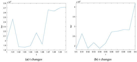
Figure 1.
The total number of iterations with different values of algorithmic parameters.
We then take , and choose r from the interval with a step size of . We present the total number of iterations (Iter) in Figure 1b as Algorithm 1 is used to solve all seven test problems with different sizes n (10, 50, 100 and 500) and different initial guesses (–). Figure 1b shows that Iter changes little when and Algorithm 1 with performs the best.
According to the above research, we take and , and compare Algorithm 1 (MSBFGS) with two similar algorithms proposed very recently to see which is more efficient as they are used to solve all seven test problems with different sizes n and different initial guesses. One is the Gauss–Newton-based BFGS method (GNBFGS for short) in [3] and another is MBFGS in [6] since they have been reported to be more efficient than the state-of-the-art ones.
In Table A1, we report the numerical performance of the three algorithms. For the simplification of statement, we use the following notations in Table A1.
P: the problems;
Dim: the dimension of test problems;
CPU: the CPU time in seconds;
Ni: the number of iterations;
Nf: the number of function evaluations;
Norm (F): the norm of at the stopping point;
F: a notation when an algorithm fails to achieve the given iteration tolerance, or in the limited number of iterations exceeds , or the MATLAB R2010b crashes, or in the limited the CPU time exceeds 100 s.
The underlined data in Table A1 indicate the superiority of Algorithm 1 in comparison with the others.
To further show the efficiency of the proposed method, we calculated the number of wins for the three algorithms in terms of the elapsed CPU time (CPU wins), the number of iterations (Iter wins) and the number of function evaluations (Nf wins) and we also calculated the failures (Fails) of the three algorithms. The results are recorded in Table 1.

Table 1.
Total number of wins or failures of algorithms.
In addition, we adopted the performance profiles introduced by Dolan and Moré [29] to evaluate the required number of iterations and the number of function evaluations.
It follows from the results in Table 1 and Figure 2 that our algorithm (MSBFGS) performs the best among the three algorithms, either with respect to the number of iterations, or with respect to the elapsed CPU time.
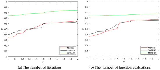
Figure 2.
Comparison of numerical performance among three methods.
In order to test the efficiency of the Algorithm 2 (MSBFGS2), we compared its performance for solving large-scale nonlinear symmetric equations with Algorithm 2.1 (NDDF) in [15] and Algorithm 2.1 (DFMPRP) in [13]. For the sake of fairness, we chose seven test problems, all from [15], where the relevant parameters of Algorithm 2 are same as those of NDDF in [15]. The values of parameters in DFMPRP are from [13]. The termination condition of all three algorithms is , or the number of iterations exceeds , or the MATLAB R2010b crashes, or the CPU time exceeds 100 s.
The numerical performance of all the algorithms is reported in Table A2 and Table A3. Table A2 shows the numerical performance of all three algorithms with the fixed initial points –. Table A3 demonstrates the numerical performance of all the three algorithms with initial points and randomly generated by Matlab’s Code “rand(n,1)” and “-rand(n,1)”, respectively. Furthermore, we calculated the “CPU wins”, the “Iter wins”, the “Nf wins” and the “Fails” of the three algorithms. The results are recorded in Table 2. We also adopted the performance profiles introduced by Dolan and Moré [29] to evaluate the required number of iterations and the required number of function evaluations of the three algorithms.
Table 2.
Total number of wins or failures of algorithms.
All the results of numerical performance in Figure 3 and Table 2, Table A2 and Table A3 demonstrate that our algorithm (MSBFGS2) performs better than the other two algorithms. MSBFGS2 is more efficient and robust than the others since the failures of MSBFGS2 are the least among the three algorithms in the case that different initial guesses are chosen.
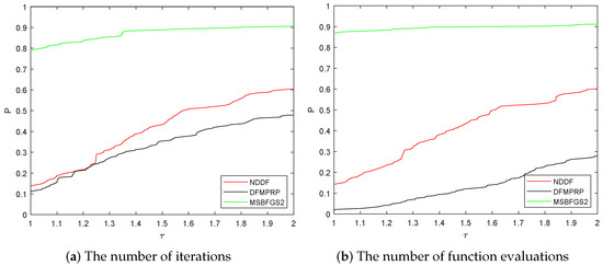
Figure 3.
Comparison of numerical performance among three methods.
5. Conclusions and Future Research
In this paper, we presented two derivative-free methods for solving nonlinear symmetric equations. For the first method, the direction is an approximate quasi-Newton direction and it can solve small-scale problems efficiently. For the second method, since it is not involved with the computation or storage of any matrix, it is applicable to solve the large scale system of nonlinear equations.
Global convergence theories of the developed algorithms were established. Compared with the similar algorithms, numerical tests demonstrated that our algorithms outperformed the others by costing less iterations, or less CPU time to find a solution with the same tolerance.
In future research, it would be valuable to deeply study the local convergence of the developed algorithms, in addition to the conducted analysis of global convergence in this paper. Additionally, our algorithms were designed only for the system of equations which is symmetric and satisfied with some relatively restrictive assumptions. Thus, it is interesting to study how to modify our algorithms to solve a more general system of equations.
Author Contributions
Z.W. conceived and designed the research plan and wrote the paper. J.G. performed the mathematical analysis, the development of the algorithm, experiments and wrote the paper. All authors have read and agreed to the published version of the manuscript.
Funding
This research is supported by the National Natural Science Foundation of China (Grant No. 71671190).
Institutional Review Board Statement
Not applicable.
Informed Consent Statement
Not applicable.
Data Availability Statement
The data used to support the findings of this study are available from the corresponding author upon request. All the computer codes used in this study are available from the corresponding author upon request.
Conflicts of Interest
The authors declare no conflict of interest.
Appendix A. Numerical Results
Table A1.
Numerical results of Problems 1–7.
Table A1.
Numerical results of Problems 1–7.
| P | dim | x0 | MBFGS | GNBFGS | MSBFGS | ||||||||||
|---|---|---|---|---|---|---|---|---|---|---|---|---|---|---|---|
| CPU | Ni | Nf | Norm (F) | CPU | Ni | Nf | Norm (F) | CPU | Ni | Nf | Norm (F) | ||||
| P1 | 10 | 0.0000 | 5 | 16 | 0.0000 | 4 | 13 | 0.0000 | 4 | 13 | |||||
| 0.0000 | 4 | 13 | 0.0156 | 4 | 13 | 0.0000 | 3 | 10 | |||||||
| 0.0000 | 11 | 51 | 0.0000 | 9 | 40 | 0.0624 | 120 | 604 | |||||||
| 0.0000 | 7 | 35 | 0.0000 | 9 | 31 | 0.0000 | 8 | 25 | |||||||
| 0.0000 | 5 | 16 | 0.0000 | 4 | 13 | 0.0000 | 4 | 13 | |||||||
| 0.0000 | 4 | 13 | 0.0000 | 4 | 13 | 0.0000 | 3 | 10 | |||||||
| 50 | 0.0936 | 5 | 16 | 0.0000 | 4 | 13 | 0.0000 | 4 | 13 | ||||||
| 0.0000 | 5 | 16 | 0.0000 | 4 | 13 | 0.0000 | 4 | 13 | |||||||
| 0.0780 | 11 | 54 | 0.0000 | 9 | 40 | 0.0780 | 120 | 604 | |||||||
| 0.0780 | 7 | 34 | 0.0000 | 9 | 31 | 0.0000 | 8 | 25 | |||||||
| 0.0000 | 3 | 10 | 0.0000 | 3 | 10 | 0.0000 | 3 | 10 | |||||||
| 0.0000 | 3 | 10 | 0.0000 | 3 | 10 | 0.0000 | 3 | 10 | |||||||
| 100 | 0.0312 | 5 | 16 | 0.0000 | 4 | 13 | 0.0000 | 4 | 13 | ||||||
| 0.0936 | 5 | 16 | 0.0000 | 4 | 13 | 0.0000 | 4 | 13 | |||||||
| 0.0000 | 10 | 39 | 0.0000 | 9 | 40 | 0.2808 | 120 | 604 | |||||||
| 0.0000 | 9 | 39 | 0.0000 | 9 | 31 | 0.0000 | 8 | 25 | |||||||
| 0.0000 | 3 | 10 | 0.0000 | 3 | 10 | 0.0000 | 2 | 7 | |||||||
| 0.0000 | 3 | 10 | 0.0000 | 3 | 10 | 0.0000 | 2 | 7 | |||||||
| 500 | 0.1092 | 5 | 16 | 0.1248 | 5 | 16 | 0.0780 | 4 | 13 | ||||||
| 0.1248 | 5 | 16 | 0.0780 | 4 | 13 | 0.0624 | 4 | 13 | |||||||
| 0.2028 | 9 | 40 | 0.2496 | 9 | 40 | 3.7128 | 120 | 604 | |||||||
| 0.2496 | 9 | 38 | 0.2496 | 9 | 31 | 0.2496 | 8 | 25 | |||||||
| 0.0624 | 2 | 7 | 0.0624 | 2 | 7 | 0.0000 | 2 | 7 | |||||||
| 0.0000 | 2 | 7 | 0.0312 | 2 | 7 | 0.0780 | 2 | 7 | |||||||
| P2 | 10 | 0.0312 | 3 | 10 | 0.0000 | 3 | 10 | 0.0000 | 2 | 7 | |||||
| 0.0000 | 3 | 10 | 0.0000 | 3 | 10 | 0.0000 | 2 | 7 | |||||||
| 0.0000 | 5 | 16 | 0.0000 | 5 | 16 | 0.0000 | 5 | 16 | |||||||
| 0.0000 | 5 | 16 | 0.0000 | 5 | 16 | 0.0000 | 5 | 16 | |||||||
| 0.0000 | 3 | 10 | 0.0000 | 3 | 10 | 0.0000 | 2 | 7 | |||||||
| 0.0000 | 3 | 10 | 0.0000 | 3 | 10 | 0.0000 | 2 | 7 | |||||||
| 50 | 0.0000 | 3 | 10 | 0.0000 | 3 | 10 | 0.0000 | 2 | 7 | ||||||
| 0.0000 | 3 | 10 | 0.0000 | 3 | 10 | 0.0000 | 2 | 7 | |||||||
| 0.0000 | 5 | 16 | 0.0000 | 5 | 16 | 0.0000 | 5 | 16 | |||||||
| 0.0000 | 5 | 16 | 0.0000 | 5 | 16 | 0.0936 | 5 | 16 | |||||||
| 0.0000 | 2 | 7 | 0.0000 | 2 | 7 | 0.0000 | 2 | 7 | |||||||
| 0.0000 | 2 | 7 | 0.0000 | 2 | 7 | 0.0000 | 2 | 7 | |||||||
| 100 | 0.0000 | 3 | 10 | 0.0000 | 3 | 10 | 0.0000 | 2 | 7 | ||||||
| 0.0000 | 3 | 10 | 0.0000 | 3 | 10 | 0.0000 | 2 | 7 | |||||||
| 0.0000 | 5 | 16 | 0.0000 | 5 | 16 | 0.0000 | 5 | 16 | |||||||
| 0.0780 | 5 | 16 | 0.0000 | 5 | 16 | 0.0000 | 5 | 16 | |||||||
| 0.0000 | 2 | 7 | 0.0000 | 2 | 7 | 0.0000 | 2 | 7 | |||||||
| 0.0000 | 2 | 7 | 0.0000 | 2 | 7 | 0.0000 | 2 | 7 | |||||||
| 500 | 0.1248 | 3 | 10 | 0.0624 | 3 | 10 | 0.0624 | 2 | 7 | ||||||
| 0.0624 | 3 | 10 | 0.2028 | 3 | 10 | 0.0936 | 2 | 7 | |||||||
| 0.2340 | 5 | 16 | 0.1560 | 5 | 16 | 0.1248 | 5 | 16 | |||||||
| 0.1248 | 5 | 16 | 0.0780 | 5 | 16 | 0.1248 | 5 | 16 | |||||||
| 0.0000 | 1 | 4 | 0.0624 | 1 | 4 | 0.0000 | 1 | 4 | |||||||
| 0.1092 | 1 | 4 | 0.0000 | 1 | 4 | 0.0000 | 1 | 4 | |||||||
| P3 | 10 | 0.0624 | 804 | 5068 | 0.1248 | 1182 | 7633 | 0.0468 | 78 | 331 | |||||
| 0.0312 | 281 | 1671 | 0.1092 | 1080 | 6918 | 0.0000 | 104 | 459 | |||||||
| 0.0468 | 134 | 624 | 0.0000 | 157 | 760 | 0.0000 | 36 | 109 | |||||||
| 0.0468 | 183 | 879 | 0.0936 | 739 | 4591 | 0.0000 | 65 | 250 | |||||||
| 0.0936 | 804 | 5068 | 0.1872 | 1182 | 7633 | 0.0000 | 78 | 331 | |||||||
| 0.0624 | 281 | 1671 | 0.1716 | 1080 | 6918 | 0.0000 | 104 | 459 | |||||||
| 50 | 1.3416 | 873 | 5489 | 1.8096 | 1317 | 8585 | 0.2028 | 118 | 566 | ||||||
| 0.0000 | 11 | 36 | 1.5288 | 1213 | 7782 | 0.2808 | 160 | 916 | |||||||
| 0.2028 | 130 | 592 | 0.2964 | 162 | 762 | 0.0936 | 37 | 112 | |||||||
| 0.1560 | 164 | 779 | 1.0764 | 762 | 4718 | 0.1872 | 151 | 736 | |||||||
| 0.0000 | 12 | 40 | 1.4820 | 1268 | 8228 | 0.1560 | 136 | 695 | |||||||
| 0.0000 | 12 | 39 | 1.5912 | 1238 | 8023 | 0.1872 | 152 | 809 | |||||||
| 100 | 3.6192 | 890 | 5605 | 5.4756 | 1349 | 8809 | 0.2808 | 77 | 305 | ||||||
| 0.0000 | 11 | 36 | 4.8048 | 1237 | 7932 | 0.3744 | 109 | 478 | |||||||
| 0.3744 | 134 | 610 | 0.5304 | 162 | 764 | 0.0624 | 37 | 112 | |||||||
| 0.5928 | 171 | 810 | 3.0576 | 777 | 4809 | 0.4212 | 113 | 514 | |||||||
| 0.0624 | 12 | 40 | 4.8516 | 1302 | 8446 | 0.1872 | 81 | 323 | |||||||
| 0.0624 | 12 | 40 | 5.1324 | 1301 | 8422 | 0.2964 | 84 | 346 | |||||||
| 500 | 38.6258 | 947 | 5970 | 60.1384 | 1428 | 9322 | 3.6816 | 91 | 376 | ||||||
| 15.2413 | 374 | 2253 | 54.5691 | 1313 | 8422 | 4.9764 | 131 | 615 | |||||||
| 5.4444 | 145 | 662 | 7.0200 | 176 | 827 | 1.2636 | 39 | 118 | |||||||
| 7.4412 | 179 | 856 | 34.4762 | 828 | 5128 | 1.2792 | 40 | 121 | |||||||
| 0.4524 | 12 | 40 | 59.2960 | 1371 | 8901 | 4.2900 | 104 | 454 | |||||||
| 0.4524 | 12 | 40 | 57.2368 | 1373 | 8892 | 4.1028 | 98 | 420 | |||||||
| P4 | 10 | 0.0000 | 34 | 157 | 0.0000 | 22 | 108 | 0.0000 | 52 | 361 | |||||
| 0.0000 | 26 | 113 | 0.0000 | 23 | 113 | 0.0468 | 40 | 274 | |||||||
| 0.0000 | 40 | 168 | 0.0000 | 73 | 479 | 0.0000 | 37 | 264 | |||||||
| 0.0000 | 44 | 178 | 0.0000 | 46 | 195 | 0.0000 | 53 | 377 | |||||||
| 0.0780 | 34 | 157 | 0.0000 | 22 | 108 | 0.0000 | 52 | 361 | |||||||
| 0.0000 | 26 | 113 | 0.0000 | 23 | 113 | 0.0000 | 40 | 274 | |||||||
| 50 | 0.0936 | 68 | 383 | 0.0624 | 64 | 370 | 0.0000 | 62 | 435 | ||||||
| 0.0000 | 66 | 364 | 0.0780 | 63 | 367 | 0.0000 | 40 | 274 | |||||||
| 0.1092 | 92 | 453 | 0.1248 | 123 | 790 | 0.0000 | 43 | 308 | |||||||
| 0.0624 | 94 | 487 | 0.1092 | 146 | 698 | 0.0624 | 48 | 347 | |||||||
| 0.0000 | 66 | 378 | 0.0780 | 65 | 383 | 0.0000 | 44 | 306 | |||||||
| 0.0624 | 66 | 378 | 0.0000 | 64 | 389 | 0.0468 | 38 | 264 | |||||||
| 100 | 0.0624 | 96 | 591 | 0.1404 | 94 | 574 | 0.0624 | 41 | 283 | ||||||
| 0.0624 | 99 | 591 | 0.1404 | 91 | 563 | 0.1092 | 40 | 279 | |||||||
| 0.1404 | 141 | 770 | 0.2808 | 203 | 1419 | 0.0000 | 47 | 332 | |||||||
| 0.2184 | 176 | 962 | 0.3120 | 204 | 1075 | 0.1092 | 51 | 368 | |||||||
| 0.1716 | 110 | 659 | 0.1092 | 86 | 543 | 0.0936 | 39 | 272 | |||||||
| 0.2340 | 125 | 710 | 0.0624 | 100 | 633 | 0.0780 | 41 | 287 | |||||||
| 500 | 3.2136 | 109 | 667 | 4.2432 | 138 | 842 | 1.2480 | 42 | 294 | ||||||
| 3.1044 | 107 | 644 | 3.1356 | 103 | 633 | 1.1700 | 44 | 310 | |||||||
| 7.4724 | 252 | 1549 | 12.8389 | 456 | 2833 | 1.2480 | 50 | 357 | |||||||
| 7.6596 | 259 | 1581 | 20.2801 | 653 | 3804 | 1.5288 | 47 | 348 | |||||||
| 3.1980 | 105 | 633 | 4.4772 | 151 | 962 | 1.0920 | 40 | 283 | |||||||
| 4.2432 | 162 | 983 | 3.1980 | 102 | 651 | 0.9828 | 38 | 265 | |||||||
| P5 | 10 | 0.0156 | 9 | 59 | 0.0000 | 9 | 59 | 0.0000 | 14 | 139 | |||||
| 0.0000 | 9 | 59 | 0.0000 | 9 | 59 | 0.0000 | 14 | 139 | |||||||
| 0.0000 | 11 | 72 | 0.0000 | 11 | 72 | 0.0000 | 15 | 149 | |||||||
| 0.0000 | 10 | 62 | 0.0000 | 10 | 62 | 0.0000 | 15 | 149 | |||||||
| 0.0000 | 9 | 59 | 0.0000 | 9 | 59 | 0.0000 | 14 | 139 | |||||||
| 0.0000 | 9 | 59 | 0.0000 | 9 | 59 | 0.0000 | 14 | 139 | |||||||
| 50 | 0.1248 | 37 | 280 | 0.0000 | 42 | 317 | 0.0000 | 18 | 177 | ||||||
| 0.0000 | 34 | 267 | 0.1248 | 34 | 267 | 0.0000 | 18 | 177 | |||||||
| 0.0000 | 50 | 380 | 0.1092 | 36 | 281 | 0.0000 | 18 | 177 | |||||||
| 0.0000 | 53 | 403 | 0.0000 | 37 | 285 | 0.0000 | 18 | 177 | |||||||
| 0.0000 | 34 | 267 | 0.0780 | 34 | 267 | 0.0000 | 17 | 167 | |||||||
| 0.0000 | 35 | 268 | 0.0000 | 35 | 268 | 0.0936 | 17 | 167 | |||||||
| 100 | 0.0624 | 79 | 610 | 0.0624 | 70 | 549 | 0.0624 | 19 | 187 | ||||||
| 0.1092 | 66 | 527 | 0.1092 | 69 | 539 | 0.0000 | 19 | 187 | |||||||
| 0.1716 | 78 | 610 | 0.1560 | 73 | 579 | 0.0000 | 19 | 187 | |||||||
| 0.1716 | 77 | 603 | 0.0624 | 84 | 654 | 0.0624 | 19 | 187 | |||||||
| 0.0936 | 65 | 517 | 0.1092 | 69 | 541 | 0.0624 | 15 | 147 | |||||||
| 0.0624 | 65 | 517 | 0.0624 | 65 | 517 | 0.0000 | 15 | 147 | |||||||
| 500 | 2.3400 | 81 | 662 | 2.3868 | 80 | 655 | 0.5304 | 20 | 196 | ||||||
| 2.2152 | 77 | 630 | 2.1216 | 79 | 648 | 0.5616 | 20 | 196 | |||||||
| 2.9484 | 98 | 800 | 2.8392 | 91 | 745 | 0.6084 | 22 | 216 | |||||||
| 2.8392 | 98 | 800 | 2.8236 | 91 | 745 | 0.6708 | 22 | 216 | |||||||
| 1.8408 | 59 | 482 | 2.1996 | 59 | 482 | 0.3588 | 11 | 107 | |||||||
| 1.8096 | 59 | 483 | 1.7940 | 59 | 483 | 0.3900 | 11 | 107 | |||||||
| P6 | 10 | 0.0000 | 108 | 484 | 0.0000 | 107 | 542 | 0.0468 | 267 | 2333 | |||||
| 0.0000 | 111 | 488 | 0.0468 | 125 | 640 | 0.0000 | 242 | 1940 | |||||||
| 0.0000 | 90 | 416 | 0.0000 | 52 | 220 | 0.0000 | 50 | 380 | |||||||
| F | F | F | F | 0.0312 | 222 | 1224 | 0.0000 | 287 | 2801 | ||||||
| 0.0312 | 108 | 484 | 0.0000 | 107 | 542 | 0.0000 | 267 | 2333 | |||||||
| 0.0156 | 111 | 488 | 0.0000 | 125 | 640 | 0.0000 | 242 | 1940 | |||||||
| 50 | 0.0624 | 148 | 789 | 0.0624 | 115 | 625 | 0.1092 | 141 | 1111 | ||||||
| 0.0624 | 139 | 740 | 0.0624 | 148 | 823 | 0.3588 | 569 | 4552 | |||||||
| 0.0624 | 113 | 611 | 0.0624 | 103 | 572 | 0.1716 | 280 | 2468 | |||||||
| F | F | F | F | 0.1092 | 195 | 1113 | 0.8268 | 1065 | 10678 | ||||||
| 0.1404 | 182 | 1028 | 0.0000 | 102 | 565 | 0.4524 | 684 | 5784 | |||||||
| 0.0624 | 99 | 554 | 0.0624 | 115 | 612 | 0.5928 | 942 | 7985 | |||||||
| 100 | 0.1248 | 187 | 1118 | 0.1716 | 160 | 999 | 0.2184 | 161 | 1315 | ||||||
| 0.2808 | 186 | 1151 | 0.2808 | 171 | 1031 | 0.6396 | 520 | 4163 | |||||||
| 0.2808 | 178 | 1058 | 0.1872 | 176 | 1049 | 0.4056 | 287 | 2537 | |||||||
| F | F | F | F | 0.4836 | 321 | 2078 | 4.8048 | 3042 | 35312 | ||||||
| 0.1248 | 160 | 974 | 0.2340 | 170 | 1022 | 1.4352 | 940 | 8407 | |||||||
| 0.1716 | 163 | 986 | 0.1716 | 170 | 1018 | 1.0296 | 915 | 7757 | |||||||
| 500 | 17.0509 | 576 | 4354 | 15.5377 | 538 | 3805 | 19.8433 | 662 | 5897 | ||||||
| F | F | F | F | 17.3317 | 559 | 4014 | 15.1945 | 490 | 3929 | ||||||
| 17.5345 | 558 | 3934 | 18.0961 | 548 | 3909 | 5.6472 | 181 | 1556 | |||||||
| F | F | F | F | 29.5934 | 961 | 8274 | F | F | F | F | |||||
| F | F | F | F | 16.2865 | 534 | 3793 | 14.1649 | 467 | 3744 | ||||||
| F | F | F | F | 16.5205 | 544 | 3847 | 13.5721 | 444 | 3564 | ||||||
| P7 | 10 | 0.0000 | 1 | 4 | 0.0000 | 1 | 4 | 0.0000 | 1 | 4 | |||||
| 0.0000 | 1 | 4 | 0.0000 | 1 | 4 | 0.0000 | 1 | 4 | |||||||
| 0.0000 | 0 | 1 | 0.0000 | 0 | 1 | 0.0000 | 0 | 1 | |||||||
| 0.0000 | 1 | 4 | 0.0000 | 1 | 4 | 0.0000 | 1 | 4 | |||||||
| 0.0000 | 1 | 4 | 0.0000 | 1 | 4 | 0.0000 | 1 | 4 | |||||||
| 0.0000 | 1 | 4 | 0.0000 | 1 | 4 | 0.0000 | 1 | 4 | |||||||
| 50 | 0.0000 | 1 | 4 | 0.0000 | 1 | 4 | 0.0000 | 1 | 4 | ||||||
| F | F | F | F | 0.0000 | 2 | 10 | 0.0000 | 2 | 7 | ||||||
| 0.0000 | 0 | 1 | 0.0000 | 0 | 1 | 0.0000 | 0 | 1 | |||||||
| F | F | F | F | 0.0000 | 4 | 24 | 0.0000 | 2 | 7 | ||||||
| 0.0000 | 1 | 4 | 0.0000 | 1 | 4 | 0.0000 | 1 | 4 | |||||||
| 0.0000 | 1 | 4 | 0.0000 | 1 | 4 | 0.0000 | 1 | 4 | |||||||
| 100 | F | F | F | F | 0.0000 | 4 | 18 | 0.0000 | 2 | 7 | |||||
| F | F | F | F | 0.0000 | 4 | 17 | 0.0000 | 2 | 7 | ||||||
| 0.0000 | 0 | 1 | 0.0000 | 0 | 1 | 0.0000 | 0 | 1 | |||||||
| F | F | F | F | 0.0000 | 4 | 26 | 0.0000 | 2 | 7 | ||||||
| 0.0000 | 2 | 7 | 0.0000 | 2 | 7 | 0.0000 | 2 | 7 | |||||||
| 0.0000 | 1 | 4 | 0.0000 | 1 | 4 | 0.0000 | 1 | 4 | |||||||
| 500 | F | F | F | F | 0.1248 | 4 | 23 | 0.0000 | 2 | 7 | |||||
| F | F | F | F | 0.0156 | 4 | 23 | 0.0468 | 2 | 7 | ||||||
| 0.0000 | 0 | 1 | 0.0000 | 0 | 1 | 0.0000 | 0 | 1 | |||||||
| F | F | F | F | 0.0936 | 4 | 30 | 0.0624 | 2 | 7 | ||||||
| 0.0624 | 3 | 10 | 0.0780 | 3 | 10 | 0.0780 | 2 | 7 | |||||||
| 0.1248 | 3 | 10 | 0.0156 | 3 | 10 | 0.0624 | 2 | 7 | |||||||
Table A2.
Numerical results of the 7 problems in [15] with fixed initial points.
Table A2.
Numerical results of the 7 problems in [15] with fixed initial points.
| P | dim | x0 | NDDF | DFMPRP | MSBFGS2 | |||||||||
|---|---|---|---|---|---|---|---|---|---|---|---|---|---|---|
| CPU | Ni | Nf | Norm (F) | CPU | Ni | Nf | Norm (F) | CPU | Ni | Nf | Norm (F) | |||
| P1 | 10000 | F | F | F | F | 0.1716 | 11 | 74 | 0.0624 | 3 | 11 | |||
| F | F | F | F | 0.0000 | 9 | 61 | 0.1092 | 3 | 11 | |||||
| F | F | F | F | F | F | F | F | 0.0000 | 8 | 31 | ||||
| F | F | F | F | 0.0624 | 10 | 71 | 0.0000 | 6 | 23 | |||||
| 0.0000 | 1 | 3 | 0.1092 | 5 | 33 | 0.0000 | 1 | 3 | ||||||
| 0.0000 | 1 | 3 | 0.0000 | 5 | 33 | 0.0000 | 1 | 3 | ||||||
| 100000 | F | F | F | F | 0.3744 | 12 | 81 | 0.0000 | 3 | 11 | ||||
| F | F | F | F | 0.2496 | 10 | 68 | 0.0000 | 3 | 11 | |||||
| F | F | F | F | F | F | F | F | 0.1404 | 8 | 31 | ||||
| F | F | F | F | 0.3744 | 11 | 78 | 0.1248 | 6 | 23 | |||||
| 0.0000 | 1 | 3 | 0.1872 | 4 | 26 | 0.0000 | 1 | 3 | ||||||
| 0.0000 | 1 | 3 | 0.1248 | 4 | 26 | 0.0312 | 1 | 3 | ||||||
| 500000 | F | F | F | F | 1.6536 | 12 | 81 | 0.1872 | 3 | 11 | ||||
| F | F | F | F | 1.6224 | 11 | 75 | 0.3276 | 3 | 11 | |||||
| F | F | F | F | F | F | F | F | 0.6396 | 8 | 31 | ||||
| F | F | F | F | 1.4664 | 11 | 78 | 0.3744 | 6 | 23 | |||||
| 0.0624 | 1 | 3 | 0.4524 | 4 | 26 | 0.0624 | 1 | 3 | ||||||
| 0.0468 | 1 | 3 | 0.5304 | 4 | 26 | 0.0624 | 1 | 3 | ||||||
| 1000000 | F | F | F | F | 3.0108 | 12 | 81 | 0.4368 | 3 | 11 | ||||
| F | F | F | F | 3.1356 | 11 | 75 | 0.4836 | 3 | 11 | |||||
| F | F | F | F | F | F | F | F | 1.0608 | 8 | 31 | ||||
| F | F | F | F | 3.2292 | 11 | 78 | 0.8268 | 6 | 23 | |||||
| 0.0624 | 1 | 3 | 0.7020 | 3 | 19 | 0.1404 | 1 | 3 | ||||||
| 0.1248 | 1 | 3 | 0.6864 | 3 | 19 | 0.1248 | 1 | 3 | ||||||
| P2 | 10000 | F | F | F | F | 0.1092 | 10 | 68 | 0.0000 | 2 | 7 | |||
| F | F | F | F | 0.0624 | 10 | 68 | 0.0000 | 2 | 7 | |||||
| F | F | F | F | 0.1872 | 12 | 83 | 0.0000 | 3 | 11 | |||||
| F | F | F | F | 0.1716 | 12 | 83 | 0.0000 | 3 | 11 | |||||
| 0.0000 | 1 | 3 | 0.0000 | 5 | 33 | 0.0000 | 1 | 3 | ||||||
| 0.0000 | 1 | 3 | 0.0000 | 5 | 33 | 0.0000 | 1 | 3 | ||||||
| 100000 | F | F | F | F | 0.3900 | 11 | 75 | 0.0156 | 2 | 7 | ||||
| F | F | F | F | 0.5460 | 11 | 75 | 0.0156 | 2 | 7 | |||||
| F | F | F | F | 0.4992 | 13 | 90 | 0.0780 | 3 | 11 | |||||
| F | F | F | F | 0.4836 | 13 | 90 | 0.0936 | 3 | 11 | |||||
| 0.0000 | 1 | 3 | 0.1560 | 4 | 26 | 0.0000 | 1 | 3 | ||||||
| 0.0624 | 1 | 3 | 0.0936 | 4 | 26 | 0.0000 | 1 | 3 | ||||||
| 500000 | F | F | F | F | 1.8720 | 12 | 82 | 0.0936 | 2 | 7 | ||||
| F | F | F | F | 1.7784 | 12 | 82 | 0.1404 | 2 | 7 | |||||
| F | F | F | F | 2.5428 | 13 | 90 | 0.3588 | 4 | 15 | |||||
| F | F | F | F | 2.9640 | 13 | 90 | 0.2496 | 4 | 15 | |||||
| 0.0312 | 1 | 3 | 0.7176 | 4 | 26 | 0.0156 | 1 | 3 | ||||||
| 0.0312 | 1 | 3 | 0.6396 | 4 | 26 | 0.0780 | 1 | 3 | ||||||
| 1000000 | F | F | F | F | 3.7440 | 12 | 82 | 0.2964 | 2 | 7 | ||||
| F | F | F | F | 3.9000 | 12 | 82 | 0.1560 | 2 | 7 | |||||
| F | F | F | F | 4.6956 | 14 | 97 | 0.6084 | 4 | 15 | |||||
| F | F | F | F | 4.4928 | 14 | 97 | 0.7332 | 4 | 15 | |||||
| 0.0468 | 1 | 3 | 1.0296 | 3 | 19 | 0.0468 | 1 | 3 | ||||||
| 0.0468 | 1 | 3 | 0.7176 | 3 | 19 | 0.1404 | 1 | 3 | ||||||
| P3 | 10000 | 0.3276 | 87 | 625 | 0.1560 | 48 | 498 | 0.3432 | 66 | 452 | ||||
| 0.2964 | 74 | 520 | 0.3900 | 56 | 573 | 0.1716 | 48 | 326 | ||||||
| F | F | F | F | F | F | F | F | 9.0325 | 2719 | 14327 | ||||
| F | F | F | F | F | F | F | F | F | F | F | F | |||
| 0.3276 | 79 | 563 | F | F | F | F | 0.1872 | 45 | 309 | |||||
| 0.3900 | 67 | 474 | F | F | F | F | 0.0468 | 35 | 242 | |||||
| 100000 | 2.2464 | 80 | 570 | 2.0748 | 53 | 553 | 1.5444 | 59 | 410 | |||||
| 2.3556 | 82 | 580 | 1.8096 | 47 | 485 | 1.3416 | 56 | 381 | ||||||
| F | F | F | F | F | F | F | F | 56.1448 | 2779 | 14670 | ||||
| F | F | F | F | F | F | F | F | F | F | F | F | |||
| 3.1200 | 106 | 761 | 2.5584 | 69 | 692 | 1.4352 | 57 | 392 | ||||||
| 2.2932 | 95 | 677 | 1.7628 | 52 | 536 | 1.0920 | 39 | 267 | ||||||
| 500000 | 10.1401 | 67 | 479 | F | F | F | F | 7.4412 | 55 | 385 | ||||
| 11.6065 | 74 | 520 | 9.3445 | 44 | 479 | 7.4880 | 53 | 366 | ||||||
| F | F | F | F | F | F | F | F | F | F | F | F | |||
| F | F | F | F | F | F | F | F | F | F | F | F | |||
| 10.6549 | 64 | 448 | 10.4521 | 52 | 548 | 3.6348 | 25 | 175 | ||||||
| 12.1525 | 79 | 554 | 11.1073 | 56 | 576 | 3.5880 | 25 | 175 | ||||||
| 1000000 | F | F | F | F | 22.1989 | 59 | 646 | 19.9369 | 73 | 505 | ||||
| 22.1053 | 80 | 563 | 29.4062 | 76 | 791 | 9.8125 | 39 | 268 | ||||||
| F | F | F | F | F | F | F | F | F | F | F | F | |||
| F | F | F | F | F | F | F | F | F | F | F | F | |||
| 21.8089 | 74 | 525 | 20.3893 | 56 | 568 | 15.1945 | 58 | 396 | ||||||
| 22.8073 | 75 | 530 | 20.9665 | 57 | 584 | 18.0025 | 63 | 434 | ||||||
| P4 | 10000 | 1.2324 | 102 | 716 | 0.4212 | 23 | 249 | 0.5304 | 31 | 210 | ||||
| 1.2324 | 99 | 716 | F | F | F | F | 0.3432 | 33 | 225 | |||||
| 0.6396 | 60 | 423 | F | F | F | F | 0.4836 | 48 | 337 | |||||
| 1.3728 | 109 | 767 | 0.9048 | 56 | 566 | 0.2652 | 23 | 162 | ||||||
| 0.7644 | 67 | 489 | 0.9360 | 56 | 563 | 0.3120 | 33 | 230 | ||||||
| 0.9048 | 69 | 503 | 0.7488 | 45 | 456 | 0.3120 | 29 | 201 | ||||||
| 100000 | 6.3336 | 145 | 1016 | 2.0280 | 29 | 308 | 0.8580 | 25 | 171 | |||||
| 4.3056 | 81 | 595 | F | F | F | F | 1.2168 | 26 | 185 | |||||
| 4.4148 | 94 | 672 | F | F | F | F | F | F | F | F | ||||
| 5.7096 | 133 | 941 | F | F | F | F | 10.6705 | 242 | 1693 | |||||
| 10.8109 | 236 | 1669 | 4.5396 | 76 | 743 | 1.0140 | 26 | 182 | ||||||
| 12.4801 | 278 | 1963 | 3.8376 | 61 | 588 | 1.3884 | 33 | 230 | ||||||
| 500000 | 18.7513 | 80 | 563 | 11.4037 | 36 | 382 | 5.1636 | 22 | 164 | |||||
| 27.3314 | 108 | 783 | F | F | F | F | 6.8484 | 34 | 243 | |||||
| 22.2457 | 104 | 727 | F | F | F | F | F | F | F | F | ||||
| 25.4438 | 108 | 772 | F | F | F | F | 9.5317 | 41 | 290 | |||||
| 16.0057 | 65 | 471 | 22.5421 | 83 | 787 | F | F | F | F | |||||
| 15.1477 | 65 | 471 | 29.6246 | 106 | 1001 | F | F | F | F | |||||
| 1000000 | 26.1146 | 58 | 396 | 18.0025 | 30 | 318 | 13.2289 | 30 | 214 | |||||
| 43.9299 | 88 | 641 | F | F | F | F | 35.1938 | 79 | 559 | |||||
| 50.0763 | 107 | 766 | F | F | F | F | F | F | F | F | ||||
| 41.1687 | 89 | 646 | F | F | F | F | 32.0894 | 76 | 544 | |||||
| F | F | F | F | 40.9815 | 71 | 696 | 15.9277 | 36 | 262 | |||||
| F | F | F | F | 46.7847 | 84 | 794 | 15.3193 | 33 | 243 | |||||
| P5 | 10000 | 0.1872 | 63 | 393 | 0.2808 | 57 | 523 | 0.1872 | 43 | 260 | ||||
| 0.1560 | 58 | 359 | 0.3276 | 51 | 482 | 0.2184 | 44 | 263 | ||||||
| 0.2184 | 66 | 416 | 0.3276 | 48 | 462 | 0.1092 | 46 | 279 | ||||||
| 0.2184 | 57 | 356 | 0.1716 | 56 | 529 | 0.0624 | 48 | 287 | ||||||
| 0.3276 | 59 | 372 | 0.2184 | 50 | 476 | 0.1716 | 46 | 277 | ||||||
| 0.2184 | 61 | 380 | 0.2808 | 56 | 528 | 0.2184 | 57 | 342 | ||||||
| 100000 | 1.1856 | 55 | 342 | 1.7628 | 54 | 505 | 1.1388 | 49 | 293 | |||||
| 1.3416 | 64 | 403 | 2.0124 | 70 | 652 | 0.9672 | 49 | 298 | ||||||
| 1.0764 | 55 | 351 | 1.7316 | 58 | 540 | 0.9360 | 40 | 244 | ||||||
| 1.0608 | 58 | 364 | 2.2152 | 72 | 664 | 1.0296 | 50 | 297 | ||||||
| 1.1232 | 54 | 345 | 1.8252 | 60 | 564 | 0.9828 | 44 | 266 | ||||||
| 1.1700 | 54 | 345 | 1.9188 | 58 | 546 | 1.1700 | 53 | 317 | ||||||
| 500000 | 9.8593 | 68 | 436 | 10.7173 | 58 | 544 | 6.3492 | 48 | 291 | |||||
| 7.3320 | 54 | 343 | 9.0325 | 53 | 509 | 6.6300 | 52 | 314 | ||||||
| 9.1573 | 61 | 390 | 9.3913 | 54 | 524 | 5.8968 | 49 | 297 | ||||||
| 9.1729 | 65 | 409 | 11.5753 | 59 | 554 | 6.1932 | 48 | 291 | ||||||
| 9.7501 | 70 | 446 | 10.0465 | 54 | 515 | 5.1480 | 46 | 274 | ||||||
| 10.0465 | 74 | 471 | 9.9061 | 54 | 510 | 5.3040 | 42 | 254 | ||||||
| 1000000 | 12.8545 | 47 | 300 | 19.2349 | 52 | 495 | 12.2617 | 47 | 285 | |||||
| 17.7529 | 64 | 404 | 19.4377 | 57 | 534 | 12.2773 | 47 | 284 | ||||||
| 16.5985 | 57 | 367 | 18.3145 | 53 | 514 | 9.7969 | 41 | 252 | ||||||
| 17.6437 | 58 | 365 | 21.3565 | 57 | 547 | 13.3381 | 53 | 321 | ||||||
| 16.5517 | 58 | 374 | 23.0569 | 61 | 574 | 10.7797 | 42 | 254 | ||||||
| 21.1069 | 73 | 470 | 17.9089 | 50 | 484 | 9.8437 | 48 | 290 | ||||||
| P6 | 10000 | 0.2340 | 29 | 356 | 0.3588 | 44 | 726 | 0.3120 | 25 | 302 | ||||
| 0.2028 | 18 | 249 | 0.2496 | 24 | 394 | 0.1716 | 27 | 331 | ||||||
| F | F | F | F | 0.4212 | 46 | 771 | 0.2184 | 31 | 389 | |||||
| 0.3900 | 39 | 496 | 0.2652 | 30 | 499 | 1.6380 | 178 | 2328 | ||||||
| 0.4368 | 61 | 714 | 0.3276 | 31 | 617 | 0.2808 | 28 | 345 | ||||||
| 0.3900 | 32 | 382 | 0.4368 | 33 | 658 | 0.2652 | 30 | 365 | ||||||
| 100000 | 2.7612 | 64 | 730 | 2.7612 | 45 | 745 | 1.4196 | 27 | 325 | |||||
| 1.2480 | 20 | 271 | 1.6224 | 26 | 428 | 1.6380 | 27 | 331 | ||||||
| F | F | F | F | 3.1356 | 51 | 859 | 1.4352 | 31 | 389 | |||||
| 1.5132 | 23 | 355 | 2.1528 | 32 | 531 | 10.3273 | 200 | 2614 | ||||||
| 1.5600 | 35 | 410 | 1.9968 | 26 | 516 | 1.5756 | 35 | 424 | ||||||
| 1.3260 | 23 | 297 | 2.3244 | 29 | 577 | 1.0920 | 23 | 286 | ||||||
| 500000 | 19.7497 | 69 | 785 | 17.2537 | 49 | 810 | 6.6924 | 28 | 337 | |||||
| 6.7392 | 21 | 282 | 8.3149 | 27 | 444 | 7.7688 | 28 | 343 | ||||||
| F | F | F | F | 16.5829 | 49 | 823 | 7.7532 | 31 | 389 | |||||
| 13.7281 | 37 | 510 | 10.5613 | 35 | 581 | 62.7748 | 215 | 2809 | ||||||
| 23.5874 | 74 | 915 | 11.6221 | 31 | 617 | 6.9420 | 23 | 287 | ||||||
| F | F | F | F | 14.5237 | 37 | 738 | 7.0356 | 24 | 298 | |||||
| 1000000 | 20.4517 | 37 | 441 | 28.8758 | 49 | 812 | 15.4285 | 29 | 347 | |||||
| 20.3425 | 37 | 436 | 15.5845 | 27 | 444 | 14.0089 | 29 | 355 | ||||||
| F | F | F | F | 32.1830 | 46 | 774 | 16.9105 | 31 | 389 | |||||
| F | F | F | F | 21.6217 | 37 | 613 | F | F | F | F | ||||
| 22.7137 | 40 | 463 | 25.9430 | 34 | 677 | 14.3365 | 27 | 332 | ||||||
| 60.4036 | 104 | 1197 | 25.8026 | 37 | 737 | 17.0353 | 32 | 390 | ||||||
| P7 | 10000 | 0.8580 | 115 | 1106 | 1.0452 | 94 | 1352 | 0.3276 | 63 | 572 | ||||
| 0.6864 | 115 | 1100 | 0.7956 | 78 | 1095 | 0.3276 | 51 | 470 | ||||||
| 0.8580 | 117 | 1106 | 1.7004 | 197 | 2809 | 0.6240 | 82 | 776 | ||||||
| 0.4992 | 83 | 789 | 0.7332 | 81 | 1127 | 0.2808 | 55 | 497 | ||||||
| 0.3276 | 44 | 422 | 0.3900 | 38 | 534 | 0.2028 | 28 | 261 | ||||||
| 0.2808 | 38 | 365 | 0.3120 | 35 | 490 | 0.2028 | 30 | 280 | ||||||
| 100000 | 3.5256 | 91 | 876 | 5.6472 | 119 | 1641 | 2.4960 | 73 | 669 | |||||
| 2.7144 | 70 | 664 | 3.9624 | 79 | 1090 | 1.7472 | 49 | 451 | ||||||
| 1.9812 | 54 | 507 | 10.4521 | 197 | 2921 | 2.6208 | 73 | 694 | ||||||
| 4.8984 | 129 | 1214 | 4.8204 | 101 | 1375 | 2.0436 | 54 | 493 | ||||||
| 1.7160 | 40 | 384 | 1.9188 | 34 | 478 | 0.9828 | 26 | 245 | ||||||
| 1.6692 | 40 | 384 | 1.7472 | 37 | 520 | 0.9204 | 25 | 235 | ||||||
| 500000 | 27.0818 | 122 | 1175 | 28.6418 | 115 | 1535 | 11.2321 | 59 | 539 | |||||
| 19.1257 | 88 | 844 | 29.9210 | 105 | 1502 | 11.2321 | 61 | 557 | ||||||
| 17.0041 | 78 | 732 | 67.8604 | 245 | 3540 | 13.7437 | 71 | 665 | ||||||
| 21.4345 | 93 | 863 | 35.8178 | 127 | 1817 | 12.7609 | 69 | 622 | ||||||
| 9.9061 | 41 | 394 | 13.4005 | 47 | 669 | 5.7252 | 26 | 245 | ||||||
| 10.2025 | 41 | 394 | 11.6065 | 44 | 623 | 5.4912 | 27 | 255 | ||||||
| 1000000 | 41.9331 | 98 | 946 | 64.8340 | 128 | 1775 | 20.9197 | 54 | 498 | |||||
| 50.1543 | 113 | 1081 | 38.2670 | 79 | 1022 | 22.9477 | 64 | 587 | ||||||
| 44.3355 | 107 | 1006 | F | F | F | F | 30.1238 | 80 | 762 | |||||
| 41.8083 | 101 | 940 | 64.4284 | 135 | 1839 | 19.0321 | 51 | 465 | ||||||
| 17.8933 | 43 | 413 | 19.9369 | 40 | 566 | 10.7797 | 26 | 245 | ||||||
| 18.3613 | 43 | 413 | 17.5501 | 35 | 504 | 9.8593 | 25 | 235 | ||||||
Table A3.
Numerical results of the 7 test problems in [15] with random initial guesses.
Table A3.
Numerical results of the 7 test problems in [15] with random initial guesses.
| P | dim | x0 | NDDF | DFMPRP | MSBFGS2 | |||||||||
|---|---|---|---|---|---|---|---|---|---|---|---|---|---|---|
| CPU | Ni | Nf | Norm (F) | CPU | Ni | Nf | Norm (F) | CPU | Ni | Nf | Norm (F) | |||
| P1 | 10000 | 0.1092 | 11 | 43 | F | F | F | F | 0.0624 | 6 | 23 | |||
| 0.0780 | 9 | 35 | 0.1092 | 11 | 78 | 0.0000 | 5 | 19 | ||||||
| 100000 | 0.2184 | 11 | 43 | F | F | F | F | 0.1560 | 7 | 27 | ||||
| 0.0936 | 9 | 35 | 0.3900 | 12 | 85 | 0.0624 | 5 | 19 | ||||||
| 500000 | 0.9204 | 11 | 43 | F | F | F | F | 0.3744 | 7 | 27 | ||||
| 0.6240 | 9 | 35 | 1.7784 | 12 | 85 | 0.3744 | 5 | 19 | ||||||
| 1000000 | 1.8720 | 11 | 43 | F | F | F | F | 1.0764 | 7 | 27 | ||||
| 1.3728 | 9 | 35 | 3.9000 | 12 | 85 | 0.7956 | 5 | 19 | ||||||
| P2 | 10000 | 0.0624 | 5 | 19 | 0.0624 | 11 | 76 | 0.0780 | 4 | 15 | ||||
| 0.0000 | 5 | 19 | 0.0780 | 11 | 76 | 0.0000 | 4 | 15 | ||||||
| 100000 | 0.1560 | 5 | 19 | 0.4680 | 12 | 83 | 0.0624 | 4 | 15 | |||||
| 0.1404 | 5 | 19 | 0.4368 | 12 | 83 | 0.0936 | 4 | 15 | ||||||
| 500000 | 0.3120 | 5 | 19 | 1.8876 | 13 | 90 | 0.4056 | 4 | 15 | |||||
| 0.2652 | 5 | 19 | 1.9188 | 13 | 90 | 0.2808 | 4 | 15 | ||||||
| 1000000 | 0.7176 | 5 | 19 | 3.3696 | 13 | 90 | 0.4836 | 4 | 15 | |||||
| 0.7020 | 5 | 19 | 3.2604 | 13 | 90 | 0.4368 | 4 | 15 | ||||||
| P3 | 10000 | F | F | F | F | F | F | F | F | F | F | F | F | |
| 0.3900 | 84 | 598 | F | F | F | F | 0.1872 | 44 | 305 | |||||
| 100000 | F | F | F | F | F | F | F | F | F | F | F | F | ||
| 1.6224 | 67 | 484 | F | F | F | F | 1.5132 | 61 | 418 | |||||
| 500000 | F | F | F | F | F | F | F | F | F | F | F | F | ||
| 8.8765 | 63 | 452 | F | F | F | F | 5.5536 | 42 | 293 | |||||
| 1000000 | F | F | F | F | F | F | F | F | F | F | F | F | ||
| 25.7714 | 78 | 562 | F | F | F | F | 13.4629 | 56 | 387 | |||||
| P4 | 10000 | 0.7176 | 63 | 470 | 0.4680 | 29 | 319 | 0.2964 | 27 | 193 | ||||
| 0.6396 | 45 | 325 | 1.1856 | 70 | 715 | 0.3120 | 31 | 210 | ||||||
| 100000 | 4.4148 | 102 | 753 | 2.5584 | 34 | 374 | 4.1652 | 102 | 713 | |||||
| 2.2464 | 57 | 411 | 11.1073 | 187 | 1632 | 1.6068 | 37 | 273 | ||||||
| 500000 | 36.5198 | 167 | 1221 | 9.2821 | 31 | 343 | 11.1385 | 54 | 385 | |||||
| 10.9669 | 51 | 369 | 45.9579 | 188 | 1703 | 19.6717 | 103 | 720 | ||||||
| 1000000 | F | F | F | F | 22.1677 | 35 | 386 | 23.7590 | 55 | 391 | ||||
| 38.5322 | 86 | 616 | F | F | F | F | 90.5274 | 215 | 1527 | |||||
| P5 | 10000 | 0.2652 | 81 | 495 | 0.3120 | 66 | 604 | 0.2808 | 70 | 414 | ||||
| 0.3276 | 83 | 512 | 0.2808 | 65 | 595 | 0.2808 | 82 | 487 | ||||||
| 100000 | 2.2152 | 113 | 695 | 2.4492 | 86 | 762 | 1.6224 | 78 | 468 | |||||
| 2.1216 | 104 | 638 | 1.9188 | 67 | 621 | 1.8876 | 90 | 530 | ||||||
| 500000 | 11.4817 | 94 | 577 | 10.6237 | 69 | 633 | 9.7033 | 88 | 521 | |||||
| 10.5301 | 87 | 533 | 12.3553 | 83 | 755 | 9.4537 | 88 | 523 | ||||||
| 1000000 | 20.9041 | 92 | 564 | 21.2161 | 75 | 696 | 18.4861 | 90 | 531 | |||||
| 25.8806 | 108 | 668 | 22.9009 | 77 | 712 | 17.9869 | 87 | 514 | ||||||
| P6 | 10000 | 1.3104 | 150 | 2015 | 0.9672 | 122 | 1897 | 0.2184 | 34 | 415 | ||||
| 0.2340 | 36 | 459 | 0.4368 | 36 | 599 | 0.1716 | 34 | 430 | ||||||
| 100000 | 9.1105 | 184 | 2547 | 11.7625 | 213 | 3364 | 1.3728 | 35 | 422 | |||||
| 3.9624 | 92 | 1151 | 1.8564 | 33 | 551 | 1.3104 | 27 | 335 | ||||||
| 500000 | 73.7105 | 255 | 3550 | F | F | F | F | 8.9389 | 41 | 487 | ||||
| 45.0219 | 153 | 2119 | 10.2493 | 35 | 583 | 8.0809 | 33 | 398 | ||||||
| 1000000 | 67.9384 | 107 | 1445 | F | F | F | F | 16.4737 | 37 | 449 | ||||
| 46.0047 | 82 | 1094 | 21.6061 | 42 | 695 | 13.9309 | 34 | 407 | ||||||
| P7 | 10000 | 0.5460 | 107 | 1006 | 1.8408 | 189 | 2772 | 0.4368 | 70 | 647 | ||||
| 0.5772 | 86 | 837 | 1.4664 | 173 | 2473 | 0.4056 | 80 | 749 | ||||||
| 100000 | 2.4024 | 72 | 681 | 17.5813 | 324 | 4944 | 1.9344 | 59 | 543 | |||||
| 3.9468 | 109 | 1114 | 15.0385 | 263 | 4219 | 3.3384 | 90 | 863 | ||||||
| 500000 | 16.7857 | 87 | 822 | F | F | F | F | 8.2369 | 48 | 450 | ||||
| 37.4714 | 162 | 1775 | F | F | F | F | 14.1025 | 73 | 712 | |||||
| 1000000 | 41.8083 | 108 | 1032 | F | F | F | F | 25.8650 | 80 | 746 | ||||
| 66.1444 | 134 | 1487 | F | F | F | F | 29.2970 | 84 | 827 | |||||
References
- Ortega, J.M.; Rheinboldt, W.C. Iterative Solution of Nonlinear Equations in Several Variables; Siam: Philadelphia, PA, USA, 1970. [Google Scholar]
- Sun, W.; Yuan, Y.X. Optimization Theory and Methods; Springer: Berlin/Heidelberg, Germany, 2006. [Google Scholar]
- Li, D.; Fukushima, M. A globally and superlinearly convergent Gauss-Newton based BFGS method for symmetric equations. SIAM J. Numer. Anal. 1999. [Google Scholar] [CrossRef]
- Gu, G.Z.; Li, D.H.; Qi, L.; Zhou, S.Z. Descent directions of quasi-Newton methods for symmetric nonlinear equations. SIAM J. Numer. Anal. 2002, 40, 1763–1774. [Google Scholar] [CrossRef]
- Li, D.H.; Fukushima, M. A modified BFGS method and its global convergence in nonconvex minimization. J. Comput. Appl. Math. 2001, 129, 15–35. [Google Scholar] [CrossRef]
- Zhou, W. A modified BFGS type quasi-Newton method with line search for symmetric nonlinear equations problems. J. Comput. Appl. Math. 2020, 367, 112454. [Google Scholar] [CrossRef]
- Wang, J.; Zhu, D. The inexact-newton via GMRES subspace method without line search technique for solving symmetric nonlinear equations. Appl. Numer. Math. 2016, 110, 174–189. [Google Scholar] [CrossRef]
- Yuan, G.L.; Yao, S.W. A BFGS algorithm for solving symmetric nonlinear equations. Optimization 2013, 62, 85–99. [Google Scholar] [CrossRef]
- Wang, X.L.; Li, D.H. A modified Fletcher-Reeves-type derivative-free method for symmetric nonlinear equations. Numer. Algebr. Control Optim. 2011, 1, 71–82. [Google Scholar]
- Zhang, L.; Zhou, W.; Li, D. Global convergence of a modified Fletcher-Reeves conjugate gradient method with Armijo-type line search. Numer. Math. 2006, 104, 561–572. [Google Scholar] [CrossRef]
- Dai, Y.H.; Kou, C.X. A nonlinear conjugate gradient algorithm with an optimal property and an improved Wolfe line search. SIAM J. Optim. 2013, 23, 296–320. [Google Scholar] [CrossRef]
- Xiao, Y.; Wu, C.; Wu, S.Y. Norm descent conjugate gradient methods for solving symmetric nonlinear equations. J. Glob. Optim. 2015, 62, 751–762. [Google Scholar] [CrossRef]
- Zhou, W.; Shen, D. Convergence properties of an iterative method for solving symmetric nonlinear equations. J. Optim. Theory Appl. 2015, 164, 277–289. [Google Scholar] [CrossRef]
- Zhang, L.; Zhou, W.; Li, D.H. A descent modified Polak-Ribière-Polyak conjugate gradient method and its global convergence. IMA J. Numer. Anal. 2006, 26, 629–640. [Google Scholar] [CrossRef]
- Liu, J.K.; Feng, Y.M. A norm descent derivative-free algorithm for solving large-scale nonlinear symmetric equations. J. Comput. Appl. Math. 2018, 344, 89–99. [Google Scholar] [CrossRef]
- Liu, J.K.; Li, S.J. New three-term conjugate gradient method with guaranteed global convergence. Int. J. Comput. Math. 2014, 91, 1744–1754. [Google Scholar] [CrossRef]
- Cheng, W.Y.; Chen, Z.X. Nonmonotone spectral method for large-scale symmetric nonlinear equations. Numer. Algorithms 2013, 62, 149–162. [Google Scholar] [CrossRef]
- Yusuf, W.M.; Sabiu, J. A derivative-free conjugate gradient method and its global convergence for solving symmetric nonlinear equations. Int. J. Math. Math. Sci. 2015, 2015, 1–8. [Google Scholar]
- Zhou, W.J.; Chen, X.L. On the convergence of a derivative-free HS type method for symmetric nonlinear equations. Adv. Model.Optim. 2012, 3, 645–654. [Google Scholar]
- Yakubu, U.A.; Mamat, M. A recent modification on dai-liao conjugate gradient method for solving symmetric nonlinear equations. Far East J. Math. Sci. 2018, 103, 1961–1974. [Google Scholar] [CrossRef]
- Lv, J.; Deng, S.; Wan, Z. An efficient single-parameter scaling memoryless Broyden-Fletcher-Goldfarb-Shanno algorithm for solving large scale unconstrained optimization problems. IEEE Access 2020, 8, 85664–85674. [Google Scholar] [CrossRef]
- Zhou, W.J.; Zhang, L. A nonlinear conjugate gradient method based on the MBFGS secant condition. Optim. Methods Softw. 2006, 21, 707–714. [Google Scholar] [CrossRef]
- Byrd, R.H.; Nocedal, J. A tool for the analysis of quasi-Newton methods with application to unconstrained minimization. SIAM J. Numer. Anal. 1989, 26, 727–739. [Google Scholar] [CrossRef]
- Dennis, J.E. A characterization of superlinear convergence and its application to quasi-Newton methods. Math. Comput. 1974, 28, 549–560. [Google Scholar] [CrossRef]
- Li, Q.; Li, D.H. A class of derivative-free methods for large-scale nonlinear monotone equations. IMA J. Numer. Anal. 2011, 31, 1625–1635. [Google Scholar] [CrossRef]
- Raydan, M. The Barzilai and Borwein gradient method for the large scale unconstrained minimization problem. SIAM J. Optim. 1997, 7, 26–33. [Google Scholar] [CrossRef]
- Kelley, C.T. Iterative methods for linear and nonlinear equations. Front. Appl. Math. 1995, 16, 206–207. [Google Scholar]
- Yamakawa, E.; Fukushima, M. Testing parallel variable transformation. Comput. Optim. Appl. 1999, 13, 253–274. [Google Scholar] [CrossRef]
- Dolan, E.D.; Moré, J.J. Benchmarking optimization software with performance profiles. Math. Program. 2002, 91, 201–213. [Google Scholar] [CrossRef]


Publisher’s Note: MDPI stays neutral with regard to jurisdictional claims in published maps and institutional affiliations. |
© 2021 by the authors. Licensee MDPI, Basel, Switzerland. This article is an open access article distributed under the terms and conditions of the Creative Commons Attribution (CC BY) license (https://creativecommons.org/licenses/by/4.0/).