Abstract
The goal of clustering is to identify common structures in a data set by forming groups of homogeneous objects. The observed characteristics of many economic time series motivated the development of classes of distributions that can accommodate properties, such as heavy tails and skewness. Thanks to its flexibility, the skewed exponential power distribution (also called skewed generalized error distribution) ensures a unified and general framework for clustering possibly skewed and heavy tailed time series. This paper develops a clustering procedure of model-based type, assuming that the time series are generated by the same underlying probability distribution but with different parameters. Moreover, we propose to optimally combine the estimated parameters to form the clusters with an entropy weighing k-means approach. The usefulness of the proposal is shown by means of application to financial time series, demonstrating also how the obtained clusters can be used to form portfolio of stocks.
1. Introduction
The goal of clustering is to identify common structures in a data set by forming groups of homogeneous data. This objective can be achieved by minimizing the within-group similarity and by maximizing the between-group dissimilarity.
Clustering of time series data is an important tool for data analysis in different areas ranging from engineering to finance and economics. For example, through clustering methods it is possible to build portfolios of similar stocks for financial applications (for example [1,2,3]). The main clustering approaches for time series can be summarized into three main groups [4]: observation-based, feature-based, and model-based.
In the observation-based clustering the raw data are clustered according to a specified distance measure. Several authors proposed fuzzy extensions of common clustering algorithms for raw data (for example [5,6,7,8,9]). The time series involved could have either the same length or not. In the second case, it is common to take advantage of the dynamic time warping (DTW) technique that is used to find an optimal alignment between two series with different lengths. (for example [9,10]).
In the feature-based clustering, the objects are clustered according to some of the data’s features. The main advantage of this class of clustering approaches lies in the fact that the time series length is not an issue because objects with different length can be clustered together. Common time series features considered for clustering are the autocorrelation function (ACF) [11,12], the partial autocorrelation function (PACF) [13], the features of wavelet decomposition of the time series (for example [14,15]) or the cepstral (for example [16,17]).
The model-based clustering approaches assume, instead, that the time series are generated by the same statistical model (for example [18,19,20,21]) or that they have the same probability distribution (for example [22,23]). The spirit of most of the model-based clustering procedures is to group objects according to the estimated parameters. Important examples are the clustering methods based on ARMA process distances (for example [18,19,24]), GARCH-based distances for heteroskedastic time series [19,20,25], estimates of the probability distributions’ parameters (for example [22,23]) or, more recently, conditional higher moments (for example see [26]).
This paper develops a clustering procedure of the model-based type, assuming that the time series are generated by the same underlying probability distribution but with different parameters. Clearly, with this aim the specification of a very general distribution is required in order to account for a wide range of possible special cases.
The observed characteristics of many financial and economic time series motivated the development of a family of distributions that are enough flexible to accommodate skewness and heavy-tails, while nesting symmetric and bell-shaped distributions (e.g., the Normal) as special cases.
An important desired property of these classes is that the maximum likelihood estimation of the parameters is possible. A class of asymmetric distributions with the desired properties of accommodating heavy tails and skewness is represented by the skewed exponential power distribution (SEPD) [27,28,29,30]. It generalizes the exponential power distribution (also called generalized error distribution, GED) for skewness.
Many financial applications of the GED, as well as its skewed extensions, have been considered (for example [29,30,31,32,33,34,35,36,37,38]). For example, [30] explored moments (also see [29]) as well as measures, such as value at risk and expected shortfall that are useful in financial applications. Similarly, [37] proposed a GED-based value at risk model, while [38,39] studied the role of the Skewed GED in forecasting volatility.
In general, the exponential power distribution, either symmetric or not, encompasses a very wide variety of special cases. Examples are the Gaussian, the skewed normal, the Laplace, the skewed Laplace distribution, and many others [37,40,41,42].
Therefore, in what follows, we consider the skewed exponential power distribution family as the underlying assumption for all the considered time series. Thanks to its flexibility it ensures a unified and general framework for clustering possibly skewed time series.
The paper is structured as follows. In the next section, the entropy weighted clustering algorithm based on the skewed exponential power distribution is discussed. To show the usefulness of the proposed approach we provide two applications to different financial datasets in the Section 4. Then, in the Section 5 we propose to use the clusters obtained in the Section 4 to build a portfolio of stocks. At the end some conclusions are offered.
2. The SEPD-Based Clustering Approach
A very general and flexible family of distribution is represented by the exponential power distribution (also called generalized error distribution or exponential power function). The EPD random variable Z has the following probability density function [42,43]:
where , is called location parameter, is called scale parameter, is a measure of fatness of tails and is called shape parameter (see [40]) and is the Gamma function. By construction, this distribution is symmetric and does not allow for skewness (Figure 1).
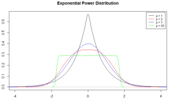
Figure 1.
Exponential power distribution for different values of shape.
It is possible to write the EPD probability density (1) in more compact form by means of [40]:
where C is a normalizing constant. The shape parameter p defines the heavy-tailedness of the distribution. Hence, with a small value of p we obtain more flat distribution and vice-versa with a large p.
A very important feature of the EPD is that it includes many common distributions as special cases, depending by the value of shape parameter p (Figure 1).
In particular, the Gaussian distribution is a special case when , and when the distribution has fatter tails than a Gaussian distribution [37]. Moreover, when we have a Laplace distribution, and for we have the uniform distribution [42].
Important contributions that extended the exponential power distribution for skewness are represented by [27,28], where an additional skewness parameter, denoted in this paper, is introduced. (see Figure 2).
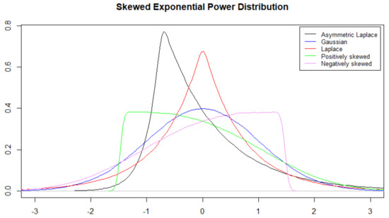
Figure 2.
Skewed exponential power distribution for different values of shape and skewness.
Some papers (for example [29,30,34,40]) constructed seemingly different classes of SEPD distributions. However, as suggested by [40], all of them are actually reparametrizations of the SEPD proposed by [27,28].
In this paper, following [34], we say that a random variable Z has a skewed exponential power distribution if its probability density function is the following:
where:
The parameters and correspond to location and scale, respectively, while controls skewness, and p is the shape parameter. For , the distribution is symmetric about so we obtain the symmetric exponential power distribution. In the case , by letting we obtain the skewed Laplace distribution with density [34]:
For and , instead, we obtain the skewed normal distribution as defined in [44]. More details about the SEPD and the skewed Laplace distribution can be found in [34].
The great flexibility of the SEPD can be successfully exploited in the clustering process if the aim is to form distribution-based clusters. Distribution-based clustering could be of interest for a variety of applications (for example [22,23]).
In what follows, following in the spirit the contribution of [23], we propose a clustering algorithm that uses the estimated moments from the skewed exponential power distribution here introduced to form clusters. In other words, time series with similar estimated parameters are be placed in the same cluster. Moreover, since the underlying distribution has more than one parameter, following [7,45], we propose to optimally weight each parameter that represents a different feature of the data distribution.
The clustering model can be presented as follows. Let’s assume to have time series that are generated by a skewed exponential power distribution of parameters , and . We can store the estimated parameters in the following matrix:
that we can be used to compute the time series’ dissimilarities.
As briefly stated before, since the SEPD has more than one parameter, a natural question is how would we use this information. Indeed, it is surely possible to cluster the time series only according to the location estimates or with respect to the scale parameter. Similarly, we can be interested in clustering time series with similar skewness or shape.
In this paper, we do not cluster the time series according to a single parameter but, instead, we aim to optimally combine them.
A useful approach for optimally weighting different features is represented by the weighted k-means (WKM) algorithm of [46]. The WKM algorithm proposes to incorporate a weighted distance function within the usual k-means algorithm. The main idea is that the weights are a measure of the relative importance of each feature with respect to the membership of the observations to a given cluster.
Formally, the weighted k-means algorithm (WKM) can be formalized as follows:
under the constraints:
where is binary and takes value of 1 if the n-th object belongs to the c-th cluster, represents the weight of the m-th feature in determining the c-th cluster and , represents the (euclidean) distance between the m-th feature of the n-th time series and the one of the c-th centroid.
Applied to the context of the distribution-based clustering, the weights are suitable values associated to each parameter m in the matrix shown in (5) of the specified distribution within the c-th cluster.
Note that the weight is intrinsically associated with the squared distance for the specified distribution parameters. This makes possible to optimally weighting each distribution’s feature in calculating the dissimilarities. Moreover, another appealing feature is that each c-th group has its own optimal weight vector.
Then, the exponent has to be analyzed. With we obtain the usual k-means clustering algorithm, while with a value of , we have that the weights associated to the feature with the smallest value of the weighted dissimilarity is equal to 1 and all the others are equal to zero.
When , the larger the , the smaller the weight . With a , we have that the larger the larger the weight . Then, if the larger the features’ dissimilarity, the larger is the weight and this is against the variable weighting principal [46].
Therefore, we cannot choose , or but in the WKM algorithm suitable values are or .
However, the exponent is an artificial device, lacking a strong theoretical justification [7]. Note that the value of in the Formula (6) is similar to the fuzziness parameter in the fuzzy c-means algorithm. To overcome this problem, the usage of a regularization term has been proposed [7,45]. In this case, the burden represented by is shifted to the regularization term obtaining, in such a way, a factor that multiplies the regularization contribution to the clusters formation.
With this respect, [45] proposed a clustering algorithm where the weight of a given feature in a cluster represents the relevance of each feature in determining the clusters.
Therefore, [45] modified the objective function (6) by adding the weight entropy term such that, at the same time, we minimize the within cluster dispersion and maximize the negative weight entropy. Hence, we force more features to contribute in the formation of the groups [47].
The new objective function can be written as follows:
subject to the constraints:
where is binary, if a hard clustering procedure is developed, and takes value of 1 if the n-th object belongs to the c-th cluster, represents the weight of the m-th feature in determining the c-th cluster and , represents the (euclidean) distance between the m-th feature in the matrix shown in (5) of the n-th time series and the one of the c-th centroid.
The first term in (9) is the sum of the within cluster dispersion, while the other one is the negative weight entropy. The positive parameter controls for the size of the weights, meaning that with we decide the degree of discrimination between the features [45].
The algorithm works as follows. An initial set of k means are identified as the starting centroids. An initial cluster is defined considering that the observations are clustered to the nearest centroid according to the euclidean distance measure among distribution parameter estimates (5). The centroids are identified based on these clusters, while the weights are computed for each time series in any given cluster. Then, we compute the new centroids and, by using an updated weighted distance, each time series is clustered to its nearest new centroid. These steps are repeated until the algorithm converges.
In the case of skewed exponential power distribution, the optimal weights of the SEPD-DWEKM model, obtained by the solution of the optimization problem (9), are equal to:
The proof of (12) can easily be derived by following [46]. Similarly to the standard k-means algorithm is updated as follows:
where means that the n-th object is assigned to the c-th cluster, so we have an hard, not fuzzy, final assignment. If a time series is equidistant from two clusters, we assign it to the one with the smallest index.
From (12) we understand the role played by the parameter , that is used to control for the size of the weights. Indeed, if , the weights are inversely proportional to squared distance . Therefore, the smaller , the larger the weights and, hence, the more important the corresponding dimension m. Instead, if , the weights is proportional to the distance . Therefore, the larger the distance is the larger is the associated weight. This is a contradictory result and, hence, cannot be smaller than zero. In the end, can be set equal to zero. In this case, the dimension with the smallest distance has a weight equal to 1, , while all the others are zero . Therefore, each cluster contains only one important dimension.
A final crucial aspect of the any clustering procedure is the selection of the number of clusters (C). With this respect we compute the silhouette width criterion (SWC) of [48]. Clearly, the best partition is expected to be pointed out when the SWC are maximized, which implies the minimization of the intra-group distance the maximization of the inter-group distance.
3. Application to Financial Time Series
To show the effectiveness of the proposed clustering approach, in what follows we provide an application to stock market data. The role of skewness and kurtosis in modeling financial data is well documented (for a review see [49]).
Therefore, financial market data represent a clear example of the possible application since the empirical densities of the financial time series are proven to be non-Gaussian, asymmetric, and heavy tailed [50] (We have to highlight that this statement is not always true. For example, it is known that most of monthly stock indices, with low frequencies, show a behavior according to a Gaussian distribution. However, it is similarly accepted that daily stock returns are not normally heavy-tailed and asymmetrically distributed. Therefore, in this paper we deal with daily returns data).
In what follows we provide empirical applications of the proposed clustering approach to two different financial datasets. In the first experiment, we consider the FTSE100’s stocks, while in the second we consider the industrial sector’s stocks belonging to the S&P500 index.
3.1. FTSE100 Stocks
The first application with real data aims to cluster the stocks belonging to the FTSE100 index. With this aim we consider the daily stock returns over the last 10 years, from the 1 January 2011 to the 1 January 2021 (Figure 3).
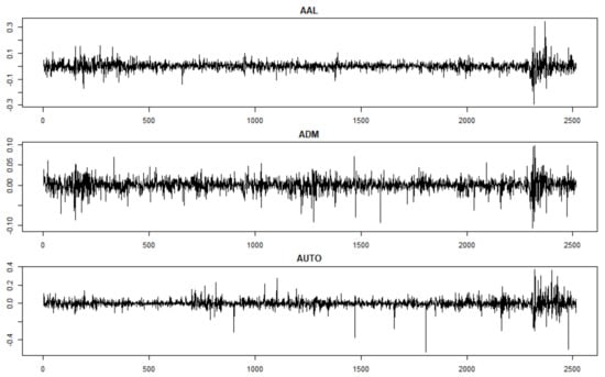
Figure 3.
Sample of stock returns time series included in the dastaset under consideration (FTSE100 data).
In particular, over the 100 stocks we selected those without missing values within the considered sampling period, hence getting as result stocks. The list of the stocks included in the sample is shown in Table A1 in the Appendix A.
To empirically motivate the peculiar distributional characteristics of the stock returns included in the sample, we show some estimated empirical densities (Figure 4).
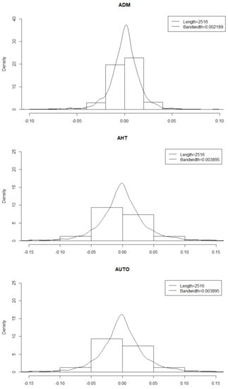
Figure 4.
Empirical densities of the stocks shown in Figure 3.
Moreover, in Table 1 we report the sample estimators for mean, standard deviation, skewness, and kurtosis, as well as the Jarque-Bera [51] normality test. The results of the conducted normality tests suggest to reject the null hypothesis of normal distribution for all the stocks (see JB test column of Table 1). Accordingly, it can be highlighted that any stock shows a symmetric distribution and the majority of them are negatively skewed. Furthermore, the stocks show very high leptokurtic distributions with fatter tails than the Gaussian. Indeed, within the sample only one stock shows a kurtosis lower than 3 (i.e., IAG) while all the others have much higher values.

Table 1.
Descriptive statistics and normality test of Jarque-Bera [51] for the FTSE100 stocks.
Therefore, for clustering time series with similar distributions we use the approach based on the skewed exponential power distribution presented in the previous section. The first step of the clustering procedure requires the estimation of the SEPD’s parameters. Then, the number of clusters has to be chosen.
At this aim, we consider the average silhouette width criterion (SWC). In Figure 5 is reported the final result.
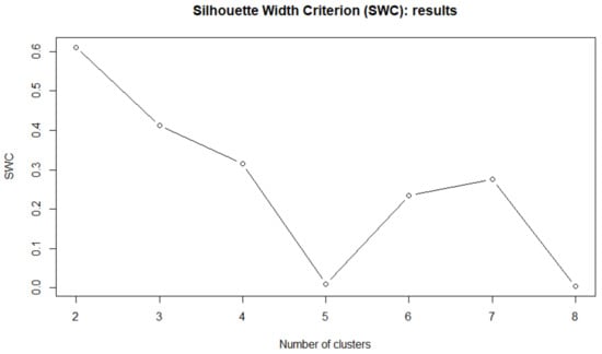
Figure 5.
Silhouette width criterion for different number of clusters C (distribution-based clustering)—experiment with FTSE100 stocks.
Accordingly, the parameters estimated by maximum likelihood (MLE) (We use the R environment to obtain the parameter estimates. More in details, the function nlminb is used in order to maximize the log-likelihood function of the SEPD. As starting values for the function we use the sample estimates for location and scale parameters, while we set and (symmetric distribution) for shape and skewness, respectively, such that the starting values correspond to the normal distribution, as well as the final clustering results are reported in Table 2.
Table 2.
MLE parameters estimation from a SEPD and assigned clusters according to the Entropy Weighting K-means–FTSE100 data.
From Table 2 is evident that the second cluster contains the majority of the stocks. Moreover, the two groups mainly differentiate each other in terms of their shapes. Indeed, in the second cluster we have the stocks characterized by the lowest shape parameters p and by a skewness parameter always greater than 1. In general, sorting by shape is, in this case, more informative than sorting by the degree of skewness that, however, still reveals important information about the distribution of the stocks placed within each group.
Moreover, some additional comments about data heterogeneity within each cluster can be provided by looking at Table 2. Indeed, the second cluster seems to be the one with the highest degree of heterogeneity. To see why, we can look at the column of the estimated skewness in Table 2. Although in the first cluster we have all values of close to 1, in the case of cluster 2 the values range from to . A similar discussion can be provided for the shape values p, since in the cluster 1 all the stocks have low shape’s parameters p.
In general, the weights obtained by means of the entropy weighted k-means algorithm (EKWM) reflect, as discussed in the previous section, this heterogeneity. Indeed, the weights are inversely proportional to squared distances such that to small distances are associated larger weights.
Table 3 shows the optimal weights computed with respect to the selected clusters. According to the arguments presented so far, the weights effectively reflect the degree of heterogeneity of the features. Indeed, in the cluster 2 the shape’s weight is the lowest one since the distances in terms of shape parameters in the second cluster are higher than the same shape-based distances in the first cluster.
Table 3.
Distribution-based Entropy Weighting K-means for FTSE100 stocks: resulting weights.
In the case of other parameters (i.e., location, scale, and skewness) the weights assigned in the two groups are very similar. In other words, the Table 3 highlights that the two clusters mainly differentiate each other because of the distribution’s shape.
However, one can ask whether a distribution-based clustering approach for time series is more convenient than other common approaches available. Clearly there is not an easy answer to this question since the usefulness of a clustering approach depends by its aim and by the researcher’s goal.
However, in what follows we provide an in-sample comparison of a well-established clustering approach for financial time series based on the stock returns correlations (e.g., see [1]). In particular, assuming a k-medoids approach, we cluster the time series according to the following correlation-based distance:
that depends by the correlation between the n-th stock returns and the j-th returns . In Figure 6 is reported the SWC criterion for different clusters C. The number of clusters with highest validity are .
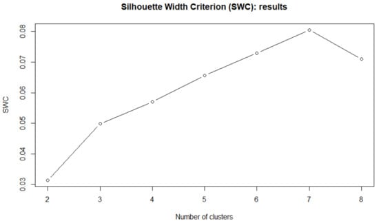
Figure 6.
Silhouette width criterion for different number of clusters (correlation based clustering)—experiment with the FTSE100 stocks.
However the highest SWC is equal to 0.08 and is dramatically lower than the SWC value in Figure 5 that is equal to 0.6. The differences between the two classifications are shown in Table 4.
Table 4.
Differences in the classification between the entropy weighted distribution-based and the correlation-based clustering approaches—FTSE100 data.
In general, according to the SWC criterion, we can argue that the clusters obtained by means of the distribution-based approach are much more accurate than those obtained with a correlation-based approach, that is well established in finance.
3.2. S&P500 Stocks: Industrial Sector
As additional experiment we also select the stock prices of the companies belonging to the industrial sector that are included in the S&P500 Index. In more detail, we downloaded the last 10 years of daily observations for all the 74 stocks quoted, specifically from the 1 January 2011 to 1 January 2021.
The considered stocks have different lengths because some of them have been quoted later. Differently from the previous experiment, we now decide to consider in the sample also the stocks with different lengths, thus containing missing values.
Indeed, as the proposed approach is of model-based type, we are able to cluster two time series with different length as far they share a similar distribution. Indeed, in the sample there are also stocks with a length as in the case of CARR and OTIS.
The entire list of the stocks considered in the sample, with their length, is shown in the Table A2. Particularly, for each time series we consider the logarithmic returns (Figure 7).
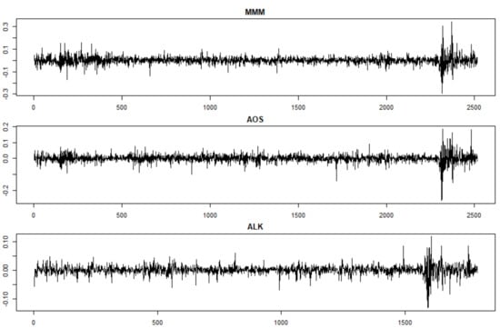
Figure 7.
Sample of stock returns time series included in the dataset under consideration (S&P500 data).
As in the previous experiment, in order to empirically show the aforementioned stock returns characteristics (i.e., heavy tails and skewness) in Figure 8 are reported the empirical densities for the sample of stock returns also shown in Figure 7.
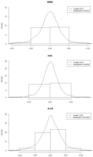
Figure 8.
Empirical densities of the stocks shown in Figure 7.
From Figure 8 it is possible to note that the considered time series show very different distributions, as well as a strong deviation from Gaussianity. Moreover, we also report in Table 5 the main descriptive statistics, as well as the [51] test of normality. In general, from these simple considerations appear clearly the need for the specification of a very flexible distribution able to accurately capture these differences.
Table 5.
Descriptive statistics and normality test of Jarque-Bera [51] for the S&P500 stocks.
As previously described, the first step of the proposed clustering procedure involves the estimation of the skewed exponential power distribution parameters (i.e., location, scale, skewness and shape) by means of maximum likelihood method. Then, as usual, the second step of the procedure involves the decision about the number of clusters C.
As previously specified, we take advantage of the silhouette width criterion (SWC), whose results are shown in the Figure 9.
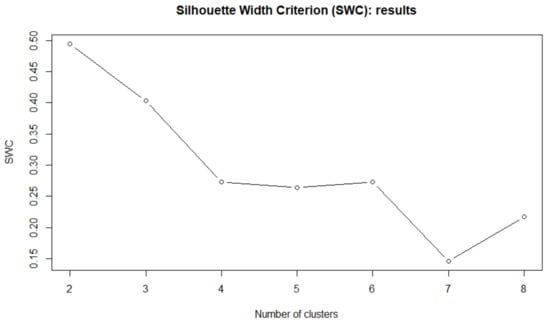
Figure 9.
Silhouette width criterion for different number of clusters C (distribution-based clustering)—S&P500 stocks.
The highest value of the silhouette is obtained with clusters. Then, from the distribution (SEPD)-based entropy weighting k-Means (SEPD-EWKM) algorithm we obtain the hard partition shown in Table 6.
Table 6.
MLE estimates of a skewed exponential power distribution and the entropy weighting clustering results—S&P500 data.
As in the previous experiment, the two resulting clusters are not balanced since the second cluster contains most of the stocks in the sample. Moreover, it appears clearly that the two clusters differentiate each other in terms of shape. Indeed, the first cluster contains all the stocks with shape parameter p lower than , while on the other side in the second one we have all the stocks with higher shape’s parameters.
However, additionally, the skewness allows a remarkable distinction among the two clusters since in the first group we find most of the stocks with while in the second one the stocks with a lower degree of skewness. Nevertheless, the heterogeneity in terms of skewness in the first cluster appear considerable.
Heterogeneity can also be analyzed by means of the features’ weights that show at the same time the relative importance of each estimated parameter in determining the cluster’s composition. The optimal weights for this experiment are reported in Table 7.
Table 7.
Distribution-based Distribution-based Entropy Weighting K-means for S&P500 stocks: resulting weights.
The weights in Table 7 highlight that the important information in determining clusters’ differences are the distribution’s shapes. Indeed, while the other parameters have almost the same weights, very close to an equal weighting scheme, in cluster 2 the shape is less weighted. According to the weights interpretation we have seen so far, the lower weight assigned to depends on the greater distances among the stocks within the second cluster in terms of shape.
Although, in the previous experiment we compared the clusters obtained with the proposed distribution-based approach with those obtained by a correlation-based one, in this case this is not possible. Indeed, not all the clustering procedures can handle time series with different lengths.
In the next section, we propose a possible use of this clustering approach in the real world. An immediate example is, once it is applied to financial data, represented by the portfolio selection. Therefore, in Section 4, we provide the results about the financial performance of the portfolios built by means of the proposed clustering model.
In this context, since we will work only with time series of equal length, we will be able to compare the proposed clustering approach with a correlation-based one for the S&P500 Industrial data.
4. Portfolio Analysis
The clusters obtained in the previous section by the proposed approach can be seen as possible portfolios from an asset allocation perspective.
Financial literature provided various approaches to portfolio selection. In what follows, we consider the global minimum variance (GMV) strategy [52]. Assuming to have N time series of stock returns collected into a matrix , the portfolio problem can be written as [53,54]:
under the constraint:
Note that the elements of the vector w can be negative, so we allow for short sales. Then, by replacing with we get the optimal estimated GMV portfolio weights that we call . In this paper, since we do not have the problem of dimensionality (In the large dimensional setting, where , the sample covariance estimator results in an ill-conditioned covariance matrix that cannot be inverted (for example see [55,56,57,58]). However in both the considered applications presented in this paper we have that (actually M, the estimation window, is always greater than the number of assets N), we estimate the covariance matrix by means of the sample covariance estimator:
with is the vector containing the sample averages over the time of the stocks in . Nevertheless, [59] showed that empirically the naive or Talmudic (The Talmud is the central text of Rabbinic Judaism that provides the following investment advice: “let every man divide his money into three parts, and invest a third in land, a third in business, and a third let him keep by him in reserve”) diversification rule returns the highest performances in out-of-sample analysis with respect to most alternatives. This result highlights the relevance of the estimation error in portfolio selection, coming from the fact that the investors estimate unknown quantities. Indeed, the equally weighted strategy () is the only diversification strategy with zero estimation error, since nothing is estimated.
In what follows, we consider each cluster as a possible set of stock and we use both the naive and the global minimum variance (GMV) approaches to build C-th different portfolios.
First of all, we use the first 5 years of observations to generate the clusters according to the distribution-based procedure discussed above. Then, the proposed clustering approach is compared from the point of view of asset allocation also with a correlation-based clustering, commonly used in finance to form portfolio of stocks.
In order to evaluate the out-of-sample performances of each portfolio, we follow the empirical procedure of [59], based on a “rolling-sample” approach.
Specifically, given a T daily observation of the securities returns, we choose an estimation widow of one year, , to estimate the covariance structure across the asset needed for the implementation of the GMV strategy.
Then, in order to avoid a costly daily portfolio rebalancing, we suppose a monthly rebalance, such that with a window of observations the investor update the portfolio structure each trading days.
This process is recursively repeated by adding the return for the next period in the dataset and dropping the earliest one until the end of the dataset is reached. The result is, therefore, a time series of length of returns (Supposing a daily portfolio rebalancing the final length would be . In the presence of trading costs, a daily rebalance is intuitively more expensive than a monthly one).
Given the time series of monthly out-of-sample returns, we compute the out-of-sample Sharpe ratio of the portfolio c, , defined as the sample mean of out-of-sample portfolio returns divided by its standard deviation:
where is the average of the out of sample returns for the c-th portfolio and its standard deviation. Moreover, to account for the amount of trading required to implement the GMV strategy, we compute the portfolio turnover, defined as follows:
with and be the portfolio GMV weight assigned to the n-th asset at time t with the covariance matrix across the assets estimated with the last M observations.
4.1. FTSE100
We consider first how the clustering approaches can be used to form portfolios of stocks (e.g., [1,3]) in the case of the first analyzed dataset containing the stocks without missing values included in the FTSE100 Index.
First of all, in order to backtest the profitability of the trading strategies based on the clustering approaches, we consider only the first 5 years of daily observation as a dataset to perform cluster analysis. Clearly, since we are using half of the sample of the analysis conducted in the previous section, we could expect different stocks’ classification.
As in the previous section, we compare the proposed distribution-based clustering approach with another common clustering model used in finance to build a portfolio of stocks. The alternative clustering approach uses the assets’ correlations instead of their distribution to build the clusters (e.g., [1,2]).
As shown by Figure 10, according to the SEPD-based EWKM algorithm we select clusters with an high average silhouette, that is equal to 0.8.
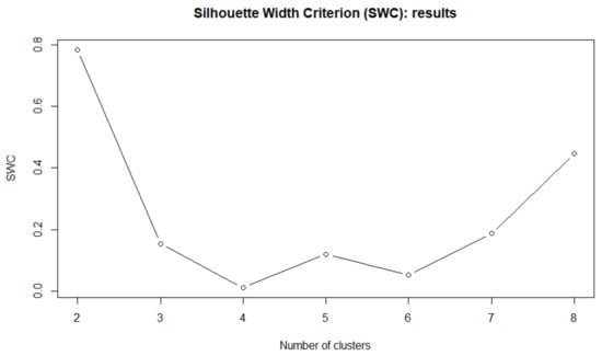
Figure 10.
SWC for the first 5-year observations (distribution-based clustering)—FTSE100 data.
On the other hand, following the same approach, the correlation-based clustering approach suggests the presence of clusters (see Figure 11) and an average silhouette equal to 0.08, 10 times lower than the one shown in Figure 10.
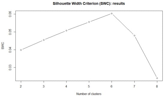
Figure 11.
SWC for the first 5-year observations (correlation-based clustering)—FTSE100 data.
In other words, on the basis of some in-sample arguments we can argue that the clustering resulting from the application of a distribution-based approach is much more accurate than another one based on correlation. The clusters composition for both approaches is shown in Table 8.
Table 8.
Final group assignment of the two alternative clustering approaches. The first column shows the results of the distribution-based approach, while the second column shows those of the correlation-based clustering (FTSE100 data).
Nevertheless, in this section we are interested in the out-of-sample performances in terms of portfolio selection. In the case of the distribution-based clustering, following [3], we consider the two clusters as two possible different portfolios. As stated before, we consider two alternative diversification rules, the naive () and the global minimum variance (GMV). Therefore, we have four possible trading strategies.
In the case of the correlation-based clustering, from Table 8 it clearly appears that the stocks AUTO, SVT, III, and FERG from single clusters. Therefore, we exclude these stocks and consider the clusters 1 and 3 as alternative portfolios, constructed with both naive and GMV diversification rules.
We compare the resulting portfolio in terms of return-risk trade-off represented by the Sharpe ratio, the amount of risk in worst scenarios computed by means of the value at risk (VaR) and the expected shortfall (ES) and the trading expenses through the turnover. The results are shown in Table 9.
Table 9.
Portfolio performance measures—experiment with FTSE100 data.
In general, following a naive diversification approach, all the portfolios built with the distribution-based clustering approach show much superior performances than those constructed with the alternative approach. Indeed, the two SEPD-based portfolios have a Sharpe ratio equal to 26.2% and 12.9%, respectively, while the alternative portfolios have lower Sharpe ratios equal to 21.6% and 2%.
In terms of VaR and expected shortfall the two SEPD-based portfolios built under naive diversification rule show similar risk profiles, with respect, the cluster 1 portfolio built through the correlation-based clustering, while the cluster 2 portfolio (correlation-based) has very high values compared to the others. Therefore, the SEPD-based clustered portfolios show a better return-risk profile, also in adverse scenarios.
In the end, since the weights’ structure do not change over time, the turnover of any naive portfolio is set to be zero.
On the side of the GMV diversification rules, the benefit of the distribution-based clustered portfolios are still evident. Indeed, although the best portfolio in terms of Sharpe ratio is the first cluster obtained by the correlation-based approach (SR equal to 29%), the portfolio built with the cluster 3 (correlation-based) shows a very poor Sharpe ratio performance equal to 5%.
The GMV portfolio built on the cluster 1 (SEPD-based) has a Sharpe ratio equal to 27.8%, while the one built on the cluster 2 has a Sharpe ratio of 12.3%. Clearly, once the cluster analysis is conducted, the investors do not know which portfolio will perform better in an out-of-sample. Therefore, let us suppose that ex ante we invest equally across the two clustered portfolios. The overall return of this investment strategy is higher if the investor chooses to invest in the SEPD-based clustered portfolios than in the case of correlation-based.
In terms of VaR and expected shortfall the results are even better. Indeed, in both the cases the two portfolios with the lowest VaR and ES are the SEPD-based clustered portfolios.
In terms of turnover, the SEPD-based cluster 2 shows the lowest value among the alternative and in general the SEPD-based trading rules have a much lower cost in aggregate.
Therefore, we can conclude that the SEPD-based entropy weighted algorithm proposed in Section 2, that aims to cluster stocks according to their distribution, shows good performances from a portfolio selection perspective. The correlation-based algorithm, that discard data distribution instead of correlations, performs poorer.
4.2. S&P500 Industrials
In this sub-section we provide the portfolio analysis for the second experiment with S&P500 Industrial real data. Nevertheless, in this case an important preliminary step to facilitate the analysis under consideration is to exclude from the sample the S&P500 industrial stocks showing missing values. Hence. from an initial sample of , we obtain a thinner sample of stocks.
As previously, we compare the distribution-based clustering approach presented in Section 2 with the correlation-based clustering, commonly used to form a portfolio of stocks. Figure 12 shows the SWC criterion according to different number of clusters C.
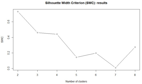
Figure 12.
SWC for the first 5-year observations (distribution-based clustering)—S&P500 data.
With a SWC greater than 0.8 we select . In Figure 13 is reported the same criterion in the case of the correlation-based clustering algorithm.
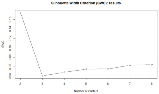
Figure 13.
SWC for the first 5-year observations (correlation-based clustering)—S&P500 data.
In this second experiment, the correlation-based clustering model suggests the same groups as the distribution-based one. However, the silhouette is again very low compared to the one shown in Figure 12, meaning that the quality of the resulting classification is much lower. The different clustering results are reported in Table 10.
Table 10.
Final group assignment of the two alternative clustering approaches. The first column shows the results of the distribution-based approach, while the second column shows those of the correlation-based clustering (S&P500 data).
The portfolio performances of the proposed approaches, assuming both naive and GMV diversification rules, are reported in the Table 11.
Table 11.
Portfolio performance measures—experiment with S&P500 data.
In the case of naive diversification rule, Table 11 shows that the best portfolio in terms of out-of-sample Sharpe ratio is the one based on cluster 1 resulting from the distribution-based clustering approach, with a value of 20%. Moreover, in terms of VaR and ES the two distribution-based clustered portfolios share similar risk than the correlation-based cluster 2 portfolio, while the correlation-based cluster 1 portfolio shows much higher values being, therefore, much more risky in adverse scenarios.
The construction of GMV portfolios, starting from the identified clusters, shows similarly interesting results. In particular, the distribution-based cluster 1 portfolio is still the highest performing, with a Sharpe ratio of 30%, while the correlation-based GMV cluster 1 portfolio has a performance lower than 20%. On the other side, both portfolios constructed on cluster 2 show similar Shape ratio but still the distribution-based allows a little over-performance of 10 basis points.
In terms of risk, looking at the VaR and ES, the distribution-based cluster 1 portfolio has a much lower amount of risk compared to the correlation-based cluster 1 portfolio and, at the same time, has a much higher Sharpe ratio. The other two portfolios constructed according to the the cluster 2 are again very similar.
In the end, we compare the portfolio performances with respect the turnover. The distribution-based cluster 2 portfolio has the lower turnover, while the correlation-based cluster 1 the highest. Moreover, the distribution-based cluster 1 portfolio has a more similar turnover than the correlation-based cluster 2, but with a Sharpe ratio higher than 11%.
Therefore, in this case we can conclude that the SEPD-based entropy weighted K-means approach developed in Section 2 allows the construction of high performance clustered portfolios, regardless the diversification rule used for their construction.
5. Conclusions
In this paper, we propose a new model-based clustering approach for classifying skewed and heavy tailed time series, by means of an entropy weighting clustering algorithm.
Clustering techniques are useful tools for exploratory data analysis in the way they identify common structures in an unlabeled dataset.
For example, a possible application of financial time series clustering concerns the asset allocation, where groups of similar stocks could be seen as portfolios of asset that shares similar characteristics.
Many recent papers aim to improve the existing clustering techniques for time series data. This article proposes a model clustering model that refers to data based on a very important family of asymmetric functions: the skewed exponential power distribution (SEPD), also known in literature as the skewed generalized error distribution (SGED). This distribution is very useful for classifying time series in the presence of fat-tailed and asymmetric time series.
The clustering algorithm, which represents the innovative aspect of this paper, applies the idea of entropy weighting clustering of [7,45] to the parameters estimated by a flexible probability distribution as in [23].
The criterion is that time series with similar parameter estimates are placed in the same group. Therefore, with a k-means clustering algorithm, the measure of dissimilarity is determined on the basis of these estimates. In this paper we, therefore, propose to combine all the information in an optimal way to form clusters.
Finally, to demonstrate the effectiveness of the proposed clustering approach, in this paper we propose two different applications to stock market data. Financial market data lend themselves well to adhering to our methodological proposal. In fact, the empirical densities of daily stock returns time series are proved to be non-Gaussian, asymmetric, and heavy.
Ours wants to be a fairly innovative research address and certainly many can be there financial applications that benefit from modeling equity returns via exponential power distribution and its extensions for skewness.
Indeed a final important result allows us to conclude that the new clustering algorithm we described in the paper can be used to form equity portfolios. Indeed, we compared the performances of the distribution-based clustering model proposed in this paper with a correlation-based clustering algorithm that is commonly used by financial practitioners to form portfolio of stocks. According to several measures, such as the Sharpe ratio, the value at risk, the expected shortfall, and the turnover we demonstrated the superior performances of the proposed clustering approach also from an asset allocation perspective.
A first possible future research can be devoted to the application of the proposed underlying idea to different probability distributions. For example, the asymmetric power distribution of [40] represents an interesting possibility for modeling situations where we suppose two different behaviors in the distribution’s tails.
Moreover, another interesting research direction can be devoted to the developments of a new distribution-based clustering approach where also the time varying parameters estimated from the skewed exponential power distribution (or others) are considered.
Author Contributions
Conceptualization, R.M., M.G. and K.G.; methodology, R.M., M.G. and K.G.; software, R.M., M.G. and K.G.; validation, R.M., M.G. and K.G.; formal analysis, R.M., M.G. and K.G.; investigation, R.M., M.G. and K.G.; resources, R.M., M.G. and K.G.; data curation, R.M., M.G. and K.G.; writing—original draft preparation, R.M., M.G. and K.G.; writing—review and editing, R.M., M.G. and K.G.; visualization, R.M., M.G. and K.G.; supervision, R.M., M.G. and K.G. All authors have read and agreed to the published version of the manuscript.
Funding
This research received no external funding.
Institutional Review Board Statement
Not applicable.
Informed Consent Statement
Not applicable.
Data Availability Statement
Data can be retrieved at the following link: https://www.sites.google.com/view/raffaele-mattera/research, accessed on 25 May 2021.
Conflicts of Interest
The authors declare no conflict of interest.
Appendix A. List of Stocks
Table A1.
List of stocks (FTSE100) considered in the application with real data.
Table A1.
List of stocks (FTSE100) considered in the application with real data.
| ID | Name | Symbol | Sector |
|---|---|---|---|
| 1 | 3i | III | Financial Services |
| 2 | Admiral Group | ADM | Nonlife Insurance |
| 3 | Anglo American plc | AAL | Mining |
| 5 | Ashtead Group | AHT | Support Services |
| 7 | AstraZeneca | AZN | Pharmaceuticals and Biotechnology |
| 8 | Auto Trader Group | AUTO | Media |
| 12 | B&M | BME | Retailers |
| 13 | BAE Systems | BA. | Aerospace and Defence |
| 17 | BHP | BHP | Mining |
| 25 | Compass Group | CPG | Support Services |
| 26 | CRH plc | CRH | Construction and Materials |
| 29 | Diageo | DGE | Beverages |
| 31 | Evraz | EVR | Industrial Metals and Mining |
| 33 | Ferguson plc | FERG | Support Services |
| 36 | GlaxoSmithKline | GSK | Pharmaceuticals and Biotechnology |
| 42 | IHG Hotels & Resorts | IHG | Travel and Leisure |
| 46 | International Airlines Group | IAG | Travel and Leisure |
| 56 | M&G | MNG | Asset Managers |
| 57 | Melrose Industries | MRO | Automobiles and Parts |
| 60 | NatWest Group | NWG | Banks |
| 68 | Prudential plc | PRU | Life Insurance |
| 74 | Rio Tinto | RIO | Mining |
| 83 | Severn Trent | SVT | Gas, Water, and Multi-utilities |
| 94 | Tesco | TSCO | Food & Drug Retailers |
| 97 | Vodafone Group | VOD | Mobile Telecommunications |
| 100 | WPP plc | WPP | Media |
Table A2.
List of stocks (FTSE100) considered in the application with real data.
Table A2.
List of stocks (FTSE100) considered in the application with real data.
| ID | Symbol | Name |
|---|---|---|
| 1 | MMM | 3M Company |
| 2 | AOS | A.O. Smith Corp |
| 16 | ALK | Alaska Air Group |
| 21 | ALLE | Allegion |
| 30 | AAL | American Airlines Group |
| 38 | AME | Ametek |
| 70 | BA | Boeing Company |
| 79 | CHRW | C. H. Robinson Worldwide |
| 88 | CARR | Carrier Global |
| 90 | CAT | Caterpillar Inc. |
| 107 | CTAS | Cintas Corporation |
| 123 | CPRT | Copart Inc |
| 128 | CSX | CSX Corp. |
| 129 | CMI | Cummins Inc. |
| 135 | DE | Deere and Co. |
| 136 | DAL | Delta Air Lines Inc. |
| 150 | DOV | Dover Corporation |
| 158 | ETN | Eaton Corporation |
| 164 | EMR | Emerson Electric Company |
| 168 | EFX | Equifax Inc. |
| 179 | EXPD | Expeditors |
| 184 | FAST | Fastenal Co |
| 186 | FDX | FedEx Corporation |
| 197 | FTV | Fortive Corp |
| 198 | FBHS | Fortune Brands Home & Security |
| 206 | GNRC | Generac Holdings |
| 207 | GD | General Dynamics |
| 208 | GE | General Electric |
| 216 | GWW | Grainger (W.W.) Inc. |
| 230 | HON | Honeywell Int’l Inc. |
| 233 | HWM | Howmet Aerospace |
| 237 | HII | Huntington Ingalls Industries |
| 238 | IEX | IDEX Corporation |
| 240 | INFO | IHS Markit |
| 241 | ITW | Illinois Tool Works |
| 244 | IR | Ingersoll-Rand |
| 257 | JBHT | J. B. Hunt Transport Services |
| 259 | J | Jacobs Engineering Group |
| 262 | JCI | Johnson Controls International |
| 265 | KSU | Kansas City Southern |
| 276 | LHX | L3Harris Technologies |
| 282 | LDOS | Leidos Holdings |
| 289 | LMT | Lockheed Martin Corp. |
| 301 | MAS | Masco Corp. |
| 333 | NLSN | Nielsen Holdings |
| 336 | NSC | Norfolk Southern Corp. |
| 338 | NOC | Northrop Grumman |
| 349 | ODFL | Old Dominion Freight Line |
| 353 | OTIS | Otis Worldwide |
| 354 | PCAR | Paccar |
| 356 | PH | Parker-Hannifin |
| 361 | PNR | Pentair plc |
| 387 | PWR | Quanta Services Inc. |
| 391 | RTX | Raytheon Technologies |
| 396 | RSG | Republic Services Inc. |
| 398 | RHI | Robert Half International |
| 399 | ROK | Rockwell Automation Inc. |
| 400 | ROL | Rollins Inc. |
| 401 | ROP | Roper Technologies |
| 415 | SNA | Snap-on |
| 417 | LUV | Southwest Airlines |
| 418 | SWK | Stanley Black and Decker |
| 433 | TDY | Teledyne Technologies |
| 438 | TXT | Textron Inc. |
| 449 | TT | Trane Technologies plc |
| 450 | TDG | TransDigm Group |
| 461 | UNP | Union Pacific Corp. |
| 462 | UAL | United Airlines Holdings |
| 463 | UPS | United Parcel Service |
| 464 | URI | United Rentals Inc. |
| 471 | VRSK | Verisk Analytics |
| 483 | WM | Waste Management Inc. |
| 491 | WAB | Westinghouse Air Brake Technologies Corp. |
| 500 | XYL | Xylem Inc. |
References
- Mantegna, R.N. Hierarchical structure in financial markets. Eur. Phys. J. B-Condens. Matter Complex Syst. 1999, 11, 193–197. [Google Scholar] [CrossRef]
- Tola, V.; Lillo, F.; Gallegati, M.; Mantegna, R.N. Cluster analysis for portfolio optimization. J. Econ. Dyn. Control 2008, 32, 235–258. [Google Scholar] [CrossRef]
- Iorio, C.; Frasso, G.; D’Ambrosio, A.; Siciliano, R. A P-spline based clustering approach for portfolio selection. Expert Syst. Appl. 2018, 95, 88–103. [Google Scholar] [CrossRef]
- Liao, T.W. Clustering of time series data—A survey. Pattern Recognit. 2005, 38, 1857–1874. [Google Scholar] [CrossRef]
- D’Urso, P. Dissimilarity measures for time trajectories. Stat. Methods Appl. 2000, 1, 53–83. [Google Scholar] [CrossRef]
- D’Urso, P. Fuzzy C-means clustering models for multivariate time-varying data: Different approaches. Int. J. Uncertain. Fuzziness Knowl. Based Syst. 2004, 12, 287–326. [Google Scholar] [CrossRef]
- Coppi, R.; D’Urso, P. Fuzzy unsupervised classification of multivariate time trajectories with the Shannon entropy regularization. Comput. Stat. Data Anal. 2006, 50, 1452–1477. [Google Scholar] [CrossRef]
- Coppi, R.; D’Urso, P.; Giordani, P. A fuzzy clustering model for multivariate spatial time series. J. Classif. 2010, 27, 54–88. [Google Scholar] [CrossRef]
- D’Urso, P.; De Giovanni, L.; Massari, R. Robust fuzzy clustering of multivariate time trajectories. Int. J. Approx. Reason. 2018, 99, 12–38. [Google Scholar] [CrossRef]
- Caiado, J.; Crato, N.; Peña, D. Comparison of times series with unequal length in the frequency domain. Commun. Stat. Simul. Comput. 2009, 38, 527–540. [Google Scholar] [CrossRef]
- Alonso, A.M.; Maharaj, E.A. Comparison of time series using subsampling. Comput. Stat. Data Anal. 2006, 50, 2589–2599. [Google Scholar] [CrossRef]
- D’Urso, P.; Maharaj, E.A. Autocorrelation-based fuzzy clustering of time series. Fuzzy Sets Syst. 2009, 160, 3565–3589. [Google Scholar] [CrossRef]
- Caiado, J.; Crato, N.; Peña, D. A periodogram-based metric for time series classification. Comput. Stat. Data Anal. 2006, 50, 2668–2684. [Google Scholar] [CrossRef]
- D’Urso, P.; Maharaj, E.A. Wavelets-based clustering of multivariate time series. Fuzzy Sets Syst. 2012, 193, 33–61. [Google Scholar] [CrossRef]
- Maharaj, E.A.; D’Urso, P.; Galagedera, D.U. Wavelet-based fuzzy clustering of time series. J. Classif. 2010, 27, 231–275. [Google Scholar] [CrossRef]
- Maharaj, E.A.; D’Urso, P. Fuzzy clustering of time series in the frequency domain. Inf. Sci. 2011, 181, 1187–1211. [Google Scholar] [CrossRef]
- D’Urso, P.; De Giovanni, L.; Massari, R.; D’Ecclesia, R.L.; Maharaj, E.A. Cepstral-based clustering of financial time series. Expert Syst. Appl. 2020, 161, 113705. [Google Scholar] [CrossRef]
- Piccolo, D. A distance measure for classifying ARIMA models. J. Time Ser. Anal. 1990, 11, 153–164. [Google Scholar] [CrossRef]
- Otranto, E. Clustering heteroskedastic time series by model-based procedures. Comput. Stat. Data Anal. 2008, 52, 4685–4698. [Google Scholar] [CrossRef]
- D’Urso, P.; De Giovanni, L.; Massari, R. GARCH-based robust clustering of time series. Fuzzy Sets Syst. 2016, 305, 1–28. [Google Scholar] [CrossRef]
- Iorio, C.; Frasso, G.; D’Ambrosio, A.; Siciliano, R. Parsimonious time series clustering using p-splines. Expert Syst. Appl. 2016, 52, 26–38. [Google Scholar] [CrossRef]
- Maharaj, E.A.; Alonso, A.M.; D’Urso, P. Clustering seasonal time series using extreme value analysis: An application to Spanish temperature time series. Commun. Stat. Case Stud. Data Anal. Appl. 2015, 1, 175–191. [Google Scholar] [CrossRef]
- D’Urso, P.; Maharaj, E.A.; Alonso, A.M. Fuzzy clustering of time series using extremes. Fuzzy Sets Syst. 2017, 318, 56–79. [Google Scholar] [CrossRef]
- Corduas, M.; Piccolo, D. Time series clustering and classification by the autoregressive metric. Comput. Stat. Data Anal. 2008, 52, 1860–1872. [Google Scholar] [CrossRef]
- D’Urso, P.; Cappelli, C.; Di Lallo, D.; Massari, R. Clustering of financial time series. Phys. A Stat. Mech. Its Appl. 2013, 392, 2114–2129. [Google Scholar] [CrossRef]
- Cerqueti, R.; Giacalone, M.; Mattera, R. Model-based fuzzy time series clustering of conditional higher moments. Int. J. Approx. Reason. 2021, 134, 34–52. [Google Scholar] [CrossRef]
- Fernandez, C.; Osiewalski, J.; Steel, M.F. Modeling and inference with υ-spherical distributions. J. Am. Stat. Assoc. 1995, 90, 1331–1340. [Google Scholar] [CrossRef]
- Fernández, C.; Steel, M.F. On Bayesian modeling of fat tails and skewness. J. Am. Stat. Assoc. 1998, 93, 359–371. [Google Scholar]
- Theodossiou, P. Skewed generalized error distribution of financial assets and option pricing. Multinatl. Financ. J. 2015, 19, 223–266. [Google Scholar] [CrossRef]
- Komunjer, I. Asymmetric power distribution: Theory and applications to risk measurement. J. Appl. Econom. 2007, 22, 891–921. [Google Scholar] [CrossRef]
- Hsieh, D.A. Modeling heteroscedasticity in daily foreign-exchange rates. J. Bus. Econ. Stat. 1989, 7, 307–317. [Google Scholar]
- Nelson, D.B. Conditional heteroskedasticity in asset returns: A new approach. Econom. J. Econom. Soc. 1991, 59, 347–370. [Google Scholar] [CrossRef]
- Duan, J.C. Conditionally Fat-Tailed Distributions and the Volatility Smile in Options; Working Paper; Rotman School of Management, University of Toronto: Toronto, ON, Canada, 1999. [Google Scholar]
- Ayebo, A.; Kozubowski, T.J. An asymmetric generalization of Gaussian and Laplace laws. J. Probab. Stat. Sci. 2003, 1, 187–210. [Google Scholar]
- Christoffersen, P.; Dorion, C.; Jacobs, K.; Wang, Y. Volatility components, affine restrictions, and nonnormal innovations. J. Bus. Econ. Stat. 2010, 28, 483–502. [Google Scholar] [CrossRef]
- Mattera, R.; Giacalone, M. Alternative distribution based GARCH models for bitcoin volatility estimation. Empir. Econ. Lett. 2018, 17, 1283–1288. [Google Scholar]
- Cerqueti, R.; Giacalone, M.; Panarello, D. A Generalized Error Distribution Copula-based method for portfolios risk assessment. Phys. A Stat. Mech. Its Appl. 2019, 524, 687–695. [Google Scholar] [CrossRef]
- Cerqueti, R.; Giacalone, M.; Mattera, R. Skewed non-Gaussian GARCH models for cryptocurrencies volatility modelling. Inf. Sci. 2020, 527, 1–26. [Google Scholar] [CrossRef]
- Trucíos, C. Forecasting Bitcoin risk measures: A robust approach. Int. J. Forecast. 2019, 35, 836–847. [Google Scholar] [CrossRef]
- Zhu, D.; Zinde-Walsh, V. Properties and estimation of asymmetric exponential power distribution. J. Econom. 2009, 148, 86–99. [Google Scholar] [CrossRef]
- Kotz, S.; Kozubowski, T.; Podgorski, K. The Laplace Distribution and Generalizations: A Revisit with Applications to Communications, Economics, Engineering, and Finance; Springer Science & Business Media: Berlin/Heidelberg, Germany, 2012. [Google Scholar]
- Giacalone, M.; Panarello, D.; Mattera, R. Multicollinearity in regression: An efficiency comparison between Lp-norm and least squares estimators. Qual. Quant. 2018, 52, 1831–1859. [Google Scholar] [CrossRef]
- Giacalone, M. A combined method based on kurtosis indexes for estimating p in non-linear Lp-norm regression. Sustain. Futur. 2020, 2, 100008. [Google Scholar] [CrossRef]
- Mudholkar, G.S.; Hutson, A.D. The epsilon–skew–normal distribution for analyzing near-normal data. J. Stat. Plan. Inference 2000, 83, 291–309. [Google Scholar] [CrossRef]
- Jing, L.; Ng, M.K.; Huang, J.Z. An entropy weighting k-means algorithm for subspace clustering of high-dimensional sparse data. IEEE Trans. Knowl. Data Eng. 2007, 19, 1026–1041. [Google Scholar] [CrossRef]
- Huang, J.Z.; Ng, M.K.; Rong, H.; Li, Z. Automated variable weighting in k-means type clustering. IEEE Trans. Pattern Anal. Mach. Intell. 2005, 27, 657–668. [Google Scholar] [CrossRef]
- Eshima, N. Statistical Data Analysis and Entropy; Springer: Berlin/Heidelberg, Germany, 2020. [Google Scholar]
- Rousseeuw, P.J. Silhouettes: A graphical aid to the interpretation and validation of cluster analysis. J. Comput. Appl. Math. 1987, 20, 53–65. [Google Scholar] [CrossRef]
- Adcock, C.; Eling, M.; Loperfido, N. Skewed distributions in finance and actuarial science: A review. Eur. J. Financ. 2015, 21, 1253–1281. [Google Scholar] [CrossRef]
- Cont, R. Empirical properties of asset returns: Stylized facts and statistical issues. Quant. Financ. 2001, 1, 223–236. [Google Scholar] [CrossRef]
- Jarque, C.M.; Bera, A.K. A test for normality of observations and regression residuals. Int. Stat. Rev. Int. Stat. 1987, 55, 163–172. [Google Scholar] [CrossRef]
- Bodnar, T.; Mazur, S.; Okhrin, Y. Bayesian estimation of the global minimum variance portfolio. Eur. J. Oper. Res. 2017, 256, 292–307. [Google Scholar] [CrossRef]
- Bodnar, T.; Gupta, A.K. Robustness of the inference procedures for the global minimum variance portfolio weights in a skew-normal model. Eur. J. Financ. 2015, 21, 1176–1194. [Google Scholar] [CrossRef]
- Bodnar, T.; Mazur, S.; Podgórski, K. A test for the global minimum variance portfolio for small sample and singular covariance. AStA Adv. Stat. Anal. 2017, 101, 253–265. [Google Scholar] [CrossRef]
- Pappas, D.; Kiriakopoulos, K.; Kaimakamis, G. Optimal portfolio selection with singular covariance matrix. Int. Math. Forum 2010, 5, 2305–2318. [Google Scholar]
- Bodnar, T.; Mazur, S.; Podgórski, K. Singular inverse Wishart distribution and its application to portfolio theory. J. Multivar. Anal. 2016, 143, 314–326. [Google Scholar] [CrossRef]
- Bodnar, T.; Mazur, S.; Podgórski, K.; Tyrcha, J. Tangency portfolio weights for singular covariance matrix in small and large dimensions: Estimation and test theory. J. Stat. Plan. Inference 2019, 201, 40–57. [Google Scholar] [CrossRef]
- Gulliksson, M.; Mazur, S. An iterative approach to ill-conditioned optimal portfolio selection. Comput. Econ. 2019, 56, 773–794. [Google Scholar] [CrossRef]
- De Miguel, V.; Garlappi, L.; Uppal, R. Optimal versus naive diversification: How inefficient is the 1/N portfolio strategy? Rev. Financ. Stud. 2007, 22, 1915–1953. [Google Scholar] [CrossRef]
Publisher’s Note: MDPI stays neutral with regard to jurisdictional claims in published maps and institutional affiliations. |
© 2021 by the authors. Licensee MDPI, Basel, Switzerland. This article is an open access article distributed under the terms and conditions of the Creative Commons Attribution (CC BY) license (https://creativecommons.org/licenses/by/4.0/).