Fractional Order Models Are Doubly Infinite Dimensional Models and thus of Infinite Memory: Consequences on Initialization and Some Solutions

Abstract

Using a small number of mathematical transformations, this article examines the nature of fractional models described by fractional differential equations or pseudo state space descriptions. Computation of the impulse response of a fractional model using the Cauchy method shows that they exhibit infinitely small and high time constants. This impulse response can be rewritten as a diffusive representation whose Fourier transform permits a representation of a fractional model by a diffusion equation in an infinite space domain. Fractional models can thus be viewed as doubly infinite dimensional models: infinite as distributed with a distribution in an infinite domain. This infinite domain or the infinitely large time constants of the impulse response reveal a property intrinsic to fractional models: their infinite memory. Solutions to generate fractional behaviors without infinite memory are finally proposed.

1. Introduction

A confusion or rather an implicit link exists between fractional behaviors (of physical, biological, thermal, etc., origin) and fractional models (a tool to model fractional behaviors) [1]. To deliberately limit this confusion, the name “fractional behavior” is replaced by “power-law behaviors”, which well expresses the idea that studied behaviors exhibit, in a limited frequency or time domain, a power-law-type response.

It is now evident that power-law behaviors are ubiquitous in numerous domains and that appropriate modelling tools are needed. Due to the dynamic behavior similarity between power-law behaviors and fractional models, the latter have therefore naturally been used as modelling tools.

The field of fractional calculus research has thus undergone numerous (although perhaps not fundamental) developments [2] and many applications of fractional order derivatives now exist [3]. Fractional calculus has become a common modeling tool in many fields [4,5,6,7].

However, this link between power-law behaviors and fractional models often found in the literature does not result from physical justification, as noted in the present paper. Many researchers have nevertheless contributed to the study of fractional calculus and fractional models, sometimes yielding to the ease of generalizing the results dedicated to classical integer systems (which are sometimes referred to as “fractionalizations”).

However, it is also well known that fractional models have several drawbacks [8,9,10]. The most important of these, from which some others derive, is they were not deduced from physical considerations but are only generalizations of existing (integer) tools. Consequently, fractional models are imbued with an intrinsic and unrealistic property: they are doubly infinite dimensional models:

-

infinite as they are distributed

-

and infinite as they are defined (the parameter distribution) in an infinite spatial domain.

It is only by trying to analyze the physical meaning of fractional models that this property is revealed.

Giving meaning to fractional models (a posteriori) has nevertheless been a concern of many researchers. Mathematical [11,12], physical [13,14], geometrical [15,16], and statistical [17] meanings were therefore sought but these approaches do not help to understand their nature and, in particular, their advantages and disadvantages. It was even attempted to deduce a model from a physical phenomenon [18,19] but infinite spatial dimensions were considered in order to do so, which tends on the contrary to demonstrate the physical inconsistency of a fractional model.

The infinite spatial dimension is the conclusion also reached in this work after some mathematical transformations that lead to a representation of a fractional model by a diffusion equation. This representation is obtained through the Fourier transform of the diffusive representation of a fractional model. It is also shown that the diffusive representation can be deduced from the impulse response of a fractional model computed using the Cauchy method. The diffusive representation obtained exhibits infinitely large time constants that are a consequence of the definition of fractional models in an infinite spatial domain. This infinite dimension or these infinitely large time constants are responsible for the infinite memory of fractional models. All these concepts are detailed and demonstrated in this paper. Finally, a list of alternative solutions to fractional models to produce power-law behaviors is given.

2. A physical and Systemic Analysis of Fractional Models

2.1. Model Definition

Although the terms used to designate them are very similar, power-law behavior and fractional models are two different concepts. Power-law (dynamical) behavior qualifies the nature of some real systems that exhibit a power law behavior in a limited time or frequency band (the system impulse response behaves as $t^{-\nu }$ in a given time band or the system frequency response behaves as ${\left(j\omega \right)}^{-1+\nu }$ in a given frequency band). Fractional models are a class of models that was introduced to capture power-law behaviors. Without considering physical justifications, fractional models were introduced by simply generalizing existing modelling tools, by simply replacing the classical differentiation operators by fractional differentiation operators. These fractional derivation operators had long been mathematically defined and were in fact known to exhibit power-law behaviors (but not only over a limited time or frequency band). For this reason, fractional differential equations appeared as possible models to capture some power-law behaviors.

With $u\left(t\right)\in ℝ$ and $y\left(t\right)\in ℝ$ respectively as input and output, a fractional differential equation is found in the literature with the form:

$${\displaystyle \sum }_{k=0}^{N_a}{a}_k{\mathit{D}}_{t_0}^{{\nu }_{a_k}}\left(y\left(t\right)\right)={\displaystyle \sum }_{k=0}^{N_b}{b}_k{\mathit{D}}_{t_0}^{{\nu }_{b_k}}\left(u\left(t\right)\right)$$

(1)

In Relation (1) $a_k\in ℝ$ and $b_k\in ℝ$. ${\mathit{D}}_{t_0}^{{\nu }_{a_k}}$ and ${\mathit{D}}_{t_0}^{{\nu }_{b_k}}$ denote, respectively, fractional differentiation operators of orders ${\nu }_{a_k}\in ℝ$ and ${\nu }_{b_k}\in ℝ$ [20]. Various definitions can be used to describe these operators [21], which raises the question of choice. These definitions are in certain respects equivalent, but differences exist, notably regarding how initial conditions are taken into account.

The “fractionalization” of another well-known modelling tool was also proposed in the literature if the differentiation orders ${\nu }_{a_k}$ and ${\nu }_{b_k}$ met the following conditions:

$${\nu }_{a_k}=\frac{k}{q},{\nu }_{b_k}=\frac{k}{q}, q\in {\mathbb{N}}^{*}$$

(2)

These conditions, known as commensurability conditions, enable Relation (1) to be rewritten as (under null initial conditions):

$$\{\begin{array}{c}{\mathit{D}}_{t_0}^{\nu }X\left(t\right)=AX\left(t\right)+Bu\left(t\right)\\ y\left(t\right)=CX\left(t\right)+\mathit{D}u\left(t\right)\end{array}$$

(3)

This representation is known in the literature as a pseudo state space description. “Pseudo” because the vector $X\left(t\right)\in {ℝ}^n$ cannot be viewed as the model state since this is not the minimal amount of information required to predict the future of the model. In Relation (3), $\nu =1/q$ is the fractional order of the model and $A\in {ℝ}^{n\times n}$, $B\in {ℝ}^{n\times 1}$, $C\in {ℝ}^{1\times n}$, and $D\in ℝ$ are constant matrices.

Application of the Laplace transform to Relations (1) or (3) (with null initial conditions) permits a transfer function representation of the form:

$$H\left(s\right)=\frac{Y\left(s\right)}{U\left(s\right)}=\frac{\mathcal{L}\left\{y\left(t\right)\right\}}{\mathcal{L}\left\{u\left(t\right)\right\}}$$

(4)

Models (1) and (3) are very widely used in the literature when talking about fractional models.

Example 1.

The following fractional model, which will be used repeatedly throughout the article, is now considered:

$${\mathit{D}}_0^{1.8}y\left(t\right)+y\left(t\right)=8{\mathit{D}}_0^{1.2}u\left(t\right)-8{\mathit{D}}_0^{0.6}u\left(t\right)+10u\left(t\right)$$

(5)

As all the fractional orders are multiples of 0.6, such a model admits the following pseudo state space description:

$$\{\begin{array}{c}{\mathit{D}}_0^{0.6}X\left(t\right)=AX\left(t\right)+Bu\left(t\right)\\ y\left(t\right)=CX\left(t\right)\end{array}$$

(6)

with

$$X\left(t\right)=\left[\begin{array}{c}x\left(t\right)\\ {\mathit{D}}_0^{0.6}x\left(t\right)\\ {\mathit{D}}_0^{1.2}x\left(t\right)\end{array}\right]A=\left[\begin{array}{ccc}0& 1& 0\\ 0& 0& 1\\ -1& 0& 0\end{array}\right]B=\left[\begin{array}{c}0\\ 0\\ 1\end{array}\right]C=\left[\begin{array}{ccc}10& -8& 8\end{array}\right].$$

(7)

This model transfer function is thus given by:

$$H\left(s\right)=\frac{8s^{1.2}-8s^{0.6}+10}{s^{1.8}+1}.$$

(8)

As previously mentioned, the definition of these models did not result from physical analyses; they are “fractionalizations” of classical models. The objective of the following sections is therefore to propose an analysis of the physical meaning of these models.

2.2. Poles and Time Constants Distribution and Infinite Memory

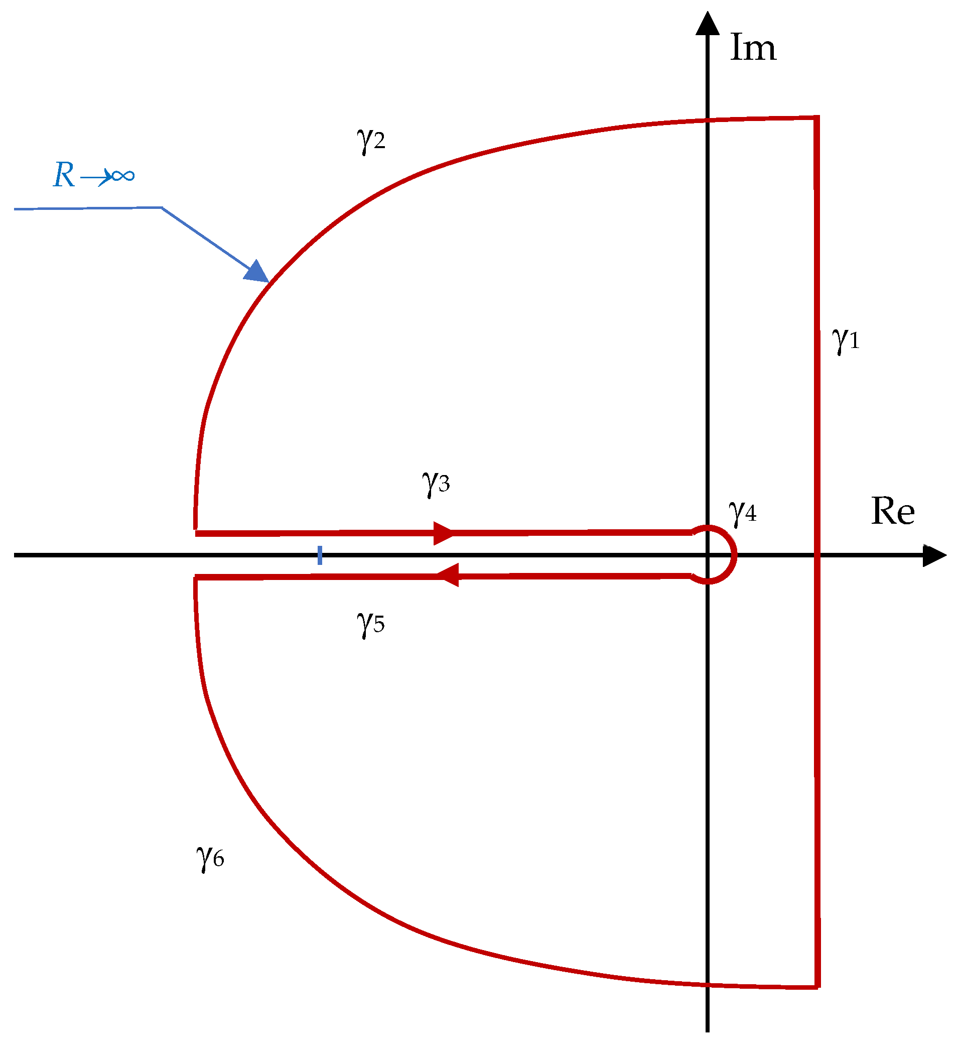
The first physical analysis proposed is based on the impulse response of the Models (1) and (3). This impulse response is given by the inverse Laplace transformation relation:

$$h\left(t\right)={\mathcal{L}}^{-1}\left\{H\left(s\right)\right\}=\frac{1}{2j\pi }{{\displaystyle \int }}_{c-j\infty }^{c+j\infty }H\left(s\right)e^{st}ds.$$

(9)

In Relation (9), the value of $c$ is chosen to be greater than the $H\left(s\right)$ singular point abscissa and the integral computation is performed on the Bromwich–Wagner path $\Gamma$ of Figure 1 that bypasses the negative axis around the branching point $z=0$ for $t>0$. It thus avoids the complex plane domain for which the transfer function $s^{\nu }=0$ is not defined, i.e., the segment [−∞, 0]. As shown by Figure 1, the path is the union of six sub-paths: $\Gamma ={\gamma }_1\cup \dots \cup {\gamma }_6$.

Using the residue theorem, Relation (9) can be rewritten as:

$$h\left(t\right)=-\frac{1}{2\pi j}\underset{\Gamma -{\gamma }_1}{{\displaystyle \int }}H\left(s\right)e^{ts}ds+{\displaystyle \sum }_{\begin{array}{c}poles\\ in \Gamma \end{array}}\mathrm{Res}\left[H\left(s\right)e^{ts}\right]$$

(10)

with, in the case of a simple pole $p$ for $H\left(s\right)e^{ts}$:

$$Re{s}_p\left[H\left(s\right)e^{ts}\right]=\underset{z\to p}{\lim }\left(z-p\right)H\left(z\right)e^{tz}.$$

(11)

Relation (10) thus imposes the computation of the poles of $H\left(s\right)$ and shows that the impulse responses of Models (1) and (3) can be split into two parts:

$$h\left(t\right)=h_p\left(t\right)+h_d\left(t\right).$$

(12)

The function $h_p\left(t\right)$ is computed from the poles of Models (1) and (3) (residues of the Cauchy method). The function $h_d\left(t\right)$ is linked to the diffusive part of the model. The name “diffusive” is explained in the sequel (see Section 2.3). The function $h_d\left(t\right)$ is defined by [22]:

$$h_d\left(t\right)={{\displaystyle \int }}_0^{\infty }\mu \left(z\right)e^{-tz}dz$$

(13)

in which the function $\mu \left(x\right)$ is given [23] by:

$$\mu \left(z\right)=\frac{1}{2i\pi }\left[H\left({\left(-z\right)}^{-}\right)-H\left({\left(-z\right)}^{+}\right)\right] \mathrm{with} \mu \left(z\right)\in ℝ.$$

(14)

The Laplace transform of function $h_d\left(t\right)$ is given by:

$$h_d\left(s\right)={{\displaystyle \int }}_0^{\infty }\frac{\mu \left(z\right)}{s+z}dz.$$

(15)

Example 2.

The model defined by Relation (5) is again considered. The corresponding transfer function (Relation (8)) can be rewritten as:

$$H\left(s\right)=\frac{2}{s^{1.8}+1}+\frac{8}{s^{0.6}+1}.$$

(16)

The poles of the model, denoted  $s_k={\rho }_k{e}^{j{\theta }_k}$, are the values of s such that  ${\theta }_k\in \left[-\pi ,\pi \right]$  and:

$$s_k{}^{1.8}+1=0 \mathrm{or} s_k{}^{0.6}+1=0$$

(17)

or:

$$s_k{}^{1.8}=e^{j\left(\pi +2k\pi \right)} \mathrm{or} s_k{}^{0.6}=e^{j\left(\pi +2k\pi \right)}$$

(18)

and thus:

$$s_k=e^{j\frac{\left(\pi +2k\pi \right)}{1.8}} \mathrm{or} s_k=e^{j\frac{\left(\pi +2k\pi \right)}{0.6}}$$

(19)

if there exist values of k such that:

$$\frac{\left(\pi +2k\pi \right)}{1.8}\in \left[-\pi ,\pi \right] \mathrm{or} \frac{\left(\pi +2k\pi \right)}{0.6}\in \left[-\pi ,\pi \right].$$

(20)

Two poles are produced by Relation (20):

$$s_0=e^{j\frac{\pi }{1.8}} \mathrm{or} s_1=e^{-j\frac{\pi }{1.8}}$$

(21)

that generate the function:

$$h_p\left(t\right)=2\left(e^{e^{j\frac{\pi }{1.8}t}}+e^{e^{-j\frac{\pi }{1.8}t}}\right)=4e^{cos\left(\frac{\pi }{1.8}\right)t}cos\left(sin\left(\frac{\pi }{1.8}\right)t\right).$$

(22)

According to Relations (13) and (14), the function$h_d\left(t\right)$ is given by:

$$h_d\left(t\right)={{\displaystyle \int }}_0^{\infty }\left(\frac{2sin\left(1.8\pi \right)}{\pi }\frac{z^{1.8}}{1-2z^{1.8}cos\left(1.8\pi \right)+z^{3.6}}+\frac{8sin\left(0.6\pi \right)}{\pi }\frac{z^{0.6}}{1-2z^{0.6}cos\left(0.6\pi \right)+z^{1.2}}\right)e^{-tz}dz$$

(23)

which corresponds to Relation (13) with:

$$\mu \left(z\right)=\frac{2sin\left(1.8\pi \right)}{\pi }\frac{z^{1.8}}{1-2z^{1.8}cos\left(1.8\pi \right)+z^{3.6}}+\frac{8sin\left(0.6\pi \right)}{\pi }\frac{z^{0.6}}{1-2z^{0.6}cos\left(0.6\pi \right)+z^{1.2}}$$

(24)

which is represented by Figure 2.

If an input $u\left(t\right)$ is applied to the diffusive part with an impulse response $h_d\left(t\right)$, the output $y_d\left(t\right)$ is the convolution product:

$$y_d\left(t\right)={{\displaystyle \int }}_0^{\mathrm{t}}{{\displaystyle \int }}_0^{\infty }\mu \left(z\right)e^{-\left(t-\tau \right)z}u\left(\tau \right)dzd\tau ={{\displaystyle \int }}_0^{\infty }\mu \left(z\right){{\displaystyle \int }}_0^{\mathrm{t}}{e}^{-\left(t-\tau \right)z}u\left(\tau \right)d\tau dz.$$

(25)

Introducing the function $w\left(t,z\right)$ such that:

$$w\left(t,z\right)={{\displaystyle \int }}_0^{\mathrm{t}}{e}^{-\left(t-\tau \right)z}u\left(\tau \right)d\tau .$$

(26)

Relation (25) can be rewritten as:

$$\{\begin{array}{l}\frac{\partial w\left(t,z\right)}{\partial t}=-zw\left(t,z\right)+u\left(t\right)\\ y_d\left(t\right)={{\displaystyle \int }}_0^{\infty }\mu \left(z\right)w\left(t,z\right)dz\end{array}z\in {ℝ}_{+}.$$

(27)

This representation is known in the literature as the diffusive representation [22,23].

Representations (15) and (27) of fractional models are particularly interesting because they make it possible to reveal properties that are poorly known and yet fundamental, because they provide information on the internal nature of fractional models and about how to initialize them. Relation (15) highlights that Models (1) and (3) have poles (values of $z$) distributed from 0 to $-\infty$. Models (1) and (3) are thus fitted with infinitely fast and infinitely slow time constants (they are attenuated by the function $\mu ( )$, but they exist). Relation (27) reveals the impact of these poles (or time constants) on the initialization of fractional models. All the poles must be initialized as the function $w\left(0,z\right)$ must be initialized with $z\in {ℝ}_{+}$. This provides fractional models with an infinite memory.

Note that a link between fractional operators and poles distribution from 0 to $-\infty$ was also highlighted in [24].

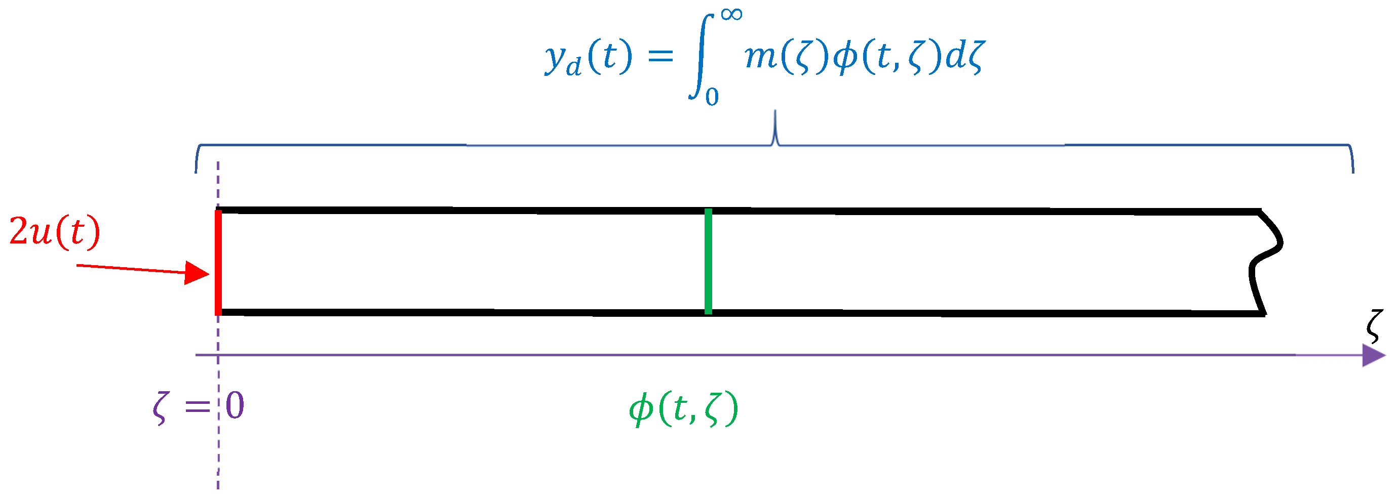
2.3. Spatial Definition and Infinite Memory

In this section, we try to obtain a spatial representation of fractional models. To this end, Model (27) is rewritten as:

$$\{\begin{array}{c}\frac{\partial w\left(t,z\right)}{\partial t}=-zw\left(t,z\right)+u\left(t\right)\\ y_d\left(t\right)=\frac{1}{2}{{\displaystyle \int }}_0^{\infty }\mu \left(z\right)w\left(t,z\right)dz+\frac{1}{2}{{\displaystyle \int }}_0^{\infty }\mu \left(z\right)w\left(t,z\right)dz\end{array}z\in {ℝ}_{+}.$$

(28)

The changes of variable $\rho =-\sqrt{z}$ and $\rho =\sqrt{z}$ are respectively used in the first and second integral of Relation (28). The resulting model is thus:

$$\{\begin{array}{c}\frac{\partial \psi \left(t,\rho \right)}{\partial t}=-{\rho }^2\psi \left(t,\rho \right)+u\left(t\right)\\ y_d\left(t\right)=\frac{1}{2}{{\displaystyle \int }}_0^{-\infty }2\rho \mu \left({\rho }^2\right)\psi \left(t,\rho \right)d\rho +\frac{1}{2}{{\displaystyle \int }}_0^{\infty }2\rho \mu \left({\rho }^2\right)\psi \left(t,\rho \right)d\rho \end{array}\rho \in ℝ$$

(29)

with $\psi \left(t,\rho \right)=w\left(t,{\rho }^2\right)$. After simplifications, Relation (29) becomes:

$$\{\begin{array}{c}\frac{\partial \psi \left(t,\rho \right)}{\partial t}=-{\rho }^2\psi \left(t,\rho \right)+u\left(t\right)\\ y_d\left(t\right)={{\displaystyle \int }}_{-\infty }^{\infty }\left|\rho \right|\mu \left({\rho }^2\right)\psi \left(t,\rho \right)d\rho \end{array}\rho \in ℝ.$$

(30)

If the inverse Fourier transform is applied to the first equation of Relation (30) (on variable $\rho$), it can be rewritten as:

$$\frac{\partial \mathsf{\varphi }\left(t,\zeta \right)}{\partial t}=\frac{{\partial }^2\mathsf{\varphi }\left(t,\zeta \right)}{\partial {\zeta }^2}+u\left(t\right)\delta \left(\zeta \right) \zeta \in ℝ$$

(31)

where:

$$\psi \left(t,\rho \right)=\mathcal{F}\left\{\mathsf{\varphi }\left(t,\zeta \right)\right\}={{\displaystyle \int }}_{-\infty }^{\infty }\mathsf{\varphi } \left(t,\zeta \right)e^{-j\rho \zeta }d\zeta , \mathrm{and} \mathsf{\varphi }\left(t,\zeta \right)={\mathcal{F}}^{-1}\left\{\psi \left(t,\rho \right)\right\}=\frac{1}{2\pi }{{\displaystyle \int }}_{-\infty }^{\infty }\psi \left(t,\rho \right)e^{j\rho \zeta }d\rho .$$

(32)

As $\psi \left(t,\rho \right)$ is a real and even function, according to the Fourier transform properties, the function $\mathsf{\varphi }\left(t,\zeta \right)$ is also a real and even function. Model (30) can be rewritten as:

$$\{\begin{array}{c}\frac{\partial \mathsf{\varphi }\left(t,\zeta \right)}{\partial t}=\frac{{\partial }^2\mathsf{\varphi }\left(t,\zeta \right)}{\partial {\zeta }^2}+u\left(t\right)\delta \left(\zeta \right)\\ y_d\left(t\right)={{\displaystyle \int }}_{-\infty }^{\infty }\left|\rho \right|\mu \left({\rho }^2\right)\mathcal{F}\left\{\mathsf{\varphi }\left(t,\zeta \right)\right\}d\rho \end{array}.$$

(33)

As:

$$\begin{array}{ll}{y}_d\left(t\right)& ={{\displaystyle \int }}_{-\infty }^{\infty }\left|\rho \right|\mu \left({\rho }^2\right)\left({{\displaystyle \int }}_{-\infty }^{\infty }\mathsf{\varphi }\left(t,\zeta \right)e^{-j\rho \zeta }d\zeta \right)d\rho \\ & ={{\displaystyle \int }}_{-\infty }^{\infty }\mathsf{\varphi }\left(t,\zeta \right){{\displaystyle \int }}_{-\infty }^{\infty }\left|\rho \right|\mu \left({\rho }^2\right)e^{-j\rho \zeta }d\rho d\zeta .\end{array}$$

(34)

Relation (33) becomes:

$$\{\begin{array}{c}\frac{\partial \mathsf{\varphi }\left(t,\zeta \right)}{\partial t}=\frac{{\partial }^2\mathsf{\varphi }\left(t,\zeta \right)}{\partial {\zeta }^2}+u\left(t\right)\delta \left(\zeta \right)\\ y_d\left(t\right)={{\displaystyle \int }}_{-\infty }^{\infty }m\left(\zeta \right)\mathsf{\varphi }\left(t,\zeta \right)d\zeta \end{array}\zeta \in ℝ$$

(35)

with $m\left(\zeta \right)=\mathcal{F}\left\{\left|\rho \right|\mu \left({\rho }^2\right)\right\}$.

As $\mu \left({\rho }^2\right)$ is a real and even function, the function $m\left(\zeta \right)$ is also a real and even function. The integral defining $y_d\left(t\right)$ in Relation (35) can thus be rewritten as follows:

$$y_d\left(t\right)=2{{\displaystyle \int }}_0^{\infty }m\left(\zeta \right)\mathsf{\varphi }\left(t,\zeta \right)d\zeta ={{\displaystyle \int }}_0^{\infty }m\left(\zeta \right)2\mathsf{\varphi }\left(t,\zeta \right)d\zeta$$

(36)

and Model (35) can be rewritten as:

$$\{\begin{array}{c}\frac{\partial \mathsf{\varphi }\left(t,\zeta \right)}{\partial t}=\frac{{\partial }^2\mathsf{\varphi }\left(t,\zeta \right)}{\partial {\zeta }^2}+2u\left(t\right)\delta \left(\zeta \right)\\ y_d\left(t\right)={{\displaystyle \int }}_0^{\infty }m\left(\zeta \right)\mathsf{\varphi }\left(t,\zeta \right)d\zeta \end{array}\zeta \in {ℝ}_{+}.$$

(37)

Relation (37) provides information on the nature of fractional models. As illustrated by Figure 3, they can be described by a diffusion equation in an infinite dimensional domain ($\zeta \in {ℝ}_{+}$). They can thus be seen as doubly infinite models (infinite because distributed and infinite as defined on an infinite spatial domain). This infinite spatial domain imposes an initialization with an infinite amount of information: $\mathsf{\varphi }\left(0,\zeta \right), \zeta \in {ℝ}_{+}$.

Example 3.

The model defined by Relation (5) is once again considered. The response of the diffusive part of the impulse response$h_d\left(t\right)$given by Relation (23) to an input$u\left(t\right)$is provided by the diffusion Equation (37) defined on an infinite spatial domain, where the function$m\left(\zeta \right)$is defined by:

$$\begin{array}{ll}m\left(\zeta \right)={{\displaystyle \int }}_{-\infty }^{\infty }\left|\rho \right|(& \frac{2sin\left(1.8\pi \right)}{\pi }\frac{{\left({\rho }^2\right)}^{1.8}}{1-2{\left({\rho }^2\right)}^{1.8}cos\left(1.8\pi \right)+{\left({\rho }^2\right)}^{3.6}}\\ & +\frac{8sin\left(0.6\pi \right)}{\pi }\frac{{\left({\rho }^2\right)}^{0.6}}{1-2{\left({\rho }^2\right)}^{0.6}cos\left(0.6\pi \right)+{\left({\rho }^2\right)}^{1.2}})e^{-j\rho \zeta }d\rho \end{array}$$

(38)

which is also equal to:

$$m\left(\zeta \right)=2{{\displaystyle \int }}_0^{\infty }\left(\frac{2sin\left(1.8\pi \right)}{\pi }\frac{{\rho }^{4.6}}{1-2{\rho }^{3.6}cos\left(1.2\pi \right)+{\rho }^{7.2}}+\frac{8sin\left(0.6\pi \right)}{\pi }\frac{{\rho }^{2.2}}{1-2{\rho }^{1.2}cos\left(0.4\pi \right)+{\rho }^{2.4}}\right)\cos \left(\rho \zeta \right)d\rho .$$

(39)

As an intermediate conclusion, it can be claimed that any power-law behavior modelling using Models (1) or (2) [25,26] embeds a physical system into a model with infinite spatial dimensions.

3. Other Modelling Solutions

There is a need for modelling tools that can capture power-law behaviors. Fractional models are only one class of model possible, but they have several disadvantages, mainly resulting from their intrinsic property revealed in the previous sections: their infinite memory. As briefly described in the next sections and also discussed in [9], other solutions are possible that address the drawbacks associated with fractional models.

3.1. Kernels with Limited Memory

The Riemann–Liouville or Caputo definitions are most widely used in the literature for fractional differentiation operators in Relations (1) and (3). These operators are based on the fractional integrator operator in their definitions. The fractional integral of a function $f\left(t\right)$ is given by [20]:

$$I_{t_0}^{\nu }\left[f\left(t\right)\right]=\frac{1}{\Gamma \left(\nu \right)}{{\displaystyle \int }}_{t_0}^t\frac{f\left(\tau \right)}{{\left(t-\tau \right)}^{1-\nu }}d\tau$$

(40)

This operator is in fact the convolution product of the function to integrate with the singular kernel:

$$\eta \left(t\right)=\frac{1}{\Gamma \left(\nu \right)t^{1-\nu }}.$$

(41)

The infinite memory problem can be solved by modifying this kernel. This solution is often used in the literature to introduce the concept of tempered fractional integration [27]:

$$\eta \left(t\right)=\frac{t^{\nu -1}}{\Gamma \left(\nu \right)}{e}^{-{\omega }_{min}t}.$$

(42)

The Laplace transform of this kernel is given by:

$$\chi \left(s\right)=\frac{{\omega }_{min}{}^{\nu }}{{\left(s+{\omega }_{min}\right)}^{\nu }}.$$

(43)

In the frequency domain, this kernel no longer exhibits a power-law behavior at low frequency. Computation of its impulse response using the method described in Section 2.1 leads to:

$$\eta \left(t\right)=\frac{sin\left(\nu \pi \right)}{\pi }{{\displaystyle \int }}_{{\omega }_{min}}^{\infty }\frac{1}{{\left(\frac{x}{{\omega }_{min}}-1\right)}^{\nu }}{e}^{-tx}dx .$$

(44)

This relation shows that the kernel no longer exhibits infinitely large time constants, but still has infinitely small time constants, which is questionable from a physical perspective.

We must therefore go further, and introduce kernels without any power-law behavior at low and high frequencies. The following kernel [28], whose impulse response is:

$$\eta \left(t\right)=C_0\frac{{\left({\omega }_{max}\right)}^{\nu }}{{\left({\omega }_{min}\right)}^{\nu }}{\mathsf{\varphi }}_2\left(\nu -1,1-\nu ,1;{\omega }_{min}t,{\omega }_{max}t\right) \mathrm{with} C_0=\frac{{\left(\frac{1}{{\omega }_{min}}+1\right)}^{\frac{1-\nu }{2}}}{{\left(\frac{1}{{\omega }_{max}}+1\right)}^{\frac{1-\nu }{2}}}$$

(45)

where ${\mathsf{\varphi }}_2\left(\beta ,\beta \prime ,\gamma ;x,y\right)$ is a two-variable hypergeometric function defined by [29]:

$${\mathsf{\varphi }}_2\left(\beta ,\beta \prime ,\gamma ;x,y\right)={\displaystyle \sum }_{m,n}\frac{{\left(\beta \right)}_m{\left({\beta }^{\prime }\right)}_n}{{\left(\gamma \right)}_{m+n}m!n!}{x}^m{y}^n$$

(46)

is a possible candidate. The Laplace transform of this kernel is defined by [29] (p. 238):

$$\eta \left(s\right)=C_4\frac{{\left(\frac{s}{{\omega }_{min}}+1\right)}^{1-\nu }}{s{\left(\frac{s}{{\omega }_{max}}+1\right)}^{1-\nu }}.$$

(47)

Computation of its impulse response using the method described in Section 2.1 leads to:

$$\eta \left(t\right)=C_4 \left(H_e\left(t\right)+{\left(\frac{{\omega }_{max}}{{\omega }_{min}}\right)}^{1-\nu }\frac{\sin \left(\left(1-\nu \right)\pi \right)}{\pi }\underset{{\omega }_{min}}{\overset{{\omega }_{max}}{{\displaystyle \int }}}\frac{{\left(x-{\omega }_{min}\right)}^{1-\nu }}{x{\left({\omega }_{max}-x\right)}^{1-\nu }}{e}^{-xt}dx\right)$$

(48)

where $H_e\left(t\right)$ is the Heaviside function. Relation (48) shows that this kernel has time constants distributed in a limited domain.

3.2. Volterra Integro-Differential Equations

It can be easily demonstrated [30] that Representation (3) is a special case of a Volterra equation of the form:

$${{\displaystyle \int }}_0^t\eta \left(t-\tau \right)x\left(\tau \right)d\tau =v\left(t\right) v\left(t\right)={{\displaystyle \int }}_0^{t}Bu\left(\tau \right)d\tau y\left(t\right)=\mathrm{C}x\left(t\right)$$

(49)

with:

$$\eta \left(t\right)=\left(\frac{t^{-\nu }}{\Gamma \left(1-\nu \right)}{I}_n-A\right).$$

(50)

If Constraint (50) is not imposed, it is possible to generate more varied behaviors with the Relation (49) while leaving free the choice of the kernel $\eta \left(t\right)$, in particular those mentioned in the previous section. Thus, many kinds of power-law behaviors can be generated by Relation (50) and integro-differential equations in general, while overcoming the drawbacks associated with the Models (1) and (3) with an adequate choice of the kernels.

3.3. Time Delay Models

It is shown in [31,32] that power-law behaviors can be generated using distributed time delay models of the form:

$$\frac{d}{dt}x\left(t\right)=A_{0}x\left(t\right)+A_1{{\displaystyle \int }}_0^{T_f}\eta \left(\tau \right)x\left(t-\tau \right)d\tau +Bu\left(t\right).$$

(51)

The conditions on parameters $A_0$, $A_1$, $B$, and on the kernel $\eta \left(\tau \right)$ to reach a power-law behavior are also defined in [30,31]. The latter paper shows that the dynamic behavior of a lithium-ion battery can be modelled with this class of equation.

3.4. Nonlinear Models

Random Sequential Adsorption (RSA) was studied in [33,34]. RSA exhibits a power-law behavior that a fractional model cannot correctly capture. In the above cited paper, this behavior is captured using a drift free control affine nonlinear model of the form:

$$\frac{dx\left(t\right)}{dt}=f\left(x\left(t\right)\right)u\left(t\right)$$

(52)

where the function $f\left(x\left(t\right)\right)$ is a polynomial to be identified in order to fit the analyzed behavior. Relation (52) is thus a potential model class for power-law behavior modelling, and was used in [34] to model hydrogen adsorption.

3.5. Time-Varying Models

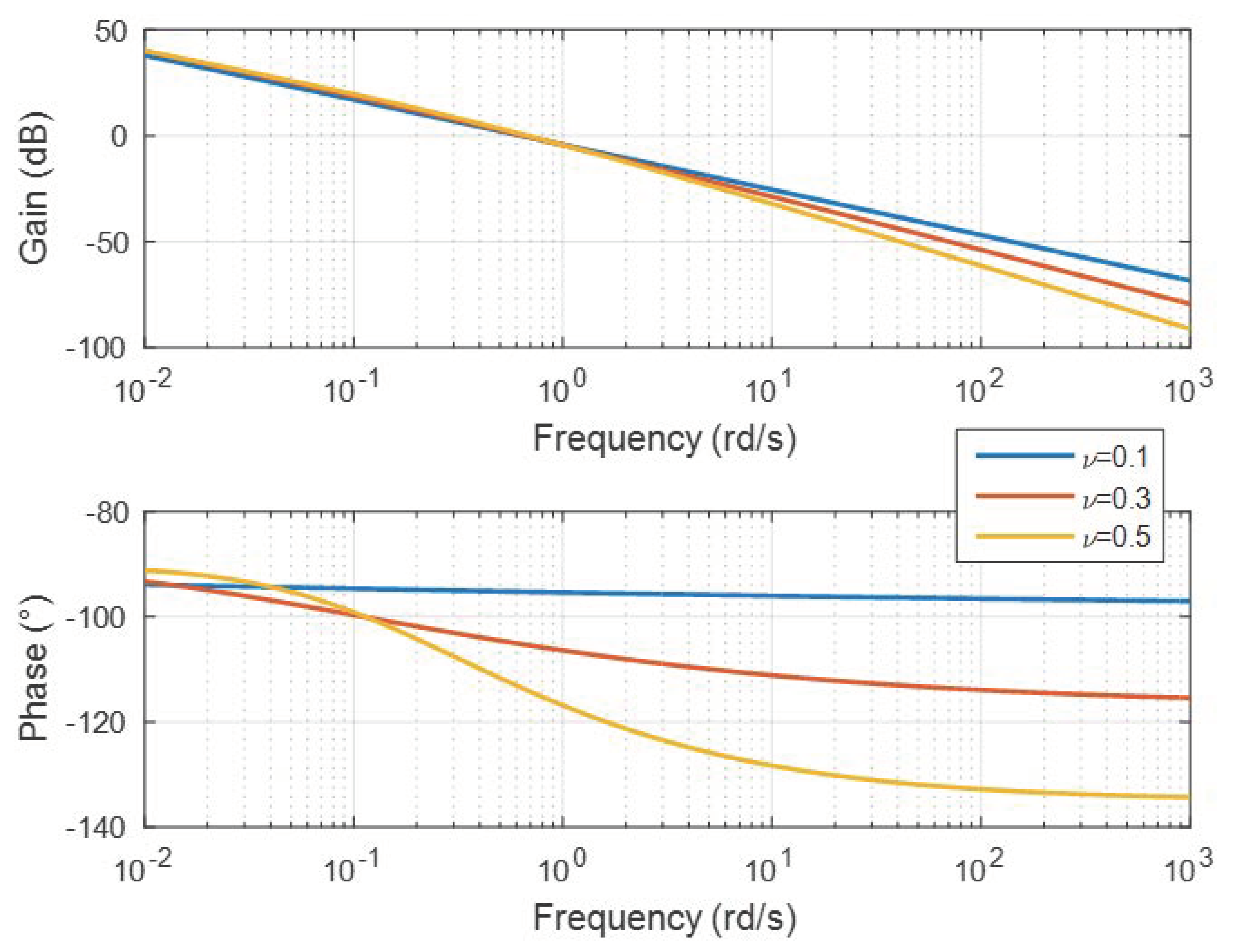
Without referring to fractional models, the Avrami model is often used to model the kinetics of crystallization, in addition to other phase changes or chemical reactions [35,36]. This model is described by the relation:

$$x\left(t\right)=K\left(1-e^{-{\left(at\right)}^{\nu }}\right).$$

(53)

The Laplace transform of Relation (52) is given by:

$$x\left(s\right)=K\left(\frac{1}{s}-\frac{1}{a}{{\displaystyle \sum }}_{r=0}^{\infty }\frac{{\left(-\tau \right)}^r}{r!}\frac{\Gamma \left(1+\nu r\right)}{{\left(\frac{s}{a}\right)}^{1+\nu r}}\right).$$

(54)

Figure 4 shows the frequency response of $x\left(s\right)$ and demonstrates a power-law behavior because the phase is constant and equal to −ν90° for frequencies greater than $a$.

Function $x\left(t\right)$ in Relation (53) is also a solution of the differential equation:

$$\frac{dx\left(t\right)}{dt}=-\mathsf{\nu }{a}^{\nu }{t}^{\nu -1}x\left(t\right)+K\mathsf{\nu }{a}^{\nu }{t}^{\nu -1}.$$

(55)

This equation involves singular coefficients. Such a matter can be solved by a differential equation of the form:

$$\frac{dx\left(t\right)}{dt}=-\mathsf{\nu }{a}^{\nu }{\left(t+c\right)}^{\nu -1}x\left(t\right)+K\mathsf{\nu }{a}^{\nu }{\left(t+c\right)}^{\nu -1} c>0$$

(56)

where $c$ is a constant that also exhibits a power-law behavior and thus shows that time-varying models can capture power-law behaviors.

3.6. Diffusion Equation with Spatially Variable Coefficients

With a judicious choice of the spatial functions $\gamma \left(z\right)$ and $\beta \left(z\right)$, it is shown in [37] that the following heat equation:

$$\frac{\partial T\left(z,t\right)}{\partial t}=\gamma \left(z\right)\frac{\partial }{\partial z}\left(\beta \left(z\right)\frac{\partial T\left(z,t\right)}{\partial z}\right) y\left(t\right)={\frac{\partial T\left(z,t\right)}{\partial z}|}_{z=0} u\left(t\right)=T\left(0,t\right)$$

(57)

generates power-law behaviors. An infinite number of combinations are possible for the functions $\gamma \left(z\right)$ and $\beta \left(z\right)$. This leaves considerable room for theoretical investigations in the search for these functions, prior to the analysis of the properties of Equation (57), and also for the development of methods to identify the functions $\gamma \left(z\right)$ and $\beta \left(z\right)$ based on real data.

4. Concluding Remarks

Fractional operators and the resulting fractional models are known for their memory property. This is an interesting property that makes it possible to capture power-law behaviors that are often encountered in modelling problems. For this class of behaviors, the need exists for models with a memory, but not with an infinite memory; this is unfortunately the case with fractional models. Their infinite memory is demonstrated in this paper by applying mathematical transformations that are described by Figure 5. These transformations highlight that fractional models (described by a fractional differential equation or a pseudo state space description) are fitted with infinitely small and infinitely large time constants. They also describe a fractional model with a diffusion equation defined in an infinite spatial domain. These infinitely large time constants or the infinite spatial domain are precisely the reasons why the models have an infinite memory.

Regrettably, many studies dedicated to fractional models appear to ignore this means of considering fractional models, which leads to errors in how these models are initialized. Due to its infinite memory, it is necessary to consider all of a model’s past, rather than only an initial condition as with the Caputo definition. This is also described in Figure 5.

Fractional models are, however, just one class of models among many that are able to capture power-law behaviors without the drawbacks of fractional models. Other solutions are presented in the paper: operators with limited memory kernels, Volterra equations, distributed time delay models, time-varying models, nonlinear models, and diffusion equations with spatially variable coefficients. Consideration of power-law behaviors without being limited to fractional models provides countless opportunities for research in the field of model analysis and identification.