1. Introduction
Although the normal distribution is used in many fields for symmetrical data modeling, when the data come from a distribution with lighter or heavier tails, the assumption of normality becomes inappropriate. Such circumstances show the need for more flexible models such as the Generalized Normal (GN) distribution [
1], which encompasses various distributions such as the Laplace, normal, and uniform distributions.
In the presence of covariates, the normal linear regression model can be used to investigate and model the relationship between variables, assuming that the observations follow a normal distribution. However, it is well known that a normal linear regression model can be influenced by the presence of outliers [
2,
3]. In these circumstances, as discussed above, it is necessary to use models in which the error distribution presents heavier or lighter tails than normal such as the GN distribution.
Due to its flexibility, the GN distribution is considered a tool to reduce the impact of the outliers and obtain robust estimates [
4,
5,
6]. This distribution has been used in different contexts, with different parameterizations, but the main difficulties to adopting GN distribution modeling have been computational problems since there are no explicit expressions for estimators of the shape parameter. The estimation of the shape parameter should be done through numerical methods. However, in the classical context, there are problems of convergence, as demonstrated in the studies [
7,
8].
In the Bayesian context, the methods presented in the literature for the estimation of the parameters of the GN distribution are restricted and applied to particular cases. West [
9] proved that a scale mixture of the normal distribution could represent the GN distribution. Choy and Smith [
10] used the prior GN distribution for the location parameter in the Gaussian model. They obtained the summaries of the posterior distribution, estimated through the Laplace method, and examined their robustness properties. Additionally, the authors used the representation of the GN distribution as a scale mixture of the normal distribution in random effect models and considered the Markov Chain Monte Carlo method (MCMC) to obtain the posterior summaries of the parameter of interest.
Bayesian procedures for regression models with GN errors have been discussed earlier. Box and Tiao [
4] used the GN distribution from the Bayesian approach in which they proposed robust regression models as an alternative to the assumptions of normality of errors in regression models. Salazar et al. [
11] considered an objective Bayesian analysis for exponential power regression models, i.e., a reparametrized version of the GDN. They derived the Jeffreys prior and showed that such a prior results in an improper posterior. To overcome this limitation, they considered a modified version of the Jeffreys prior under the assumption of independence of the parameters. This assumption does not hold since the scale and the shape parameters correlate with the proposed distribution. Additionally, the use of the Jeffreys prior is not appropriate in many cases and can cause strong inconsistencies and marginalization paradoxes (see Bernardo [
12], p. 41).
Reference priors, also called objective priors, can be used to overcome this problem. This method was introduced by Bernardo [
13] and enhanced by Berger and Bernardo [
14]. For the proposed methodology, the prior information is dominated by the information provided by the data, resulting in a vague influence of the prior distribution. Estimations are made based on priors through the maximization of the expected Kullback–Leibler (KL) divergence between the posterior and prior distributions. The resulting reference prior affords a posterior distribution that has interesting features, such as consistent marginalization, one-to-one invariance, and consistent sampling properties [
12]. Some applications of reference priors can be seen for other distributions in [
15,
16,
17,
18,
19,
20].
In this paper, we considered the reference approach for estimating the parameters of the GN linear regression model. We showed that the reference prior led to a proper posterior distribution, whereas the Jeffreys prior brought an improper one and should not be used. The posterior summaries were obtained via Markov Chain Monte Carlo (MCMC) methods. Furthermore, diagnostic techniques based on the Kullback–Leibler divergence were used.
To exemplify the proposed model, we considered the 1309 entries on the height and diameter of Eucalyptus clones (more details are given in
Section 8). For these data, a linear regression model using the normal distribution for the residuals was not adequate, and so, we used the GN linear regression approach.
This paper is composed as follows.
Section 2 presents the GN distribution with some special cases, and in the following
Section 3, we introduce the GN linear regression model.
Section 4 shows the reference and Jeffreys priors, respectively, for a GN linear regression model. Then, the model selection criteria, in
Section 6, are discussed, as well as their applications.
Section 7 shows the proposed method for analyzing compelling cases considering the Bayesian reference prior approach through the use of the Kullback–Leibler divergence.
Section 8 presents studies with an artificial and a real application, respectively. Finally, we discuss the conclusions in
Section 9.
2. Generalized Normal Distribution
The Generalized Normal distribution (GN distribution) has been referred to in the literature under different names and parametrizations such as the exponential power distribution or the generalized error distribution. The first formulation of this distribution [
1] as a generalization of the normal distribution was characterized by the location, scale, and shape parameters.
Here, we considered the form presented by Nadarajah [
21]. It is understood that the random variable
Y is the GN distribution given its probability density function (pdf) as:
The parameter
is the mean;
is the scale factor; and
s is the shape parameter. In particular, the mean, variance, and coefficient of the kurtosis of
Y are given by:
respectively.
The GN distribution characterizes leptokurtic distributions if
and platykurtic distributions if
. In particular, the GN distribution displays the Laplace distribution when
and the normal distribution when
and
is equal to
, where
is the standard deviation, and when
, the pdf converges to a uniform distribution in (
1).
This distribution is flexible-symmetrical concerning the average and unimodality. Moreover, it allows a more flexible fit for the kurtosis than a normal distribution. Furthermore, the ability of the GN distribution to provide a precise fit for the data depends on its shape.
Zhu and Zinde-Walsh [
22] proposed a reparameterization of the asymmetric exponential power distribution that allows us to observe the effect of the shape parameter on the distribution, which was adapted for the GN distribution. Using a similar reparameterization,
, the GN distribution in (
1) is given by:
The reparametrization above is used throughout the paper.
Figure 1 shows the density functions of the GN distribution in (
2) for various parameter values.
3. Generalized Normal Linear Regression Model
The GN linear regression model is defined as:
where
is the vector of the response for the
ith case,
contains the values of the explanatory variables,
is the vector of regression coefficients, and
is the vector of random errors that follows a GN distribution with mean zero, scale parameter
, and shape parameter
s.
Therefore, the likelihood function is:
The log-likelihood function (
4) is given by:
The first-order derivatives of the log-likelihood function in (
5) are given by:
where
is the digamma function.
The score function obtains the Fisher information matrix. This matrix is helpful to get the reference priors for the model parameters. The following proposition obtains the elements of the Fisher information matrix for the model in (
3).
Proposition 1. Let be the Fisher information matrix, with . The elements of the Fisher information matrix,with and the jth element of , are given by,where and is the trigamma function. The restriction ensures that the elements , calculated for , are finite and the information matrix is positive definite. For further details of this proof, please see Proposition 5 in Zhu and Zinde-Walsh [
22]. Then, Fisher’s information matrix is given by:
The corresponding inverse Fisher’s information matrix is given by:
The matrix in (
9) coincides with the Fisher information matrix found by Salazar et al. [
11] due to the one-to-one invariance property.
4. Objective Bayesian Analysis
An important class of objective priors was introduced by Bernardo [
13] and later developed by Berger and Bernardo [
14]. This class of prior is known as reference priors. A vital feature of the method developed by Berger–Bernardo is the specific treatment given to interest and nuisance parameters. The construction of the reference prior, in the case of nuisance parameters, must be made using an ordered parameterization. The parameter of interest is selected, and the procedure is followed below (see Bernardo [
12], for a detailed discussion).
Proposition 2. (Reference priors under asymptotic normality) Let a probability model with real-valued parameters, and let θ be the quantity of interest. For instance, the posterior distribution of the parameters is asymptotically normal with covariance matrix , where is the upper left submatrix of B, , and is the lower right element of .
Then, it holds that the conditional reference priors can be represented as:and:where and are all proper. A compact approximation will be only required, for the corresponding integrals, if any of those conditional reference priors is not proper. Furthermore, the marginal reference prior of θ is:where . The reference posterior distribution associated with
, after
, is given by:
The proposition is first presented for the presence of one nuisance parameter and further extended to a vector of nuisance parameters (see Bernardo [
12] for a detailed discussion and proofs). Here, as our model has a special structure, we also considered an additional result presented in the following corollary that will be used to construct the reference prior to the GN distribution.
Corollary 1. If the nuisance parameter spaces do not depend on and the functions factorize in the form:then and and there is no need for compact approximations, even if are not proper. Under appropriate regularity conditions (see Bernardo [
12]), the posterior distribution of
is asymptotically normal with mean
, the corresponding MLEs and covariance matrix
, where
and
is the corresponding
Fisher information matrix; in that case,
, and the reference prior may be computed from the elements of Fisher matrix
.
4.1. Reference Prior
The parameter vector
is ordered and divided into three distinct groups, according to their inferential importance. We considered here the case in which
is the parameter of interest and
and
s are the nuisance parameters. To obtain a joint reference prior for the parameters
, and
s, the following ordered parameterization was adopted:
Consider the Fisher matrix in (
9), the inverse Fisher matrix in (10)
, and Corollary 1. Let
; it follows that
Then,
Let
, where
is the upper left
submatrix of
; it follows that
Then,
Finally, let
; it follows that
. Then,
Therefore, a joint reference prior for the ordered parameter is given by:
where
, and
.
Using the likelihood function (
4) and the joint reference prior (
11), we obtain the joint posterior distribution for
, and
s,
The posterior conditional probability densities are given by,
The densities in (
13) and (
15) do not belong to any known parametric family, and the densities in (
14) can be easily reduced to an inverse-gamma distribution form by the transformation
. The parameters of interest were obtained by Monte Carlo methods in a Markov Chain (MCMC). Thus, the posterior densities were evaluated by applying the Metropolis–Hastings algorithm; see, e.g., Chen et al. [
23].
4.2. A Problem with the Jeffreys Prior
The use of the Jeffreys prior in the multiparametric case is often controversial. Bernardo ([
12], p. 41) argued that the use of the Jeffreys prior is not appropriate in many cases and can cause strong inconsistencies and marginalization paradoxes. This prior is obtained from the square root of the determinant of the Fisher information matrix of (
9),
where:
and:
is given by:
Such a prior was also presented in Salazar et al. [
11]. Both priors are from the family of prior distributions represented as:
they are usually improper, and
c is a hyperparameter, while
is the prior related to the shape parameter.
The Jeffreys prior and reference prior are of the form (
17) with, respectively,
The posterior distribution associated with the prior in (
17) is proper if:
where
is the integrated likelihood for
s, given by:
Corollary 2. The marginal prior for s given in Equations (18) and (19) is a continuous function in , and as , we have and . Corollary 3. For , the likelihood function for the parameter s, , under the class of priors (17), is a continuous function bounded in and with complexity when . Proposition 3. The reference prior given in (11) yields a proper posterior distribution, and the Jeffreys prior given in (16) leads to an improper posterior distribution. Therefore, the Jeffreys prior leads to an improper posterior distribution and cannot be used in a Bayesian analysis. Another objective prior known as the maximum data information prior could be considered [
16,
24,
25,
26]; however, such a prior is not invariant under one-to-one transformations, which limits its use. Additionally, the main aim was to consider objective priors. We avoided the use of normal or gamma priors due to the lack of invariance in the parameters. Moreover, the prior may depend on hyperparameters that are not easy to elicit for the GN distributions, and the posterior estimates may vary depending on the included information. Finally, Bernardo [
12] pointed out that the use of our “flat” priors to assign “non-informative” priors should be strongly discouraged because they often result in the suppression of important inappropriate and unjustified assumptions that can easily have a strong influence on the analysis, or even make it invalid.
5. Metropolis–Hastings Algorithm
Here, the Metropolis–Hastings algorithm is considered to sample from
, and
s. In this case, the following conditional distributions are considered:
,
, and
, respectively. On the other hand,
, we considered the following change of variables
for
. This modification leads the parametric space to
, which allows us to sample from the posterior distribution in a more efficient way. Considering the Jacobian transformation, the posterior distribution is given by:
The construction of the Metropolis–Hastings algorithm is done using a random walk for the parameter , for instance the transition is obtained using , where is generated from where and k is a constant that controls the acceptance rate. We have that is the diagonal element of the covariance matrix from the joint posterior distribution of , obtained assuming the maximum a posterior estimate of .
The computational stability was improved considering the logarithm scale. The steps to sample from the posterior distribution are:
Set the values .
Generate from the proposal distribution .
Sample u from a uniform distribution .
If then update from ; otherwise, use the value of , i.e., .
Repeat the same steps above for and .
Repeat Steps 2–5 until we obtain the target sample size.
After we generated the values of
, we computed
. It was assumed that
has the same values for all steps. The value of
k is defined as aiming for the acceptance rate to be between
and
[
27]. To confirm the convergence of the chains, the Geweke diagnostic [
28] was used, as well as graphical analysis.
6. Selection Criteria for Models
In the Bayesian context, there are a variety of criteria that can be adopted to select the best fit between a collection of models. This paper considered the following criteria: the Deviation Information Criterion (DIC) defined by Spiegelhalter et al. [
29] and the Expected Bayesian Information Criterion (EBIC) proposed by Brooks [
30]. These criteria are based on the posterior mean deviation,
, which is the deviation evaluated at the posterior mean of
; thus, it is estimated with
, where the index
q indicates the
realization of a total of
Q realizations and
, where
is the probability density of the GN distribution. The criteria DIC and EBIC are given by:
where
b is the number of parameters in the model and
is the effective number of parameters, defined as
, where
is the mean posterior deviation, which can be estimated as
. Smaller values for the DIC and EBIC indicate the preferred model.
Another widely accepted criterion for model selection is the Conditional Predictive Ordinate (CPO). A detailed description of this selection criterion and the CPO statistic, as well as the applicability of the method for selecting models can be found in Gelfand et al. [
31,
32]. Let
denote the complete data set and
denote the data with the
i-th observation excluded. Consider
for
, the posterior density of
given
. Thus, we can define the
i-th observation of the CPO
by:
where
is the probability density function. High values of CPO
indicate the best model. An estimate for CPO
can be obtained using an MCMC sample of the posterior distribution of
given
,
. For this, let
be a sample of the distribution
, of size
Q. A Monte Carlo approximation of the CPO
[
23] is given by:
A summary statistic of the CPO
’s is
, wherein the higher the value of
B, the better the fit of the model. To illustrate the proposed methodology, a comparison between the normal and GN models is presented in
Section 8.
7. Bayesian Case Influence Diagnostics
One way to observe the influence of observations on a fit of the model is via the global diagnosis; for instance, one can remove some cases from the analysis and analyze the effect of the removal [
33]. The diagnostics of the case influence in a Bayesian perspective are based on the Kullback–Leibler divergence (K-L). Let
denote the K-L divergence between
and
, where
denotes the posterior distribution of
for all data and
denotes the posterior distribution of
without the
i-th case. Specifically,
and therefore,
measures the effect of deleting the
i-th case from the full one on the joint posterior distribution of
. The calibration can be obtained by solving the equation:
where the Bernoulli distribution
is expressed by the parameter
p with success probability[
34] and
is a calibration measure of the K-L divergence. After some algebraic manipulation, the obtained expression is:
bounded by
. Therefore, if
is significantly higher than 0.5, then the
i-th case is influential.
The posterior expectation (
22) can also be written in the form:
where
denotes the expectation from the posterior
. Thus, (
23) can be estimated by using the MCMC methods to achieve the sample from the posterior
. Therefore, if
is a sample of size
Q of
, then:
8. Applications
In this section, the proposed method is illustrated using artificial and real data.
8.1. Artificial Data
An artificial sample of size
was generated in accordance with (
3) with
, and
. The posterior samples were generated by the Metropolis–Hastings technique through the MCMC implemented in the R software [
35]. A single chain of dimensions 300,000 was considered for each parameter, and also, we discarded the first 150,000 iterations (burn-in), aiming to reduce correlation problems. A space with a size of 15 was used, resulting in a final sample size of 10,000. The convergence of the chain was verified by the criterion proposed by Geweke [
28].
Table 1 shows the posterior summaries for the parameters of the GN linear regression model. It can be seen that the estimates were close to the true values, and the
HPD credibility intervals covered the true values of the parameters.
We used the same sample previously simulated to investigate the K-L divergence measure in detecting the GN linear regression model’s influential observations. We selected Cases 50 and 250 for perturbation. For each of these two cases and also considering both cases simultaneously, the response variable was disturbed as follows: , where is the standard deviation of . The MCMC estimates were done similarly to those in the last section. Note that, due to the invariance property, can be computed for the standard GN distribution using the Bayes estimates of and , that is .
To reveal the impact of the influential observations in the estimates of , and s, we calculated the measure of Relative Variation (RV), which was obtained by , where and are the posterior averages of the model parameters considering the original data and perturbed data, respectively.
Table 2 shows the posterior estimates for the artificial data and the RVs of the estimates of the parameters concerning the original simulated data. The data set denoted by (a) consisted of the original simulated data set without perturbation, and the data sets denoted by (b) to (d) consisted of data sets resulting from perturbations in the original simulated data set. Higher values of the relative variations for the parameters
and
s showed the presence of influential points in the data set. However, the estimate of
s did not differ so much from the perturbed Cases (c) and (d).
Considering the samples generated from the posterior distribution of the GN linear regression model parameters, we estimated the measures of the K-L divergence and their respective calibrations for each of the cases considered (a–d), as described in
Section 7. The results in
Table 3 show that for the data without perturbation (a), the selected cases were not influential because they had small values for
and calibration close to
. However, when the data were perturbed (b,d), the values of
were more extensive, and their calibrations were close or equal to one, indicating that these data were influential.
8.2. Real Data Set
In order to illustrate the proposed methodology, recall the Brazilian Eucalyptus clones data set on the height (in meters) and the diameter (in centimeters) of Eucalyptus clones. The data belong to a large pulp and paper company from Brazil. As a strategy for the rising rentability of the forestry enterprise and keeping pulp and paper production under control, the company needs to keep an intensive Eucalyptus clone silviculture. The height of the trees is an important measure for selecting different clone species. Moreover, it is desirable to have trees of similar heights, possibly with a slight variation, and consequently with a distribution function with lighter tails.
The objective is to relate the tree’s diameter (explanatory variable) with its height (response variable). The GN and normal linear regression models were fit to the data via the Bayesian reference process. The posterior samples were generated by the Metropolis–Hastings technique, similar to the simulation study, in which we considered a single chain of dimensions 300,000 for each parameter, with a burn-in of 150,000 iterations; additionally, jumps with a size of 15 were used, resulting in a final sample size of 10,000. The Geweke criteria verified the convergence of the chain.
Table 4 shows the posterior summaries for the parameters of both distributions and the model selection criteria. The GN linear regression model was the most suitable to represent the data as it performed better than the normal linear regression model for all the criteria used. For the fit regression model chosen, note that
was significant, and then, for every one-unit increase in the diameter, the average height of Eucalyptus 0.95 meters increased. In particular, the analysis of the shape parameter (
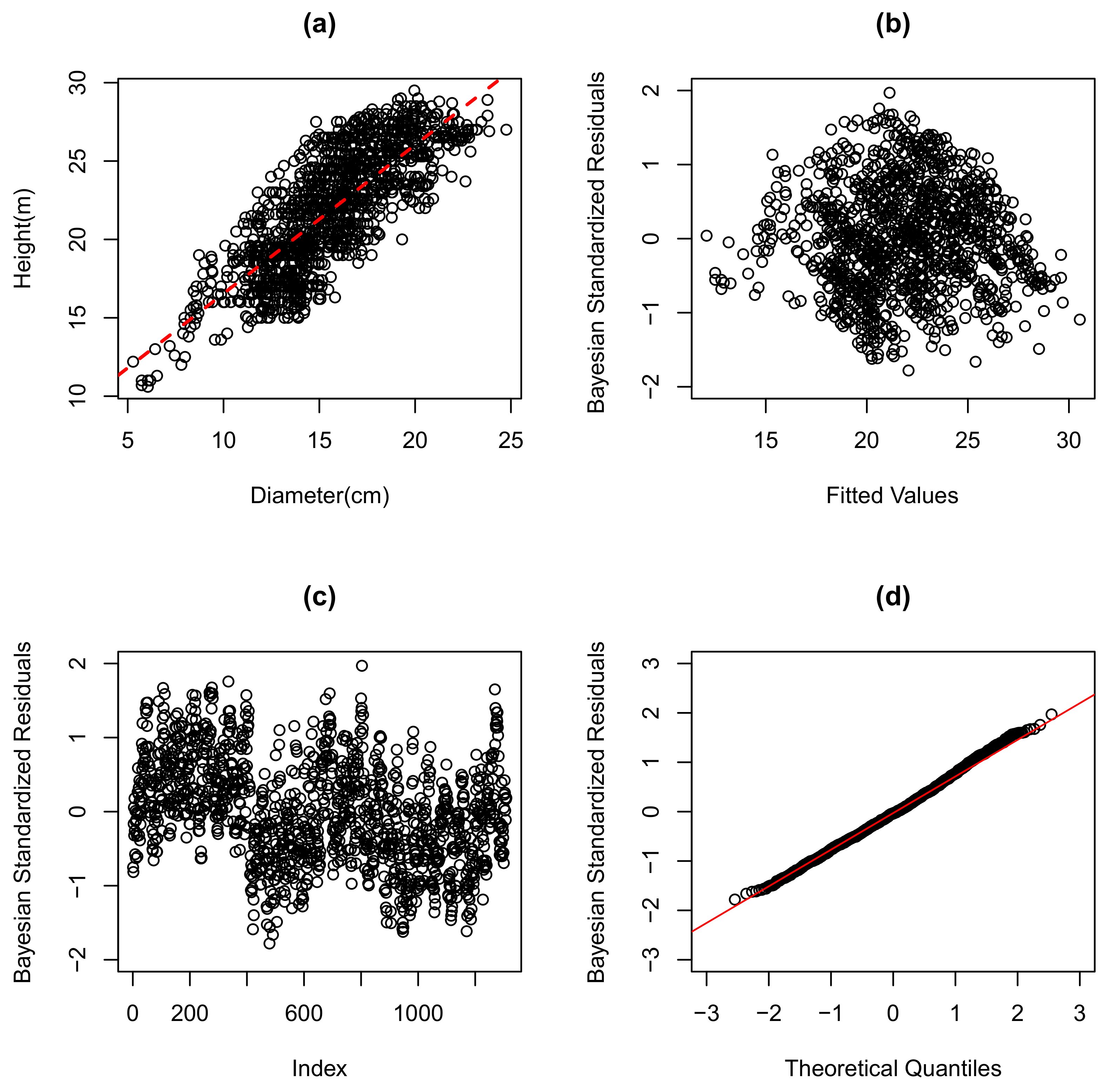
) provided strong evidence of a platykurtic distribution for the errors, and this favored the GN linear regression model. This was further confirmed by graphical analyses of the quantile residuals of the GN linear regression model presented in
Figure 2d.
Figure 2a and
Figure 3a show the scatter plot of the data and the adjusted normal and GN linear regression models. It was observed that, on average, the estimated heights were close to those observed, indicating that the models considered had a good fit. The residuals graph by the fit values and the residuals graph by the observations were also quite similar for both models. The presence of heteroscedasticity (see
Figure 2b and
Figure 3b) was noted, as well as the quadratic trend (see
Figure 2c and
Figure 3c) for the height-to-diameter ratio of the Eucalyptus. The graphs of the quantiles of the GN distribution and the normal distribution for the residuals of the models are presented in
Figure 2d and
Figure 3d, respectively. It can be seen that in the setting of the normal linear regression model, many points were far from their tails, indicating an inadequate specification of the error distribution for the model. On the other hand, using our proposed approach in the GN distribution, we observed a good fit as points were following the line, indicating that the theoretical residuals were close to the observed residuals. Therefore, there was evidence that the model chosen outperformed the normal linear regression model in fitting the data.
To investigate the influence of height and diameter data from Eucalyptus on the fit of the generalized normal linear regression model chosen, we calculated the K-L divergence measures and their respective calibrations.
Figure 4 shows the K-L measurements for each observation. Note that Cases 335, 479, and 803 exhibited higher values of the K-L divergence when compared with other observations. The K-L divergences and calibrations concerning three observations that showed the highest calibration values are presented in
Table 5. It can be seen that Observation 803 was possibly an influential case, which was also shown to be an outlier from the visual analysis. To assess whether this observation altered the parameter estimates of the GN linear regression model, we carried out a sensitivity analysis.
Table 6 shows the new estimates of the model parameters after excluding the case with the greatest calibration value and the relative variations
for these estimates regarding the Eucalyptus data. Here, the relative variations were obtained by
, where
and
are the posterior averages of the model parameters obtained from the original data and from the data without influential observation, respectively. We noted a slight change in the RV of the s parameter when we excluded influential observations. However, such a change was insignificant. This indicated that the GN linear regression model was not affected by the compelling cases.
Overall, regardless of the unit measurement/scale in both cases (synthetic and real data sets), the visual representation corroborated the explainability/adjustment of the GN model, by the quantile-quantile plot, residuals versus fits plot, and standardized errors showing no pattern left to explain equal error variances, as well as no outliers.
9. Discussion
In this paper, we presented the generalized normal linear regression model from objective Bayesian analysis. The Jeffreys prior and reference prior for the generalized normal model were discussed in detail. We proved that the Jeffreys prior leads to an improper posterior distribution and cannot be used in a Bayesian analysis. On the other hand, the reference prior leads to a proper posterior distribution.
The parameter estimates were based on a Bayesian reference analysis procedure via MCMC. Diagnostic techniques based on the Kullback–Leibler divergence were built for the generalized typical linear regression model. Studies with artificial and real data were performed to verify the adequacy of the proposed inferential method.
The result of the application to a set of actual data showed that the generalized normal linear regression model outperformed the normal linear regression model, regardless of the model selection criteria. Furthermore, through a study of artificial data and real data, the Kullback–Leibler divergence effectively detected the points that were influential in the fit of the generalized normal linear regression model. The withdrawal of such influential points from the set of real data showed that the generalized normal model was not affected by influential observations. This result was corroborated by the fact that the generalized normal distribution was considered a tool for reducing outliers and achieving robust estimates. The proposed methodology showed consistent marginalization and sampling properties and thus eliminated the problem of estimating the parameters of this important regression model. Moreover, adopting the reference (objective) prior, we obtained one-to-one consistent results, under the Bayesian paradigm, enabling the GN distribution in a practicalform.
Further works can explore a great number of extensions using this study. For instance, the method developed in this article may be applied to other regression models such as the Student t regression model and the Birnbaum–Saunders regression model, among others. Additionally, other generalizations of the normal distribution should be considered [
36,
37,
38].


 ,
, 


