Bilateral Tempered Fractional Derivatives

Abstract

The bilateral tempered fractional derivatives are introduced generalising previous works on the one-sided tempered fractional derivatives and the two-sided fractional derivatives. An analysis of the tempered Riesz potential is done and shows that it cannot be considered as a derivative.

1. Introduction

In a recent paper [1], we presented a unified formulation for the one-sided Tempered Fractional Calculus, that includes the classic, tempered, substantial, and shifted fractional operators [2,3,4,5,6,7,8,9].

Here, we continue in the same road by presenting a study on the two-sided tempered operators that generalize and include the one-sided. The most interesting is the tempered Riesz potential that was proposed in analogy with the one-sided tempered derivatives [10]. However, a two-sided tempering was introduced before, in the study of the called variance gamma processes [11,12], in Statistical Physics for modelling turbulence, under the concept of truncated Lévy flight [8,13,14,15,16,17], and for defining the Regular Lévy Processes of Exponential type [2,10,18]. The tempered stable Lévy motion appeared in a previous work [19]. Meanwhile, the Feynman–Kac equation used in normal diffusion was generalized for anomalous diffusion and tempered [20,21]. These studies led to the introduction of the tempered Riesz derivative [14] and some applications. Sabzikar et al. [22] described a new variation on the fractional calculus which was called tempered fractional calculus and introduced the tempered fractional diffusion equation. The solutions to this equation are tempered stable probability densities, with semi-heavy tails that state a transition from power law to Gaussian. They proposed a new stochastic process model for turbulence, based on tempered fractional Brownian motion. Li et al. [23] designed a high order difference scheme for the tempered fractional diffusion equation on bounded domain. Their approach is based in properties of the tempered fractional calculus using first order Grünwald type difference approximations. Alternatively, Arshad et al. [24] proposed another difference scheme to solve time–space fractional diffusion equation where the Riesz derivative is approximated by means of a centered difference. They obtained Volterra integral equations which were approximated using the trapezoidal rule. For solving space–time tempered fractional diffusion-wave equation in finite domain another fourth-order technique was proposed in [25,26]. D’Ovidio et al. [27] presented fractional equations governing the distribution of reflecting drifted Brownian motions. In Zhang et al. [28] approximated the tempered Riemann–Liouville and Riesz derivatives by means of second-order difference operator. In [29] new computational methods for the tempered fractional Laplacian equation were introduced, including the cases with the homogeneous and nonhomogeneous generalized Dirichlet type boundary conditions. In [30], by means of a linear combination of the left and right normalized tempered Riemann–Liouville fractional operators, tempered fractional Laplacian (tempered Riesz fractional derivative) was defined as ${(\Delta +\lambda )}^{\beta /2}$. This operator was used to develop finite difference schemes to solve the tempered fractional Laplacian equation that governs the probability distribution function of the positions of particles. Similarly, Duo et al. [31] presented a finite difference method to discretize the d-dimensional (for $d\ge 1$) tempered integral fractional Laplacian ${(-\Delta +\lambda )}^{\alpha /2}$. By means of this approximation they resolved fractional Poisson problems. Hu et al. [32] present the implicit midpoint method for solving Riesz tempered fractional diffusion equation with a nonlinear source term. The Riesz tempered fractional derivative was worked in finite domain. An interesting application of the tempered Riesz derivative in solving the fractional Schrödinger equation was described in [33].

These works suggest us that the tempered Riesz derivative (TRD) is a very important operator. However, and despite such importance, there are no significative theoretical results about such operator. Furthermore, nobody has placed the question: is the tempered Riesz derivative really a derivative?

In this paper, we follow the work described in our previous paper [1] where a deep study on the tempered one-sided derivative was performed. Therefore, we intend here to enlarge the results we obtained previously by combining them with the two-sided derivatives studied in [34]. This approach intends to show that the TRD is not really a fractional derivative according to the criterion introduced in [35]. Instead, we propose a formulation for general tempered two-sided derivatives defined with the help of the Tricomi function [36].

The paper is outlined as follows. In Section 2.1 two preliminary descriptions are done: the one-sided tempered fractional derivatives (TFDs) and the two-sided (non tempered) fractional derivatives (TSFDs). The Riesz–Feller tempered derivatives are introduced and studied in Section 3. Their study in frequency domain shows that they should not be considered as derivatives. The bilateral tempered fractional derivatives (BTFDs) are studied in Section 4. Both versions, continuous- and discrete-time are considered and compared with Riesz-Feller’s. Finally, some conclusions are drawn.

Remark 1.

We adopt here the assumptions in [1], namely

• We work on $\mathbb{R}$.
• We use the two-sided Laplace transform (LT):

  $$F\left(s\right)=\mathcal{L}\left[f\left(t\right)\right]=\underset{\mathbb{R}}{\overset{}{\int }}f\left(t\right)e^{-st}\mathrm{d}t,$$

  (1)

  where $f\left(t\right)$ is any function defined on $\mathbb{R}$ and $F\left(s\right)$ is its transform, provided that it has a non empty region of convergence (ROC).
• The Fourier transform (FT), $\mathcal{F}\left[f\left(t\right)\right]$, is obtained from the LT through the substitution $s=i\kappa ,$ with $\kappa \in \mathbb{R}.$

2. Preliminaries

2.1. The Unilateral Tempered Fractional Derivatives

The one-sided (unilateral) Tempered Fractional Derivatives TFD (UTFD) were formally introduced and studied in [1]. In

Table 1. Stable TFD with $\lambda \ge 0$.

Derivative	${}_{\mathit{\lambda }}{\mathit{D}}_{\pm \mathit{\alpha }}^{\mathit{\alpha }}\mathit{f}\left(\mathit{t}\right)$	LT	ROC
Forward Grünwald-Letnikov	$\underset{h\to 0^{+}}{lim}{h}^{-\alpha }{\displaystyle \sum _{n=0}^{\infty }}\frac{{(-\alpha )}_n}{n!}{e}^{-n\lambda h}f(t-nh)$	${(s+\lambda )}^{\alpha }$	$Re\left(s\right)>-\lambda$
Backward Grünwald-Letnikov	$\underset{h\to 0^{+}}{lim}{h}^{-\alpha }{\displaystyle \sum _{n=0}^{\infty }}\frac{{(-\alpha )}_n}{n!}{e}^{-n\lambda h}f(t+nh)$	${(-s+\lambda )}^{\alpha }$	$Re\left(s\right)<\lambda$
Regularised forward Liouville	${\int }_0^{\infty }\left[f(t-\tau )-\epsilon \left(\alpha \right){\sum }_0^N\frac{{(-1)}^m{f}^{\left(m\right)}\left(t\right)}{m!}{\tau }^m\right]e^{-\lambda \tau }\frac{{\tau }^{-\alpha -1}}{\Gamma (-\alpha )}d\tau$	${(s+\lambda )}^{\alpha }$	$Re\left(s\right)>-\lambda$
Regularised backward Liouville	${\int }_0^{\infty }\left[f(t+\tau )-\epsilon \left(\alpha \right){\sum }_0^N\frac{f^{\left(m\right)}\left(t\right)}{m!}{\tau }^m\right]e^{-\lambda \tau }\frac{{\tau }^{-\alpha -1}}{\Gamma (-\alpha )}d\tau$	${(-s+\lambda )}^{\alpha }$	$Re\left(s\right)<\lambda$

we depict the most important characteristics of the most interesting derivatives, namely the transfer function and corresponding region of convergence (ROC). The tempering parameter $\lambda$ is assumed to be a nonnegative real number. We present only the stable derivatives. This stability manifests in the fact that the ROC of the LT of stable TFD include the imaginary axis. Therefore, the corresponding FT exist and are obtained by setting $s=i\kappa .$ The ROC abscissa is $-\lambda$ in the causal (forward) and $\lambda$ in the anti-causal (backward) cases. The parameter $\alpha \in \mathbb{R}$ is the derivative order and $N=\lfloor \alpha \rfloor$.

Relatively to [1], a complex factor in the backward derivatives was removed to keep coherence with the mathematical developments presented below. The corresponding LT was changed accordingly. Throughout the paper, we will use the designations “Grünwald–Letnikov” (GL) and “Liouville derivative” (L) for the cases corresponding to $\lambda =0$.

2.2. The Two-Sided Fractional Derivatives

Definition 1.

In [34], we introduced formally a general two-sided fractional derivative (TSFD), ${}_0{D}_{\theta }^{\beta },$ through its Fourier transform

$$\mathcal{F}\left[{}_0{D}_{\theta }^{\beta }f\left(x\right)\right]={\left|\kappa \right|}^{\beta }{e}^{i\frac{\pi }{2}\theta ·sgn\left(\kappa \right)}F\left(\kappa \right),$$

(2)

where β and θ are any real numbers that we will call derivative order and asymmetry parameter, respectively.

The inverse Fourier transform computation of (2) is not important here (see, [34]). In

Table 2. TSFD ($\lambda =0$).

Derivative	${}_0{\mathit{D}}_{\mathit{\theta }}^{\mathit{\beta }}\mathit{f}\left(\mathit{t}\right)$	FT
TSGL symmetric	${lim}_{h\to 0^{+}}{h}^{-\beta }{\sum }_{n=-\infty }^{+\infty }\frac{{(-1)}^n\Gamma (\beta +1)}{\Gamma (\frac{\beta }{2}-n+1)\Gamma (\frac{\beta }{2}+n+1)}f(x-nh)$	${\left|\kappa \right|}^{\beta }$
TSGL anti-symmetric	${lim}_{h\to 0^{+}}{h}^{-\beta }{\sum }_{n=-\infty }^{+\infty }\frac{{(-1)}^n\Gamma (\beta +1)}{\Gamma (\frac{\beta +1}{2}-n+1)\Gamma (\frac{\beta -1}{2}+n+1)}f(x-nh)$	$i{\left|\kappa \right|}^{\beta }sgn\left(\kappa \right)$
TSGL general	${lim}_{h\to 0^{+}}{h}^{-\beta }{\sum }_{n=-\infty }^{+\infty }\frac{{(-1)}^n\Gamma (\beta +1)}{\Gamma (\frac{\beta +\theta }{2}-n+1)\Gamma (\frac{\beta -\theta }{2}+n+1)}f(x-nh)$	${\left|\kappa \right|}^{\beta }{e}^{i\frac{\pi }{2}\theta ·sgn\left(\kappa \right)}$
Riesz derivative	$\frac{1}{2cos\left(\beta \frac{\pi }{2}\right)\Gamma (-\beta )}{\int }_{-\infty }^{\infty }\left[f(x-y)-2{\sum }_{k=0}^M\frac{f^{\left(2k\right)}\left(x\right)}{\left(2k\right)!}{y}^{2k}\right]{\left|y\right|}^{-\beta -1}dy,$	${\left|\kappa \right|}^{\beta }$
Feller derivative	$\frac{1}{2sin\left(\beta \frac{\pi }{2}\right)\Gamma (-\beta )}{\int }_{-\infty }^{\infty }\left[f(x-y)-2{\sum }_{k=0}^M\frac{f^{(2k+1)}\left(x\right)}{(2k+1)!}{y}^{2k+1}\right]{\left|y\right|}^{-\beta -1}sgn\left(y\right)dy$	$i{\left|\kappa \right|}^{\beta }sgn\left(\kappa \right)$
Riesz-Feller potential	$\frac{1}{2sin\left(\beta \pi \right)\Gamma (-\beta )}{\int }_{\mathbb{R}}f(x-y)sin\left[(\beta +\theta ·sgn(y\left)\right)\pi /2\right]{\left|y\right|}^{-\beta -1}dy$	${\left|\kappa \right|}^{\beta }{e}^{i\frac{\pi }{2}\theta ·sgn\left(\kappa \right)}$

we present the most interesting definitions of the two-sided derivatives together with the corresponding Fourier transform. It is important to note that we present the regularised Riesz and Feller derivatives.

Some properties of this definition can be drawn [34,37,38]. Here we are mainly interested in the folowing

• Eigenfunctions
  Let $f\left(x\right)=e^{i\kappa x},\kappa ,x\in \mathbb{R}.$ Then

  $${}_0{D}_{\theta }^{\beta }{e}^{i\kappa x}={\left|\kappa \right|}^{\beta }{e}^{i\frac{\pi }{2}\theta ·sgn\left(\kappa \right)}{e}^{i\kappa x},$$

  (3)

  meaning that the sinusoids are the eigenfunctions of the TSFD.
• The Liouville and GL derivatives as particular cases
  With $\theta =\pm \beta$ we obtain the forward (left) (+) and backward (−) Liouville one-sided derivatives:

  $$\mathcal{F}\left[{}_0{D}_{\pm \beta }^{\beta }f\left(x\right)\right]={\left(\pm \kappa \right)}^{\beta }F\left(\kappa \right).$$

  (4)
• The Riesz and Feller derivatives as special cases

  $$\mathcal{F}\left[{}_0{D}_0^{\beta }f\left(x\right)\right]={\left|\kappa \right|}^{\beta }F\left(\kappa \right),$$

  (5)

  and

  $$\mathcal{F}\left[{}_0{D}_1^{\beta }f\left(x\right)\right]=i{\left|\kappa \right|}^{\beta }·sgn\left(\kappa \right)F\left(\kappa \right).$$

  (6)
• Relations involving the sum/difference of Liouville derivatives [39]
  Let $\kappa ,\beta \in \mathbb{R}.$ It is a simple task to show that

  $$\begin{array}{cc}\hfill {\left|\kappa \right|}^{\beta }& =\frac{{\left(i\kappa \right)}^{\beta }+{(-i\kappa )}^{\beta }}{2cos\left(\beta \frac{\pi }{2}\right)},\beta \ne 1,3,5\cdots \hfill \end{array}$$

  (7)

  $$\begin{array}{cc}\hfill {i\left|\kappa \right|}^{\beta }sgn\left(\kappa \right)& =\frac{{\left(i\kappa \right)}^{\beta }-{(-i\kappa )}^{\beta }}{2sin\left(\beta \frac{\pi }{2}\right)},\beta \ne 2,4,6\cdots \hfill \end{array}$$

  (8)

  which means that the Riesz derivative is, aside a constant, equal to the sum of the left and right Liouville derivatives. Similarly, the Feller derivative is the difference. Then,

  $$\begin{array}{cc}\hfill {}_0{D}_0^{\beta }& =\frac{{}_0{D}_{\beta }^{\beta }+{}_0{D}_{-\beta }^{\beta }}{2cos\left(\beta \frac{\pi }{2}\right)},\beta \ne 1,3,5\cdots \hfill \end{array}$$

  (9)

  $$\begin{array}{cc}\hfill {}_0{D}_1^{\beta }& =\frac{{}_0{D}_{\beta }^{\beta }-{}_0{D}_{-\beta }^{\beta }}{2sin\left(\beta \frac{\pi }{2}\right)},\beta \ne 2,4,6\cdots \hfill \end{array}$$

  (10)
• Relations involving the composition of Liouville derivatives [34]
  The composition of the GL, or L, derivatives in (4) is defined by:

  $$\mathcal{F}\left[{}_0{D}_{{\beta }_1}^{{\beta }_1}{}_0{D}_{-{\beta }_2}^{{\beta }_2}f\left(x\right)\right]={\left(i\kappa \right)}^{{\beta }_1}{\left(-i\kappa \right)}^{{\beta }_2}F\left(\kappa \right).$$

  (11)
  Setting $\beta ={\beta }_1+{\beta }_2$ and $\theta ={\beta }_1-{\beta }_2$ we obtain

  $${\Psi }_{\theta }^{\beta }\left(\kappa \right)={\left(i\kappa \right)}^{{\beta }_1}{\left(-i\kappa \right)}^{{\beta }_2}={\left|\kappa \right|}^{\beta }{e}^{i\frac{\pi }{2}\theta ·sgn\left(\kappa \right)},$$

  (12)

  showing that any bilateral fractional derivative can be considered as the composition of a forward and a backward GL, or L, derivatives.
• The TSFD as a linear combination of Riesz and Feller derivatives [34]

  $${}_0{D}_{\theta }^{\beta }f\left(x\right)=cos\left(\frac{\pi }{2}\theta \right){}_0{D}_0^{\beta }f\left(x\right)+sin\left(\frac{\pi }{2}\theta \right){}_0{D}_1^{\beta }f\left(x\right).$$

  (13)

Therefore, any TSFD can be expressed as a linear combinations of pairs: causal/anti-causal GL, or L, or Riesz/Feller derivatives.

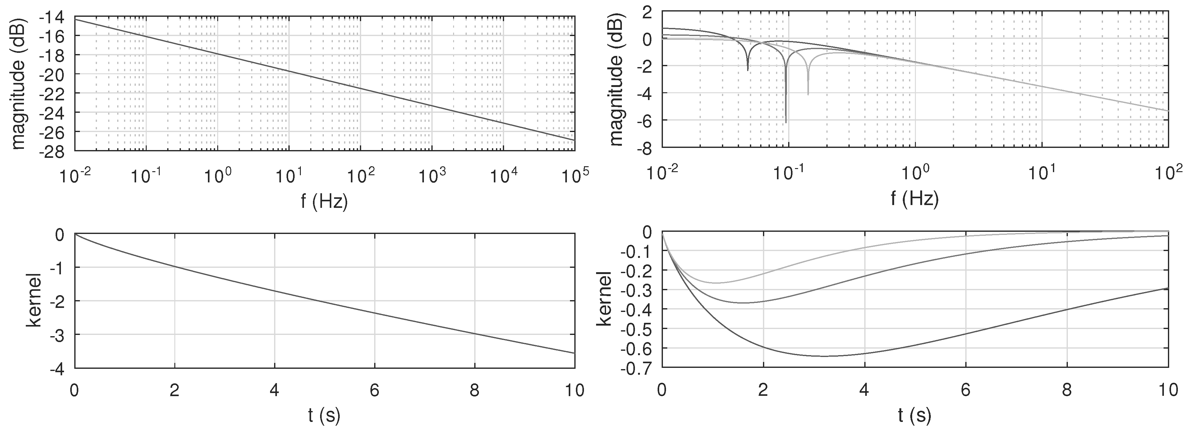
3. Riesz–Feller Tempered Derivatives

The Riesz tempered potential has been used by several authores as referred in Section 1. Here, we will deduce its general regularised form from the TFD in Section 2.1 while using the relation (9).

Definition 2.

We define the tempered Riesz derivative by:

$${}_{\lambda }{D}_0^{\beta }=\frac{{}_{\lambda }{D}_{\beta }^{\beta }+{}_{\lambda }{D}_{-\beta }^{\beta }}{2cos\left(\beta \frac{\pi }{2}\right)}\beta \ne 1,3,5\cdots$$

(14)

This definition allows us to state that

Theorem 1.

$${}_{\lambda }{D}_0^{\beta }f\left(x\right)=\frac{1}{2\Gamma (-\beta )cos\left(\beta \frac{\pi }{2}\right)}{\int }_{-\infty }^{\infty }\left[f(x-\tau )-\sum _{m=0}^M\frac{f^{\left(2m\right)}\left(x\right)}{\left(2m\right)!}{\tau }^{2m}\right]e^{-\lambda \left|\tau \right|}{\left|\tau \right|}^{-\beta -1}d\tau ,$$

(15)

for $2M<\beta <2M+2,M\in {\mathbb{Z}}^{+}$.

Remark 2.

The integer order case leads to a singular situation that we can solve using the relations introduced in [34]. We will not do it here.

Proof. 

We only have to insert the expressions from Table 1 into (14). Let $N=\lfloor \beta \rfloor$ If we use the Liouville derivatives, we obtain:

$$\begin{array}{cc}\hfill {}_{\lambda }{D}_0^{\beta }f\left(x\right)& =\frac{1}{2\Gamma (-\beta )cos\left(\beta \frac{\pi }{2}\right)}{\int }_0^{\infty }\left[f(x-\tau )-\epsilon \left(\beta \right)\sum _{m=0}^N\frac{{(-1)}^m{f}^{\left(m\right)}\left(x\right)}{m!}{\tau }^m\right]e^{-\lambda \tau }{\tau }^{-\beta -1}d\tau \hfill \\ & +\frac{1}{2\Gamma (-\beta )cos\left(\beta \frac{\pi }{2}\right)}{\int }_0^{\infty }\left[f(x+\tau )-\epsilon \left(\beta \right)\sum _0^N\frac{{(+1)}^m{f}^{\left(m\right)}\left(x\right)}{m!}{\tau }^m\right]e^{-\lambda \tau }{\tau }^{-\beta -1}d\tau \hfill \end{array}$$

or

$$\begin{array}{cc}& {}_{\lambda }{D}_0^{\beta }f\left(x\right)=\frac{1}{2\Gamma (-\beta )cos\left(\beta \frac{\pi }{2}\right)}\hfill \\ & {\int }_0^{\infty }\left\{f(x-\tau )+f(x+\tau )-\epsilon \left(\beta \right)\left[\sum _0^N\frac{{(-1)}^m{f}^{\left(m\right)}\left(x\right)}{m!}{\tau }^m+\sum _{m=0}^N\frac{f^{\left(m\right)}\left(x\right)}{m!}{\tau }^m\right]\right\}{e}^{-\lambda \left|\tau \right|}{\left|\tau \right|}^{-\beta -1}d\tau .\hfill \end{array}$$

The odd terms in the inner summation are null. Therefore,

$$\begin{array}{cc}& {}_{\lambda }{D}_0^{\beta }f\left(x\right)=\frac{1}{2\Gamma (-\beta )cos\left(\beta \frac{\pi }{2}\right)}\hfill \\ & {\int }_0^{\infty }\left\{f(x-\tau )+f(x+\tau )-2\epsilon \left(\beta \right)\sum _{m=0}^M\frac{f^{\left(2m\right)}\left(x\right)}{\left(2m\right)!}{\tau }^{2m}\right\}{e}^{-\lambda \left|\tau \right|}{\left|\tau \right|}^{-\beta -1}d\tau .\hfill \end{array}$$

As the integrand is an even function, we are led to (15). □

In which concerns the Laplace and Fourier transforms, we remark that

$$\mathcal{L}\left[{}_{\lambda }{D}_0^{\beta }f\left(x\right)\right]={\displaystyle \frac{{\left(s+\lambda \right)}^{\beta }+{\left(-s+\lambda \right)}^{\beta }}{2cos\left(\beta \frac{\pi }{2}\right)}}F\left(s\right),$$

for $\left|Re\left(s\right)\right|<\lambda ,$ meaning that the ROC is a vertical strip that contains the imaginary axis, $s=i\kappa$. Therefore, as ${\left(\pm i\kappa +\lambda \right)}^{\beta }={\left|{\kappa }^2+{\lambda }^2\right|}^{\frac{\beta }{2}}{e}^{\pm i\beta arctan\left(\frac{\kappa }{\lambda }\right)}$, and using relation (7), we obtain

$$\mathcal{F}\left[{}_{\lambda }{D}_0^{\beta }f\left(x\right)\right]={\displaystyle \frac{{\left|{\kappa }^2+{\lambda }^2\right|}^{\frac{\beta }{2}}cos\left(\beta arctan\left(\frac{\kappa }{\lambda }\right)\right)}{cos\left(\beta \frac{\pi }{2}\right)}}F\left(i\kappa \right),$$

(16)

that is coherent with the usual Riesz derivative ($\lambda =0$).

Definition 3.

Similarly to the Riesz case, we use the relation (10) to find expressions for the tempered Feller derivative that we can define through

$${}_{\lambda }{D}_0^{\beta }=\frac{{}_{\lambda }{D}_{\beta }^{\beta }-{}_{\lambda }{D}_{-\beta }^{\beta }}{2sin\left(\beta \frac{\pi }{2}\right)},\beta \ne 2,4,6\cdots$$

(17)

Theorem 2.

The tempered Feller derivative is given by:

$${}_{\lambda }{D}_0^{\beta }f\left(x\right)=\frac{1}{2\Gamma (-\alpha )sin\left(\beta \frac{\pi }{2}\right)}{\int }_{-\infty }^{\infty }\left[f(x-\tau )-\sum _{m=0}^M\frac{f^{(2m+1)}\left(x\right)}{(2m+1)!}{\tau }^{(2m+1)}\right]e^{-\lambda \left|\tau \right|}{\left|\tau \right|}^{-\beta -1}d\tau ,$$

(18)

for $2M+1<\beta <2M+3$.

The proof is similar to the Riesz derivative. Therefore we omit it.

Now, the corresponding Laplace transform is

$$\mathcal{L}\left[{}_{\lambda }{D}_0^{\beta }f\left(x\right)\right]={\displaystyle \frac{{\left(s+\lambda \right)}^{\beta }-{\left(-s+\lambda \right)}^{\beta }}{2sin\left(\beta \frac{\pi }{2}\right)}},$$

for $\left|Re\left(s\right)\right|<\lambda$. Therefore, using relation (8), we obtain

$$\mathcal{F}\left[{}_{\lambda }{D}_0^{\beta }f\left(x\right)\right]=i{\displaystyle \frac{{\left|{\kappa }^2+{\lambda }^2\right|}^{\frac{\beta }{2}}sin\left(\beta arctan\left(\frac{\kappa }{\lambda }\right)\right)}{sin\left(\beta \frac{\pi }{2}\right)}}F\left(\kappa \right),$$

(19)

that is coherent with the usual Feller derivative ($\lambda =0$). In fact $\underset{\lambda \to 0^{+}}{lim}sin\left(\beta arctan\left(\frac{\kappa }{\lambda }\right)\right)=sin\left[\beta \frac{\pi }{2}\mathit{sgn}\left(\kappa \right)\right].$

Remark 3.

These procedures and the TSGL derivative (3) suggest that the GL type tempered Riesz–Feller derivatives should read

$${}_{\lambda }{D}_0^{\beta }f\left(x\right)=\underset{h\to 0^{+}}{lim}{h}^{-\beta }\sum _{n=-\infty }^{+\infty }\frac{{(-1)}^n\Gamma (\beta +1)}{\Gamma (\frac{\beta +\theta }{2}-n+1)\Gamma (\frac{\beta -\theta }{2}+n+1)}{e}^{-\lambda \left|n\right|h}f(x-nh).$$

(20)

We will not study it, since it leads to the results stated above.

The relation (13) allows us to obtain the general tempered Riesz–Feller derivatives. We only have to insert there the expressions (14) and (18). Proceeding as in [34] we obtain:

Definition 4.

Let $\beta \in \mathbb{R}\backslash \mathbb{Z}$ and $f\left(x\right)$ in $L_1\left(\mathbb{R}\right)$ or in $L_2\left(\mathbb{R}\right)$. The generalised TSFD is defined by

$${}_{\lambda }{\mathcal{D}}_{\theta }^{\beta }f\left(x\right):=\frac{1}{2sin\left(\beta \pi \right)\Gamma (-\beta )}{\int }_{\mathbb{R}}f(x-\tau )sin\left[(\beta +\theta ·sgn(\tau \left)\right)\pi /2\right]e^{-\lambda \left|\tau \right|}{\left|\tau \right|}^{-\beta -1}d\tau .$$

(21)

In terms of the Fourier transform, we have from (13)

$$\mathcal{F}\left[{}_{\lambda }{D}_{\theta }^{\beta }f\left(x\right)\right]=2{\left|{\kappa }^2+{\lambda }^2\right|}^{\frac{\beta }{2}}\left[\frac{cos\left(\theta \frac{\pi }{2}\right)cos\left(\beta arctan\left(\frac{\kappa }{\lambda }\right)\right)}{cos\left(\beta \frac{\pi }{2}\right)}+i\frac{sin\left(\theta \frac{\pi }{2}\right)sin\left(\beta arctan\left(\frac{\kappa }{\lambda }\right)\right)}{sin\left(\beta \frac{\pi }{2}\right)}\right]F\left(\kappa \right).$$

(22)

Remark 4.

It is important to note that none of these operators, tempered Riesz and Feller, and the general Riesz–Feller, can be considered as fractional derivatives. This is easy to see, for example, from (16) that

$${}_{\lambda }{D}_0^{\alpha +\beta }f\left(x\right)\ne {}_{\lambda }{D}_0^{\alpha }{}_{\lambda }{D}_0^{\beta }f\left(x\right),$$

for any pairs $\alpha ,\beta \in \mathbb{R},$ since

$$\begin{array}{cc}\hfill 2{\left|{\kappa }^2+{\lambda }^2\right|}^{\frac{\alpha +\beta }{2}}& cos\left((\alpha +\beta )arctan\left(\frac{\kappa }{\lambda }\right)\right)\ne \hfill \\ \hfill & 2{\left|{\kappa }^2+{\lambda }^2\right|}^{\frac{\alpha }{2}}cos\left[\alpha arctan\left(\frac{\kappa }{\lambda }\right)\right]·2{\left|{\kappa }^2+{\lambda }^2\right|}^{\frac{\beta }{2}}cos\left[\beta arctan\left(\frac{\kappa }{\lambda }\right)\right].\hfill \end{array}$$

(23)

These considerations show that although appealing this way into bilateral tempered fractional derivatives is not correct, since we do not obtain effectively derivatives according to the criteria stated in [35]. In Figure 1, we observe the effect of the tempering on the spectra and on the time kernel corresponding to $\beta =-1.8$ and $\lambda =0,0.25,0.5,0.75.$

4. Bilateral Tempered Fractional Derivatives

Above, we profit the fact that Riesz and Feller derivatives are expressed as sum and difference of one-sided derivatives. However, such approach was not successful, attending to the characteristics of the obtained operators that do not make them derivatives. Anyway, there is an alternative approach.

Definition 5.

We define the Bilateral Tempered Fractional Derivatives (BTFD), ${}_{\lambda }{D}_{\theta }^{\alpha }$, as a composition of forward and backward unilateral TFD derivatives, Liouville or Grünwald–Letnikov. Let a, b, α, and θ be real numbers, such that $\alpha =a+b$ and $\theta =a-b.$ Then

$${}_{\lambda }{D}_{\theta }^{\alpha }f\left(x\right)={}_{\lambda }{D}_a^a\left[{}_{\lambda }{D}_{-b}^{b}f\left(x\right)\right],$$

(24)

or, using the Fourier transform:

$$\begin{array}{cc}\hfill \mathcal{F}\left({}_{\lambda }{D}_{\theta }^{\alpha }f\left(x\right)\right]& ={\left(i\kappa +\lambda \right)}^a{\left(-i\kappa +\lambda \right)}^b\hfill \\ \hfill & ={\left|{\kappa }^2+{\lambda }^2\right|}^{\frac{\alpha }{2}}{e}^{i\theta arctan\left(\frac{\kappa }{\lambda }\right)}F\left(\kappa \right).\hfill \end{array}$$

(25)

It is important to note that ${lim}_{\lambda \to 0^{+}}arctan\left(\frac{\kappa }{\lambda }\right)=\frac{\pi }{2}\mathit{sgn}\left(\kappa \right)$.

Let

$${}_{\lambda }{\psi }_{\theta }^{\alpha }\left(t\right)={\mathcal{F}}^{-1}\left[{}_{\lambda }{\Psi }_{\theta }^{\alpha }\left(\omega \right)\right],$$

(26)

and

$$T\left(\alpha ,\theta ,2\lambda \left|t\right|\right)=\frac{1}{\Gamma \left(-\frac{\alpha +sgn\left(t\right)\theta }{2}\right)\Gamma \left(\frac{\alpha -sgn\left(t\right)\theta }{2}\right)}{\int }_0^{\infty }{e}^{-2\lambda \left|t\right|u}{u}^{-\frac{\alpha +\mathit{sgn}\left(t\right)\theta }{2}-1}{(u+1)}^{-\frac{\alpha -\mathit{sgn}\left(t\right)\theta }{2}-1}du,$$

(27)

closely related (aside a factor) with the Tricomi function [36]. Then

Theorem 3.

For $\alpha ,\beta <0,$

$${}_{\lambda }{\psi }_{\theta }^{\alpha }\left(t\right)=e^{-\lambda \left|t\right|}{\left|t\right|}^{-\alpha -1}T\left(\alpha ,\theta ,2\lambda \left|t\right|\right).$$

(28)

Proof. 

Suppose that $a,b<0.$ As

$${\int }_0^{\infty }f(t+\tau )e^{-\lambda \tau }\frac{{\tau }^{-a-1}}{\Gamma (-a)}d\tau ={\int }_{-\infty }^{0}f(t-\tau )e^{\lambda \tau }\frac{{(-\tau )}^{-a-1}}{\Gamma (-a)}d\tau ,$$

then

$${}_{\lambda }{D}_{\theta }^{\alpha }f\left(t\right)=\left[e^{-\lambda t}{\displaystyle \frac{t^{-a-1}}{\Gamma (-a)}}\epsilon \left(t\right)\right]\ast \left[e^{\lambda t}{\displaystyle \frac{{(-t)}^{-b-1}}{\Gamma (-b)}}\epsilon (-t)\right]\ast f\left(t\right),$$

(29)

where ∗ denotes the usual convolution. Let

$${}_{\lambda }{\psi }_{\theta }^{\alpha }\left(t\right)=\left[e^{-\lambda t}{\displaystyle \frac{t^{-a-1}}{\Gamma (-a)}}\epsilon \left(t\right)\right]\ast \left[e^{\lambda t}{\displaystyle \frac{{(-t)}^{-b-1}}{\Gamma (-b)}}\epsilon (-t)\right].$$

Hence

$${}_{\lambda }{\psi }_{\theta }^{\alpha }\left(t\right)={\int }_0^{\infty }{e}^{-\lambda \tau }{\displaystyle \frac{{\tau }^{-a-1}}{\Gamma (-a)}}{e}^{\lambda (t-\tau )}{\displaystyle \frac{{(\tau -t)}^{-b-1}}{\Gamma (-b)}}\epsilon (\tau -t)d\tau .$$

We have two possibilities

• $t\ge 0$

  $${}_{\lambda }{\psi }_{\theta }^{\alpha }\left(t\right)={\int }_t^{\infty }{e}^{-\lambda \tau }{\displaystyle \frac{{\tau }^{-a-1}}{\Gamma (-a)}}{e}^{\lambda (t-\tau )}{\displaystyle \frac{{(\tau -t)}^{-b-1}}{\Gamma (-b)}}\mathrm{d}\tau ={\int }_0^{\infty }{e}^{-\lambda (\tau +t)}{\displaystyle \frac{{(\tau +t)}^{-a-1}}{\Gamma (-a)}}{e}^{\lambda (-\tau )}{\displaystyle \frac{{\tau }^{-b-1}}{\Gamma (-b)}}d\tau$$
• $t<0$

  $${}_{\lambda }{\psi }_{\theta }^{\alpha }\left(t\right)={\int }_0^{\infty }{e}^{-\lambda \tau }{\displaystyle \frac{{\tau }^{-a-1}}{\Gamma (-a)}}{e}^{\lambda (t-\tau )}{\displaystyle \frac{{(\tau -t)}^{-b-1}}{\Gamma (-b)}}\mathrm{d}\tau ={\int }_0^{\infty }{e}^{-\lambda \tau }{\displaystyle \frac{{\tau }^{-a-1}}{\Gamma (-a)}}{e}^{-\lambda \left(\right|t|+\tau )}{\displaystyle \frac{{(\tau +|t\left|\right)}^{-b-1}}{\Gamma (-b)}}d\tau$$

Setting $a=\frac{\alpha +\theta }{2}$ and $b=\frac{\alpha -\theta }{2}$ we can write

$$\begin{array}{cc}\hfill {}_{\lambda }{\psi }_{\theta }^{\alpha }\left(t\right)& =\frac{e^{-\lambda \left|t\right|}}{\Gamma (-\frac{\alpha +\mathit{sgn}\left(t\right)\theta }{2})\Gamma (-\frac{\alpha -\mathit{sgn}\left(t\right)\theta }{2})}{\int }_0^{\infty }{e}^{-2\lambda \tau }{\tau }^{-\frac{\alpha +\mathit{sgn}\left(t\right)\theta }{2}-1}{(\tau +|t\left|\right)}^{-\frac{\alpha -\mathit{sgn}\left(t\right)\theta }{2}-1}d\tau \hfill \\ & =\frac{{\left|t\right|}^{-\alpha -1}}{\Gamma (-\frac{\alpha +\mathit{sgn}\left(t\right)\theta }{2})\Gamma (-\frac{\alpha -\mathit{sgn}\left(t\right)\theta }{2})}{\int }_0^{\infty }{e}^{-\lambda |t|(1+2\frac{\tau }{\left|t\right|})}{\left(\frac{\tau }{\left|t\right|}\right)}^{-\frac{\alpha +\mathit{sgn}\left(t\right)\theta }{2}-1}{\left(\frac{\tau }{\left|t\right|}+1\right)}^{-\frac{\alpha -\mathit{sgn}\left(t\right)\theta }{2}-1}\frac{d\tau }{\left|t\right|},\hfill \end{array}$$

and

$${}_{\lambda }{\psi }_{\theta }^{\alpha }\left(t\right)=\frac{e^{-\lambda \left|t\right|}{\left|t\right|}^{-\alpha -1}}{\Gamma (-\frac{\alpha +\mathit{sgn}\left(t\right)\theta }{2})\Gamma (-\frac{\alpha -\mathit{sgn}\left(t\right)\theta }{2})}{\int }_0^{\infty }{e}^{-2\lambda \left|t\right|u}{u}^{-\frac{\alpha +\mathit{sgn}\left(t\right)\theta }{2}-1}{(u+1)}^{-\frac{\alpha -\mathit{sgn}\left(t\right)\theta }{2}-1}du.$$

(30)

□

Remark 5.

With (29) we can write

$${}_{\lambda }{D}_{\theta }^{\alpha }f\left(t\right)={\int }_{-\infty }^{\infty }f(t-\tau )e^{-\lambda \left|\tau \right|}{\left|\tau \right|}^{-\alpha -1}T\left(\alpha ,\theta ,2\lambda \left|\tau \right|\right)d\tau ,$$

(31)

that is valid for $\alpha \le 0$. We can extend its validity for $\alpha >0,$ through a regularization as shown above in Section 4. It is important to note the similarity between (31) and (15).

Another version of this derivative can be obtained from the tempered unilateral GL derivatives in Table 1. It has the advantage of not needing any regularization.

Theorem 4.

For any $\alpha ,\theta \in \mathbb{R},$

$${}_{\lambda }{D}_{\theta }^{\alpha }f\left(t\right)=\underset{h\to 0^{+}}{lim}{h}^{-\alpha }\sum _{m=-\infty }^{\infty }{T}_m(\alpha ,\theta ,2\lambda h)e^{-\left|m\right|\lambda h}f(t-mh),$$

(32)

where $T_m(\alpha ,\beta ,2\lambda h)$ is defined below (37).

Proof. 

We have successively

$$\begin{array}{cc}\hfill g\left(t\right)& =\sum _{n=0}^{\infty }\frac{{(-a)}_n}{n!}{e}^{-n\lambda h}\sum _{k=0}^{\infty }\frac{{(-b)}_k}{k!}{e}^{-k\lambda h}f(t-(n-k)h)\hfill \\ & =\sum _{m=-\infty }^{\infty }\left[\sum _{n=max(0,m)}^{\infty }{e}^{-2n\lambda h}\frac{{(-a)}_n}{n!}\frac{{(-b)}_{n-m}}{(n-m)!}{e}^{(m-2n)\lambda h}\right]f(t-mh).\hfill \end{array}$$

Let us work out the series

$$\sum _{n=max(m,0)}^{\infty }{\displaystyle \frac{{(-a)}_n}{n!}}{\displaystyle \frac{{(-b)}_{n-m}}{(n-m)!}}{e}^{(m-2n)\lambda h}.$$

For $m\ge 0$

$$\sum _{n=max(m,0)}^{\infty }{\displaystyle \frac{{(-a)}_n}{n!}}{\displaystyle \frac{{(-b)}_{n-m}}{(n-m)!}}{e}^{(m-2n)\lambda h}=\sum _{n=0}^{\infty }{\displaystyle \frac{{(-a)}_{n+m}}{(n+m)!}}{\displaystyle \frac{{(-b)}_n}{n!}}{e}^{(-m-2n)\lambda h}.$$

(33)

Therefore,

$$\sum _{n=max(m,0)}^{\infty }{\displaystyle \frac{{(-a)}_n}{n!}}{\displaystyle \frac{{(-b)}_{n-m}}{(n-m)!}}{e}^{(-2n+m)\lambda h}=\left\{\begin{array}{c}\sum _{n=0}^{\infty }{\displaystyle \frac{{(-a)}_{n+m}}{(n+m)!}}{\displaystyle \frac{{(-b)}_n}{n!}}{e}^{(-m-2n)\lambda h},m\ge 0\\ \sum _{n=0}^{\infty }{\displaystyle \frac{{(-a)}_n}{n!}}{\displaystyle \frac{{(-b)}_{n-m}}{(n-m)!}}{e}^{(m-2n)\lambda h},m<0\end{array}\right.$$

(34)

Using the relations ${(-a)}_{n+\left|m\right|}={(-a)}_{\left|m\right|}{(-a+|m\left|\right)}_n$ and ${(-b)}_{n+\left|m\right|}={(-b)}_{\left|m\right|}{(-b+|m\left|\right)}_n$ and simplifying, we get

$$\left\{\begin{array}{c}{e}^{-m\lambda h}{\displaystyle \frac{{(-a)}_m}{m!}}\sum _{n=0}^{\infty }{\displaystyle \frac{{(-a+m)}_n}{{(m+1)}_n}}{\displaystyle \frac{{(-b)}_n}{n!}}{e}^{-2n\lambda h},m\ge 0\\ e^{-\left|m\right|\lambda h}{\displaystyle \frac{{(-b)}_{\left|m\right|}}{\left|m\right|!}}\sum _{n=0}^{\infty }{\displaystyle \frac{{(-b+|m\left|\right)}_n}{{\left(\right|m|+1)}_n}}{\displaystyle \frac{{(-a)}_n}{n!}}{e}^{-2n\lambda h},m<0.\end{array}\right.$$

(35)

From this relation, we define a new discrete function $T_m(a,b,2\lambda h)$ by

$$T(a,b,2\lambda h)=\left\{\begin{array}{c}{\displaystyle \frac{{(-a)}_m}{m!}}\sum _{n=0}^{\infty }{\displaystyle \frac{{(-a+m)}_n}{{(m+1)}_n}}{\displaystyle \frac{{(-b)}_n}{n!}}{e}^{-2n\lambda h},m\ge 0\\ {\displaystyle \frac{{(-b)}_{\left|m\right|}}{\left|m\right|!}}\sum _{n=0}^{\infty }{\displaystyle \frac{{(-b+|m\left|\right)}_n}{{\left(\right|m|+1)}_n}}{\displaystyle \frac{{(-a)}_n}{n!}}{e}^{-2n\lambda h},m<0\end{array}\right.$$

(36)

Therefore,

$$g\left(t\right)=\sum _{m=-\infty }^{\infty }{T}_m(a,b,2\lambda h)e^{-\left|m\right|\lambda h}f(t-mh).$$

It is interesting to note that $T_{-m}(a,b,2\lambda h)=T_m(b,a,2\lambda h).$ Setting $\alpha =a+b$ and $\theta =a-b$, we obtain

$$T_m(\alpha ,\theta ,2\lambda h)=\left\{\begin{array}{cc}\frac{{(-\frac{\alpha +\theta }{2})}_m}{m!}\sum _{n=0}^{\infty }{e}^{-2n\lambda h}\frac{{(-\frac{\alpha +\theta }{2}+m)}_n}{{(m+1)}_n}\frac{{(-\frac{\alpha -\theta }{2})}_n}{n!}\hfill & m\ge 0\hfill \\ \frac{{(-\frac{\alpha -\theta }{2})}_{\left|m\right|}}{\left|m\right|!}\sum _{n=0}^{\infty }{e}^{-2n\lambda h}\frac{(-\frac{\alpha -\theta }{2}+{\left|m\right|)}_n}{{\left(\right|m|+1)}_n}\frac{{(-\frac{\alpha +\theta }{2})}_n}{n!}\hfill & m<0.\hfill \end{array}\right.$$

Then

$$T_m(\alpha ,\theta ,2\lambda h)=T_{-m}(\alpha ,-\theta ,2\lambda h),m\in \mathbb{Z}$$

and consequently,

$$T_m(\alpha ,\theta ,2\lambda h)=\frac{{(-\frac{\alpha +\theta }{2})}_{\left|m\right|}}{\left|m\right|!}\sum _{n=0}^{\infty }{e}^{-2n\lambda h}\frac{(-\frac{\alpha +\theta }{2}+{\left|m\right|)}_n}{{\left(\right|m|+1)}_n}\frac{{(-\frac{\alpha -\theta }{2})}_n}{n!},$$

(37)

for any integer $m.$ □

Remark 6.

The similarity of (37) and (27) must be noted.

We can give a more symmentric form of the summation in (37) using a Pfaff transformation, but it seems not to be of particular interest.

To verify the coherence of this result, we note that:

• The second term in (37) is the Hypergeometric function;
• If $\lambda =0$, using a well-known property of the Hypergeometric function, we have

  $$\sum _{n=0}^{\infty }\frac{(-\frac{\alpha +\theta }{2}+{\left|m\right|)}_n}{{\left(\right|m|+1)}_n}\frac{{(-\frac{\alpha -\theta }{2})}_n}{n!}=\frac{\Gamma (1+\alpha )\left|m\right|!}{\Gamma (\frac{\alpha +\theta }{2}+1)\Gamma (\frac{\alpha -\theta }{2}+\left|m\right|+1)},$$

  and,

  $$T_m(\alpha ,\theta ,0)=\frac{{(-\frac{\alpha +\theta }{2})}_{\left|m\right|}}{\left|m\right|!}\frac{\Gamma (1+\alpha )\left|m\right|!}{\Gamma (\frac{\alpha +\theta }{2}+1)\Gamma (\frac{\alpha -\theta }{2}+\left|m\right|+1)}.$$

  (38)
• As ${(1-z)}_n={(-1)}^n\Gamma \left(z\right)/\Gamma (z-n)$,

  $${(-\frac{\alpha +\theta }{2})}_{\left|m\right|}={(-1)}^m\frac{\Gamma (1+\frac{\alpha +\theta }{2})}{\Gamma (\frac{\alpha +\theta }{2}-|m|+1)},$$

  and

  $$T_m(\alpha ,\theta ,0)={(-1)}^m\frac{\Gamma (1+\alpha )}{\Gamma (\frac{\alpha +\theta }{2}-\left|m\right|+1)\Gamma (\frac{\alpha -\theta }{2}+\left|m\right|+1)},$$

  (39)

in agreement with (20). Another interesting result can be obtained by dividing (37) by (38) to obtain the factor

$$Q_m(\alpha ,\theta ,2\lambda h)=\frac{\Gamma (\frac{\alpha +\theta }{2}+1)\Gamma (\frac{\alpha -\theta }{2}+\left|m\right|+1)}{\Gamma (1+\alpha )\left|m\right|!}\sum _{n=0}^{\infty }{e}^{-2n\lambda h}\frac{(-\frac{\alpha +\theta }{2}+{\left|m\right|)}_n}{{\left(\right|m|+1)}_n}\frac{{(-\frac{\alpha -\theta }{2})}_n}{n!},$$

(40)

that expresses the “deviation” of the BTFD from the tempered Riesz–Feller derivative (22). In Figure 2 we illustrate the behavour of this factor for two derivative orders, $\alpha =\pm 0.5$ and three values of the tempering exponent, $\lambda =0.25,0.5,1$ with $\theta =0.4.$ It is important to note that

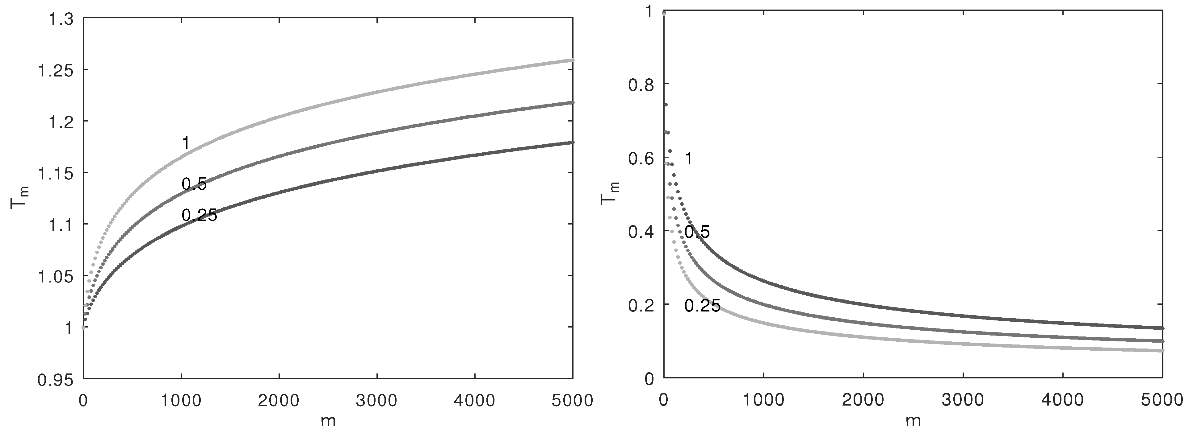
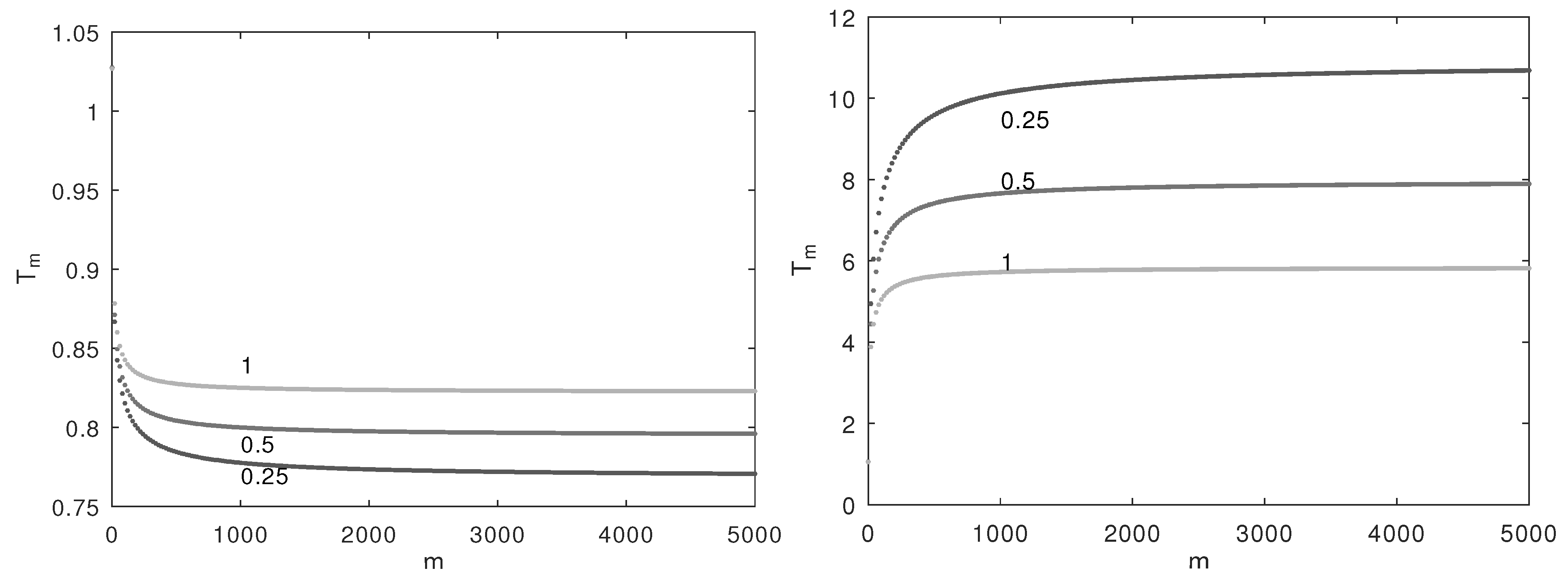
• In the derivative case, $Q_m$ increases slowly and monotonuously with m, contributing for an enlargement of the kernel duration;
• In the anti-derivative case, $Q_m$ decreases slowly and monotonuously to zero with increasing m reducing the kernel duration and consequently the memory of the operator.

Knowing that the first term in (37) tends asymptotically to $\frac{1}{{\left|m\right|}^{\alpha +1}}$ [39], it will be interesting to study the behaviour of the summation term. In Figure 3 we examplify its variation for positive and negative derivative orders for three values of $\lambda$.

As seen, it seems to approach a constant depending on $\lambda$.

Can We Consider the BTFD as Fractional Derivatives?

In Section 4 we noted that the tempered Riesz and Feller potentials could not be considered as fractional derivatives, since the composition property was not valid for any pairs of orders. We wonder if this is also true for the BTFD. We will base our study in the SSC as proposed in [35].

It is not a hard task to show that the BTFD verify the following properties

P1 

Linearity

The BTFD we introduced in the last sub-section is linear.

P2 

Identity

The zero order BTFD of a function returns the function itself, since ${(i\kappa +\lambda )}^0=1$, for any $\lambda ,\kappa \in \mathbb{R}$.

P3 

Backward compatibility

When the order is integer, the BTFD gives the same result as the integer order two-sided TD and recovers the ordinary bilateral derivative, for $\lambda =0$.

P4 

The index law holds

$${}_{\lambda }{D}_{\theta }^{\alpha }{}_{\lambda }{D}_{\eta }^{\beta }f\left(t\right)={}_{\lambda }{D}_{\theta +\eta }^{\alpha +\beta }f\left(t\right),$$

(41)

for any $\alpha$ and $\beta ,$ since

$${\left|{\kappa }^2+{\lambda }^2\right|}^{\frac{\alpha }{2}}{e}^{i\theta arctan\left(\frac{\kappa }{\lambda }\right)}{\left|{\kappa }^2+{\lambda }^2\right|}^{\frac{\beta }{2}}{e}^{i\eta arctan\left(\frac{\kappa }{\lambda }\right)}={\left|{\kappa }^2+{\lambda }^2\right|}^{\frac{\alpha +\beta }{2}}{e}^{i(\theta +\eta )arctan\left(\frac{\kappa }{\lambda }\right)}$$

P5 

The generalised Leibniz rule reads

$${}_{\lambda }{D}_{\theta }^{\alpha }\left[f\left(t\right)g\left(t\right)\right]=\sum _{i=0}^{\infty }\left(\genfrac{}{}{0pt}{}{\alpha }{i}\right)D^{i}f\left(t\right){}_{\lambda }{D}_{\theta }^{\alpha -i}g\left(t\right),$$

(42)

a bit different from the usual. Its deduction is similar to the one described in [1].

We conclude that the BTFD verifies the SSC and therefore can be considered a derivative.

5. Conclusions

This paper addressed the study of tempered two-sided derivatives. Two versions were considered: integral and GL like. The conformity of these operators as studied in the perspective of a criterion for fractional derivatives was stated. In passing we showed that a simple tempering of the traditional Riesz and Feller potentials does not lead to fractional derivatives.

References

- Ortigueira, M.D.; Bengochea, G.; Machado, J.T. Substantial, Tempered, and Shifted Fractional Derivatives: Three Faces of a Tetrahedron. Math. Methods Appl. Sci. 2021, 1–19. Available online: https://onlinelibrary.wiley.com/doi/pdf/10.1002/mma.7343 (accessed on 7 May 2021). [CrossRef]
- Barndorff-Nielsen, O.E.; Shephard, N. Normal modified stable processes. Theory Probab. Math. Stat. 2002, 65, 1–20. [Google Scholar]
- Cao, J.; Li, C.; Chen, Y. On tempered and substantial fractional calculus. In Proceedings of the 2014 IEEE/ASME 10th International Conference on Mechatronic and Embedded Systems and Applications (MESA), Senigallia, Italy, 10–12 September 2014; pp. 1–6. [Google Scholar]
- Chakrabarty, A.; Meerschaert, M.M. Tempered stable laws as random walk limits. Stat. Probab. Lett. 2011, 81, 989–997. [Google Scholar] [CrossRef]
- Hanyga, A.; Rok, V.E. Wave propagation in micro-heterogeneous porous media: A model based on an integro-differential wave equation. J. Acoust. Soc. Am. 2000, 107, 2965–2972. [Google Scholar] [CrossRef]
- Meerschaert, M.M. Fractional calculus, anomalous diffusion, and probability. In Fractional Dynamics: Recent Advances; World Scientific: Singapore, Singapore, 2012; pp. 265–284. [Google Scholar]
- Pilipovíc, S. The α-Tempered Derivative and some spaces of exponential distributions. Publ. L’Institut Mathématique Nouv. Série 1983, 34, 183–192. [Google Scholar]
- Rosiński, J. Tempering stable processes. Stoch. Process. Their Appl. 2007, 117, 677–707. [Google Scholar] [CrossRef]
- Skotnik, K. On tempered integrals and derivatives of non-negative orders. Ann. Pol. Math. 1981, XL, 47–57. [Google Scholar] [CrossRef]
- Carr, P.; Geman, H.; Madan, D.B.; Yor, M. The fine structure of asset returns: An empirical investigation. J. Bus. B 2002, 75, 305–332. [Google Scholar] [CrossRef]
- Madan, D.B.; Milne, F. Option pricing with vg martingale components 1. Math. Financ. 1991, 1, 39–55. [Google Scholar] [CrossRef]
- Madan, D.B.; Carr, P.P.; Chang, E.C. The Variance Gamma Process and Option Pricing. Rev. Financ. 1998, 2, 79–105. Available online: https://engineering.nyu.edu/sites/default/files/2018-09/CarrEuropeanFinReview1998.pdf (accessed on 7 May 2021). [CrossRef]
- Cartea, A.; del Castillo-Negrete, D. Fractional diffusion models of option prices in markets with jumps. Phys. A Stat. Mech. Appl. 2007, 374, 749–763. [Google Scholar] [CrossRef]
- Cartea, A.; del Castillo-Negrete, D. Fluid limit of the continuous-time random walk with general Lévy jump distribution functions. Phys. Rev. E 2007, 76, 041105. [Google Scholar] [CrossRef]
- Mantegna, R.N.; Stanley, H.E. Stochastic Process with Ultraslow Convergence to a Gaussian: The Truncated Lévy Flight. Phys. Rev. Lett. 1994, 73, 2946–2949. [Google Scholar] [CrossRef]
- Novikov, E.A. Infinitely divisible distributions in turbulence. Phys. Rev. E 1994, 50, R3303–R3305. [Google Scholar] [CrossRef]
- Sokolov, I.; Chechkin, A.V.; Klafter, J. Fractional diffusion equation for a power-law-truncated Lévy process. Phys. A Stat. Mech. Appl. 2004, 336, 245–251. [Google Scholar] [CrossRef]
- Carr, P.; Geman, H.; Madan, D.B.; Yor, M. Stochastic Volatility for Lévy Processes. Math. Financ. 2003, 13, 345–382. Available online: https://onlinelibrary.wiley.com/doi/abs/10.1111/1467-9965.00020 (accessed on 7 May 2021). [CrossRef]
- Baeumer, B.; Meerschaert, M.M. Tempered stable Lévy motion and transient super-diffusion. J. Comput. Appl. Math. 2010, 233, 2438–2448. [Google Scholar] [CrossRef]
- Wu, X.; Deng, W.; Barkai, E. Tempered fractional Feynman-Kac equation: Theory and examples. Phys. Rev. E 2016, 93, 032151. [Google Scholar] [CrossRef] [PubMed]
- Hou, R.; Deng, W. Feynman–Kac equations for reaction and diffusion processes. J. Phys. A Math. Theor. 2018, 51, 155001. [Google Scholar] [CrossRef]
- Sabzikar, F.; Meerschaert, M.; Chen, J. Tempered fractional calculus. J. Comput. Phys. 2015, 293, 14–28. [Google Scholar] [CrossRef] [PubMed]
- Li, C.; Deng, W. High order schemes for the tempered fractional diffusion equations. Adv. Comput. Cathematics 2016, 42, 543–572. [Google Scholar] [CrossRef]
- Arshad, S.; Huang, J.; Khaliq, A.; Tang, Y. Trapezoidal scheme for time–space fractional diffusion equation with Riesz derivative. J. Comput. Phys. 2017, 350, 1–15. [Google Scholar] [CrossRef]
- Çelik, C.; Duman, M. Crank–Nicolson method for the fractional diffusion equation with the Riesz fractional derivative. J. Comput. Phys. 2012, 231, 1743–1750. [Google Scholar] [CrossRef]
- Dehghan, M.; Abbaszadeh, M.; Deng, W. Fourth-order numerical method for the space–time tempered fractional diffusion-wave equation. Appl. Math. Lett. 2017, 73, 120–127. [Google Scholar] [CrossRef]
- D’Ovidio, M.; Iafrate, F.; Orsingher, E. Drifted Brownian motions governed by fractional tempered derivatives. Mod. Stochastics Theory Appl. 2018, 5, 445–456. [Google Scholar] [CrossRef]
- Zhang, Y.; Li, Q.; Ding, H. High-order numerical approximation formulas for Riemann-Liouville (Riesz) tempered fractional derivatives: Construction and application (I). Appl. Math. Comput. 2018, 329, 432–443. [Google Scholar] [CrossRef]
- Zhang, Z.; Deng, W.; Karniadakis, G. A Riesz basis Galerkin method for the tempered fractional Laplacian. SIAM J. Numer. Anal. 2018, 56, 3010–3039. [Google Scholar] [CrossRef]
- Zhang, Z.; Deng, W.; Fan, H. Finite Difference Schemes for the Tempered Fractional Laplacian. Numer. Math. Theory Methods Appl. 2019, 12, 492–516. [Google Scholar] [CrossRef]
- Duo, S.; Zhang, Y. Numerical approximations for the tempered fractional Laplacian: Error analysis and applications. J. Sci. Comput. 2019, 81, 569–593. [Google Scholar] [CrossRef]
- Hu, D.; Cao, X. The implicit midpoint method for Riesz tempered fractional diffusion equation with a nonlinear source term. Adv. Differ. Equ. 2019, 2019, 1–14. [Google Scholar] [CrossRef]
- Herrmann, R. Solutions of the fractional Schrödinger equation via diagonalization—A plea for the harmonic oscillator basis part 1: The one dimensional case. arXiv 2018, arXiv:1805.03019. [Google Scholar]
- Ortigueira, M.D. Two-sided and regularised Riesz-Feller derivatives. Math. Methods Appl. Sci. 2019. Available online: https://onlinelibrary.wiley.com/doi/abs/10.1002/mma.5720 (accessed on 7 May 2021). [CrossRef]
- Ortigueira, M.D.; Machado, J.A.T. What is a fractional derivative? J. Comput. Phys. 2015, 293, 4–13. [Google Scholar] [CrossRef]
- Tricomi, F. Sulle funzioni ipergeometriche confluenti. Ann. Mat. Pura Appl. 1947, 26, 141–175. [Google Scholar] [CrossRef]
- Ortigueira, M.D. Riesz potential operators and inverses via fractional centred derivatives. Int. J. Math. Math. Sci. 2006, 2006, 48391. [Google Scholar] [CrossRef]
- Ortigueira, M.D. Fractional central differences and derivatives. J. Vib. Control 2008, 14, 1255–1266. [Google Scholar] [CrossRef]
- Samko, S.G.; Kilbas, A.A.; Marichev, O.I. Fractional Integrals and Derivatives: Theory and Applications; Gordon and Breach Science Publishers: Amsterdam, The Netherlands, 1993. [Google Scholar]