Abstract
The article extends a model-based controller design to higher-order systems, focusing on the speed and shapes of the closed loop responses, including the noise attenuation. It shows that, to obtain simple but reliable results, it is necessary to pay attention to the initial process identification and modelling and also to modify the target closed-loop transfer functions, which must remain causal. To attenuate high initial control signal peaks, appropriate pre-filters are introduced. In order to work with as few parameters as possible, all higher-order transfer functions (process models, target closed loops, pre-filters and noise-attenuation filters) are selected in the form of binomial filters with multiple time constants. Consequently, the so-called “half-rule”, used to reduce too complex process transfer functions, has been modified accordingly. Because derived controllers can lead to different transient dynamics depending on the context of use, the article recalls the need to introduce dynamic classes of control to clarify the mission of individual types of controllers. Consequently, also the performance evaluation using the total variation (TV) criterion had to be refined. Indeed, in its original version, TV is not suitable to distinguish between reasonable and excessive control effort due to improper tuning and noise. The modified TVs allow evaluating higher order systems with multiple changes in direction of their control signal increase without contributing to the excessive control increments. The advantages of the proposed modifications, compared to the traditional approaches, are made clear through simulation examples.
1. Introduction
The development of embedded computers and programmable devices has led to an amazing expansion of applications for automatic control. At the same time, the expansion of embedded solutions also has some drawbacks. Typically, the design aspects in embedded systems are usually much more important than the optimal design of control systems. The reason for this may be the large number of different control approaches that have been developed in the last century. Selecting the most suitable one seems to be a difficult and, above all, time-consuming task. The time required for control loop optimization was quite limited even a few decades ago [1]. Now the situation is even worse under the constant pressure of management deadlines. The problems are also caused by the ever-increasing performance requirements and limits of the improved control devices, which also affect linear PID design to varying degrees. The explosion of various new methods, among them also those of fractional controller design [2,3]) cannot be overlooked, but new solutions can also be documented by the recent revision of SIMC (SImple Control) tuning rules. In the original work [4], for the most frequently used first-order time delayed (FOTD) models [5], the PI controller was predominantly proposed. Recently, IAE optimization-based PID controller modifications have been presented in [6] for this task to increase the achievable performance limits. Moreover, in the context of works dealing with fractional-order PID controllers that eventually lead to implementation by higher-order controllers (HO) [2], or works proposing directly HO derivatives (see, e.g., [7,8,9,10,11] and the references therein), a trend toward using HO controllers is evident. The nice features of the model-based approach were its constructiveness, simplicity and clarity. It coped well with the requirements [4,12] that the controller design should be:
- well motivated,
- preferably model-based,
- analytically derived,
- simple and easy to remember,
- work well for a variety of processes,
- provide fast tracking speed and good disturbance rejection,
- provide stability and robustness with lower variance of process inputs, and
- reduce sensitivity to measurement noise.
However, forced by the ever-increasing requirements for improved performance and robustness of transients, the analysis of the original SIMC design performed in this paper also reveals some ad hoc simplifications. These could be useful for controlling PI, but limit possible generalizations of the approach. The SIMC author has already attempted to improve the method by introducing the iSIMC approach, which, however, somewhat diminishes the advantages of the original analytical design by adding numerical optimization [6].
In addition to the generalization of the model-based SIMC design for higher order systems approximated by the transfer function with a j-tuple time time constant , the original SIMC approach is modified, extended or supplemented in seven other aspects. These include the early stages of controlled process identification, selection of target transfer functions, reduction of more complex process transfer functions to a suitable transfer function , pre-filter design, performance measures used to evaluate the design and its visualization, and design optimization itself.
The choice of the desired first-order closed-loop transfer function for higher-order processes resulted in a noncausal PID controller. Such simplifications complicated the design of the controller, as the realization of appropriate filters needed to implement the controller was far from trivial. By choosing a causal target transfer function, this problem can be avoided: its specification also includes the design of the necessary filters and thus the design of a PID controller is directly comparable to PI.
The mentioned design imbalance between PI and PID controllers is further reduced by a new formulation of the “half-rule”, using an analytical model reduction to simplify more complex transfer functions. A measure of control performance called total variation (TV) has been proposed for the design [4]. Two decades ago, the introduction of TV to evaluate total controller performance was a revolutionary step that demonstrated the need to consider the shape of controller output. However, the limitations of using TV are based on the process orders. Namely, the higher order systems undergo several changes in the direction of the control signal in optimal response. However, such optimal control increases the value of TV and thus deceptively impairs its suitability. Another performance measure to evaluate the speed of transients is the integral of the absolute control error (IAE). Unfortunately, its optimal value usually results in overshoots of the controlled signal. However, these can be unacceptable for many (e.g., mechatronic) applications. To reduce the overshoot, additional design constraints, for example, the sensitivity peaks, were needed. As will be shown later, the aforementioned drawbacks of using both TV and IAE measures can be eliminated by using IAE in combination with modified TV measures based on deviations from the ideal input and output shapes of the system step responses.
Another disadvantage of the original SIMC design is that, with respect to the setpoint step responses, it leads to exaggerated kicks of the control signals to the setpoint changes, even for the simplest solutions. These can lead to the entire control solution being infeasible in practice, especially for lag-dominant systems. Without a suitable design of a pre-filter (reference filter), the control dynamics for setpoint changes can become unacceptable.
After weighing all the problematic aspects, we finally conclude (supported by some recently published works [10,11,13]) that an increase in control performance, robustness and noise suppression can only be achieved by using higher order controllers.
With the aim of addressing the aforementioned trends, the paper is organized as follows. Section 2 builds an internal structure for SIMC design, extends it with pre-filters, and shows that the design is no longer limited to PI and PID controllers, but can be extended to HO controllers even for FOTD plant models. The section also gives some guidance on designing noise filters, modifying the half-rule method, and selection of the desired closed-loop transfer function.
The performance of the modified controller is measured by a refined total variation measure, which is summarized in Section 3. These further allow the modification of the loop optimization to focus on minimizing unnecessary signal increments at both the input and output of the system. The simulation examples given in Section 4, which illustrate the main features and advantages of the newly proposed modifications, are then discussed in Section 5. The final summary and possible further developments of the method are given in the conclusions.
2. Exploring the SIMC Method for Different Plant and Dead-Time Approximations
Figure 1 shows the controller and the process . Before revising the results of the model-based controller design from [4], we first consider the pre-filter . Also, the limitations of the control signal are not yet considered explicitly, but they must be respected at least implicitly. The corresponding closed-loop transfer function between the setpoint and the process output is then
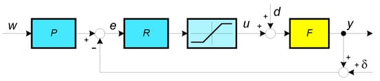
Figure 1.
The controller R and the process F in the closed-loop configuration with a possible control signal limitation; P is the pre-filter, d-disturbance, -measurement noise.
For the given desired closed-loop transfer function , the controller can be calculated from (1) as follows:
Numerous features of such a design have been studied and popularized by [4] in the form of simple analytical rules. The aim of our work is to modify some of its ad hoc features and generalize the above approach so that it can be effectively and reliably applied to higher order processes. In doing so, several steps of the original design need to be revised, including the use of higher-order process models if necessary. Since the modified controller design depends entirely on the order of the process model, the applied model order will be indicated by a superscript before the transfer function, for example, (e.g., when using the second-order process model).
2.1. Controllers Based on FOTD Models
As mentioned earlier, when using the stable first-order time-delay plant (FOTD) models, all associated transfer functions and controllers are denoted by a superscript “1”. For example, expresses the transfer function of the process between its input and its output as:
where is the time delay, K is the plant gain and is the process time constant. Since the process has a time delay, the desired closed loop transfer function between the reference setpoint and the plant output must also include the time delay:
where is the desired closed loop time constant.
Once the desired closed loop transfer function (4) is defined, the controller parameters can be calculated from (2). However, the exponential term (the time delay) appears in the denominator of (2). To solve the equation, the simplest solution is to approximate the exponential term by the first-order Taylor series:
The above approach yields the first-order controller (PI):
where
and where the left index “1” in denotes the order of the process model used to compute the controller parameters, and the right index “1” denotes the controller (in this case PI controller) order. Note that this nomenclature will be used throughout the paper from now on.
As indicated in (7), the integrative time constant and the process model time constant should be positive. This implies that the method can only be applied to stable processes. This restriction also applies to HO controllers.
Note that the recommended values for the closed-loop time constant are [4]:
However, as will be shown later, the above restriction is only a guideline. For the simplest controllers, should be chosen even larger, while it can be reduced for HO controllers. To distinguish the process model parameters () from the actual process parameters (), the subscript “m” is appended to the process parameters in the following text:
Besides developing the exponential term in the denominator of (2) with the first-order Taylor series (5), we can also use the Padé approximation [14]:
In this case, we obtain the following second-order (PID) controller:
where
The controller (11) is briefly discussed in [4], where the conclusion was that “it probably does not justify the increased complexity of the controller and the increased sensitivity to measurement noise”. However, in a recent paper [6], the use of the derivative term is again proposed to improve the closed-loop performance.
Note that (similar to traditional analog controllers) the filter time constant is not arbitrary but uniquely given. Moreover, with the parameters and (12) correspond to the recommended parameters of one of the oldest methods of PID controller tuning [15].
The use of higher order Taylor approximations does not lead to stable controllers, while this is not true for Padé approximations. Indeed, a stable higher order controller is obtained by evolving the exponential term in the denominator of (2) to the second order Padé approximations [14]:
From this approach, the third-order -proportional-integrative-derivative-accelerative () controller is obtained:
where
At this point, the reader may wonder why we should use HO PID controllers when sometimes the PID controllers already have excessive noise gain? As shown in [7,8,9,10,11] and as will be discussed later, the HO controllers can significantly improve control performance even in noisy environments without introducing excessive noise at the controller output. The higher order Padé approximations of the time delay lead to a better description of the controlled system and hence improved control performance. To simplify the further derivations for higher order process models, we will first introduce the normalized dimensionless parameters. By introducing the new time scale defined by the following complex variable:
all other time variables are then related to the time delay (note that ):
Note that in (17), in addition to the normalized process and controller times denoted by the variables , the controller gain is also normalized by the parameter . The controller parameters can then be expressed in a more compact form. For example, the solution (15) can now be expressed as:
In addition to the FOTD process model, the HO models can also be used, as derived in the following subsections.
2.2. Controllers Based on SOTD Models
Remark 1
(The first major change in the SIMC design). The requirement of the first-order closed-loop transfer function for the second-order plant models in [4] leads to an ideal (improper) controller that cannot be realized in practice. This step was probably motivated by the design of PID controllers, prevalent at the time of the mentioned work [4], which did not take into account the calculation of the controller filter. However, such a design violated the requirements of causality, which it complied with only when choosing the appropriate delay of the desired closed-loop transfer function. This also makes the comparison of different controllers under the influence of noise difficult or impossible. Therefore, the mentioned design did not lead to a more efficient design of PID controllers, but resulted in comments such as that the derivative term is difficult to tune [16], that the design is not suitable for noisy and time-delayed processes [1], and that the PI control is preferred because of its simplicity [6].
In view of the problems mentioned in Remark 1, for the second-order time-delayed (SOTD) plant model with a double time constant
the desired closed-loop transfer function obeying controller causality should be
Note that is also a PID controller, but it must be distinguished from the PID controller (11) from the previous section, by index PID and by optimally tuned parameters. The difference between the two types of PID controllers mentioned above is crucial, which was pointed out some time ago [17]. In contrast to the SIMC PID controller, the change in the calculated is obvious. In contrast to the original design, the filter constant is not chosen (e.g., as ), but results directly from the required transfer function . Writing with dimensionless parameters
We get
From the 1st order Padé approximation (10) we obtain the third-order controller
with the dimensionless parameters
Again, we must not forget to distinguish this PIDA controller from PIDA (14) from the previous section. Similarly, we can derive the controller using the 2nd order Padé approximation. To simplify and unify the nomenclature used in the following text, we should replace the traditional abbreviations (PI, PID, or PIDA) with the shorter term R according to the following definition.
2.3. Controller Based on TOTD Models
The third-order time delayed (TOTD) plant model with a triple time constant
with the required closed loop transfer function
and the first-order Taylor approximation (5) yield a solution of (2) in the form of the third-order controller (PIDA controller)
In the dimensionless parameters
As can be seen, the model-based design leads to up to 3 different PIDA controllers, each with a different task and optimal settings. Similarly, we could obtain with the first and with the second-order Padé approximations.
2.4. Controller Based on QOTD Models
The fourth-order time delayed model with a quadruple time constant and dead-time will be defined as
The desired closed-loop transfer function will be chosen as:
Then, considering (2), (5) gives the following fourth-order controller with the 3rd-order derivative action
Such controllers are used, for example, in mechatronics and consider feedback of position, velocity, acceleration and jerk. We could therefore refer to them as PIDAJ.
To control the fourth-order system considered with and denoted as E4 in [4]
Its model order was first reduced by the “half-rule” method. Since, in [4], also the desired closed loop (4) does not satisfy the causality conditions, we will use this example to compare the traditional and modified model-based approaches. In contrast to the ideal PID proposed in [4], the newly proposed solution (32) clearly separates the filter required in (2) (with the time constants ) from a possible additional filter that attenuates the measurement noise. Thus, the proper transfer function simplifies the evaluation and comparison of noise attenuation filters.
2.5. Why Just the Multiple Plant Time Constants?
Definition 2
(jth-order time delayed (jOTD) plant models and the corresponding mth-order R controllers, ). For the sake of simplicity, all the above plant models
used for derivation of R controllers consider just a single j-tuple time constant .
The multiple time constants (see e.g., [18]) have long been used to decrease the number of identified parameters and thus to avoid ill-conditioned identification relationships and simplify their solution. Obviously, by considering not equal stable time constants in , , the family of R controllers could be significantly extended and be more accurate representation of the actual process. However, the controller design should be robust enough to neglect small differences between the time constants of the model, or to reduce the model transfer functions appropriately in the case of higher differences. Therefore, we are going to modify accordingly the original “half-rule”, proposed in [4], used for model reduction.
Additionally, for not equal model time constants, we would also have to select which time constants will be used for the calculation of the controller integral time parameter and which for the calculation of the derivative terms time constants. As has been shown in [19], in constrained control, the properties of the loop with simple anti-windup according to [1] can vary significantly by the mentioned choice of time constants.
2.6. Low-Pass Noise Attenuation Filters
Due to the proportional term, the high frequency noise is not attenuated even in the simplest PI controller. To decrease the noise level, some of works (without giving any arguments) are suggesting using the 2nd-order Butterworth filters [20], while other recommend using the simplest binomial filters at the controller input, or output [21]
With regard to the minimum number of parameters, we will also prefer this second option in this work. The filter will be included in the controller settings using a half-rule and its modification.
2.7. Original Half Rule Method
To satisfy PI and PID controller design, ref. [4] proposed a two-step procedure:
Step 1. Obtain a FOTD or SOTD process model. The effective delay and time constants in this model may be obtained using the half-rule. Thereby, the half-rule was formulated for a mix of different time constants. When simplifying process transfer function including several delays
- the largest neglected (denominator) time constant (lag) has been distributed evenly to the effective delay and the smallest retained time constant,
- the effective delay has summarized (besides of above contribution) the original plant delay and different shorter loop delays.
Step 2. Derive model-based controller settings. The PI controller parameters can be obtained from the FOTD model, whereas the PID controller parameters are calculated from the SOTD model. However, we will further examine how the original HR method supports the design of HO controllers.
Thereby, by the chosen target model transfer function, the strategy of the reduction process is not clearly defined. On the one hand side, by adding half of the neglected time constant to the smallest retained time constant, it seems to decrease differences between the retained (dominant) time constants. However, on the other side, in the reduction process starting with a double dominant plant time constant and an n-fold shorter (filter) time constant with the aim to get a second-order model, Skogestad’s approach would modified just one of the dominant time constants by one half of the neglected filter time constant. Its second half, together with the remaining time constants, would be included into the dead-time. We consider such an increase in the number of mutually different time constants of the process to be unnecessary.
Since from context of the paper [4] one could understand that, preferably, FOTD models and PI controller should be used and for many years, the dominant use of PI controllers only confirmed success of such an approach, we could ignore the previous remark.
2.8. Modified Half Rule for Multiple Time Constants
Note that recently, under denotation “improved SIMC (iSIMC)”, a modified IAE-optimization-based rules [6,22] have been published. They also provide the PID controller (i.e., PID) parameters for FOTD processes. Publication of iSIMC may also be considered as one of the attempts to generalize SIMC rules to HO controllers. However, with respect to FOTD models used, this modification provided no incentive for HR changes. Such motivation arises only when we deal with controllers from branches corresponding to the model of higher orders. (Note, thereby, that, with respect to the chosen branch of controllers, for example, PIDA controller may correspond to PIDA, PIDA or PIDA controller and the reduction process should take these possibilities into account.)
As mentioned above, the effort to minimize the number of loop parameters when working with HO controllers leads us to use simplified system models and noise-attenuation filters with multiple time constants. All these impulses are leading us to a modification of the half-rule (MHR) as follow:
Step 1. Depending on the process type, obtain stable FOTD, SOTD, TOTD, or QOTD (possibly also higher-order) process models. By using the modified half-rule approach (as explained below), the effective time constants and time-delay in the chosen model may be calculated so as to simultaneously design the appropriate controller filter without a limitation on the model order.
Step 2. For the controller branch defined by the considered stable process model, derive the model-based controller settings. The first branch of PI, PID, or PIDA-settings result from a FOTD model. The second branch of controllers (PID, or PIDA) results from the SOTD process model. Similarly, the third branch of controllers (starting with PIDA corresponding to PIDA and possibly continuing to higher-order R controllers) results from TOTD plant models.
Although more accurate solutions can be proposed for the approximation of more complex processes (e.g., by the method of moments according to [23]), with regard to simplicity and tradition the low-pass binomial filters will be included into the plant delay by a modified half-rule (MHR). When starting with j nearly equal dominant time constants and wishing to keep this number, a symmetric distribution of one half of sum of the neglected smaller (possibly n-fold filter time constants) to all the retained j dominant time constants will be preferred. The 2nd half of this sum will be added to dead-time.
Definition 3
(Modified Half Rule (MHR) for jOTD models). When working with a combination of jOTD system (34) with ntuple filter time constant (35), the plant model parameters will be modified to keep a constant open loop average residence time (sum of all delays and time constants) [1]. Furthermore, MHR will symmetrically modify the j-tuple dominant time constant which will be calculated from the identified value according to
Similar to the original HR method, MHR maintains the average residence time (ART) of the system (sum of time constants and delays). However, in the case of an n-fold time constant of a filter, not only one dominant time constant is corrected, but by equal parts all the dominant time constants. The correction is using half of the filter ART , not only half of one of its time constants . As a result, the equivalent dead-time will be shorter than with HR, and the corresponding transients can be faster.
Thereby, such a simplification will be expected to yield expected results just for some limited .
Remark 2
(Conditions for a continuous-time domain application). The continuous-time-domain design methodology can also be applied to today’s mostly digitally implemented controllers, provided that the sampling period used is negligible compared to the smallest filter time constant, that is,
By keeping this requirement, for given hardware limits on and some chosen yielding , the filter order n in (36) will always be limited.
3. Refined Performance Measures
The aim to increase performance of SIMC control unavoidably requires refinement of the performance measures introduced in [4]. In the new setup of the optimal control design [20], one has to deal with a trade-off between speed of control error attenuation (measured usually in terms of integral of absolute error)
Measurement noise injection (influencing primarily the “excessive control effort”, denoted also as controller activity, or input usage, but including possibly also the “output wobbling” [19]) and the robustness.
To avoid undesired effects due to inadequate loop robustness, [6] used in the IAE optimization the sensitivity constraints, as, for example, defined by
Thereby, and represent the peaks of sensitivity functions
which correspond to PI control of a stable plant with .
Despite the fact that the use of and represents one of the pillars of the traditional robust design of PID control, it does not always lead to adequate conclusions [11]. Therefore, we replace the sensitivity constraints in this article with restrictions on the shape of transients at the input and output of the plant.
3.1. Ideal Shapes of Step Responses at the Plant Input and Output
In the era of relay minimum time control of nth-order systems, which brought the first systematic research of optimal control, the requirement to terminate the process in n (rectangular) pulses (control intervals) was used dominantly. It was first mentioned in work by Feldbaum [24]. From this point of view, later formulated modification resulting from maximum/minimum principle [25] brought differences just for the case of systems with complex poles for a large distance between the initial and final states. In the case of jOTD systems with real poles, the conclusions of Feldbaum’s theorem could be formulated in a simplified form and without a proof as:
Theorem 1
(Feldbaum Theorem). For linear systems with j real poles and full relative degree , after a step change of the reference setpoint or the disturbance, the number of control signal intervals required to achieve the neighbourhood of the desired state, with piece-wise alternating control signal limits, is equal to j.
In engineering practice, we approach the minimum-time control only exceptionally. Greater emphasis is placed on smooth continuous changes of the control signal (manipulated variable) and well-damped steady states. In the minimum-time control developed especially for military applications (as missile control, fire control, etc.) the steady-states are frequently not considered. Therefore, due to different priorities, in the literature focused on PID controllers, the Feldbaum’s theorem has been practically forgotten and has rarely been mentioned [26,27]. In addition, when controlling stable systems, the effectively observed number of pulses may be less than the order of the system under consideration. In this respect, it should be noted that with sufficiently smooth and slow processes, it is possible to fill the formulations of the following Lemma:
Lemma 1.
In each Bounded-Input-Bounded-Output (BIBO) stable system, after a step change of the reference setpoint or disturbance, a neighbourhood of the desired state may be achieved with monotonic setpoint step responses of the controller output (plant input) .
Proof.
With regard to a simpler explanation, consider a discrete-time control of a BIBO stable system implemented with some sampling period . For such systems, it is always possible to find (sufficiently small) increments of input such that the corresponding over-regulation (under-regulation) does not exceed an acceptable fraction of the required deviation from monotonicity. After the transient is over, it is possible to add another input increment and wait for the corresponding transient to fade. Thus, by choosing sufficiently slow input increase, it is always possible to achieve (nearly) monotonic plant output response with a monotonic input and to extend such a control also to the continuous-time control with . □
Although, with some exceptions such as above mentioned [26,27], which continued to use Feldbaum’s theorem on optimal control also for smoother control responses, this feature of relay time-optimal controllers dealing with the number of optimal control pulses disappeared from the PID control over time. However, the ever-increasing demands placed on the performance of PID control lead to the fact that when evaluating its dynamics of transients, it will again be necessary to pay attention to control responses obtaining possibly a higher number of pulses. However, due to the requirement of smoothness of processes, these pulses may not be obvious at first glance and thus new performance measures may be required [28]. We will show this on the example of the system (33) (process E4 from [4]), from which we require monotonic closed loop setpoint step response with the time constant shortened from to .
The unit setpoint step responses in Figure 2 illustrate that in order to achieve a smooth monotonic increase of y from initial to final steady state, the course of the first derivative must have one extreme at time and start and end with zero values. However, for the same purpose, the course must have a maximum at some point and a minimum at . As higher derivatives proceed, the number of extremes increases, with maxima alternating with minima and the time of the first maximum gradually decreasing. Finally, in the course of the highest derivative the first monotonic interval between and shrinks to zero. Furthermore, we are no longer able to optically distinguish extremes with higher indices due to high amplitude of initial peak.
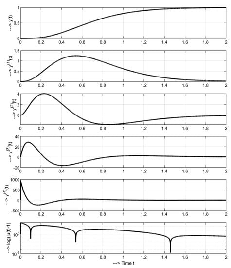
Figure 2.
Unit setpoint step responses of system (33) for with a monotonic increase of the output and four pulses (5 monotonic intervals) of the input , the first interval of increase between and shorten to zero.
The same applies to the course of , which, by alternating increases and decreases, affects the sign of the highest derivative. Therefore, in order to illustrate the increase and decrease of and the corresponding pulses of control with respect to the steady value , the course of can be used. The peaks of this response illustrate the change in the sign of and document that an alternative of the Feldbaum’s theorem can also be formulated for a smooth control signal . However, the decreasing amplitudes of extremes with higher indices, together with the Lemma 1, suggest that nearly optimal responses can also be achieved by simpler control with lower number of pulses.
We encounter similar piece-wise monotonic responses achieved with the same controller when evaluating input disturbance step responses in Figure 3. However, the ideal output response begins with a 1P shape, and the ideal system input is monotonic in this case.
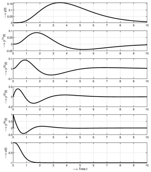
Figure 3.
Unit input disturbance step responses of system (33) for with 1P output and monotonic input .
To simplify the relevant formulations, we will introduce the concept of m-pulse responses in the following.
Definition 4
( function ). Let be a function corresponding to the closed loop control signal of a stable jth-order linear time-delayed system that is:
- continuous for ,
- with possible discontinuity at and
- with initial value and final steady-state value .
Let in a step response can be found for m extremes () lying alternately over and below (or vice versa) the level (as shown in Figure 4) and fulfilling (with the denotation ) conditions
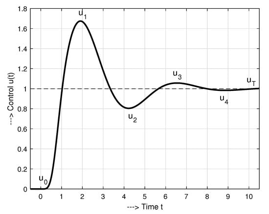
Figure 4.
4P control signal response with extreme values and outlining 5 monotonic intervals.
Then the function , which is monotonic on each of the intervals not containing one of the above extreme points , is called as m-Pulse (mP) function.
In case of discontinuity at , the first extreme point can also be moved to the origin (i.e., , thus shrinking the first monotonic interval between and with to zero.
According to this terminology, monotonic transients can also be referred to as 0P and periodic responses as ∞P functions.
As we will show in the solved examples, the above described model-based control can tend to high initial peaks of the control signal. Such controllers may not be feasible in practice. However, as will be shown later, the initial peaks can be alleviated by a modified controller design.
Definition 5
(Dynamical classes of control). Dynamical class of control DCN [17] is used to denote control with all setpoint step responses given by NP input-0P output pairs . In other words, it denotes setpoint step responses with the plant input consisting of alternately monotonically increasing and decreasing (or vice versa) segments, which are associated with the monotonic plant output .
In the case of the disturbance step responses, it denotes NP input-1P output pairs with the plant input consisting of monotonic segments, which are associated with the plant output consisting of two monotonic response segments.
Thus, setpoint step responses of DC0 includes transients with a monotonic course of the control signal corresponding according to Lemma 1 to a monotonic response at the output. The disturbance step responses of DC0 consist of two monotonic intervals at the output associated with a monotonic change of the control signal.
Similarly, the setpoint step responses of DC2 include control signal transient with 3 monotonic intervals and a monotonic process output response . The disturbance step responses of DC5 consist of two monotonic intervals of the output signal and 6 monotonic intervals of the control signal.
As illustrated by input disturbance step responses in Figure 3, the same controller as considered in Figure 2 may give setpoint and disturbance step responses from fully different dynamical classes.
Definition 6
(Symmetric controller design). A symmetric controller design assumes setpoint and disturbance step responses from the same dynamic class.
The question of the symmetry of the dynamics of setpoint and disturbance responses is of interest to us mainly in terms of their applicability, when at the same controller setting, diametrically different requirements regarding the amplitudes of the control signal may be placed on the actuators. However, it should also be remembered that because the considered model-based approach is based only on the requirements formulated for setpoint responses (1), we can modify the disturbance responses only indirectly.
3.2. Shape Related Performance Measures for Useful/Excessive Output Increments
IAE values used for evaluating speed of the transientsmay be applied both in analytical derivations and in experimental evaluation of the controller design. Since the setpoint step responses can also be improved by an appropriate feedforward, the analysis will preferably focus on the input (load) disturbance step responses given fully by the feedback controller. The achieved responses strongly depend on possible uncertainty of the considered plant model, with an uncertainty impact similar to external disturbances [29]. This gives additional motivation to deal with the disturbance responses, as an indispensable part of the robustness analysis.
Together with the requirement to have the output responses as fast as possible, it is also necessary to consider shapes of actual output and input signals. Thus, although a minimum of (38) usually corresponds to a slight output overshooting, in numerous applications, an ideal setpoint step response has to be monotonic. This corresponds to a situation, when the sum of absolute values of all output increments equals to the net output change specified by the initial and the final values and . Therefore, to characterize the output deviations from monotonicity, the excessive output variation (the total sum of absolute increments [4] reduced by the useful output change) can be used
Such “excessive” increments yield the best view on the “smoothness” of the output response: the ideally smooth monotonic output change corresponds to , else . By limiting the deviations from the monotonicity, we limit also the magnitude of the maximum overshooting, as well as the permanent oscillations of the system.
Similarly as considered in [30] for FOTD plants, an ideal input disturbance step response of the considered stable jOTD plants has always the shape of an one-pulse (1P) curve at the plant output (see in Figure 3). It means that after eliminating imbalance due to a disturbance step change by a corresponding manipulated variable change, the output stops to diverge and then it monotonically returns to the desired reference value. Two monotonic intervals of such a 1P disturbance rejection process are thereby separated by an extreme point and the monotonicity evaluation according to (42) has to be applied twice. Output deviations from an ideal 1P behavior summarize the deviations from monotonicity on these two intervals
In case of several extreme points outside of the strip , the maximal deviation has to be chosen as .
3.3. Shape Related Performance Measures for Useful/Excessive Input Increments
A much more complex situation occurs, when evaluating the optimality of the input variables of the considered stable jOTD plants.
As shown in [28,30], in case of the single integrator the controller output (plant input) corresponding to the setpoint and input disturbance steps have to ideally consist of two monotonic intervals forming an 1P shape (as in Figure 2). Then, similarly as above, deviations of the plant controller output from an ideal 1P step response should be constrained in terms of measures. However, for control of the stable FOTD plants it may be meaningful (see Lemma 1) to consider also input with lower number of control pulses, that is, with a monotonic shape and to consider its evaluation using measure. The decision regarding the choice of or is entirely up to the designer and his subjective evaluation of the specific features of the application.
When it comes to controlling the position of the moving mass represented in mechatronics by integrative second-order models, a 2P (two-pulse) input (similar to in Figure 2) is already needed to achieve a monotonic change in output. It will be dominated with two extremes, one for the acceleration and one for the braking phases. These extremes are separating the total input response into 3 possible monotone sections [31]). Unlike a chain of integrators, when controlling stable 2nd -order systems, the monotonic course of the output can be achieved by 2P, 1P, but also by 0P input.
Similarly, to control a chain of j integrators, an jP type input composed of monotonic sections is needed. However, the situation is complicated by the fact that this time we are not working with integrators, but stable systems, the resulting behavior of which may be more varied and represented by mP functions specified in Definition 4.
Remark 3
(Shape requirements on input of stable jOTD systems). When controlling stable jOTD systems, the input may approach the jP signal (with monotonic intervals) only at high, nearly minimum-time control requirements, which correspond to , a negligible measurement noise and a negligible plant uncertainty. Else, the number of monotonic intervals will be lower, in the limit case just one (with no extreme point). As a result, accurate evaluation of deviations from the ideal input shapes represents an open problem, when controlling stable jOTD systems, since the number of pulses and monotonic segments varies and may be different for the setpoint and disturbance step responses. With a higher level of noise and uncertainty, deviations from monotonicity using , or deviations from the 1P signal using will usually suffice. However, this does not exclude even more complex situations with a higher number of pulses or monotone intervals of the control signal, which makes the use of a TV performance measure in the form introduced in [4] questionable. This evaluates more frequent changes to the control signal as inappropriate and unwanted.
For example, for the transient in Figure 4 with values
The traditional “input usage” evaluation yields traditional and modified total variation values
The deviation from monotonicity would be calculated as . Of course, transients with monotonic input (required for some special applications) may be too slow in a general case. Therefore, frequently a more active control is required. The deviation from 1P response (required typically in PI control) is already much less, just . The deviation from 2P calculated as is yet lower. Similarly, representing deviations from 3P shape. Finally, we may conclude that for the 4th order system, which was under control, the analysed response with represents a fully effective 4P control, without an excessive effort. An optimization process based on TV value would never propose such a solution, even if it is very fast and without excessive control increments. Again, we recall that the decision regarding the choice of a preferred shape related performance measure is entirely up to the designer and his subjective evaluation of the specific features of the application.
Of course, the above calculation refers to ideal waveforms without the influence of measurement noise or imperfect controller settings due to uncertainties, imperfect identification, or time changes of the controlled system. In order to be able to address the influence of individual design factors on the achieved control performance, the evaluation of the circuit will probably need to be divided into several phases.
3.4. First Evaluation Step—Idealized Situation with No Noise
For testing impact of the controller tuning it is recommended to start with an idealized situation without measurement noise and no uncertainties in the plant dynamics. Then, if the control error does not change its sign (which is fulfilled for and ), the IAE values (38) may be calculated as the integral of error (IE). Then, from application of Laplace transform of denoted as follows
For the unit setpoint and input disturbance steps, for all above nominal controllers follows from
values
In ideal situations, with zero shape related deviations at the output, for controllers based on models we get
Thereby, the figure corresponding to the target transfer functions with j-tuple time constants denotes the average residence time (ART) of the closed loop system [1]. This is once more to stress that above formulas hold just in the nominal case. In practical applications, they will also depend on the accuracy of the system model used.
3.5. Optimization Problem
Let us continue with summarizing basic facts:
- Traditional optimization based on quadratic cost functions (LQ control design) does not distinguish useful and excessive signal increments which significantly limits effectiveness of its application.
- Similarly, the use of TV to evaluate control efforts does not distinguish between useful and redundant increments of control signal. This can cause a problem especially when controlling higher order systems and requiring several active impulses of control.
- Separation of the excessive and useful increments (both at the input and output) enables to focus fully on an effective minimization of the superfluous changes.
- In application to evaluation of the setpoint step responses of the plant output , the modified performance measure (42) has a clear mathematical and physical interpretation as a deviation from monotonicity.
- In the new setup of the optimal control design [20], one has to deal with a trade-off between speed of control error attenuation (IAE), measurement noise injection resulting into “excessive control effort” (“controller activity/input usage” [6], or the “output wobbling”) and “robustness”.
- Optimal controller and filter tuning is expected to depend on the noise parameters. Thus, without considering filtration properties, a “generally” optimal PID tuning becomes questionable.
For the loop optimization, different cost functions and different optimization constraints may be defined. A “holistic” loop optimization requiring for the plant model fast and smooth transients, that is, considering both the plant input and output, may be looking for a minimal value of the cost function
By the parameter k it is possible to weight contributions of IAE (speed of control) into the resulting product. The problem remains how to consistently compare the shape of transients proposed using models of different orders j.
A simpler situation occurs during the evaluation with the task to minimize the output wobbling. For the setpoint and disturbance step responses the cost functions may be defined as
Applications of above measures to dominant first-order plants () may be found in [10,11].
3.6. Speed-Effort and Speed-Wobbling Characteristics
Impact of chosen tuning parameters on the trade-off between the speed of control and the shape related deviations at the input and output, may be illustrated by several types of characteristics.
In this paper, they will be based on
- the shape related deviations at the input or output, that is, the measures expressing, how far are the measured transients from their ideally required shapes (variable ) and
- IAE measure characterizing the speed of the control error attenuation (variable )
Dependence of these two basic measures of the closed loop performance, when either
Define two types of the loop characteristics. Into the PID controller design they have been introduced in [32]. Here, they will be denoted as the speed-effort (SE) and speed-wobbling (SW) characteristics.
3.7. IAE-Optimization-Based Tuning of Noisy FOTD Plants
Whereas we may agree with great part of conclusions of [6], one of the basic problems of the IAE-optimization-based “improved” SIMC rules [6] seems to be that, once wishing to be rigorous, the optimization has to be repeated for each new set of parameters of FOTD plant (3) and filter (35). Therefore, it does not allow simple analytical filter consideration. The only possibility is to simplify the plant description (e.g., by application of MHR) up to an integral model. However, such a consideration of the noise attenuation filters (added by the half-rule to the plant dead-time) changes the actual sensitivity values, which again makes use of the optimization-based approaches questionable.
4. Modified Controllers with Reduced Initial Control Signal Peak
One of the shortcomings of the traditional model-based approach is that it does not pay higher attention to the achieved shapes of the control signal responses. Reference [4] only mentions the possibility to avoid derivative kick on setpoint change by following industry practice and differentiating only the output of the system. However, such a solution is not as efficient in terms of adapting the dynamics of the closed-loop responses when compared to pre-filters, or setpoint weighting used in two-degree-of-freedom (2DOF) PID control. We will show that an effective solution to this problem is also related to the actual distribution of dynamic elements of a feedback control system.
As we have already shown above, the model-based design presented in the introductory sections does not provide the same setpoint and disturbance rejection dynamics. During the setpoint step changes, the excessive initial control signal kicks may not be feasible in practice. In further derivations we will show, how to adjust the control signals by using the pre-filters P added to the circuit in Figure 1. We will use an auxiliary system in Figure 5 (firstly with ), which has a clearly defined optimal shapes of the control signal and of a hypothetical output for a setpoint step. This auxiliary system still includes the same jOTD model as considered previously. However, the setpoint response related to its output will be different than it should correspond to the required target closed-loop transfer function
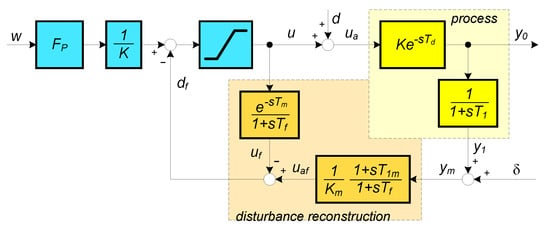
Figure 5.
Static feedforward with input disturbance reconstruction and compensation and a hypothetical process dynamics decomposition into the feedforward and feedback path drawn for a FOTD system; δ-measurement noise.
Finally, we show the impact of modifications of the pre-filter P (e.g., its omission equivalent to ) on the equivalent pre-filter and the shape of the transients in the auxiliary circuit.
Lemma 2
(Equivalence of model-based controllers according to Figure 1 and Figure 5). For stable systems that can be approximated by jOTD model (34) with a j-tuple time constant , an auxiliary control structure with the setpoint and disturbance step responses of DC0 may be specified according to Figure 5 with
This can be transformed to the structure according to Figure 1 with the controllers
and the the pre-filter
Proof.
Given the simplicity and wide use of the PI controller, we start the proof with of (see Figure 5). The constructive approach gives the simplest controller of DC0 for the FOTD plant model in the feedback of the auxiliary system. Thereby, we will not assume that the measured output signal represents directly the controlled output y. In this hypothetical situation considering a memoryless system with a (possibly dominant) transport delay in the direct control branch, that is, with . All explicitly considered (stable) time constants of the jOTD model will be located in the feedback and interpreted as sensor dynamics or noise attenuation filters. Although such a situation seem to be rare in practical applications, in considering both the distribution of the dynamical terms in the loop, as well as the shapes of particular loop signals, it provides a fixed point from which we can start when analyzing shapes of the signals in Figure 1 even at higher values of j. This controller scheme drawn for can be considered as a generalization of the historically first dead-time compensator from Reswick [33].
With a sufficiently long filter time constant preventing exaggerated responses to possible disturbances, after a step change of the reference setpoint signal w, we get both a step change of the controller output and the plant output y, as well as a monotonic (exponential) change of the measured output . Since the step change represents a limit case of monotonic changes, in terms of both considered outputs and , the circuit belongs to DC0 and will remain in it also for the plant time constant moved to the direct branch (i.e., for ).
In a nominal case, with the dead-time estimate and the model time constant , we can denote the observer transfer function based on filtered inversion of the process dynamics as
Estimate of the process dead-time and the used observer filter are included in
For , this control structure provides the closed loop transfer functions
They guarantee both the setpoint and the disturbance responses from DC0. Thereby, tha auxiliary loop has clearly defined shapes of all internal signals corresponding to step inputs: the setpoint steps lead to step changes of and and to an “open-loop” response of . The local loop with a positive feedback via may be replaced (when substituting for (5)) by
Moving from the feedback to the direct branch, merging with and the inverse gain , is then leading with to the controller (6) and (7). The difference, however, is that this time we also got a pre-filter
From the design, which is to compensate for the shift of from the feedback to located in the direct control path. In addition, from (59) we know that for a sufficiently large value of , the disturbance reconstruction will not spoil the step character of the setpoint step responses of the variables u and , whereby remains monotonic. Both the setpoint and the disturbance responses retain the monotonic character even for the time constants located in the direct control branch (i.e., with ).
Next, we derive the design of the controller for the SOTD system (19) and show again that in addition to the controller (21) itself, the design of a suitable pre-filter must also be considered. From the derivation we can then easily come to generalizations for higher order systems.
For a SOTD nominal process (19) in the feedback loop of an auxiliary system with
and for , this control structure provides the closed loop transfer functions
Guaranteeing both the setpoint and the disturbance responses from DC0. Ideally, after a setpoint step, and also show a step change and corresponds to an “open-loop” monotonic response. By replacing the local loop with a positive feedback via we get
Moving from the feedback to the direct branch, merging with and the inverse gain , substituting for (5) and , is then leading to the controller (21). Again, the difference is that this time we also got a pre-filter
In addition, from (64) we know that for a sufficiently large value of , the disturbance reconstruction will not spoil the step character of the setpoint step responses of the variables u and , whereby remains monotonic. Both the setpoint and disturbance responses retain the monotonic character even for both time constants located in the direct control branch (i.e., with ). □
In Lemma 2, the model-based controller design from previous sections derived for jOTD models (34) using the target transfer function (53) has been compared with an auxiliary system with clearly defined shapes of all internal variables. As a result, the control structure of DC0 according to Figure 5 has been shown to be equivalent to the structure according to Figure 1 with the controller and the the pre-filter (56). However, the equivalence assumed a step in the control signal after the setpoint steps, which is far from suitable for all applications. The possibilities of further modifications of setpoint responses are described by the following theorem.
Theorem 2
(Pre-filter design for model-based control). When omitting pre-filter in Figure 1 (i.e., working with , as in SIMC design [4]), although the output of the j-tuple time time constant fulfills behavior prescribed by the target transfer function (53), the control signal may not be feasible for smaller values of . When applying an equivalent change defined by to the auxiliary system, the target transfer function (53) used for design of in the structure according to Figure 1 will be matched by the measured signal in the structure according to Figure 5.
To get smooth setpoint step responses without initial kicks of the control signal, the pre-filter has to be simplified to a strictly proper transfer function. Thereby, by using the same controllers with lower order pre-filters than given by (56), it is possible to speed up the setpoint step responses of the structure according to Figure 1, which then already correspond to a higher dynamic class DCN, .
Proof.
Omitting the pre-filter from the structure in Figure 1 with corresponds to a modified pre-filter . Therefore, it is equivalent to adding the pre-filter to the structure from Figure 5. Then, , and the transfer function matches exactly the target transfer function (4). However, the course will no longer have the shape of a step and, for relatively short values, high peaks with the amplitude may occur in it after unit setpoint steps.
Therefore, where appropriate, the initial kicks of the setpoint step responses of both considered structures may be completely eliminated by using the pre-filters
Definition 7
PI yields smoother monotonic course from DC0, that is, without overshooting, which may be important in design of control respecting given constraints, or in design of systems with hysteresis. The setpoint step response at the output of FOTD model are, however, slower than required by (4). They will not be faster than the open-loop FOTD responses. Two dynamical classes of PI control have been firstly identified in [34].
Experimentally, the monotonic step responses of PI can yet be accelerated by decreasing the pre-filter time constants in (67), which could lead to transients going on with an acceptable overshooting of .
Similarly, for SOTD models, the step character of the setpoint step responses of the structure according to Figure 5 can be replaced with a smoother (but slightly slower) continuous course of by simplifying the pre-filters according to
Definition 8
(PID controllers for lag and dead-time dominant plants).
PID Controller (21) extended according to Figure 1 and Figure 5 by the pre-filters and (68), which at the plant input and output yield setpoint, or monotonic step responses of DC0, may be denoted as PID controllers.
However, PID controllers with monotonic step responses from DC0 can also be designed on the basis of the PID controller (12) supplemented by the pre-filters (67).
While the use of a solution based on SOTD models can be expected to be advantageous for controlling lag-dominant processes, a controller based on FOTD models may appear to be more advantageous for controlling dead-time dominant processes.
As a compromise between (66) and (68) we can choose in the form (68), but of a lower order, thus speeding up the setpoint responses. These can then belong to a higher dynamic class.
We proceed similarly for other values of j (e.g., in designing PIDA controllers), with generalizing multiplicity of the numerator and denominator of the pre-filters (66), or (68) to
Although circuits with relatively large values are the most resistant to uncertainties and noise and do not attack the control signal constraints, it may be interesting to use smaller values. As decreases, the speed of setting the signal to the desired reference value w increases. Situations with monotonic responses achieved under with extremes then correspond to control from a higher dynamic class DCN. This can, however, require to consider control signal constraints and to use appropriate anti-windup schemes [35,36,37,38], or more advanced design methods [39,40]. □
4.1. Integrative Controllers for the Simplest Pure Dead-Time Plant Models
To complement the family of integrative controllers, we will include even simpler process models with pure delay. The control structure in Figure 5 can also be advantageously modified for situations where the time constants can be neglected () when leading to a predictive integrative (I) controller. In such a situation, with a first order reconstruction filter
By omitting the not feasible pre-filters and in the auxiliary circuit according to Figure 5 and in Figure 1, we will replace the step-wise responses of and by smoother exponential transients, which correspond to:
It also means that the tuning parameter is .
For the dead-time approximation (5), the approach gives equivalent loops with I-controller
If we continue in this way using the Padé approximation (10), we get another integrative controller that might be denoted as a filtered PI controller, or I-PD controller given by the equations
It may be used with pre-filters (71).
The 2nd-order Padé approximation (13) yields similarly solution that may be denoted as I-PDD controller
For the pre-filter design applies the same as for the I-controller.
Of course, the solutions based on the elimination of dead-time from the controller structure had its justification in the time of analog controllers. Today, it might be more advantageous to implement this control based on a default scheme with disturbance reconstruction and compensation in Figure 5. Especially in the simplest considered situation, such a “predictive” integrative (I) controller can be significantly more efficient than an I controller. However, it can be effectively and robustly tuned just by the performance portrait method [4,41,42].
4.2. Pre-Filter Design for the SIMC PID Controller
When applying the above procedure to the SIMC PID for the plant according to [4], it must be taken into account that this design leads to an ideal controller (with non-causal target transfer function). Thus, as in Figure 5, the first-order filter is applied, while in the feedback loop, the two time constants and are compensated, that is,
By replacing the inner loop with
moving to a straight branch, merging with and , substituting for (5) and considering , both the pre-filter and the ideal SIMC PID controller can be calculated as:
Practical implementation of the controller requires using the first-order low-pass filter with the time constant [4].
Smoother monotonic responses can again be achieved by selecting the pre-filter according to
The speed of setpoint step responses may be further accelerated with considering just the first-order pre-filter (67).
5. Illustrative Examples
The differences between the traditional SIMC method with HR and the proposed design modifications using MHR, will be illustrated on several examples. For the sake of simplicity, where appropriate, the upper index “1” used to denote PI, PID, or PIDA controller will be omitted.
5.1. Example 1: SIMC and Newly Proposed Control of FOTD System with the 2nd Order Low-Pass Filter
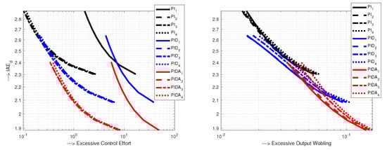
In this example, the 2nd order binomial filter (35) inspired by [27] (with ) has been added to SIMC PI and PID controllers (SPI and SPID) and to all three first-branch controllers (PI, PID and PIDA) based on FOTD models.
According to HR, the SPI and SPID controllers are tuned as follows
For SPID, the derivative action time constant [6] and the series controller filter time constant for noisy processes [4] have been specified according to
According to MHR (36), used in PI, PID and PIDA tuning, the identified plant time constant and the identified plant model dead-time have to be modified according to
Particular loop parameters have been specified as follows:
The required closed loop time constant under the PI controller has been chosen slightly below the recommended (8) with the aim to keep the speed of transients close to PID and PIDA control. Since the PI controller does not include “aggressive” derivative term, the filter time constant may be decreased. PID control, in general, allows faster transients, which is reflected by smaller . However, due to an increased noise level, has been intuitively increased as well. Both mentioned modifications have also been applied on PIDA controller.
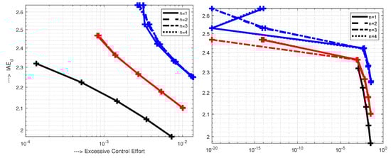
Performance measures , and on unit input step disturbance, for all three controllers (82) are given in Figure 6. For all controllers, values are nearly equal. In terms of , the lowest excessive control effort, when there is no noise (), is achieved with PIDA controller, while the highest effort is obtained with PID controller.
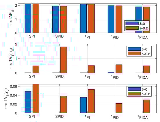
Figure 6.
Performance of the loops with FOTD plant, SIMC PI ad PID controllers (SPI and SPID) tuned for (79), PI (6) and PID (12) and PIDA (15) controllers tuned for model (81). All controllers are using the 2nd order filter (35) with parameters (82). The performance is calculated for no external noise () and for noise amplitudes ; ; ; ; ; .
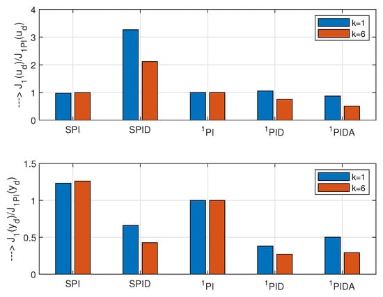
Concerning the process output signal, the PID and PIDA controllers yield nearly ideal 1P responses with . The highest excessive output changes are obtained with the PI control. With existing measurement noise , the output changes are even larger than the ones obtained with the PID and PIDA controllers. For all three controllers, the excessive control effort, due to the measurement noise, significantly exceeds the one without the noise (). Surprisingly, PIDA controller, with the fastest transients and seemingly “aggressive” 2nd order derivative action, shows lower excessive control effort than the simplest and slowest PI control. This is well documented by the combined cost functions (50) and (51) in Figure 7. The normalized values, based on the PI controller, show that the PID controller with has slightly higher value of . However, the PIDA controller’s cost function is lower. The superiority of PID and PIDA control is even more evident when emphasizing the speed of transients (). Obviously, the optimization of the chosen controller and filter tuning is far from being trivial and requires to develop a systemic approach. Given the unlimited range of different requirements of practice (represented by the parameter k), the search for a globally optimal method of controller tuning can therefore be considered erroneous, even when restricted just to simple PID control [43].
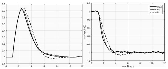
From the noise attenuation point of view, in comparison with SPI and SPID controller, the PI and PID controllers show improved noise attenuation, which is demonstrated (for PID) by lower shape-related deviations in Figure 6, or (for both PI and PID) by the lower values of the cost functions in Figure 7. Transients under noisy process signals are shown in Figure 8. As indicated by increased , under PI control, a relatively short value leads to a moderate output undershooting. Although the amplitude of the noise superimposed according to Figure 1 on the output variable exceeds 25% of the maximal useful signal, on the control variable and even less on the output , its effect is relatively small.
The process output responses, under PID and PIDA controllers, are nearly ideal 1P responses with . Therefore, in the case with no noise we may expect IAE values (49) to be close to the values achieved by simulation. Thus, under PID control with , choosing the equivalent model parameters (81) , we get for (49), which is nearly the same as from simulation. Similarly, for PIDA control with resulting in (81), we get for (49), which is again nearly the same as from simulation. These calculations may be considered as an experimental verification of the applicability of MHR from Definition 3. They also illustrate motivation of [6] to return to the PID control, which was rejected in the initial work [4].
5.2. Example 2:SE/SW Based Analysis of Controller + Filter Tuning—No Noise
The aim of this example is to explain the choice of the parameter in (82) by exploring SE and SW characteristics of the particular controllers with the chosen filters (35).
To get almost constant filter delay for different filter orders n, the filter time constants will be derived by MHR from the filter average residence time according to
Filtered PI control with three different values of yields SE and SW characteristics shown in Figure 9. By increasing the corresponding IAE values increase. Thereby, the curves corresponding to different filter degrees n mostly overlap, which supports simplified filter description (83). To get nearly 1P responses at the plant output for , when , one needs to choose . For it may already be achieved with .
To get nearly 1P transients at the input (not covered by these figures), for and 0.2 one needs to choose and 1.4, respectively. Thus, for PI controller, and desired zero shape related deviations, even when including into the equivalent dead-time, the recommendation (8) is too weak.
Remark 4
(Lag and delay dominant processes). It can be stated that the above conclusions regarding the choice of , to guarantee the smallest possible deviation of responses from their ideal shapes, are in a good agreement with the recommendations of “smoother tuning” in SIMC [6] for PI controller, giving . Of course, the considered process with , does not even represent all stable 1st order processes. However, regarding the choice of , the obtained results can thus be easily interpreted using the ratio or . Furthermore, some other recommendations are anticipated for lag-dominant processes with and still other for delay-dominant with . In this article, however, we will not discuss in detail all possible cases, but we plan to offer the reader an interactive web application, where the particular cases can be easily verified.
PID control (12) inspected for yields nearly 1P output transients for (Figure 10). At the input this happens just for () or (). The value in (82) guarantees ideal shapes just at the output.
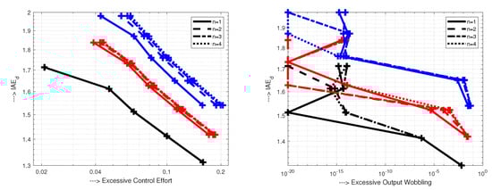
Improvements achieved for the same range of by augmenting PID to PIDA control filtered by (35) (Figure 11) are already not so remarkable as when extending PI to PID. SE and WE characteristics show that at the output, with the transients become 1P already for and at the input for . Thereby, they allow to achieve nearly ideal 1P transients at the input and output with lower IAE values. Again, the value in (82) guarantees ideal 1P shapes just at the output.
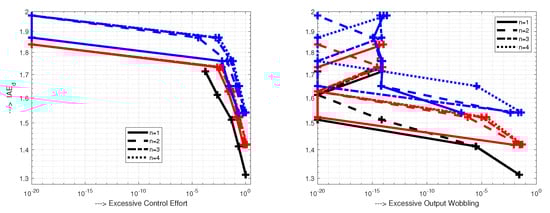
5.3. Example 3: SE and SW Characteristics—External Noise
The following example will illustrate the results given in [6], where it was shown that “smooth” (i.e., nearly 1P) input and output transients are achieved by slightly different values of than recommended in (8) or in (82) in Example 1. The tested controllers, filters and the optimal parameters are given below:
The results of the experiment (see SE and SW characteristics in Figure 12) show that by increasing the controllers order, the IAE values decrease without significant increase of the controller effort. Thus the results evidently refute general belief that controllers with a derivative action are not suitable for noisy systems. On the contrary, it is clearly shown that the closed-loop transients may be accelerated, with simultaneously decreasing the controller output noise, just by increasing the controller derivative order. In other words, when properly combining filtration, which yields smoother, but slightly slower transients, with derivative action (prediction) allowing faster, but noise amplifying dynamics, you may get faster responses without impairing their closed-loop shapes. Once upgrading PI to PID (as already done in [6]), we can continue with upgrading to PIDA, or to higher-order controllers (as used in the actual implementation of fractional order controllers, where the filters commonly exceed the order of 10)? During the era of pneumatic and other analog controllers, the PI control is used due to its simplicity [6]. However, as documented by increasing interest in fractional order PID, implemented by the HO controllers [2], the controller order does not play a role anymore in today’s software-implemented controllers. Taking into account that all the controllers are calculated from the same process model (in our case FOTD), it does not complicate process identification. Grimholt and Skogestad [6] are aware that with respect to the PI-tuning with , the iSIMC PID-tuning with improves IAE performance by about 30%, while keeping about the same robustness level (). Such PID controller is even better in almost all aspects than a well-tuned Smith Predictor. However, the HO controllers may also require solving problems associated with control constraints [19]. Moreover, frequent discard of the derivative term [1,16] may only be explained by improperly solved filtration problems. Here, it is important to mention that the differences between and in Figure 12 would be even more pronounced on extended x-. This means that the excessive control effort may be even lower by using at least 2nd order filters.
5.4. Example 4: SIMC and Newly Proposed Control of Fourth-Order System, No Noise
In [4], SIMC PI and PID control have also been applied to the fourth-order system (30) with and (33). By means of HR, this plant has either been approximated by FOTD model [4]
or by SOTD model
For , the FOTD model yields a SIMC PI (SPI) controller with
For , the SOTD model yields the SIMC PID controller (SPID) with parameters
On the other side, application of MHR yields the following models
The above models have been used in design of PI and PID controllers, PID and PIDA controllers and PIDA controller. In each case, we have chosen .
From the QOTD model (33) follows . However, zero value, and low values of , can lead to high controller gains causing oscillations. This can be avoided by taking into account the neglected time constants, which will eventually be translated into the effective dead-time value. These enable to replace the ideal with some positive number, chosen for example, as . In our case, with , the plant approximation used for the controller design is
Remark 5
(Reliability of model (33) in controller design). Although the addition of a transport delay to the model (33) may seem like a non-system solution, in reality, adhoc simplifications can be expected already in the process of obtaining (33). The assumption that the process has only a four-tuple dominant time constant and no other minor delays may correspond to reality only in very unlikely circumstances. Exact identification of shorter delays runs into numerical problems—in trying to identify exactly large dominant time constants, the determination of small delays in accuracy ceases. Nevertheless, if we could determine them, in the end, according to HR and MHR, we will still include them in . The problem can easily be demonstrated for example, when using Strejc identification [18]. There, the zero value of the transport delay is output only for specially measured process values, which we probably do not get on repeated identification. To obtain a model without a transport delay, the measured values must be rounded appropriately. Models based on such data manipulation may yield quite high data fitting in the identification evaluation. They can also give good results in controller design using reduced-order process models, when shorter time constants neglected are negligible compared to the dead-time resulting from model order reduction. However, they are not appropriate for a reliable controller design using models (30) with .
Figure 13 shows that for and , an increase of the derivative action order (e.g., from PI to PID, or from PID to PIDA) has virtually no effect on the process responses. However, the higher accuracy of the delay approximation, by using higher-order transfer functions and thus increasing the controller order, does not have a significant effect on the closed loop response in lag-dominant processes. The advantage of the newly proposed design is the possibility to significantly improve the control performance with simultaneously achieving nearly ideal shapes of process output transients.
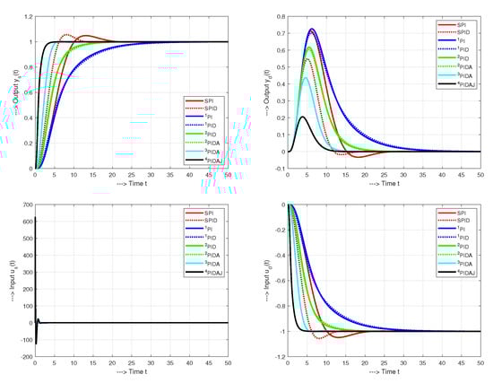
Figure 13.
Setpoint and input disturbance unit step responses of the system (33) by SPI, SPID, PI, PID, PID, PIDA, PIDA and PIDAJ controllers, no noise.
For all used controllers, the course of the control action at the setpoint change exhibits large signal swing. The initial control kick can be attenuated by using the derivative filter derived in Section 4. Another way to avoid derivative kick on setpoint change [4], is to follow industry practice by differentiating only the output of the system (or by using a setpoint weighting parameters). However, such a solution is not as efficient in terms of adapting the dynamics of the closed-loop responses when compared to pre-filters.
5.5. Example 5: Comparing SIMC PI and PID Controllers with the Newly Proposed Solutions Applied to Fourth-Order System
A comparison of the SIMC PI controller (SPI) and the newly designed PI controller in the above example implemented for shows faster SPI setpoint step response and slower, but strictly monotonic setpoint step response of PI control. However, such a comparison for a single tuning parameter value does not capture the resulting performance of the whole family of controllers. Figure 14 shows such responses corresponding to the plant approximations (85), (89) and the pre-filter (67) with the following values
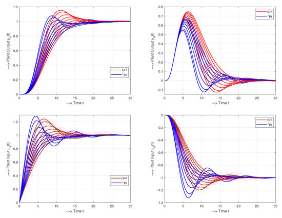
They illustrate that the nearly ideal shapes of the plant input and output signals, corresponding to the FOTD process model, are achieved at higher values than recommended in (8).
Thereby, the dynamics of the considered controllers depends on in different ways. The SE and SW characteristics in Figure 15 show that for the same values of shape-related deviations the IAE values of SPI controller are generally higher than for PI controller. For both controllers, increasing the decrease the excessive control effort and wobbling. However, the overshooting of the SPI controller, which indeed gives less IAE than for monotonic responses, is manifested by higher values of output wobbling and it does not fall to zero even for very high values of . From the results of comparison, it is clear that MHR gives better results than the HR when reducing higher order transfer functions for tuning the PI controllers.
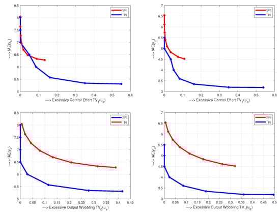
Figure 15.
SE and SW characteristics corresponding to transients with with SPI controller (red) in Figure 14 correspond mostly to higher IAE values than the transients with PI controller (blue), no noise.
Let us now discuss the details of the setpoint step responses of the PID controllers from Figure 13. The process (33) is represented by the second order models (86), or (90). Neglecting the initial peak, the process input is practically zero during the simulation time (Figure 16). Such kind of control cannot lead to robust closed-loop control. As decreases, this initial peak narrows and increases. Although the PID controller is much better in this respect than SPID, the initial peaks increase by decreasing . The problem can be solved by using pre-filters (68), or (78) derived in Section 4 and Section 4.2. In Figure 17, the transients of both compared controllers (SPID and PID) are shown for
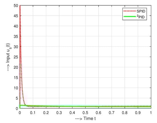
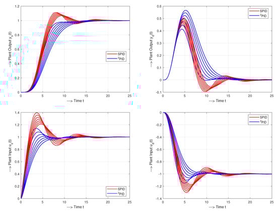
Obviously, the closed-loop responses are significantly faster when compared to the PI controllers in Figure 14. Thanks to the pre-filters used, their closed loop responses are smooth and without distinct peaks.
The SE and SW characteristics in Figure 18 show again that, by increasing , the IAE value changes much less for SPID controller and they are always above the values for PID controller for the same shape-related deviations. The PID controller results in zero shape-related deviations in almost the entire range of considered values. Again, it can be concluded that although processes with overshooting give less IAE than monotonic responses, the MHR gives, in combination with PID control, lower IAE values than the HR, when reducing the HO transfer function (33) order for the SPID controller design.
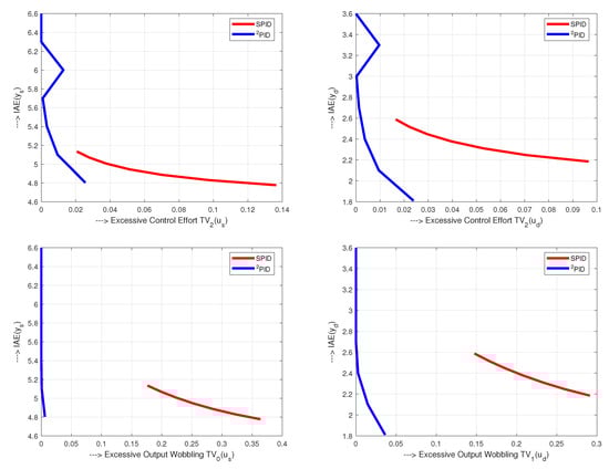
Figure 18.
SE and SW characteristics corresponding to transients in Figure 17 with SPID (red) and PID controllers (blue), no noise.
Remark 6
(Ambiguities of design and evaluation regarding the choice of pre-filter and ideal shape of ). The SE characteristics in Figure 18 evaluate the deviations from the ideal shape of the input signal using criterion. The criterion was chosen to unify the selection of controller and the evaluation of its performance. Similarly, when evaluating SPI and PI controllers in Figure 15, we calculated the deviations by using . However, the requirement for consistency of the controller design may lead to conclusion that we still control the fourth-order system (30), so we should use . Another possible proposal could require that we adapt the performance measures to the most complex controller used.
To illustrate broad spectrum of possible design alternations, the next comparison on the same example considers SPID controller (88) with pre-filter (78) and PIDA controller (28) based on the model (91) with a reduced-order pre-filter
Both control structures have been compared for the following tuning parameters:
To sufficiently suppress the measurement noise, a second-order filter has been used for SPID and a fourth-order filter for PIDA control, both with time constants , at the sampling period .
The closed-loop responses on unit step setpoint and disturbance unit step responses changes in Figure 19 show significantly faster dynamics of PIDA control compared to SPID control. The conclusions are also supported by the SE and SW characteristics in Figure 20. Given that SPID is based on the 2nd order model, we might expected ideal output shapes to be achieved with 2P input (i.e., transients from DC2) and use in the corresponding evaluation of the excessive control effort the measure. Using the same arguments for PIDA controller, the performance evaluation should work with . To illustrate the emerging differences, we will compare both performance measures.
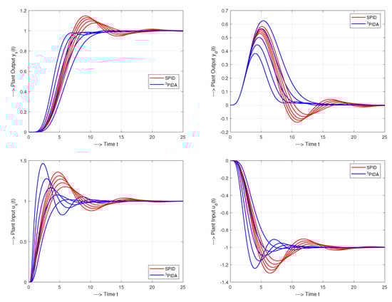
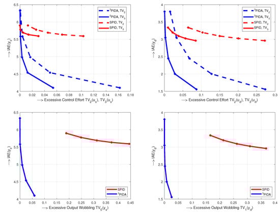
Figure 20.
SE and SW characteristics of SPID and PIDA controllers corresponding to transients in Figure 19.
The SE characteristics in Figure 20 demonstrate the difference between both measures. They show that, the process input, in terms of , when using the SPID controller, also provides ideal 3P responses for some larger values of the considered setting (96). However, the achievable range of IAE values is significantly narrower and the output signal deviations from the ideal responses are larger than with PIDA. Note that while with PIDA control, mainly affects the closed-loop speed without much effect on input and output shape deviations. On the other hand, with SPID, the correlation between the and the output shape is quite significant. At the same time, transients with PIDA control are both faster and smoother.
When using , the considered responses would give larger deviations than yielded by . From the comparison of numerical values in (45), it is then clear that the controller optimization based on prevents achieving the optimal performance, especially for the higher-order systems.
A similar conclusion is achieved when comparing the structure of SPID + with the PIDAJ controller proposed in Example 4 for the plant (92) and supplemented by the noise attenuation filter with and the reduced-order prefilter
In order to be able to speed up the loop responses under PIDAJ control, with respect to the PIDA controller, another value was added to the tuning parameter set (96):
Analysis of the family of time responses in Figure 21 yields the SE and SW characteristics in Figure 22.
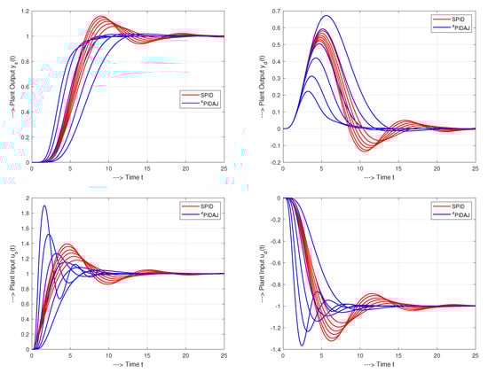
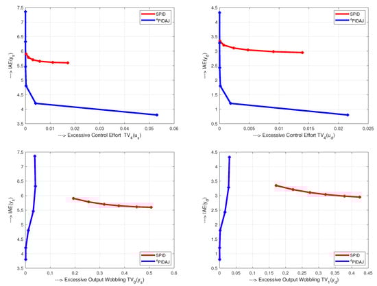
Figure 22.
SE and SW characteristics of SPID and PIDAJ controllers corresponding to transients in Figure 21.
The comparison with the characteristics in Figure 20 shows a significant decrease of values. The performance improvements for the PIDAJ controller, in terms of , are particularly visible in disturbance responses.
5.6. Example 6: SIMC and Newly Proposed Control of QOTD System with 3rd-Order Noise Attenuation Filters
The dynamics of the plant considered in the previous example will be evaluated with an external measurement noise with an amplitude generated in Matlab/Simulink by a Uniform Random Number block. To attenuate the noise impact, all considered controllers will be extended by the binomial filters (35) with the time constant . Based on the plant approximations and taking into account the filters using HR and MHR we get
Similar to the previous example, in order to obtain nearly ideal shapes of transients, SPI and PI controllers are tuned with . All other controllers are tuned with the default value of with pre-filters (69) except for SPID and PIDAJ, which use reduced-order pre-filters (99).
Since PID and PIDA controllers in Example 4 did not confirm any significant improvement over the PI and PID controllers, we are no longer considering them in this comparison.
The obtained transients in Figure 23 show that even under a relatively high measurement noise and higher-order derivative actions by some controllers, it is possible to significantly accelerate the responses while maintaining a relatively low control efforts. Here, it is worth noting that the lowest values of the excessive controller effort are not produced by the simplest controllers, despite the slow transients. However, when we look at the control signal responses in Figure 23 (associated with the nearly ideal responses of the output), we see that they are nearly monotonic. One pulse is visible in them only in case of setpoint response under PIDAJ with reduced-order pre-filter . Indications of 1P responses are also seen when using PID and PIDA controllers. Therefore, with respect to the Definition 5, these are the responses from DC0. In order for several pulses of the action variable to stand out more significantly (as discussed in Example 5), the level of measurement noise should be reduced.
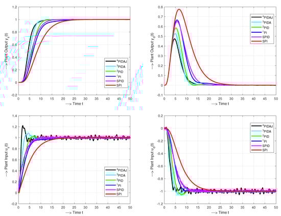
Figure 23.
Setpoint and input disturbance unit step responses of the system (33) for SPI, SPID, PI, PID, PIDA and PIDAJ controllers combined with the noise attenuation filters and tuning parameters for a measurement noise with an amplitude (i.e., up to 10% of the setpoint step) generated in Matlab/Simulink by a Uniform Random Number block.
Although the IAE values in Figure 24 (see also Table 1 and Table 2) decrease when using higher-order controllers, they do not show entire behavior of the responses, which should take into account both the speed of transients and excessive controller effort or output oscillation. From this point of view, the corresponding cost functions (50) and (51) show interesting results.
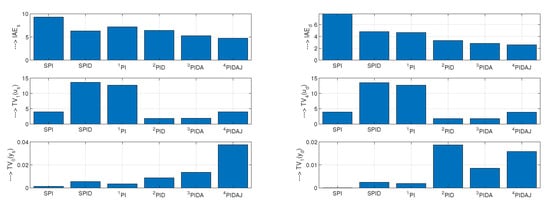
Figure 24.
Performance measures corresponding to transients in Figure 23.

Table 1.
Evaluation of the setpoint responses from Example 6.
Table 2.
Evaluation of the disturbance responses from Example 6.
Namely, for , when placing equal emphasis on the speed of transients and shape deviations, the optimal values of and are achieved with PIDA controller. By the same controller we get very good values also in terms of output wobbling . However, the best values of are obtained by the slowest SPI controller. On the other hand, when reflecting with increased demands on the speed of transients, the PIDAJ controller, resulting in the fastest transients for both setpoint and disturbance rejection responses, yields very good values also in terms of combined cost functions and .
6. Discussion: Everything Should Be Made as Simple as Possible, but Not Simpler
The discussion of the achieved results can be briefly summarized in a well-known statement attributed to Albert Einstein. The newly presented analytical design of HO-PID controllers and its comparison with SIMC and optimization-based iSIMC and other similar works leads us namely to the following comments—the published paper, “Probably the best simple PID tuning rules in the world” [43], was in fact mainly focused on “The best simple PI tuning rules”. Reference [4] was written in the same direction by suggesting adhoc choice in numerous points, as the choice of the target transfer function, half-rule for the reduction of complex plant models, or performance evaluation based on the IAE and TV. Later on, the SIMC author with the co-author analyzed the possibilities and limitations of the original method [44]. Recently, they have tried to extend the design to the PID controllers [6,22], where, they encountered the limitations of the initial postulates and tried to overcome them by using optimization methods. When trying to replace analytical approaches by the seemingly simpler numerical optimization approaches, we should note that:
- obtaining a perfect process model is frequently associated with trial-and-error approaches enabling to achieve the highest possible match between theoretical and experimentally obtained results (underpinned by appropriate identification results).
- These expectations are usually interpreted in terms of multicriteria cost functions, instead of a single general-purpose cost function and a single all-encompassing optimization.
- Diverse requirements led to the birth of fuzzy control based on the use of linguistically formulated conditions of optimality [45]. However, similar objectives can be easily achieved with simple analytical and modular approaches offering more direct relation to the tuning parameters, especially when they are designed to optimally cover the specific requirements.
- When looking for the optimal solution for a wider class of problems, the price to be paid is a wide range of existing and newly emerging controllers and methods for evaluating them. A simple list of existing solutions (as offered by [5]), with their ever-growing number, may not lead to a simplification and clarity of the situation. From this point of view, it seems more efficient to classify existing solutions into dynamic classes of control [17,39].
- From this perspective, the clear structure, openness, flexibility of adaptation and compatibility with the concept of dynamic classes can be considered as the main advantages of the newly proposed modifications to the original SIMC method.
It was found out that several of the proposed simplifications of the original SIMC were counterproductive or required certain modification. At the same time, as shown on the example of the system (33) taken from [4], there was identified the danger of exaggeration. Of course, simplifications are not avoided by the modified method. In order to suffice with the minimum possible number of parameters, it works with multiple time constants of the model already in the identification of the system, the choice of the target behavior, pre-filters and the choice of noise filters. By increasing the number of considered parameters, it would perhaps be possible to slightly improve the closed loop responses. However, the question is whether, in the face of all the existing uncertainties in real systems, it is worth it.
In the HO controller design and evaluation stages, it was essential to take into account the more complex shapes of transients. In addition to paying attention to the filter choice and limiting the main tuning parameter, this lead to design of pre-filters or setpoint weighting solutions. Our research led to final realization that, although based on SIMC, the core of its original concepts can be used on more complex controllers with higher order derivative actions.
7. Conclusions
This paper can be considered as an extension of the SIMC method to HO controllers with user-defined filter order. Although the paper focused on the stable process models, the SIMC method provided a versatile environment to satisfy challenging transient response requirements with some simple modifications. Noise attenuation requirements were met by choosing the filter order and time constant.
The key factor for the successful implementation of the HO controllers was appropriate signal filtering, since the higher-order derivatives without filters can be the main obstacle to practical implementation of the controller. The results of the illustrative examples showed that the proposed approach was suitable for implementation at different levels of process measurement noise.
The newly developed model-based approach for HO stable plants therefore provided excellent control results, which allow its implementation even in very demanding applications.
Author Contributions
Writing-original draft preparation, M.H. and D.V. Simulations, M.H. Editing, D.V. and M.H. Project administration, M.H. Both authors have read and agreed to the published version of the manuscript.
Funding
This research was funded by the grants APVV SK-IL-RD-18-0008 Platoon Modelling and Control for mixed autonomous and conventional vehicles: a laboratory experimental analysis, VEGA 1/0745/19 Control and modelling of mechatronic systems in emobility and P2-0001 financed by the Slovenian Research Agency.
Institutional Review Board Statement
Not applicable.
Informed Consent Statement
Not applicable.
Data Availability Statement
Not applicable.
Acknowledgments
Supported by Slovenská e-akadémia, n. o.
Conflicts of Interest
The authors declare no conflict of interest.
Abbreviations
The following abbreviations are used in this manuscript:
| 1P | One-Pulse, response with 2 monotonic segments (1 extreme point) |
| 2P | Two-Pulse, response with 3 monotonic segments (2 extreme points) |
| ART | Average Residence Time |
| BIBO | Bounded-Input-Bounded-Output |
| FOTD | First-Order Time Delayed |
| HO | Higher Order |
| HR | Half-Rule |
| I | Integrative |
| IMC | Internal Model Control |
| jOTD | j-Order Time Delayed |
| MHR | Modified Half-Rule |
| mP | m-Pulse, response with monotonic segments (m extreme points) |
| PI | Proportional-Integrative |
| PID | Proportional-Integrative-Derivative |
| PIDA | Proportional-Integrative-Derivative-Accelerative |
| PIDAJ | Proportional-Integrative-Derivative-Acceleration-Jerk |
| R | mth-order controller for jth-order stable plant, |
| R | mth-order controller for jth-order stable plant combined with nth-order filter , |
| SE | Speed - Effort |
| SIMC | Simple Control/Skogestad IMC |
| SPI | SIMC PI controller |
| SPID | SIMC PID controller |
| SW | Speed - Wobbling |
| SOTD | Second-Order Time Delayed |
| QOTD | Fourth-Order Time Delayed (with quadruple time constant) |
| TOTD | Third-Order Time Delayed |
References
- Åström, K.J.; Hägglund, T. Advanced PID Control; ISA, Research Triangle Park: Durham, NC, USA, 2006. [Google Scholar]
- Tepljakov, A.; Alagoz, B.B.; Yeroglu, C.; Gonzalez, E.; HosseinNia, S.H.; Petlenkov, E. FOPID Controllers and Their Industrial Applications: A Survey of Recent Results. IFAC-PapersOnLine 2018, 51, 25–30. [Google Scholar] [CrossRef]
- Efe, M.O. Fractional Order Systems in Industrial Automation: A Survey. IEEE Trans. Ind. Inform. 2011, 7, 582–591. [Google Scholar] [CrossRef]
- Skogestad, S. Simple analytic rules for model reduction and PID controller tuning. J. Process Control 2003, 13, 291–309. [Google Scholar] [CrossRef] [Green Version]
- O’Dwyer, A. Handbook of PI and PID Controller Tuning Rules, 3rd ed.; Imperial College Press: London, UK, 2009. [Google Scholar]
- Grimholt, C.; Skogestad, S. Optimal PI and PID control of first-order plus delay processes and evaluation of the original and improved SIMC rules. J. Process Control 2018, 70, 36–46. [Google Scholar] [CrossRef]
- Huba, M.; Vrančič, D.; Bisták, P. Control for IPDT Plants. Part 1: Disturbance Response. In Proceedings of the 26th Mediterranean Conference on Control and Automation (MED), Zadar, Croatia, 19–22 June 2018. [Google Scholar]
- Huba, M.; Vrančič, D. Comparing filtered PI, PID and PIDD2 control for the FOTD plants. In Proceedings of the 3rd IFAC Conference on Advances in Proportional-Integral-Derivative Control, Ghent, Belgium, 9–11 May 2018. [Google Scholar]
- Huba, M.; Vrančič, D. Introduction to the Discrete Time Control for the IPDT Plant. In Proceedings of the 15th IFAC International Conference on Programmable Devices and Embedded Systems, Ostrava, Czech Republic, 23–25 May 2018. [Google Scholar]
- Huba, M. Model-based higher-order PID control design. In Proceedings of the 21st IFAC World Congress, Berlin, Germany, 12–17 July 2020. [Google Scholar]
- Huba, M.; Vrančić, D.; Bisták, P. PID Control with Higher Order Derivative Degrees for IPDT Plant Models. IEEE Access 2021, 9, 2478–2495. [Google Scholar] [CrossRef]
- Skogestad, S. Tuning for Smooth PID Control with Acceptable Disturbance Rejection. Ind. Eng. Chem. Res. 2006, 45, 7817–7822. [Google Scholar] [CrossRef]
- Huba, M. Exploring PID tuning strategies considering noise impact in the IPDT plant control. In Proceedings of the 16th IFAC Int. Conference on Programmable Devices and Embedded Systems, High Tatras, Slovakia, 29–31 October 2019. [Google Scholar]
- Wei, Y.; Hu, Y.; Dai, Y.; Wang, Y. A Generalized Padé Approximation of Time Delay Operator. Int. J. Control. Autom. Syst. 2015, 14, 181–187. [Google Scholar] [CrossRef]
- Chien, K.L.; Hrones, J.; Reswick, J. On the automatic control of generalized passive systems. Trans. ASME 1952, 74, 175–185. [Google Scholar]
- Visioli, A. Practical PID Control; Springer: London, UK, 2006. [Google Scholar]
- Huba, M.; Šimunek, M. Modular Approach to Teaching PID Control. IEEE Trans. Ind. Electr. 2007, 54, 3112–3121. [Google Scholar] [CrossRef]
- Strejc, V. Näherungsverfahren für aperiodische Übergangscharakteristiken. Regelungstechnik 1959, 7, 124–128. [Google Scholar]
- Huba, M. Constrained filtered PID Controller for IPDT plants. In Proceedings of the 27th Mediterranean Conference on Control and Automation (MED), Akko, Israel, 1–4 July 2019. [Google Scholar]
- Segovia, V.R.; Hägglund, T.; Åström, K. Measurement noise filtering for PID controllers. J. Process Control 2014, 24, 299–313. [Google Scholar] [CrossRef]
- Rivera, D.E.; Morari, M.; Skogestad, S. Internal model control. 4. PID controller design. Ind Eng. Chem. Res. 1986, 25, 252–265. [Google Scholar] [CrossRef]
- Grimholt, C.; Skogestad, S. Optimal PID control of double integrating processes. IFAC-PapersOnLine 2016, 49, 127–132. [Google Scholar] [CrossRef]
- Åström, K.J.; Hägglund, T. PID Controllers: Theory, Design, and Tuning, 2nd ed.; Instrument Society of America: Research Triangle Park, NC, USA, 1995. [Google Scholar]
- Feldbaum, A. Optimal Control Systems; Academic Press: Cambridge, MA, USA, 1965. [Google Scholar]
- Pontrjagin, L.; Boltjanskij, V.; Gamkrelidze, R.; Miščenko, J. The Mathematical Theory of Optimal Processes; Interscience: New York, NY, USA, 1962. [Google Scholar]
- Föllinger, O. Regelungstechnik. 8. Auflage; Hüthig Buch Verlag: Heidelberg, Germany, 1994. [Google Scholar]
- Glattfelder, A.; Schaufelberger, W. Control Systems with Input and Output Constraints; Springer: Berlin, Germany, 2003. [Google Scholar]
- Huba, M. Designing Robust Controller Tuning for Dead Time Systems. In Int. Conf. System Structure and Control; IFAC: Ancona, Italy, 2010. [Google Scholar]
- Chen, W.H.; Yang, J.; Guo, L.; Li, S. Disturbance-Observer-Based Control and Related Methods – An Overview. IEEE Trans. Ind. Electron. 2016, 63, 1083–1095. [Google Scholar] [CrossRef] [Green Version]
- Huba, M. Performance measures, performance limits and optimal PI control for the IPDT plant. J. Process. Control. 2013, 23, 500–515. [Google Scholar] [CrossRef]
- Huba, M. Open flexible PD-controller design for different filtering properties. In Proceedings of the 39th Annual Conference of the IEEE Industrial Electronics Society (IECON), Vienna, Austria, 10–13 November 2013. [Google Scholar]
- Huba, M. Filter choice for an effective measurement noise attenuation in PI and PID controllers. In Proceedings of the ICM2015, Nagoya, Japan, 6–8 March 2015. [Google Scholar]
- Reswick, J.B. Disturbance-Response Feedback—A new control concept. Trans. ASME 1956, 1, 153–162. [Google Scholar]
- Huba, M.; Kulha, P.; Skachová, Z. Two Dynamical Classes of PI-Controllers for the 1st Order Loops. In Proceedings of the Preprints 2nd IFAC Workshop ”NTDCS” New Trends in Design of Control Systems, Smolenice, Slovak Republic, 7–10 September 1997; pp. 293–298.
- Hanus, R.; Peng, Y. Conditioning technique for controllers with time delays. IEEE Trans. Aututomatic Control 1992, 37, 689–692. [Google Scholar] [CrossRef]
- Kothare, M.; Campo, P.J.; Morari, M.; Nett, C.N. A Unified Framework for the Study of Anti-windup Designs. Automatica 1994, 30, 1869–1883. [Google Scholar] [CrossRef] [Green Version]
- Peng, Y.; Vrančič, D.; Hanus, R. Anti-Windup, Bumpless and Conditioned Trnasfer Techniques for PID Controllers. IEEE Control Syst. 1996, 16, 48–57. [Google Scholar]
- Peng, Y.; Vrančič, D.; Hanus, R. A Review of Anti-Windup, Bumpless and Conditioned Transfer. In Proceedings of the 13th IFAC World Congress, San Francisco, CA, USA, 30 June–5 July 1996; pp. 79–84. [Google Scholar]
- Huba, M.; Bistak, P. Dynamic classes in the PID control. In Proceedings of the 1999 American Control Conference (Cat. No. 99CH36251), San Diego, CA, USA, 2–4 June 1999; Volume 6, pp. 3868–3872. [Google Scholar]
- Huba, M. Constrained pole assignment control. In Current Trends in Nonlinear Systems and Control; Menini, L., Zaccarian, L., Abdallah, C.T., Eds.; Birkhäuser: Boston, MA, USA, 2006; pp. 163–183. [Google Scholar]
- Huba, M. Computer Design of Robust I-controller. In Proceedings of the IFAC World Congress, Milan, Italy, 28 August–2 September 2011; pp. 7468–7473. [Google Scholar]
- Huba, M. Robust Tuning of the Simplest Dead Time Compensators. In Proceedings of the 2014 International Conference and Exposition on Electrical and Power Engineering (EPE), Iasi, Romania, 16–18 October 2014. [Google Scholar]
- Skogestad, S. Probably the best simple PID tuning rules in the world. In Proceedings of the AIChE Annual Meeting, Reno, NV, USA, 4–9 November 2001. [Google Scholar]
- Grimholt, C.; Skogestad, S. Optimal PI-Control and Verifcation of the SIMC Tuning Rule. IFAC Proc. Vol. 2012, 45, 11–22. [Google Scholar] [CrossRef] [Green Version]
- Carvajal, J.; Chen, G.; Ogmen, H. Fuzzy PID controller: Design, performance evaluation, and stability analysis. Inf. Sci. 2000, 123, 249–270. [Google Scholar] [CrossRef]
Publisher’s Note: MDPI stays neutral with regard to jurisdictional claims in published maps and institutional affiliations. |
© 2021 by the authors. Licensee MDPI, Basel, Switzerland. This article is an open access article distributed under the terms and conditions of the Creative Commons Attribution (CC BY) license (https://creativecommons.org/licenses/by/4.0/).