Anderson Acceleration of the Arnoldi-Inout Method for Computing PageRank

Abstract

Anderson($m_0$) extrapolation, an accelerator to a fixed-point iteration, stores $m_0+1$ prior evaluations of the fixed-point iteration and computes a linear combination of those evaluations as a new iteration. The computational cost of the Anderson($m_0$) acceleration becomes expensive with the parameter $m_0$ increasing, thus $m_0$ is a common choice in most practice. In this paper, with the aim of improving the computations of PageRank problems, a new method was developed by applying Anderson(1) extrapolation at periodic intervals within the Arnoldi-Inout method. The new method is called the AIOA method. Convergence analysis of the AIOA method is discussed in detail. Numerical results on several PageRank problems are presented to illustrate the effectiveness of our proposed method.

1. Introduction

As the core technology of network information retrieval, Google’s PageRank model (called the PageRank problem) uses the original hyperlink structure of the World Wide Web to determine the importance of each page and has received a lot of attention in the last two decades. The core of the PageRank problem is to compute a dominant eigenvector (or PageRank vector) of the Google matrix $A$ by using the classical power method [1]:

$$Ax=x, A=\mathsf{\alpha }P+\left(1-\mathsf{\alpha }\right)v{e}^{\mathrm{T}}, \left|\right|x|{|}_1=1,$$

(1)

where $x$ is the PageRank vector, $e$ is a column vector with all elements equal to 1, $v$ is a personalized vector and the sum of its elements is 1, $P$ is a column-stochastic matrix (i.e., the dangling nodes have been replaced by columns with $1/n$), and $\alpha \in \left(0,1\right)$ is a damping factor.

As the damping factor $\alpha$ gradually approaches 1, the Google matrix is close to the original hyperlink structure. However, for large $\alpha$ such as $\alpha \ge 0.99$, the second eigenvalue ($\le \alpha$) of the matrix $A$ will be close to the main eigenvalue (equal to 1) [2], such that the classical power method suffers from slow convergence. In order to accelerate the power method, a lot of new algorithms are used to compute PageRank problems. The quadratic extrapolation method proposed by Kamvar et al. [3] accelerates the convergence by periodically subtracting estimates of non-dominant eigenvectors from the current iteration of the power method. It is worth mentioning that the authors [4] provide a theoretical justification for acceleration methods, generalizing the quadratic extrapolation and interpreting it as a Krylov subspace method. Gleich et al. [5] proposed an inner-outer iteration, wherein an inner PageRank linear system with a smaller damping factor is solved in each iteration. The inner-outer iteration shows good potential as a framework for accelerating PageRank computations, and a series of methods have been proposed based on it. For example, Gu et al. [6] constructed the power-inner-outer (PIO) method by combining the inner-outer iteration with the power method. It is worth mentioning that different versions of the Arnoldi algorithm applied to PageRank computations were first introduced in [7]. Gu and Wang [8] proposed the Arnoldi-Inout (AIO) algorithm by knitting the inner-outer iteration with the thick restarted Arnoldi algorithm [9]. Hu et al. [10] proposed a variant of the Power-Arnoldi (PA) algorithm [11] by using an extrapolation process based on a trace of the Google matrix $A$ [12].

Anderson($m_0$) acceleration [13,14] has been widely used to accelerate the convergence of a fixed-point iteration. Its principle is to store $m_0+1$ prior evaluations of the fixed-point method and compute a linear combination of those evaluations such that a new iteration is obtained. Anderson(0) is the given fixed-point iteration. Note that when the parameter $m_0$ becomes large, the computational cost of the Anderson($m_0$) acceleration becomes expensive. Hence, in most applications, $m_0$ is chosen to be small, and we set $m_0=1$ as a usual choice in this paper. In [15], Toth et al. proved that Anderson(1) extrapolation was locally q-linearly convergent. Pratapa et al. [16] developed the Alternating Anderson–Jacobi (AAJ) method by periodically employing Anderson extrapolation to accelerate the classical Jacobi iterative method for sparse linear systems.

In this paper, with the aim of accelerating the Arnoldi-Inout method for computing PageRank problems, the Anderson(1) extrapolation is used as an accelerator, and thus a new method is presented by combining the Anderson(1) extrapolation with the Arnoldi-Inout method periodically. Our proposed method is called the AIOA method, and its construction and convergence behavior are analyzed in detail, and numerical simulation experiments prove the effectiveness of the new algorithm.

The other parts of this article are structured as follows: In Section 2, we briefly review the Anderson acceleration and the Arnoldi-Inout method for PageRank problems. In Section 3, the AIOA method is constructed, and its convergence behavior is discussed. In Section 4, numerical comparisons are reported. Finally, in Section 5, we give some conclusions.

2. Previous Work

2.1. Anderson Acceleration

Anderson acceleration (also known as Anderson mixing) has been widely used in electronic structure computations [17]. Walker et al. [14] developed it for solving fixed-point problems: $x=g\left(x\right)$, where $x\in R^n$ and $\mathrm{g}:R^n\to R^n$. They showed that Anderson acceleration without truncation was essentially equivalent, in a certain sense, to the generalized minimum residual method (GMRES) [18] for linear problems. It has been proved that the Anderson iteration is convergent if the fixed-point iteration $g$ is a contraction and the coefficients in the linear combination remain bounded [15].

In this paper, we consider the Anderson(1) acceleration that stores two prior evaluations $g\left(x_0\right),g\left(x_1\right)$ and then computes $x_2$ (a linear combination of $g\left(x_0\right)$ and $g\left(x_1\right)$) as the new iteration. The main algorithmic steps of Anderson(1) are given as Algorithm 1.

Algorithm 1 The Anderson(1) acceleration
(1) Given an initial vector $x_0$.
(2) Compute $x_1=g\left(x_0\right)$, where $g$ is a fixed-point iteration.
(3) Compute $F=\left(f_0,f_1\right),$ where $f_i=g\left(x_i\right)-x_i,i=0,1$.
(4) Compute $\gamma ={\left({\gamma }_0,{\gamma }_1\right)}^{\mathrm{T}}$ that satisfies
$\underset{\gamma ={\left({\gamma }_0,{\gamma }_1\right)}^{\mathrm{T}}}{\min }||F\gamma |{|}_2,\hspace{1em}s.t.{{\displaystyle \sum }}_{i=0}^1{\gamma }_i=1.$	(2)
(5) Compute $x_2={\gamma }_{0}g\left(x_0\right)+\left(1-{\gamma }_0\right)g\left(x_1\right)$.

According to [15], the constrained linear least-squares problem (2) in step 4 of Algorithm 1 can be formulated as an equivalent, unconstrained least-squares problem:

$$\underset{ {\gamma }_0}{\min }||f_1+\left(f_0-f_1\right){\gamma }_0|{|}_2.$$

(3)

It is easy to solve the unconstrained least-squares problem$\left(3\right)$, for example, Pratapa et al. [16] chose the generalized inverse to compute ${\gamma }_0$, and Walker et al. [19] chose QR decomposition [18] to compute ${\gamma }_0$.

2.2. The Arnoldi-Inout Method for Computing PageRank

Gu and Wang [8] proposed the Arnoldi-Inout method by preconditioning the inner-outer iteration with the thick restarted Arnoldi method. Its algorithmic version can be found in Algorithm 2.

Algorithm 2 Arnoldi-Inout method [8]

Input: an initial vector $x_0$, the size of the subspace $m$, the number of approximate eigenvectors that are retained from one cycle to the next $\widehat{p}$, an inner tolerance $\eta$, an outer tolerance $\tau$, three parameters ${\alpha }_1,{\alpha }_2$, and $maxit$ to control the inner-outer iteration. Set $restart=0,r=1,d=1,d_0=d$.

Output: PageRank vector $x$.

(1). Apply the thick restarted Arnoldi algorithm [8,9] a few times (2–3 times). If the residual norm satisfies the prescribed tolerance, then stop; otherwise, continue.

(2). Run the inner-outer iteration with $x$ as the initial guess, where $x$ is the approximate vector obtained from the thick restarted Arnoldi algorithm:

$restart = 0$;

2.1. While $restart < maxit \& r > \tau$

2.2.            $x=x/\left|\right|x|{|}_1; z=Px;$

2.3.            $r=\left|\right|\alpha z+\left(1-\alpha \right)v-x|{|}_2;$

2.4.            $r_0=r; r_1=r; ratio=0;$

2.5.            While $ratio<{\alpha }_1 \& r> \tau$

2.6.                        $f=\left(\alpha -\beta \right)z+\left(1-\alpha \right)v;$

2.7.                        $rati{o}_1=0;$

2.8.                        While $rati{o}_1<{\alpha }_2 \& d> \eta$

2.9.                                    $x = f + \beta z; z = Px;$

2.10.                                  $d=\left|\right|f+\beta z-x|{|}_2;$

2.11.                                  $rati{o}_1=d/d_0;d_0=d;$

2.12.                        End While

2.13.                        $r=\left|\right|\alpha z+\left(1-\alpha \right)v-x|{|}_2;$

2.14.                        $ratio=r/r_0;r_0=r;$

2.15.            End While

2.16.            $x = \alpha z+\left(1-\alpha \right)v; x = x /\left|\right|x|{|}_1;$

2.17.            If$r/r_1>{\alpha }_1$

2.18.                        $restart = restart + 1;$

2.19.            End If

2.20. End While

2.21. If $r \le \tau$, stop, else goto step 1.

For Algorithm 2, it is necessary to indicate that:

(1)

The detailed description of the thick restarted Arnoldi algorithm in step 1 can be found in [8,9]. Here, we leave out its implementation for conciseness.

(2)

The parameters ${\alpha }_1,{\alpha }_2$,$restart$ and $maxit$ are used to control the conversion between the inner-outer iteration and the thick restarted Arnoldi algorithm. The specific utility mechanism and more details can be found in [8].

3. The AIOA Method for Computing PageRank

In this section, we combine the Arnoldi-Inout method with the Anderson(1) acceleration. The new method is called the AIOA method, which can be understood as the Arnoldi-Inout method accelerated with the Anderson(1) extrapolation. We first describe the construction of the AIOA method and then analyze its convergence behavior.

3.1. The Construction of the AIOA Method

The mechanism of the AIOA method can be described as follows: We first ran the Arnoldi-Inout method with a given initial guess $x_0$ to get an approximation vector ${\tilde{x}}_1$. If the approximation vector was unsatisfactory, then we treated the inner-outer iteration as a fixed-point problem and ran Algorithm 1 with vector ${\tilde{x}}_1$ as the starting vector to get another approximation vector $x_{new}$. If the vector $x_{new}$ did not work better than the approximation vector ${\tilde{x}}_3$ of the fixed-point problem, we set $x_{new}={\tilde{x}}_3$. If the new approximation vector $x_{new}$ was still not up to the specified accuracy, then we returned to the Arnoldi-Inout method with $x_{new}$ as the starting vector. We repeated the above process similarly until the required accuracy was reached. The specific algorithmic version is shown as follows.

3.2. Convergence Analysis

The convergence of the Arnoldi-Inout method and that of the Anderson acceleration can be found in [8,14,15]. In this subsection, we analyze the convergence of the AIOA method. Specifically, the convergence analysis of Algorithm 3 focuses on the process when turning from the Anderson(1) acceleration to the Arnoldi-Inout method.

Algorithm 3 AIOA method

(1). Given a unit initial guess $x_0$, an inner tolerance $\eta$, an outer tolerance $\tau$, the size of the subspace $m$, the number of approximate eigenvectors that are retained from one cycle to the next $\widehat{p}$, three parameters ${\alpha }_1,{\alpha }_2$ and $maxit$ to control the inner-outer iteration. Set $restart = 0, r = 1, d = 1, d_0 = d, l = 1$.

(2). Run the Algorithm 2 with the initial vector $x_0$. If the residual norm satisfies $\tau$, then stop, otherwise continue.

(3). Run the Algorithm 1 with ${\tilde{x}}_1$ as the starting guess, where ${\tilde{x}}_1$ is the approximation vector obtained from step 2.

3.1. $l=1,z=P{\tilde{x}}_1;$

3.2. While $l < 3 \& r > \tau$

3.3.               $f=\left(\alpha -\beta \right)z+\left(1-\alpha \right)v;$

3.4.               Repeat

3.5.                         $x = f + \beta z; z = Px;$

3.6.               Until $\left|\right|f+\beta z-x|{|}_2<\eta$

3.7.               $l = l + 1$;

3.8.               ${\tilde{x}}_{l } = \alpha z + \left(1 - \alpha \right)v;$

3.9.               $r=\left|\right|{\tilde{x}}_{l }-x|{|}_2;$

3.10. End While

3.11. Compute $f_0={\tilde{x}}_2-{\tilde{x}}_1, f_1={\tilde{x}}_3-{\tilde{x}}_2.$

3.12. Compute ${\gamma }_0$ that satisfies $\underset{{\gamma }_0}{\min }||f_1+\left(f_0-f_1\right){\gamma }_0|{|}_2$.

3.13. Compute $x_{new} = {\gamma }_0 {\tilde{x}}_2+ \left(1-{\gamma }_0\right) {\tilde{x}}_3$.

3.14. If $\left|\right|{\tilde{x}}_3-{\tilde{x}}_2|{|}_2<||x_{new}-{\tilde{x}}_2|{|}_2$

3.15.               $x_{new}= {\tilde{x}}_3;$

3.16. else

3.17.               $r=\left|\right|x_{new}-{\tilde{x}}_2|{|}_2;$

3.18. End If

3.19. If $r \le \tau$, stop, else go back to step 2 with the vector $x_{new}$ as the starting vector.

Let ${\mathcal{L}}_{m-1}$ denote the set of polynomials whose degree does not exceed $m-1$ and $\mathsf{\sigma }\left(A\right)$ represent the set of eigenvalues of the matrix $A$. Assume the eigenvalues of $A$ are sorted in the decreasing order $1=\left|{\lambda }_1\right|>\left|{\lambda }_2\right|\ge \cdots \ge \left|{\lambda }_n\right|$. The following theorem proposed by Saad [20] describes the relationship between an approximate eigenvector ${\mu }_1$ and the Krylov subspace ${\mathcal{K}}_m$.

Theorem 1.

[20] Assume that$A$is diagonalizable and that the initial vector$v_0$in Arnoldi’s method has expansion$v_0={{\displaystyle \sum }}_{i=1}^n{\zeta }_i{\mu }_i$with respect to the eigenbasis${\left\{{\mu }_i\right\}}_{i=1,2,3,\cdots ,n}$in which$\left|\right|{\mu }_i|{|}_1=1,i=1,2,3,\cdots ,n$and${\zeta }_1\ne 0$. Then the following inequality holds

$$\left|\right|\left(I-{\mathcal{P}}_m\right){\mu }_1|{|}_2\le \xi {\epsilon }_m,$$

(4)

where${\mathcal{P}}_m$is the orthogonal projector onto the subspace${\mathcal{K}}_m\left(A,v_0\right)$,$\xi ={{\displaystyle \sum }}_{i=2}^n\left|\frac{{\zeta }_i}{{\zeta }_1}\right|$and

$${\epsilon }_m=\underset{p\in {\mathcal{L}}_{m-1},p\left({\lambda }_1\right)=1}{\min }\underset{\lambda \in \sigma \left(A\right)/{\lambda }_1}{\max }\left|p\left(\lambda \right)\right|.$$

For the purpose of analyzing the convergence speed of our algorithm, it is given that two useful theorems about the spectrum properties of the Google matrix$A$ are as follows.

Theorem 2.

[21] Assume that the spectrum of the column-stochastic matrix$P$is$\left[1,{\pi }_2,\cdots ,{\pi }_n\right]$and then the spectrum of the matrix$A=\alpha P+\left(1-\alpha \right)e{v}^T$is$\left[1,\alpha {\pi }_2,\cdots ,\alpha {\pi }_n\right]$, where$\alpha \in \left(0,1\right),$and$v$is a vector with nonnegative elements such that$e^{T}v=1$.

Theorem 3.

[2] Let$P$be an$n \times n$column-stochastic matrix. Let$\alpha$be a real number such that$0 < \alpha < 1$. Let$E$be an$n \times n$rank-one column-stochastic matrix$E = v{e}^T$, where$e$is the$n$-vector whose elements are all ones and$v$is an$n$-vector whose elements are all nonnegative and sum to 1. Let$A=\alpha P+\left(1-\alpha \right)E$be an$n \times n$column-stochastic matrix, and then its dominant eigenvalue${\lambda }_1=1$,$\left|{\lambda }_2\right|\le \alpha$.

In the Arnoldi-Inout method, let $v_0$ from the previous thick restarted Arnoldi method be the starting vector for the inner-outer iteration. Next, the inner-outer method produces the vector $v_1=G^k{v}_0$, where $k \ge maxit$ and $G={\left(I-\beta P\right)}^{-1}\left[\left(\alpha -\beta \right)P+\left(1-\alpha \right)v{e}^{\mathrm{T}}\right]$. The derivation of the iterative matrix $G$ can be found in [5]. In our proposed method, we ran Algorithm 1 with vector$v_1$ as the initial vector. Note that in the Anderson(1) acceleration, we treated the inner-outer iteration as a fixed-point iteration such that the new vector $v_{new}=\omega \left[\left(1-{\gamma }_0\right)G^2{v}_1+{\gamma }_{0}G{v}_1\right]$ was produced such that $\mathsf{\omega }$ was the normalizing factor. If the vector $v_{new}$ worked better than the vector $G^2{v}_1$, then, as given in Algorithm 3, we set $v_{new}=G^2{v}_1$, which meant the Anderson(1) acceleration was reduced to the inner-outer iteration and the convergence of Algorithm 3 was certainly established for this case. Hence, it is discussed that the convergence for another case when the vector $v_{new}=\omega \left[\left(1-{\gamma }_0\right)G^2{v}_1+{\gamma }_{0}G{v}_1\right]$ works better than the vector$G^2{v}_1$.

In the next cycle of the AIOA algorithm, a $m$-step Arnoldi process was run with $v_{new}$ as the starting vector, and then the new Krylov subspace

$${\mathcal{K}}_m\left(A,v_{new}\right)=span\left(v_{new},A{v}_{new},\cdots ,A^{m-1}{v}_{new}\right)$$

was constructed. Next, we introduced the theorem that illustrates the convergence of the AIOA method.

Theorem 4.

Suppose that the matrix$A$is diagonalizable if we denote by$\widetilde{{\mathcal{P}}_m}$the orthogonal projector onto the subspace${\mathcal{K}}_m\left(A,v_{new}\right)$. Then under the notations of Theorem 1, it has

$$||\left(I-\widetilde{{\mathcal{P}}_m}\right){\mu }_1|{|}_2\le \Lambda ·{\left(\frac{\alpha -\beta }{1-\beta }\right)}^{k+1}·\xi {\epsilon }_m,$$

(5)

where$\Lambda =\left|\left(1-{\gamma }_0\right)\frac{\alpha -\beta }{1-\beta }+{\gamma }_0\right|$,$\xi ={{\displaystyle \sum }}_{i=2}^n\left|\frac{{\zeta }_i}{{\zeta }_1}\right|$,${\epsilon }_m=\underset{p\in {\mathcal{L}}_{m-1},p\left({\lambda }_1\right)=1}{\min }\underset{\lambda \in \sigma \left(A\right)/{\lambda }_1}{\max }\left|p\left(\lambda \right)\right|$and$k\ge maxit$.

Proof of Theorem 4.

For any$u \in {\mathcal{K}}_m\left(A,v_{new}\right)$, there exists $q\left(x\right)\in {\mathcal{L}}_{m-1}$ such that

$$\begin{array}{ll}u& =q\left(A\right)v_{new}\\ & =\omega ·q\left(A\right)·\left[\left(1-{\gamma }_0\right)G^2+{\gamma }_{0}G\right]v_1\\ & =\omega ·q\left(A\right)·\left[\left(1-{\gamma }_0\right)G^{k+2}+{\gamma }_0{G}^{k+1}\right]v_0\\ & =\omega ·q\left(A\right)·\left[\left(1-{\gamma }_0\right)G^{k+2}+{\gamma }_0{G}^{k+1}\right]·\left({\zeta }_1{\mu }_1+{\displaystyle \sum _{i=2}^n}{\zeta }_i{\mu }_i\right),\end{array}$$

(6)

where $v_0={{\displaystyle \sum }}_{i=1}^n{\mathsf{\zeta }}_i{\mu }_i$ is the expansion of $v_0$ within the eigenbasis $\left[{\mu }_1,{\mu }_2,\dots ,{\mu }_n\right]$.

As shown in [5] and [8], it has

$$\begin{array}{ll}G& ={\left(I-\beta P\right)}^{-1}\left[\left(\alpha -\beta \right)P+\left(1-\alpha \right)v{e}^{\mathrm{T}}\right]\\ & ={\left(I-\beta P\right)}^{-1}A-{\left(I-\beta P\right)}^{-1}+I,\end{array}$$

then

$$\begin{array}{ll}G{\mu }_i& ={\left(I-\beta P\right)}^{-1}A{\mu }_i - {\left(I-\beta P\right)}^{-1} {\mu }_i + {\mu }_i\\ & ={\left(I-\beta P\right)}^{-1}{\lambda }_i{\mu }_i-{\left(I-\beta P\right)}^{-1}{\mu }_i+{\mu }_i\\ & =\left({\lambda }_i-1\right){\left(I-\beta P\right)}^{-1}{\mu }_i+{\mu }_i,\end{array}$$

where we use$A{\mu }_i={\lambda }_i{\mu }_i, i = 1, 2, \dots , n$.

Assume that ${\pi }_i$ is an eigenvalue of $P$, and from Theorem 2, ${\pi }_1=1, {\pi }_i=\frac{1}{\mathsf{\alpha }}{\lambda }_i, i=2, 3, \dots , n$, then the matrix ${\left(I-\beta P\right)}^{-1}$ has eigenvalues

$${\eta }_i=\frac{1}{1-\beta {\pi }_i}, i=1,2,\dots ,n,$$

such that

$$G{\mu }_i=\frac{{\lambda }_i-\beta {\pi }_i}{1-\beta {\pi }_i}{\mu }_i, i=2,3,\dots ,n.$$

(7)

Using the fact that ${\lambda }_1=1$ and ${\pi }_1=1$, we have $G{\mu }_1={\mu }_1$ and $G^k{\mu }_1={\mu }_1$. Let

$${\phi }_i=\frac{{\lambda }_i-\beta {\pi }_i}{1-\beta {\pi }_i},i=2,3,\dots ,n,$$

then, according to Theorem 3 and derivation in [8], it has$\left|{\lambda }_i\right|\le \alpha , i = 2,3, \dots , n$, such that

$$\left|{\phi }_i\right|=\left|\frac{{\lambda }_i-\beta {\pi }_i}{1-\beta {\pi }_i}\right|\le \frac{\alpha -\beta }{1-\beta }.$$

(8)

Substituting (7) and (8) into (6), it has

$$u=\omega q\left(1\right){\zeta }_1{\mu }_1+\omega \left[\left(1-{\gamma }_0\right){\displaystyle \sum _{i=2}^n}q\left({\lambda }_i\right){\phi }_i^{k+2}{\zeta }_i{\mu }_i+{\gamma }_0{\displaystyle \sum _{i=2}^n}q\left({\lambda }_i\right){\phi }_i^{k+1}{\zeta }_i{\mu }_i\right],$$

and then

$$\begin{array}{ll}\left|\right|\frac{u}{\omega q\left(1\right){\zeta }_1}-{\mu }_1|{|}_2& =\left|\right|{{\displaystyle \sum }}_{i=2}^n\frac{{\zeta }_i}{{\zeta }_1}·\frac{q\left({\lambda }_i\right)}{q\left(1\right)}·{\phi }_i^{k+1}{\mu }_i·\left[\left(1-{\gamma }_0\right){\phi }_i+{\gamma }_0\right]|{|}_2\\ & \le \left|\left(1-{\gamma }_0\right)\frac{\alpha -\beta }{1-\beta }+{\gamma }_0\right|·{\left(\frac{\alpha -\beta }{1-\beta }\right)}^{k+1}{\displaystyle \sum _{i=2}^n}\left|\frac{{\zeta }_i}{{\zeta }_1}\right|·\underset{i\ne 1}{\max }\left|p\left({\lambda }_i\right)\right|\\ & =\Lambda ·{\left(\frac{\alpha -\beta }{1-\beta }\right)}^{k+1}\xi ·\underset{i\ne 1}{\max }\left|p\left({\lambda }_i\right)\right|,\end{array}$$

where we let $p\left(\mathsf{\lambda }\right)=q\left(\mathsf{\lambda }\right)/q\left(1\right)$ satisfy $p\left(1\right)=1$, $\xi ={{\displaystyle \sum }}_{i=2}^n\left|\frac{{\zeta }_i}{{\zeta }_1}\right|$ and $\Lambda =\left|\left(1-{\gamma }_0\right)\frac{\alpha -\beta }{1-\beta }+{\gamma }_0\right|$.

Therefore, we proved

$$\begin{array}{ll}||\left(I-\widetilde{{\mathcal{P}}_m}\right){\mu }_1|{|}_2& =\underset{u\in {\mathcal{K}}_m\left(A,v_{new}\right)}{\min }||u-{\mu }_1|{|}_2\\ & \le \Lambda ·{\left(\frac{\alpha -\beta }{1-\beta }\right)}^{k+1}·\xi ·\underset{p\in {\mathcal{L}}_{m-1},p\left({\lambda }_1\right)=1}{\min }\underset{\lambda \in \sigma \left(A\right)/{\lambda }_1}{\max }\left|p\left(\lambda \right)\right|.\end{array}$$

□

Remark 1.

Comparing (4) with (5), it is easy to find that our method can improve the convergence speed by a factor of at least$\Lambda ·{\left(\frac{\alpha -\beta }{1-\beta }\right)}^{k+1}$when turning from the Anderson(1) acceleration to the Arnoldi-Inout method.

4. Numerical Experiments

In this section, we first give the appropriate choice for the parameter $maxit$ and then test the effectiveness of the AIOA method. For the thick restarted Arnoldi method, there were two parameters, $m$ and $\widehat{p}$, that needed to be considered, but the thick restarted Arnoldi method had the same effect as the Arnoldi-Inout [8] method and the AIOA method. In addition, with the parameters $m$ and $\widehat{p}$ increasing, the cost would have been expensive, and they usually take small values. As a result, we don’t discuss the choice of the two parameters $m$ and $\widehat{p}$ in detail and set $m= 4$ and $\widehat{p}=3$ for all test examples.

All the numerical experiments were performed using MATLAB R2018a programming package on 2.10 GHZ CPU with 1 6GB RAM.

Table 1 lists the characteristics of the test matrices, where $n$ represents the matrix size, $nnz$ denotes the number of nonzero elements and $den$ is the density which is defined by $den=\frac{nnz}{n\times n}\times 100.$ All the test matrices are available from https://sparse.tamu.edu/ (accessed on 14 July 2020). For the sake of justice, the same initial guess $x_0=v=e/n$ with $e={\left[1,1,\cdots ,1\right]}^{\mathrm{T}}$ was used. The damping factors were chosen as $\alpha = 0.99, 0.993, 0.995$ and $0.998$ in all numerical experiments. The stopping criterion were set as the 2-norm of the residual, and the prescribed outer tolerance was $\tau ={10}^{-8}$. For the inner-outer iterations, the inner residual tolerance was $\eta ={10}^{-2}$, and the smaller damping factor was $\beta = 0.5$. The parameters chosen to control the flip-flop were ${\alpha }_1=\alpha -0.1$ and ${\alpha }_2=\alpha -0.1$. We ran the thick restarted Arnoldi procedure twice in each loop of the Arnoldi-Inout [8] method and the AIOA method. In the AIOA algorithm, we chose the QR decomposition to compute ${\gamma }_0$.

Table 1. The characteristics of test matrices.

Name	$\mathit{n}$	$\mathit{n}\mathit{n}\mathit{z}$	$\mathit{d}\mathit{e}\mathit{n}$
wb-cs-stanford	9914	36,854	$0.375\times {10}^{-1}$
usroads-48	126,146	323,900	$0.204\times {10}^{-2}$
web-Stanford	281,903	2,312,497	$0.291\times {10}^{-2}$
wiki-Talk	2,394,385	5,021,410	$0.875\times {10}^{-4}$

4.1. The Selection of Parameter $Maxit$

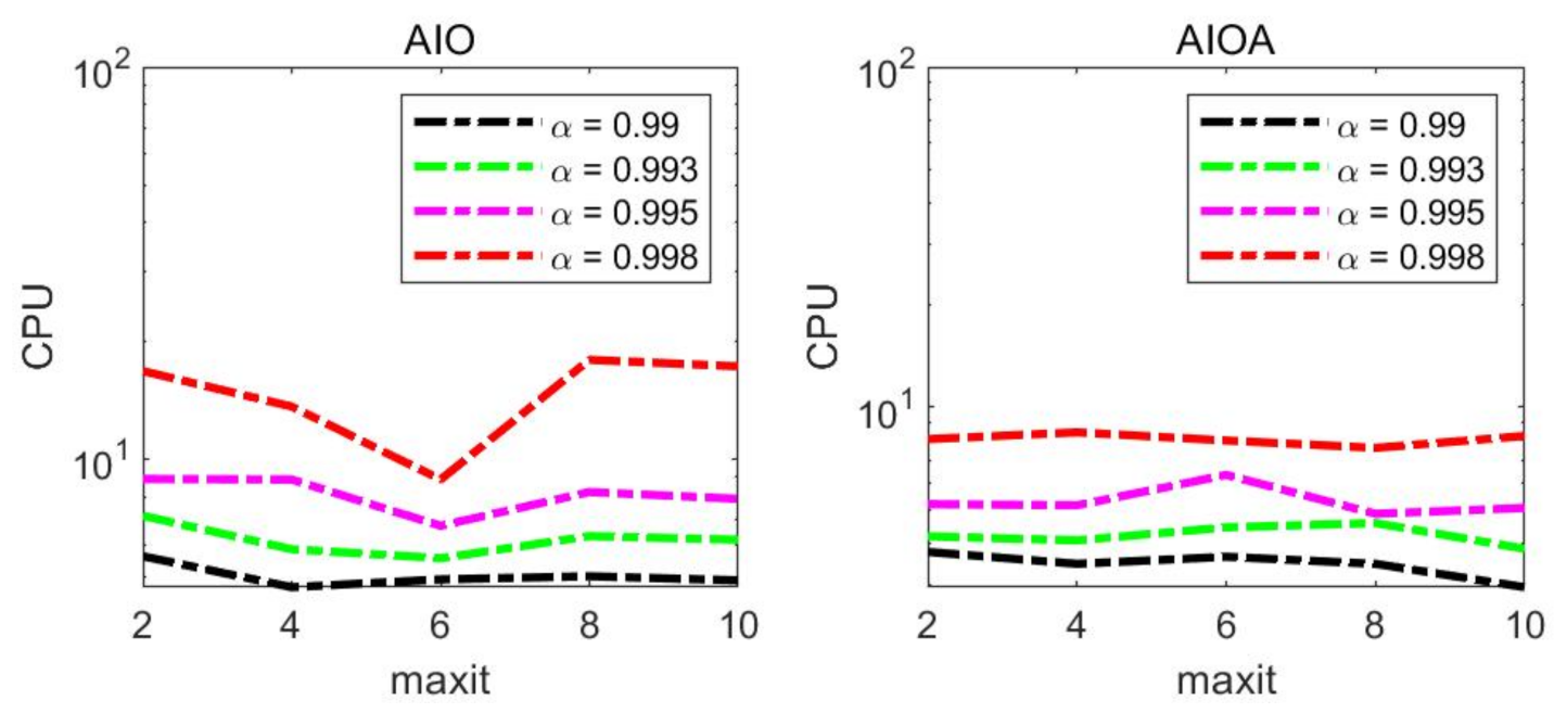
In this subsection, we discuss the selection of the parameter value $maxit$ by analyzing the numerical results of the Arnoldi-Inout [8] (denoted as “AIO”) method and the AIOA method for the web-Stanford matrix, which contains 281,903 pages and 2,312,497 links. Table 2 lists the matrix–vector products (MV) of the AIO method and the AIOA method for the web-Stanford matrix when $\alpha = 0.99, 0.993, 0.995, 0.998$ and $maxit = 2,4,6,8,10$. Figure 1 depicts the curves of computing time (CPU) of the two methods versus number $maxit$, respectively.

Table 2. The number of the matrix–vector products of the AIO method and the AIOA method on the web-Stanford matrix.

$\mathit{\alpha }$	$\mathit{m}\mathit{a}\mathit{x}\mathit{i}\mathit{t}=2$		$\mathit{m}\mathit{a}\mathit{x}\mathit{i}\mathit{t}=4$		$\mathit{m}\mathit{a}\mathit{x}\mathit{i}\mathit{t}=6$		$\mathit{m}\mathit{a}\mathit{x}\mathit{i}\mathit{t}=8$		$\mathit{m}\mathit{a}\mathit{x}\mathit{i}\mathit{t}=10$
	AIO	AIOA	AIO	AIOA	AIO	AIOA	AIO	AIOA	AIO	AIOA
$\alpha =0.99$	342	266	337	277	386	306	423	308	439	281
$\alpha =0.993$	446	309	422	327	433	376	542	417	563	358
$\alpha =0.995$	558	383	637	414	524	544	706	440	711	471
$\alpha =0.998$	1044	588	975	677	699	661	1503	669	1533	789

Figure 1. The total computing (CPU) time of the Arnoldi-Inout (AIO) method and the AIOA method versus number $maxit$ on the web-Stanford matrix.

From Table 2, it is observed that the optimal $maxit$ was different for different $\mathsf{\alpha }$ and different methods. From Figure 1, optimal $maxit$ is 6 and the worst performing $maxit$ is 8 for the AIO method, but for the AIOA method, the best value of $maxit$ is not 6. For fairness, we decided to choose the $maxit = 4$ in the following numerical experiments. In addition, in Table 2, when $\alpha = 0.995$ and $maxit = 6$, the MV of the AIOA is a little more than that of the AIO method, but the CPU time of AIOA method is better than that of the AIO method. The situation suggests that our method has some potential.

4.2. Comparisons of Numerical Results

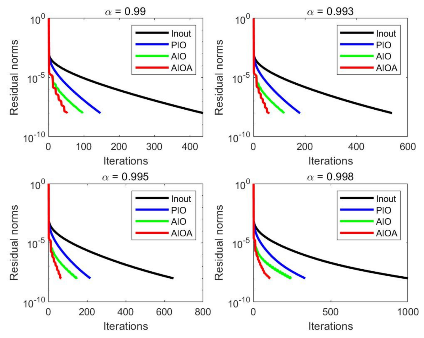
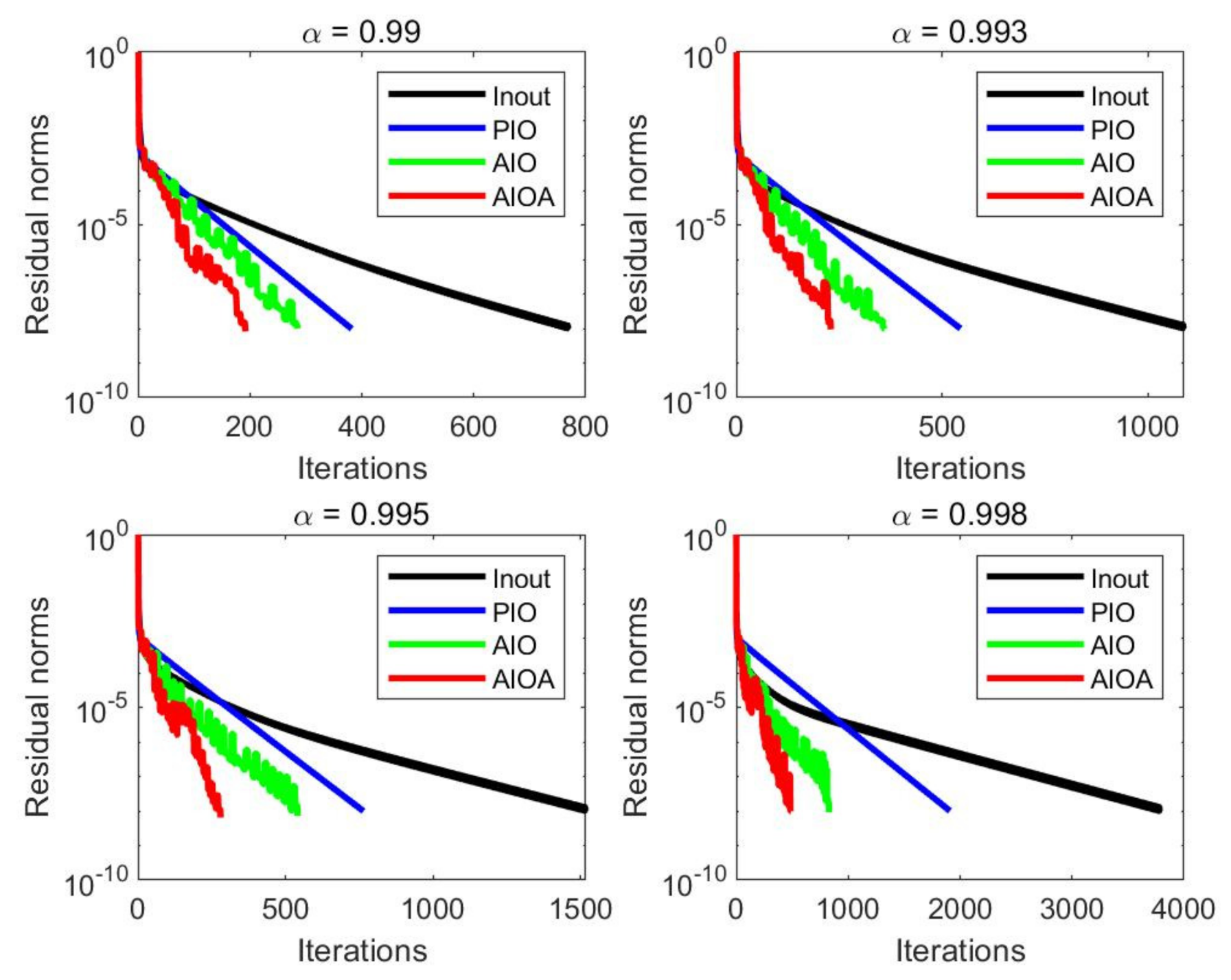
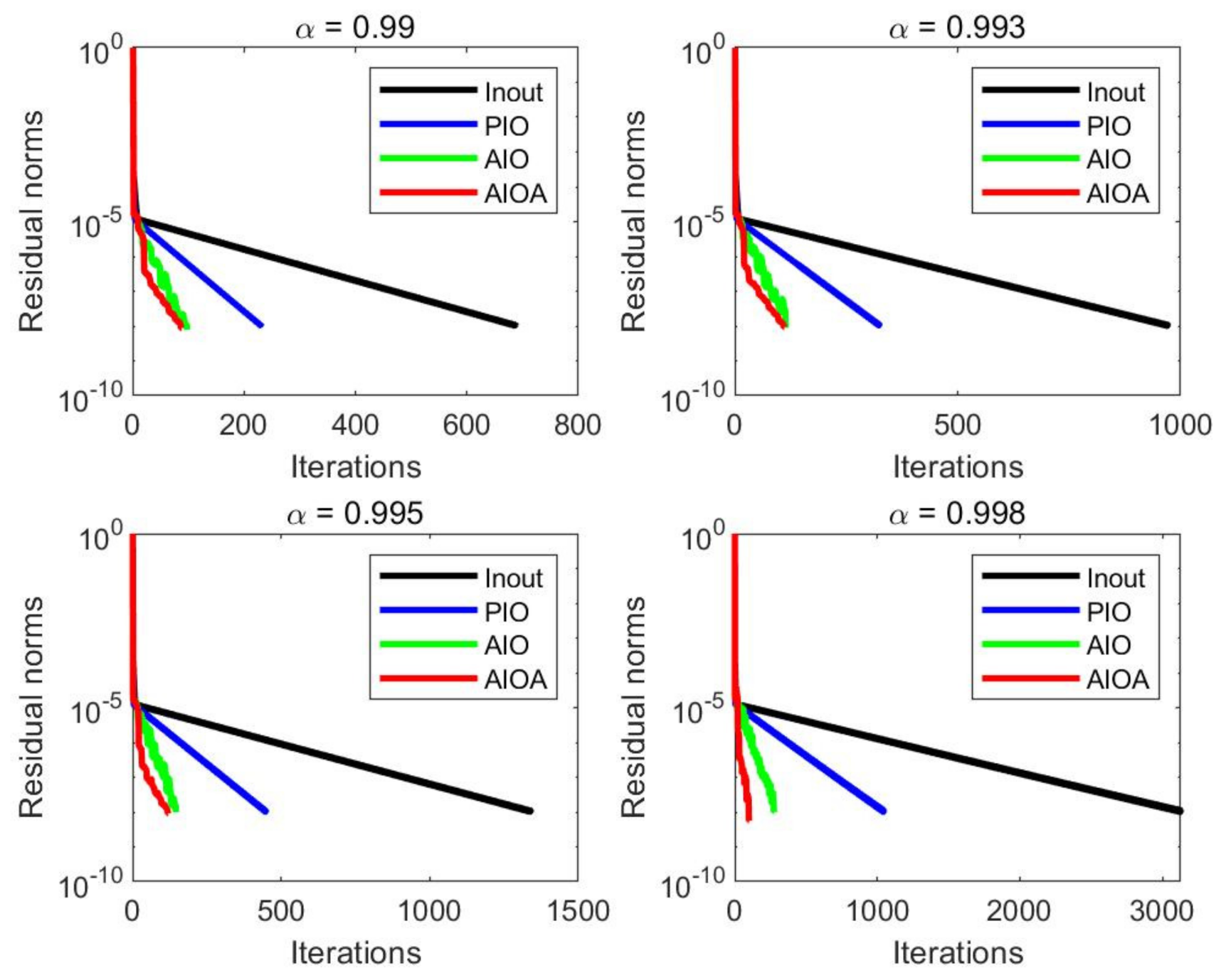
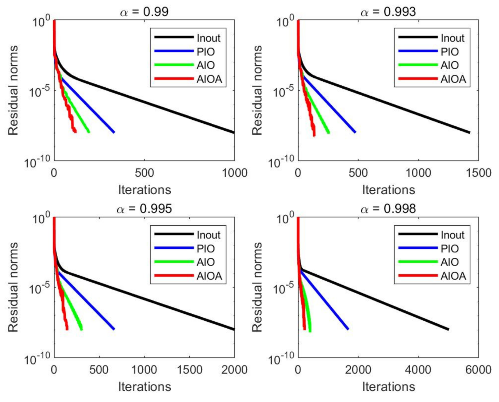
In this subsection, we tested the effectiveness of the AIOA method through numerical comparison experiments with the inner-outer (denoted as “Inout”) [5] method, the power-inner-outer (denoted as “PIO”) [6] method and the Arnoldi-Inout (denoted as “AIO”) [8] method in terms of iteration counts (IT), the number of matrix-vector products (MV) and the computing time (CPU) in seconds. In all experiments in this subsection, we set the parameters $m=4, \widehat{p}=3$ and $maxit = 4$. Table 3, Table 4, Table 5 and Table 6 give the numerical experiment results of the Inout method, the PIO method, the AIO method and the AIOA method for four matrices when $\alpha = 0.99, 0.993, 0.995, 0.998$, and Figure 2, Figure 3, Figure 4 and Figure 5 describe the residual convergence images of the above methods with different $\mathsf{\alpha }$ for all test matrices.

Table 3. Numerical results of the four methods on the wb-cs-stanford matrix.

$\mathit{\alpha }$		Inout	PIO	AIO	AIOA
$\alpha =0.99$	IT	997	333	192	116
	MV	997	666	238	167
	CPU	0.2344	0.2011	0.1741	0.1038
	speedup				40.35%
$\alpha =0.993$	IT	1427	476	252	133
	MV	1427	952	316	200
	CPU	0.3283	0.2488	0.2297	0.1211
	speedup				47.28%
$\alpha =0.995$	IT	2000	667	304	143
	MV	2000	1334	378	209
	CPU	0.4590	0.3490	0.2689	0.1273
	speedup				52.65%
$\alpha =0.998$	IT	5009	1670	396	216
	MV	5009	3340	496	315
	CPU	1.1347	0.8670	0.3817	0.1985
	speedup				47.99%

Table 4. Numerical results of the four methods on the usroads-48 matrix.

$\mathit{\alpha }$		Inout	PIO	AIO	AIOA
$\alpha =0.99$	IT	436	146	96	51
	MV	436	292	109	73
	CPU	1.1275	1.0362	0.7928	0.4347
	speedup				45.16%
$\alpha =0.993$	IT	537	180	118	59
	MV	537	360	135	84
	CPU	1.6484	1.0888	1.0487	0.6894
	speedup				34.26%
$\alpha =0.995$	IT	646	216	146	64
	MV	646	432	164	94
	CPU	1.9562	1.4969	1.1519	0.6894
	speedup				40.14%
$\alpha =0.998$	IT	999	334	242	106
	MV	999	668	272	155
	CPU	2.5375	2.0479	1.8138	0.9163
	speedup				49.48%

Table 5. Numerical results of the four methods on the web-Stanford matrix.

$\mathit{\alpha }$		Inout	PIO	AIO	AIOA
$\alpha =0.99$	IT	768	381	284	191
	MV	769	762	337	277
	CPU	9.5426	11.7488	8.4437	7.2447
	speedup				14.20%
$\alpha =0.993$	IT	1087	544	360	229
	MV	1088	1088	422	327
	CPU	10.4567	13.4826	11.0564	8.2018
	speedup				25.81%
$\alpha =0.995$	IT	1516	763	540	279
	MV	1517	1526	637	414
	CPU	16.6344	17.8678	17.0485	10.7983
	speedup				36.66%
$\alpha =0.998$	IT	3781	1908	828	484
	MV	3782	3816	975	677
	CPU	38.1507	43.2843	26.5169	16.8771
	speedup				36.35%

Table 6. Numerical results of the four methods on the wiki-Talk matrix.

$\mathit{\alpha }$		Inout	PIO	AIO	AIOA
$\alpha =0.99$	IT	687	230	97	86
	MV	687	460	117	109
	CPU	47.5235	34.3597	23.7834	20.1552
	speedup				15.25%
$\alpha =0.993$	IT	971	324	113	109
	MV	971	648	136	136
	CPU	73.2740	45.5463	27.8776	25.1927
	speedup				9.63%
$\alpha =0.995$	IT	1339	448	145	118
	MV	1339	896	173	157
	CPU	98.4781	62.3806	35.8122	29.3671
	speedup				17.99%
$\alpha =0.998$	IT	3127	1044	275	98
	MV	3127	2088	324	141
	CPU	208.5881	155.7358	65.6808	26.0576
	speedup				60.32%

Figure 2. Convergence behaviors of the four methods on the wb-cs-stanford matrix.

Figure 3. Convergence behaviors of the four methods on the usroads-48 matrix.

Figure 4. Convergence behaviors of the four methods on the web-Stanford matrix.

Figure 5. Convergence behaviors of the four methods on the wiki-Talk matrix.

In order to better demonstrate the efficiency of our proposed method, we defined

$$\mathit{speedup}=\frac{{\mathit{CPU}}_{\mathit{AIO}}-{\mathit{CPU}}_{\mathit{AIOA}}}{{\mathit{CPU}}_{\mathit{AIO}}}\times 100\%,$$

to show the speedup of the AIOA method with respect to the AIO method in terms of CPU.

From the numerical results in Table 3, Table 4, Table 5 and Table 6, it is easy to see that the AIOA method performed better than the other three methods in terms of IT, MV and CPU time for four matrices with different damping factors. As we expected, the advantage of the AIOA method was obvious for large $\mathsf{\alpha }$. For instance, when$\alpha = 0.995$, the speedup is $52.65\%$ in Table 3 and $36.66\%$ in Table 5. When $\alpha = 0.998$, the speedup is $49.48\%$ in Table 4 and $60.32\%$ in Table 6. In addition, from Figure 2, Figure 3, Figure 4 and Figure 5, it is easy to observe that the AIOA method can reach the accuracy requirement faster than the Inout method, the PIO method and the AIO method for all test examples. Therefore, the above results verify the effectiveness of the AIOA method.

5. Conclusions

In this paper, by employing the Anderson(1) extrapolation at periodic intervals within the Arnoldi-Inout method, we have presented a new method called the AIOA method to accelerate the computation speed of PageRank problems. Its implementation process and convergence theorem can be found in Section 3. Numerical simulation experiment results in Section 4 proved that the AIOA method was very efficient and converged faster compared to the inner-outer method, the power-inner-outer method and the Arnoldi-Inout method. However, there is still a lot of work to be further studied. For example, it is difficult to handle the best choices for parameters $m, \beta , maxit$.

References

1. Page, L.; Brin, S.; Motwani, R. The PageRank Citation Ranking: Bringing Order to the Web; Stanford InfoLab: Stanford, CA, USA, 1999. [Google Scholar]
2. Haveliwala, T.; Kamvar, S. The Second Eigenvalue of the Google Matrix; Stanford InfoLab: Stanford, CA, USA, 2003. [Google Scholar]
3. Kamvar, S.D.; Haveliwala, T.H.; Manning, C.D.; Golub, G.H. Extrapolation methods for accelerating PageRank computations. In Proceedings of the 12th International Conference on World Wide Web, Budapest, Hungary, 20–24 May 2003; pp. 261–270. [Google Scholar]
4. Brezinski, C.; Redivo-Zaglia, M. The PageRank vector: Properties, computation, approximation, and acceleration. SIAM J. Matrix Anal. Appl. 2006, 28, 551–575. [Google Scholar] [CrossRef]
5. Gleich, D.F.; Gray, A.P.; Greif, C. An inner-outer iteration for computing PageRank. SIAM J. Sci. Comput. 2010, 32, 349–371. [Google Scholar] [CrossRef]
6. Gu, C.Q.; Xie, F.; Zhang, K. A two-step matrix splitting iteration for computing PageRank. J. Comput. Appl. Math. 2015, 278, 19–28. [Google Scholar] [CrossRef]
7. Golub, G.H.; Greif, C. An Arnoldi-type algorithm for computing page rank. BIT 2006, 46, 759–771. [Google Scholar] [CrossRef]
8. Gu, C.Q.; Wang, W. An Arnoldi-Inout algorithm for computing PageRank problems. J. Comput. Appl. Math. 2017, 309, 219–229. [Google Scholar] [CrossRef]
9. Morgan, R.B.; Zeng, M. A harmonic restarted Arnoldi algorithm for calculating eigenvalues and determining multiplicity. Linear Algebra Appl. 2006, 415, 96–113. [Google Scholar] [CrossRef] [Green Version]
10. Hu, Q.Y.; Wen, C.; Huang, T.Z.; Shen, Z.L.; Gu, X.M. A variant of the Power–Arnoldi algorithm for computing PageRank. J. Comput. Appl. Math. 2021, 381, 113034. [Google Scholar] [CrossRef]
11. Wu, G.; Wei, Y. A Power—Arnoldi algorithm for computing PageRank. Numer. Linear Algebra Appl. 2007, 14, 521–546. [Google Scholar] [CrossRef]
12. Tan, X. A new extrapolation method for PageRank computations. J. Comput. Appl. Math. 2017, 313, 383–392. [Google Scholar] [CrossRef]
13. Anderson, D.G. Iterative procedures for nonlinear integral equations. JACM 1965, 12, 547–560. [Google Scholar] [CrossRef]
14. Walker, H.F.; Ni, P. Anderson acceleration for fixed-point iterations. SIAM J. Numer. Anal. 2011, 49, 1715–1735. [Google Scholar] [CrossRef] [Green Version]
15. Toth, A.; Kelley, C.T. Convergence analysis for Anderson acceleration. SIAM J. Numer. Anal. 2015, 53, 805–819. [Google Scholar] [CrossRef]
16. Pratapa, P.P.; Suryanarayana, P.; Pask, J.E. Anderson acceleration of the Jacobi iterative method: An efficient alternative to Krylov methods for large, sparse linear systems. J. Comput. Phys. 2016, 306, 43–54. [Google Scholar] [CrossRef] [Green Version]
17. Yang, C.; Meza, J.C.; Wang, L.W. A trust region direct constrained minimization algorithm for the kohn–sham equation. SIAM J. Sci. Comput. 2007, 29, 1854–1875. [Google Scholar] [CrossRef] [Green Version]
18. Allaire, G.; Kaber, S.M.; Trabelsi, K.; Allaire, G. Numerical Linear Algebra; Springer: New York, NY, USA, 2008. [Google Scholar]
19. Walker, H.F. Anderson Acceleration: Algorithms and Implementations; Report MS-6-15-50; WPI Math. Sciences Dept.: Worcester, MA, USA, 2011. [Google Scholar]
20. Saad, Y. Numerical Methods for Large Eigenvalue Problems; Manchester University Press: Manchester, UK, 1992. [Google Scholar]
21. Langville, A.; Meyer, C. Google’s PageRank and Beyond: The Science of the Search Engine Rankings; Princeton University Press: Princeton, NJ, USA, 2006. [Google Scholar]