The Cosmological OTOC: A New Proposal for Quantifying Auto-Correlated Random Non-Chaotic Primordial Fluctuations ^†

Abstract

The underlying physical concept of computing out-of-time-ordered correlation (OTOC) is a significant new tool within the framework of quantum field theory, which now-a-days is treated as a measure of random fluctuations. In this paper, by following the canonical quantization technique, we demonstrate a computational method to quantify the two different types of cosmological auto-correlated OTO functions during the epoch when the non-equilibrium features dominates in primordial cosmology. In this formulation, two distinct dynamical time scales are involved to define the quantum mechanical operators arising from the cosmological perturbation scenario. We have provided detailed explanation regarding the necessity of this new formalism to quantify any random events generated from quantum fluctuations in primordial cosmology. We have performed an elaborative computation for the two types of two-point and four-point auto-correlated OTO functions in terms of the cosmological perturbation field variables and its canonically conjugate momenta to quantify random auto-correlations in the non-equilibrium regime. For both of the cases, we found significantly distinguishable non-chaotic, but random, behaviour in the OTO auto-correlations, which was not pointed out before in this type of study. Finally, we have also demonstrated the classical limiting behaviour of the mentioned two types of auto-correlated OTOC functions from the thermally weighted phase-space averaged Poisson brackets, which we found to exactly match the large time limiting behaviour of the auto-correlations in the super-horizon regime of the cosmological scalar mode fluctuation.

Contents
1	Introduction	4
2	Formulation of Non-Chaotic Auto-Correlated OTO Functions in Primordial Cosmology	9
	2.1      Non-Chaotic Auto-Correlated OTO Functions . . . . . . . . . . . . . . . . . . . . . . . . . . . . . . . . . . . . . . . . . . . . . . . . . . . . . . . . . . . . . . . . . . . . . . . . . . . . . . . . . . . . . . . . . . . . . . . . . . . . . . . . . . . . . . . . . . . . . . .	9
	2.2      Eigenstate Representation of Non-Chaotic OTOC in Quantum Statistical Mechanics . . . . . . . . . . . . . . . . . . . . . . . . . . . . . . . . . . . . . . . . . . . . . . . . . . . . . . . . . . . . . . . . . . . . . . . . . . . . . . . . . . . . . . .	12
	2.3      Constructing Non-Chaotic OTOC in Cosmology . . . . . . . . . . . . . . . . . . . . . . . . . . . . . . . . . . . . . . . . . . . . . . . . . . . . . . . . . . . . . . . . . . . . . . . . . . . . . . . . . . . . . . . . . . . . . . . . . . . . . . . . . . . . . . . . . . . . .	21
	2.3.1      For Massless Scalar Field . . . . . . . . . . . . . . . . . . . . . . . . . . . . . . . . . . . . . . . . . . . . . . . . . . . . . . . . . . . . . . . . . . . . . . . . . . . . . . . . . . . . . . . . . . . . . . . . . . . . . . . . . . . . . . . . . . . . . . . . . . . . . . . . . .	22
	2.3.2      For Partially Massless Scalar Field . . . . . . . . . . . . . . . . . . . . . . . . . . . . . . . . . . . . . . . . . . . . . . . . . . . . . . . . . . . . . . . . . . . . . . . . . . . . . . . . . . . . . . . . . . . . . . . . . . . . . . . . . . . . . . . . . . . . . . . . . .	24
	2.3.3      For Partially Massless Scalar Field . . . . . . . . . . . . . . . . . . . . . . . . . . . . . . . . . . . . . . . . . . . . . . . . . . . . . . . . . . . . . . . . . . . . . . . . . . . . . . . . . . . . . . . . . . . . . . . . . . . . . . . . . . . . . . . . . . . . . . . . . .	25
3	Quantum Non-Chaotic Auto-Correlated OTO Amplitudes and OTOC in Primordial Cosmology	26
	3.1      Computational Strategy for Non-Chaotic Auto-Correlated OTO Functions . . . . . . . . . . . . . . . . . . . . . . . . . . . . . . . . . . . . . . . . . . . . . . . . . . . . . . . . . . . . . . . . . . . . . . . . . . . . . . . . . . . . . . . . . . . . . .	27
	3.2      Classical Mode Functions to Compute Non-Chaotic Auto-Correlated OTO Functions in Cosmology . . . . . . . . . . . . . . . . . . . . . . . . . . . . . . . . . . . . . . . . . . . . . . . . . . . . . . . . . . . . . . . . . . . . . . . . .	29
	3.3      Quantum Mode Function to Compute Non-Chaotic Auto-Correlated OTO Functions in Primordial Cosmology . . . . . . . . . . . . . . . . . . . . . . . . . . . . . . . . . . . . . . . . . . . . . . . . . . . . . . . . . . . . . . .	32
	3.4      Quantum Operators for Non-Chaotic Auto-Correlated OTO Functions . . . . . . . . . . . . . . . . . . . . . . . . . . . . . . . . . . . . . . . . . . . . . . . . . . . . . . . . . . . . . . . . . . . . . . . . . . . . . . . . . . . . . . . . . . . . . . . . . .	32
	3.5      Cosmological Two-Point and Four-Point “In-In” Non-Chaotic OTO Amplitudes . . . . . . . . . . . . . . . . . . . . . . . . . . . . . . . . . . . . . . . . . . . . . . . . . . . . . . . . . . . . . . . . . . . . . . . . . . . . . . . . . . . . . . . . . .	33
	3.5.1      Non-Chaotic Auto-Correlators in Primordial Cosmology . . . . . . . . . . . . . . . . . . . . . . . . . . . . . . . . . . . . . . . . . . . . . . . . . . . . . . . . . . . . . . . . . . . . . . . . . . . . . . . . . . . . . . . . . . . . . . . . . . . . . . .	33
	3.5.2      Fourier Space Representation of the Commutator Bracket: Application to Two-Point Non-Chaotic Auto-Correlated OTO Functions . . . . . . . . . . . . . . . . . . . . . . . . . . . . . . . . . . . . . . .	36
	3.5.3      Fourier Space Representation of Square of the Commutator Bracket: Application to Four-Point Non-Chaotic Auto-Correlated OTO Functions . . . . . . . . . . . . . . . . . . . . . . . . . . . . . .	38
	3.6      Thermal Partition Function in Primordial Cosmology: Quantum Version . . . . . . . . . . . . . . . . . . . . . . . . . . . . . . . . . . . . . . . . . . . . . . . . . . . . . . . . . . . . . . . . . . . . . . . . . . . . . . . . . . . . . . . . . . . . . . . .	40
	3.6.1      Initial Quantum State in Primordial Cosmology . . . . . . . . . . . . . . . . . . . . . . . . . . . . . . . . . . . . . . . . . . . . . . . . . . . . . . . . . . . . . . . . . . . . . . . . . . . . . . . . . . . . . . . . . . . . . . . . . . . . . . . . . . . . . .	40
	3.6.2      Quantum Partition Function in Terms of Rescaled Perturbation Field Variable in Primordial Cosmology . . . . . . . . . . . . . . . . . . . . . . . . . . . . . . . . . . . . . . . . . . . . . . . . . . . . . . . . . . . . . .	42
	3.6.3      Quantum Partition Function in Terms of the Cosmological Scalar Curvature Perturbation Field Variable in Primordial Cosmology . . . . . . . . . . . . . . . . . . . . . . . . . . . . . . . . . . . . . . . .	42
	3.7      Trace of Two-Point “In-In” Non-Chaotic Extension of OTO Amplitudes for Primordial Cosmology . . . . . . . . . . . . . . . . . . . . . . . . . . . . . . . . . . . . . . . . . . . . . . . . . . . . . . . . . . . . . . . . . . . . . . . . .	43
	3.8      New OTOCS from Regularised Two-Point “In-In” Non-Chaotic Auto-Correlated OTO Amplitudes: Rescaled Field Version . . . . . . . . . . . . . . . . . . . . . . . . . . . . . . . . . . . . . . . . . . . . . . . . . . . .	44
	3.9      New OTOCS from Regularised Two-Point “In-In” Non-Chaotic Auto-Correlated OTO Amplitudes: Curvature Perturbation Field Version . . . . . . . . . . . . . . . . . . . . . . . . . . . . . . . . . . . . . . .	46
	3.10    Trace of Four-Point “In-In” Non-Chaotic Auto-Correlated OTO Amplitude for Primordial Cosmology . . . . . . . . . . . . . . . . . . . . . . . . . . . . . . . . . . . . . . . . . . . . . . . . . . . . . . . . . . . . . . . . . . . . . .	50
	3.11    New OTOCs from Regularised Four-Point “In-In” Non-Chaotic Auto-Correlated OTO Amplitudes: Rescaled Field Version . . . . . . . . . . . . . . . . . . . . . . . . . . . . . . . . . . . . . . . . . . . . . . . . . . . .	51
	3.11.1      Without Normalisation . . . . . . . . . . . . . . . . . . . . . . . . . . . . . . . . . . . . . . . . . . . . . . . . . . . . . . . . . . . . . . . . . . . . . . . . . . . . . . . . . . . . . . . . . . . . . . . . . . . . . . . . . . . . . . . . . . . . . . . . . . . . . . . . . .	51
	3.11.2      With Normalisation . . . . . . . . . . . . . . . . . . . . . . . . . . . . . . . . . . . . . . . . . . . . . . . . . . . . . . . . . . . . . . . . . . . . . . . . . . . . . . . . . . . . . . . . . . . . . . . . . . . . . . . . . . . . . . . . . . . . . . . . . . . . . . . . . . . .	52
	3.12   New OTOCS from Regularised Four-Point “In-In” Non-Chaotic Auto-Correlated OTO Amplitudes: Curvature Perturbation Field Version . . . . . . . . . . . . . . . . . . . . . . . . . . . . . . . . . . . . . . . .	55
	3.12.1      Without Normalisation . . . . . . . . . . . . . . . . . . . . . . . . . . . . . . . . . . . . . . . . . . . . . . . . . . . . . . . . . . . . . . . . . . . . . . . . . . . . . . . . . . . . . . . . . . . . . . . . . . . . . . . . . . . . . . . . . . . . . . . . . . . . . . . . .	55
	3.12.2      With Normalisation . . . . . . . . . . . . . . . . . . . . . . . . . . . . . . . . . . . . . . . . . . . . . . . . . . . . . . . . . . . . . . . . . . . . . . . . . . . . . . . . . . . . . . . . . . . . . . . . . . . . . . . . . . . . . . . . . . . . . . . . . . . . . . . . . . . .	55
4	Numerical Analysis I: Interpretation of Two-Point Non-Chaotic Auto-Correlated OTO Functions	55
5	Numerical Analysis II: Interpretation of Four-Point Non-Chaotic Auto-Correlated OTO Functions	58
6	Classical Limit of Non-Chaotic Auto-Correlated OTO Amplitudes and OTOC in Primordial Cosmology	70
	6.1      Computational Strategy for Non-Chaotic Auto-Correlated OTO Functions in the Classical Limit . . . . . . . . . . . . . . . . . . . . . . . . . . . . . . . . . . . . . . . . . . . . . . . . . . . . . . . . . . . . . . . . . . . . . . . . . . .	70
	6.2      Classical Limit of Cosmological Two-Point “In-In” Non-Chaotic OTO Amplitudes . . . . . . . . . . . . . . . . . . . . . . . . . . . . . . . . . . . . . . . . . . . . . . . . . . . . . . . . . . . . . . . . . . . . . . . . . . . . . . . . . . . . . . .	71
	6.3      Classical Limit of Cosmological Four-Point “In-In” Non-Chaotic OTO Amplitudes . . . . . . . . . . . . . . . . . . . . . . . . . . . . . . . . . . . . . . . . . . . . . . . . . . . . . . . . . . . . . . . . . . . . . . . . . . . . . . . . . . . . . . .	72
	6.4      Cosmological Partition Function: Classical Version . . . . . . . . . . . . . . . . . . . . . . . . . . . . . . . . . . . . . . . . . . . . . . . . . . . . . . . . . . . . . . . . . . . . . . . . . . . . . . . . . . . . . . . . . . . . . . . . . . . . . . . . . . . . . . . . . .	74
	6.4.1      Classical Partition Function in Terms of Rescaled Field Variable . . . . . . . . . . . . . . . . . . . . . . . . . . . . . . . . . . . . . . . . . . . . . . . . . . . . . . . . . . . . . . . . . . . . . . . . . . . . . . . . . . . . . . . . . . . . . . . .	74
	6.4.2      Classical Partition Function in Terms of Curvature Perturbation Field Variable . . . . . . . . . . . . . . . . . . . . . . . . . . . . . . . . . . . . . . . . . . . . . . . . . . . . . . . . . . . . . . . . . . . . . . . . . . . . . . . . . . .	74
	6.5      Classical Limit of Cosmological Two-Point Non-Chaotic OTOC: Rescaled Field Version . . . . . . . . . . . . . . . . . . . . . . . . . . . . . . . . . . . . . . . . . . . . . . . . . . . . . . . . . . . . . . . . . . . . . . . . . . . . . . . . . .	75
	6.6      Classical Limit of Cosmological Two-Point Non-Chaotic OTOC: Curvature Perturbation Field Version . . . . . . . . . . . . . . . . . . . . . . . . . . . . . . . . . . . . . . . . . . . . . . . . . . . . . . . . . . . . . . . . . . . . .	77
	6.7      Classical Limit of Cosmological Four-Point Non-Chaotic OTOC: Rescaled Field Version . . . . . . . . . . . . . . . . . . . . . . . . . . . . . . . . . . . . . . . . . . . . . . . . . . . . . . . . . . . . . . . . . . . . . . . . . . . . . . . . . .	77
	6.7.1      Without Normalisation . . . . . . . . . . . . . . . . . . . . . . . . . . . . . . . . . . . . . . . . . . . . . . . . . . . . . . . . . . . . . . . . . . . . . . . . . . . . . . . . . . . . . . . . . . . . . . . . . . . . . . . . . . . . . . . . . . . . . . . . . . . . . . . . . . .	77
	6.7.2      With Normalisation . . . . . . . . . . . . . . . . . . . . . . . . . . . . . . . . . . . . . . . . . . . . . . . . . . . . . . . . . . . . . . . . . . . . . . . . . . . . . . . . . . . . . . . . . . . . . . . . . . . . . . . . . . . . . . . . . . . . . . . . . . . . . . . . . . . . .	80
	6.8      Classical Limit of Cosmological Four-Point Non-Chaotic OTOC: Curvature Perturbation Field Version . . . . . . . . . . . . . . . . . . . . . . . . . . . . . . . . . . . . . . . . . . . . . . . . . . . . . . . . . . . . . . . . . . . . . .	81
	6.8.1      Without Normalisation . . . . . . . . . . . . . . . . . . . . . . . . . . . . . . . . . . . . . . . . . . . . . . . . . . . . . . . . . . . . . . . . . . . . . . . . . . . . . . . . . . . . . . . . . . . . . . . . . . . . . . . . . . . . . . . . . . . . . . . . . . . . . . . . . .	81
	6.8.2      With Normalisation . . . . . . . . . . . . . . . . . . . . . . . . . . . . . . . . . . . . . . . . . . . . . . . . . . . . . . . . . . . . . . . . . . . . . . . . . . . . . . . . . . . . . . . . . . . . . . . . . . . . . . . . . . . . . . . . . . . . . . . . . . . . . . . . . . . . .	81
7	Summary and Outlook	82
A	Asymptotic Features of the Scalar Mode Functions in Cosmological Perturbation Theory	84
B	Quantum Two-Point OTO Amplitudes for Cosmology	86
	B.1      Definition of OTO Amplitude $\hat{\Delta }({\mathbf{K}}_1,{\mathbf{K}}_2;{\tau }_1,{\tau }_2)$ . . . . . . . . . . . . . . . . . . . . . . . . . . . . . . . . . . . . . . . . . . . . . . . . . . . . . . . . . . . . . . . . . . . . . . . . . . . . . . . . . . . . . . . . . . . . . . . . . . . . .	86
	B.2      Definition of OTO Amplitude $\hat{\Delta }({\mathbf{K}}_2,{\mathbf{K}}_2;{\tau }_1,{\tau }_2)$ . . . . . . . . . . . . . . . . . . . . . . . . . . . . . . . . . . . . . . . . . . . . . . . . . . . . . . . . . . . . . . . . . . . . . . . . . . . . . . . . . . . . . . . . . . . . . . . . . . . . . . . . . . . . . . . . . .	86
C	Quantum Four-Point OTO Amplitudes for Cosmology	87
	C.1      Definition of OTO Amplitude ${\widehat{\mathcal{T}}}_1^{\left(1\right)}({\mathbf{k}}_1,{\mathbf{k}}_2,{\mathbf{k}}_3,{\mathbf{k}}_4;{\tau }_1,{\tau }_2)$ and ${\widehat{\mathcal{T}}}_1^{\left(2\right)}({\mathbf{k}}_1,{\mathbf{k}}_2,{\mathbf{k}}_3,{\mathbf{k}}_4;{\tau }_1,{\tau }_2)$ . . . . . . . . . . . . . . . . . . . . . . . . . . . . . . . . . . . . . . . . . . . . . . . . . . . . . . . . . . . . . . . . . . . . . . . . . . .	87
	C.2       Definition of OTO Amplitude ${\widehat{\mathcal{T}}}_2^{\left(1\right)}({\mathbf{k}}_1,{\mathbf{k}}_2,{\mathbf{k}}_3,{\mathbf{k}}_4;{\tau }_1,{\tau }_2)$ and ${\widehat{\mathcal{T}}}_2^{\left(2\right)}({\mathbf{k}}_1,{\mathbf{k}}_2,{\mathbf{k}}_3,{\mathbf{k}}_4;{\tau }_1,{\tau }_2)$ . . . . . . . . . . . . . . . . . . . . . . . . . . . . . . . . . . . . . . . . . . . . . . . . . . . . . . . . . . . . . . . . . . . . . . . . . . .	89
	C.3      Definition of OTO Amplitude ${\widehat{\mathcal{T}}}_3^{\left(1\right)}({\mathbf{k}}_1,{\mathbf{k}}_2,{\mathbf{k}}_3,{\mathbf{k}}_4;{\tau }_1,{\tau }_2)$ and ${\widehat{\mathcal{T}}}_3^{\left(2\right)}({\mathbf{k}}_1,{\mathbf{k}}_2,{\mathbf{k}}_3,{\mathbf{k}}_4;{\tau }_1,{\tau }_2)$ . . . . . . . . . . . . . . . . . . . . . . . . . . . . . . . . . . . . . . . . . . . . . . . . . . . . . . . . . . . . . . . . . . . . . . . . . . .	91
	C.4      Definition of OTO Amplitude ${\widehat{\mathcal{T}}}_4^{\left(1\right)}({\mathbf{k}}_1,{\mathbf{k}}_2,{\mathbf{k}}_3,{\mathbf{k}}_4;{\tau }_1,{\tau }_2)$ and ${\widehat{\mathcal{T}}}_4^{\left(2\right)}({\mathbf{k}}_1,{\mathbf{k}}_2,{\mathbf{k}}_3,{\mathbf{k}}_4;{\tau }_1,{\tau }_2)$ . . . . . . . . . . . . . . . . . . . . . . . . . . . . . . . . . . . . . . . . . . . . . . . . . . . . . . . . . . . . . . . . . . . . . . . . . . .	92
D	Computation of Classical Limit of Four-Point “In-In” OTO Amplitudes for Cosmology	94
E	Computation of the Trace of the Two-Point Amplitude in OTOC	98
F	Computation of the Trace of the Four-Point Amplitude in OTOC	100
G	Computation of the Trace of the Four-Point Amplitude in OTOC	103
H	Time-Dependent Four-Point Amplitudes in OTOC	105
	H.1      Computation of ${\mathcal{I}}_1^{\left(l\right)}({\tau }_1,{\tau }_2)$ and ${\mathcal{I}}_1^{\left(2\right)}({\tau }_1,{\tau }_2)$ . . . . . . . . . . . . . . . . . . . . . . . . . . . . . . . . . . . . . . . . . . . . . . . . . . . . . . . . . . . . . . . . . . . . . . . . . . . . . . . . . . . . . . . . . . . . . . . . . . . . . . . . . . . . . . . . . . .	106
	H.2      Computation of ${\mathcal{I}}_2^{\left(l\right)}({\tau }_1,{\tau }_2)$ and ${\mathcal{I}}_2^{\left(2\right)}({\tau }_1,{\tau }_2)$ . . . . . . . . . . . . . . . . . . . . . . . . . . . . . . . . . . . . . . . . . . . . . . . . . . . . . . . . . . . . . . . . . . . . . . . . . . . . . . . . . . . . . . . . . . . . . . . . . . . . . . . . . . . . . . . . . . .	109
	H.3      Computation of ${\mathcal{I}}_3^{\left(l\right)}({\tau }_1,{\tau }_2)$ and ${\mathcal{I}}_3^{\left(2\right)}({\tau }_1,{\tau }_2)$ . . . . . . . . . . . . . . . . . . . . . . . . . . . . . . . . . . . . . . . . . . . . . . . . . . . . . . . . . . . . . . . . . . . . . . . . . . . . . . . . . . . . . . . . . . . . . . . . . . . . . . . . . . . . . . . . . . .	109
	H.4      Computation of ${\mathcal{I}}_4^{\left(l\right)}({\tau }_1,{\tau }_2)$ and ${\mathcal{I}}_4^{\left(2\right)}({\tau }_1,{\tau }_2)$ . . . . . . . . . . . . . . . . . . . . . . . . . . . . . . . . . . . . . . . . . . . . . . . . . . . . . . . . . . . . . . . . . . . . . . . . . . . . . . . . . . . . . . . . . . . . . . . . . . . . . . . . . . . . . . . . . . .	110
	H.5      Computation of ${\mathcal{I}}_5^{\left(l\right)}({\tau }_1,{\tau }_2)$ and ${\mathcal{I}}_5^{\left(2\right)}({\tau }_1,{\tau }_2)$ . . . . . . . . . . . . . . . . . . . . . . . . . . . . . . . . . . . . . . . . . . . . . . . . . . . . . . . . . . . . . . . . . . . . . . . . . . . . . . . . . . . . . . . . . . . . . . . . . . . . . . . . . . . . . . . . . . .	110
	H.6      Computation of ${\mathcal{I}}_6^{\left(l\right)}({\tau }_1,{\tau }_2)$ and ${\mathcal{I}}_6^{\left(2\right)}({\tau }_1,{\tau }_2)$ . . . . . . . . . . . . . . . . . . . . . . . . . . . . . . . . . . . . . . . . . . . . . . . . . . . . . . . . . . . . . . . . . . . . . . . . . . . . . . . . . . . . . . . . . . . . . . . . . . . . . . . . . . . . . . . . . . .	111
	H.7      Computation of ${\mathcal{I}}_7^{\left(l\right)}({\tau }_1,{\tau }_2)$ and ${\mathcal{I}}_7^{\left(2\right)}({\tau }_1,{\tau }_2)$ . . . . . . . . . . . . . . . . . . . . . . . . . . . . . . . . . . . . . . . . . . . . . . . . . . . . . . . . . . . . . . . . . . . . . . . . . . . . . . . . . . . . . . . . . . . . . . . . . . . . . . . . . . . . . . . . . . .	112
	H.8      Computation of ${\mathcal{I}}_8^{\left(l\right)}({\tau }_1,{\tau }_2)$ and ${\mathcal{I}}_8^{\left(2\right)}({\tau }_1,{\tau }_2)$. . . . . . . . . . . . . . . . . . . . . . . . . . . . . . . . . . . . . . . . . . . . . . . . . . . . . . . . . . . . . . . . . . . . . . . . . . . . . . . . . . . . . . . . . . . . . . . . . . . . . . . . . . . . . . . . . . .	112
	H.9      Computation of ${\mathcal{I}}_9^{\left(l\right)}({\tau }_1,{\tau }_2)$ and ${\mathcal{I}}_9^{\left(2\right)}({\tau }_1,{\tau }_2)$ . . . . . . . . . . . . . . . . . . . . . . . . . . . . . . . . . . . . . . . . . . . . . . . . . . . . . . . . . . . . . . . . . . . . . . . . . . . . . . . . . . . . . . . . . . . . . . . . . . . . . . . . . . . . . . . . . . .	113
I	Computation of the Normalisation Factor in Four-Point OTOC	114
	I.1      Normalisation Factor of Four-Point OTOC Computed from Rescaled Field Variable . . . . . . . . . . . . . . . . . . . . . . . . . . . . . . . . . . . . . . . . . . . . . . . . . . . . . . . . . . . . . . . . . . . . . . . . . . . . . . . . . . . . . .	114
	I.2      Normalisation Factor of Four-Point OTOC Computed from Curvature Perturbation Field Variable . . . . . . . . . . . . . . . . . . . . . . . . . . . . . . . . . . . . . . . . . . . . . . . . . . . . . . . . . . . . . . . . . . . . . . . . .	117
J	Computation of the Normalisation Factor in Classical Limit of Four-Point OTOC	119
	J.1      Normalisation Factor of the Classical Version of Four-Point OTOC Computed from Rescaled Field Variable . . . . . . . . . . . . . . . . . . . . . . . . . . . . . . . . . . . . . . . . . . . . . . . . . . . . . . . . . . . . . . . . .	119
	J.2      Normalisation Factor of the Classical Version of Four-Point OTOC Computed from Curvature Perturbation Field Variable . . . . . . . . . . . . . . . . . . . . . . . . . . . . . . . . . . . . . . . . . . . . . . . . . . . .	120
References		122

1. Introduction

The underlying physical concept of out-of-time ordered correlation (OTOC) functions [1,2,3,4,5,6,7,8,9] within the framework of quantum field theory is considered to be a very strong theoretical tool to describe random phenomena in the quantum regime, particularly the phenomena of quantum chaos. This concept was first introduced within the framework of superconductivity to explicitly compute the vertex correction factor of current in Reference [10]. For the last few years, in the various contexts of gravitational paradigm, this computational tool has been frequently used to describe various random-chaotic phenomena very successfully. One can physically interpret OTO functions as a quantum analogue of the usual classical sensitivity against very small random fluctuations in the initial conditions.

To describe this in a better way, let us consider two quantum operators in different time scales, $X_1\left(t_1\right)$, $X_1\left(t_2\right)$, its canonically conjugate momenta ${\mathsf{\Pi }}_{X_1}\left(t_1\right)$ and ${\mathsf{\Pi }}_{X_1}\left(t_2\right)$, and using these operators the auto-correlated OTOs are defined as:

$$\begin{gathered} \underline{\mathbf{Auto}-\mathbf{Correlated}{\mathbf{OTOC}}_{\mathbf{1}}} \\ \underline{\mathbf{Two}-\mathbf{point}\mathbf{function}:} \end{gathered}$$

$$\begin{array}{ccc}& & Y_1(t_1,t_2):\equiv -{\langle \left[X_1\left(t_1\right),X_1\left(t_2\right)\right]\rangle }_{\beta }=-\frac{1}{Z\left(t_1\right)}\mathrm{Tr}\left[exp\left(-\beta H\left(t_1\right)\right)\left[X_1\left(t_1\right),X_1\left(t_2\right)\right]\right],\hfill \end{array}$$

(1)

$\underline{\mathbf{Four}-\mathbf{point}\mathbf{function}:}$

$$\begin{array}{ccc}& & C_1(t_1,t_2):\equiv -{\langle {\left[X_1\left(t_1\right),X_1\left(t_2\right)\right]}^2\rangle }_{\beta }=-\frac{1}{Z\left(t_1\right)}\mathrm{Tr}\left[exp\left(-\beta H\left(t_1\right)\right){\left[X_1\left(t_1\right),X_1\left(t_2\right)\right]}^2\right],\hfill \end{array}$$

(2)

$$\begin{gathered} \underline{\mathbf{Auto}-\mathbf{Correlated}{\mathbf{OTOC}}_{\mathbf{2}}} \\ \underline{\mathbf{Two}-\mathbf{point}\mathbf{function}:} \end{gathered}$$

$$\begin{array}{ccc}& & Y_2(t_1,t_2):\equiv -{\langle \left[{\mathsf{\Pi }}_{X_1}\left(t_1\right),{\mathsf{\Pi }}_{X_1}\left(t_2\right)\right]\rangle }_{\beta }=-\frac{1}{Z\left(t_1\right)}\mathrm{Tr}\left[exp\left(-\beta H\left(t_1\right)\right)\left[{\mathsf{\Pi }}_{X_1}\left(t_1\right),{\mathsf{\Pi }}_{X_1}\left(t_2\right)\right]\right],\hfill \end{array}$$

(3)

$\underline{\mathbf{Four}-\mathbf{point}\mathbf{function}:}$

$$\begin{array}{ccc}& & C_2(t_1,t_2):\equiv -{\langle {\left[{\mathsf{\Pi }}_{X_1}\left(t_1\right),{\mathsf{\Pi }}_{X_1}\left(t_2\right)\right]}^2\rangle }_{\beta }=-\frac{1}{Z\left(t_1\right)}\mathrm{Tr}\left[exp\left(-\beta H\left(t_1\right)\right){\left[{\mathsf{\Pi }}_{X_1}\left(t_1\right),{\mathsf{\Pi }}_{X_1}\left(t_2\right)\right]}^2\right],\hfill \end{array}$$

(4)

where the quantum partition function at finite temperature can be expressed as:

$\underline{\mathbf{Quantum}\mathbf{Partition}\mathbf{function}:}$

$$\begin{array}{ccc}& & Z\left(t_1\right)=\mathrm{Tr}\left[exp\left(-\beta H\left(t_1\right)\right)\right]\mathrm{where}\beta =\frac{1}{T}\mathrm{with}{k}_B=1,\hslash =\frac{h}{2\pi }=1,\hfill \end{array}$$

(5)

where $H\left(t_1\right)$ is the Hamiltonian of the quantum system under consideration which is defined at the time scale $t_1$. Here in the quantum regime is the effect of perturbation by the quantum operators ${\mathsf{\Pi }}_{X_1}\left(t_1\right)$ and ${\mathsf{\Pi }}_{X_1}\left(t_2\right)$ on the measurement of the quantum operators $X_1\left(t_1\right)$ and $X_1\left(t_2\right)$ on later time scales. In this theoretical construction, we assume that the corresponding one-point functions trivially vanish for both of the operators

$\underline{\mathbf{One}-\mathbf{point}{\mathbf{function}}_{\mathbf{1}}:}$

$$\begin{array}{ccc}& & {\langle X_1\left(t_1\right)\rangle }_{\beta }=\frac{1}{Z\left(t_1\right)}\mathrm{Tr}\left[exp\left(-\beta H\left(t_1\right)\right)X_1\left(t_1\right)\right]=0,\hfill \end{array}$$

(6)

$$\begin{array}{ccc}& & {\langle X_1\left(t_2\right)\rangle }_{\beta }=\frac{1}{Z\left(t_2\right)}\mathrm{Tr}\left[exp\left(-\beta H\left(t_2\right)\right)X_1\left(t_2\right)\right]=0.\hfill \end{array}$$

(7)

$\underline{\mathbf{One}-\mathbf{point}{\mathbf{function}}_{\mathbf{2}}:}$

$$\begin{array}{ccc}& & {\langle {\mathsf{\Pi }}_{X_1}\left(t_1\right)\rangle }_{\beta }=\frac{1}{Z\left(t_1\right)}\mathrm{Tr}\left[exp\left(-\beta H\left(t_1\right)\right){\mathsf{\Pi }}_{X_1}\left(t_1\right)\right]=0.\hfill \end{array}$$

(8)

$$\begin{array}{ccc}& & {\langle {\mathsf{\Pi }}_{X_1}\left(t_2\right)\rangle }_{\beta }=\frac{1}{Z\left(t_2\right)}\mathrm{Tr}\left[exp\left(-\beta H\left(t_2\right)\right){\mathsf{\Pi }}_{X_1}\left(t_2\right)\right]=0.\hfill \end{array}$$

(9)

The huge applicability of OTOC as a strong theoretical probe of gravity dual theories in terms of AdS/CFT [11,12] has attracted a lot of attention recently in various works. Many such examples can be given that feature the importance of the OTO functions in AdS/CFT [11,12]. Particularly, the study of shock waves [13,14,15,16,17] in black hole physics is one of the remarkable examples, which can be understood by various types of geometries within the framework of AdS/CFT. In addition, it is important to note that this particular study finally led to maximum saturation bound on Lyapunov exponent in the quantum regime. In the gravitational paradigm, this bound is explained in terms of the well-known red shift factor which is defined near the black hole event horizon having a Hawking temperature. In this context, the Sachdev–Ye–Kitaev (SYK) model [18,19,20,21,22,23,24,25,26,27,28,29,30,31,32,33,34,35,36,37,38,39,40,41,42,43,44,45,46,47,48,49,50,51,52] is the most famous example which explains the quantum mechanical features of $0+1$ dimensional Majorana fermions having inherent infinitely long disorder. From the past understanding from various works, it is a very well known fact that any gravitational paradigm having their own CFT dual are described by the strongly coupled quantum field theories.

Now we will point towards an unusual application of computing auto-correlations of OTO functions within the framework of primordial cosmology, which we have proposed in Reference [53] to describe the cosmological cross-correlated OTO function. In primordial cosmology, the most significant quantities that we study are the N-point functions of the scalar-tensor metric fluctuations. Here we consider the Friedmann–Lemaître–Robertson–Walker (FLRW) spatially flat background metric to describe our homogeneous, isotropic and expanding observed universe. Using this metric, cosmological perturbation theory can be studied to explain the origin of the mentioned scalar-tensor fluctuations. These quantum fluctuations are very fundamental objects from which one can compute all N-point functions in primordial cosmology [54,55,56,57,58,59,60,61,62,63,64,65,66,67,68,69,70,71,72,73,74,75,76,77,78,79,80,81]. Additionally, these quantum fluctuations can be treated as a seed of cosmological perturbations to describe the formation of galaxy and cluster formation at present. These correlators are described in a same time scale as the late time scale of our universe and describe the equilibrium configuration.

Then one can immediately ask about the question regarding the possible options left to explore the physics of primordial quantum fluctuations from the studies of these mentioned correlators:

• First possibility:
  The first possibility is to include future observational aspects to verify various theoretical proposals in cosmology. These theoretical proposals are appended below:
  • Primordial gravitational waves and tensor-to-scalar ratio [79,82,83,84,85,86,87,88,89,90,91,92,93,94,95,96,97,98,99,100,101,102,103,104,105,106,107,108,109,110,111,112].
  • Primordial non-Gaussianity [54,55,56,57,58,59,60,61,62,63,64,65,66,67,68,69,70,71,72,73,74,75,76,77,78,79,80,81].
  • Spectral running and scale dependence in primordial power spectrum [86,102,113,114,115].
  • New consistency relations [85,87,90,116,117,118].
• Second possibility:
  The second possibility is probing of new physics by including significant features in primordial cosmology. This can be done by incorporating the concept of out-of-equilibrium in primordial cosmological quantum correlation functions. Before this work and previous work done by us in Reference [53], it was not at all mentioned in the corresponding literature how to compute and finally quantify the cosmological correlators at out-of-equilibrium. It is also not even clear to what exact quantity one needs to compute to give an estimation of these mentioned new correlators. After this work, we are hopeful that at least technically we have provided some correct estimations of these non-equilibrium quantum correlators within the framework of primordial cosmology. Now to connect with the real cosmological scenario, let us mention some aspects appearing in the timeline of our universe where one can implement the presented methodology:
  • stochastic particle production during inflation [53,119,120,121,122,123],
  • warm Inflationary framework [124,125,126],
  • reheating [127,128,129,130,131],
  • stochastic inflationary framework [132,133,134,135,136],
  • quantum quench [137,138,139,140,141,142,143,144,145,146,147,148] in cosmology.

In Figure 1, we show a schematic diagram representing the different roles of cosmological OTOC within the framework of primordial cosmology. Then, further in Figure 2, we show the diagrammatic representation of two-point and four-point time ordered auto-correlators for the momentum and field. Next, in Figure 3, we show the diagrammatic representation of two-point OTO auto-correlators for the momentum and field within the framework of primordial cosmology.

Finally, in Figure 4 and Figure 5, we show the diagrammatic representation of four-point OTO auto-correlators for the field and momentum within the framework of primordial cosmology. Now we mention the major highlights of our obtained results in this paper (Note: Except the small details presented for cosmological perturbation theory for scalar modes, the rest of the computations presented in this paper are completely new. We have presented the details in terms of the massless, partially massless and massive scalar fields, which are not commonly discussed in the cosmology text book literature. As a result of this, the partial details of the computations are provided in the text portion of the paper and the rest of the details are presented in the Appendices. We believe this will be helpful for general readers.):

• Highlight I:
  The computation method presented in this paper helps us to quantify the quantum auto-correlations within the framework of primordial cosmology with random fluctuations. In this article, we have computed the expressions for the two-point and four-point auto-correlated cosmological OTO functions in the quantum regime. These computed expressions are completely new and the detailed discussions will be helpful to understand the underlying physical problem that we have studied in this paper.
• Highlight II:
  We have additionally studied the classical limits of the two-point and four-point auto-correlated cosmological OTO functions in terms of the phase-space thermal weighted average of classical Poisson brackets. Most importantly, this computation will provide the non-standard random behaviour, which is perfectly consistent with the expectations from the present scenario. Last but not the least, this particular computation will be very helpful to understand the super-horizon classical limiting behaviour of the computed auto-correlated OTO functions.
• Highlight III:
  The late time behaviour of the four-point auto-correlated OTO functions helps us to study the equilibrium feature of the quantum correlations which we have computed from the scalar cosmological perturbations. Obviously the scalar cosmological perturbation and its related stuffs upto quantizing the Hamiltonian is very well known, but the rest of the computations in this context are completely new. For better understanding purposes, we have provided a small portion of the cosmological perturbation with scalar modes before starting the computation of two- and four-point auto-correlated OTO functions.
• Highlight IV:
  We have provided the detailed computation of the normalised version of the four-point auto-correlated cosmological OTO functions which we found that are completely independent of the choice of the time-dependent perturbation variable appearing in the cosmological perturbation theory. To justify this statement, we have used co-moving gauge for simplicity.

This paper is organized as follows:

• In Section 2, we discuss the formalism of computing the auto-correlated OTO functions in the context of primordial cosmology. This formalism is new, which we have highlighted in this paper.
• In Section 3, we provide the detailed derivation of quantum two-point and four-point auto-correlated OTO amplitudes and the related OTO function within the framework of primordial cosmology. This is the new calculation that we have provided in this paper.
• In Section 4 and Section 5, we present the numerical results from the quantum two-point and four-point auto-correlated OTO functions and also discuss about its physical interpretation. It is important to note that the numerical predictions obtained from the mentioned computations are also new and provide a new direction in the framework of primordial cosmology.
• In Section 6, we discuss the classical limit of the two-point and four-point OTO amplitudes and the related implications in cosmology. This is another new result we have provided in this paper which gives us a better understanding of the super-horizon classical limiting behaviour of the system under consideration.
• In Appendix A, Appendix B, Appendix C, Appendix D, Appendix E, Appendix F, Appendix G, Appendix H, Appendix I and Appendix J, we provide the details of the computations used in various sections of the paper. We believe this will help the general readers to understand the underlying physical problem that we have addressed in this paper.

2. Formulation of Non-Chaotic Auto-Correlated OTO Functions in Primordial Cosmology

2.1. Non-Chaotic Auto-Correlated OTO Functions

Let us consider two quantum mechanical operators X and Y which are defined at two different time scale, i.e., $X\left(t\right),X\left(\tau \right)$ and $Y\left(t\right),Y\left(\tau \right)$. Then we will extract the information regarding the non-chaotic but random quantum mechanical correlation functions using the prescription of OTOC. In this context, the non-chaotic OTOCs are defined in terms of these quantum operators as:

$$\begin{array}{ccc}& & \mathbf{2}-\mathbf{point}{\mathbf{OTOC}}_{\mathbf{1}}:Y_1(t,\tau ):=-{\langle \left[X\left(t\right),X\left(\tau \right)\right]\rangle }_{\beta },\hfill \end{array}$$

(10)

$$\begin{array}{ccc}& & \mathbf{2}-\mathbf{point}{\mathbf{OTOC}}_{\mathbf{2}}:Y_2(t,\tau ):=-{\langle \left[Y\left(t\right),Y\left(\tau \right)\right]\rangle }_{\beta },\hfill \end{array}$$

(11)

$$\begin{array}{ccc}& & \mathbf{4}-\mathbf{point}{\mathbf{OTOC}}_{\mathbf{1}}:C_1(t,\tau ):=-{\langle {\left[X\left(t\right),X\left(\tau \right)\right]}^2\rangle }_{\beta },\hfill \end{array}$$

(12)

$$\begin{array}{ccc}& & \mathbf{4}-\mathbf{point}{\mathbf{OTOC}}_{\mathbf{2}}:C_2(t,\tau ):=-{\langle {\left[Y\left(t\right),Y\left(\tau \right)\right]}^2\rangle }_{\beta },\hfill \end{array}$$

(13)

where the thermal average of any operator is defined as:

$$\begin{array}{c}\hfill \mathbf{Thermal}\mathbf{average}:{\langle A\left(t\right)\rangle }_{\beta }:=\frac{1}{Z}\mathrm{Tr}\left[exp(-\beta H)A\left(t\right)\right],\end{array}$$

(14)

where the partition function of the system is defined as:

$$\begin{array}{c}\hfill \mathbf{Partition}\mathbf{function}:Z=\mathrm{Tr}\left[exp(-\beta H)\right].\end{array}$$

(15)

Explicitly, in terms of thermal averaging one can further write:

$$\begin{array}{ccc}& & \mathbf{2}-\mathbf{point}{\mathbf{OTOC}}_{\mathbf{1}}:Y_1(t,\tau ):=-\frac{1}{Z}\mathrm{Tr}\left[exp(-\beta H)\left[X\left(t\right),X\left(\tau \right)\right]\right],\hfill \end{array}$$

(16)

$$\begin{array}{ccc}& & \mathbf{2}-\mathbf{point}{\mathbf{OTOC}}_{\mathbf{2}}:Y_2(t,\tau ):=-\frac{1}{Z}\mathrm{Tr}\left[exp(-\beta H)\left[Y\left(t\right),Y\left(\tau \right)\right]\right],\hfill \end{array}$$

(17)

$$\begin{array}{ccc}& & \mathbf{4}-\mathbf{point}{\mathbf{OTOC}}_{\mathbf{1}}:C_1(t,\tau ):=-\frac{1}{Z}\mathrm{Tr}\left[exp(-\beta H){\left[X\left(t\right),X\left(\tau \right)\right]}^2\right],\hfill \end{array}$$

(18)

$$\begin{array}{ccc}& & \mathbf{4}-\mathbf{point}{\mathbf{OTOC}}_{\mathbf{2}}:C_2(t,\tau ):=-\frac{1}{Z}\mathrm{Tr}\left[exp(-\beta H){\left[Y\left(t\right),Y\left(\tau \right)\right]}^2\right].\hfill \end{array}$$

(19)

One can further write these contributions in terms of the thermal density matrix as:

$$\begin{array}{ccc}& & \mathbf{2}-\mathbf{point}{\mathbf{OTOC}}_{\mathbf{1}}:Y_1(t,\tau ):=-\mathrm{Tr}\left[\rho \left[X\left(t\right),X\left(\tau \right)\right]\right],\hfill \end{array}$$

(20)

$$\begin{array}{ccc}& & \mathbf{2}-\mathbf{point}{\mathbf{OTOC}}_{\mathbf{2}}:Y_2(t,\tau ):=-\mathrm{Tr}\left[\rho \left[Y\left(t\right),Y\left(\tau \right)\right]\right],\hfill \end{array}$$

(21)

$$\begin{array}{ccc}& & \mathbf{4}-\mathbf{point}{\mathbf{OTOC}}_{\mathbf{1}}:C_1(t,\tau ):=-\mathrm{Tr}\left[\rho {\left[X\left(t\right),X\left(\tau \right)\right]}^2\right],\hfill \end{array}$$

(22)

$$\begin{array}{ccc}& & \mathbf{4}-\mathbf{point}{\mathbf{OTOC}}_{\mathbf{2}}:C_2(t,\tau ):=-\mathrm{Tr}\left[\rho {\left[Y\left(t\right),Y\left(\tau \right)\right]}^2\right],\hfill \end{array}$$

(23)

where in this context the thermal density matrix is defined as:

$$\begin{array}{c}\hfill \mathbf{Thermal}\mathbf{density}\mathbf{matrix}:\rho =\frac{1}{Z}\mathrm{Tr}\left[exp(-\beta H)\right].\end{array}$$

(24)

Now, in the large time limit, the thermal average of the following four-point function can be factorized as:

$$\begin{array}{ccc}\hfill {\langle X\left(\tau \right)X\left(t\right)X\left(t\right)X\left(\tau \right)\rangle }_{\beta }& =& \underset{\mathbf{2}-\mathbf{point}\mathbf{disconnected}}{\underbrace{{\langle X\left(\tau \right)X\left(\tau \right)\rangle }_{\beta }}}\underset{\mathbf{2}-\mathbf{point}\mathbf{disconnected}}{\underbrace{{\langle X\left(t\right)X\left(t\right)\rangle }_{\beta }}}+\underset{\mathbf{Sub}-\mathbf{leading}\mathbf{contribution}}{\underbrace{\mathcal{O}(exp(-(t+\tau )/t_d))}},\hfill \end{array}$$

(25)

$$\begin{array}{ccc}\hfill {\langle X\left(t\right)X\left(\tau \right)X\left(\tau \right)X\left(t\right)\rangle }_{\beta }& =& \underset{\mathbf{2}-\mathbf{point}\mathbf{disconnected}}{\underbrace{{\langle X\left(t\right)X\left(t\right)\rangle }_{\beta }}}\underset{\mathbf{2}-\mathbf{point}\mathbf{disconnected}}{\underbrace{{\langle X\left(\tau \right)X\left(\tau \right)\rangle }_{\beta }}}+\underset{\mathbf{Sub}-\mathbf{leading}\mathbf{contribution}}{\underbrace{\mathcal{O}(exp(-(t+\tau )/t_d))}},\hfill \end{array}$$

(26)

$$\begin{array}{ccc}\hfill {\langle Y\left(\tau \right)Y\left(t\right)Y\left(t\right)Y\left(\tau \right)\rangle }_{\beta }& =& \underset{\mathbf{2}-\mathbf{point}\mathbf{disconnected}}{\underbrace{{\langle Y\left(\tau \right)Y\left(\tau \right)\rangle }_{\beta }}}\underset{\mathbf{2}-\mathbf{point}\mathbf{disconnected}}{\underbrace{{\langle Y\left(t\right)Y\left(t\right)\rangle }_{\beta }}}+\underset{\mathbf{Sub}-\mathbf{leading}\mathbf{contribution}}{\underbrace{\mathcal{O}(exp(-(t+\tau )/t_d))}},\hfill \end{array}$$

(27)

$$\begin{array}{ccc}\hfill {\langle Y\left(t\right)Y\left(\tau \right)Y\left(\tau \right)Y\left(t\right)\rangle }_{\beta }& =& \underset{\mathbf{2}-\mathbf{point}\mathbf{disconnected}}{\underbrace{{\langle Y\left(t\right)Y\left(t\right)\rangle }_{\beta }}}\underset{\mathbf{2}-\mathbf{point}\mathbf{disconnected}}{\underbrace{{\langle Y\left(\tau \right)Y\left(\tau \right)\rangle }_{\beta }}}+\underset{\mathbf{Sub}-\mathbf{leading}\mathbf{contribution}}{\underbrace{\mathcal{O}(exp(-(t+\tau )/t_d))}},\hfill \end{array}$$

(28)

where the two-point disconnected thermal two-point correlators can be expressed as:

$$\begin{array}{ccc}& & \mathbf{2}-\mathbf{point}{\mathbf{correlator}}_{\mathbf{1}}:{\langle X\left(t\right)X\left(t\right)\rangle }_{\beta }=-\frac{1}{Z}\mathrm{Tr}\left[exp(-\beta H)X\left(t\right)X\left(t\right)\right],\hfill \end{array}$$

(29)

$$\begin{array}{ccc}& & \mathbf{2}-\mathbf{point}{\mathbf{correlator}}_{\mathbf{2}}:{\langle X\left(\tau \right)X\left(\tau \right)\rangle }_{\beta }=-\frac{1}{Z}\mathrm{Tr}\left[exp(-\beta H)X\left(\tau \right)X\left(\tau \right)\right],\hfill \end{array}$$

(30)

$$\begin{array}{ccc}& & \mathbf{2}-\mathbf{point}{\mathbf{correlator}}_{\mathbf{3}}:{\langle Y\left(t\right)Y\left(t\right)\rangle }_{\beta }=-\frac{1}{Z}\mathrm{Tr}\left[exp(-\beta H)Y\left(t\right)Y\left(t\right)\right],\hfill \end{array}$$

(31)

$$\begin{array}{ccc}& & \mathbf{2}-\mathbf{point}{\mathbf{correlator}}_{\mathbf{4}}:{\langle Y\left(\tau \right)Y\left(\tau \right)\rangle }_{\beta }=-\frac{1}{Z}\mathrm{Tr}\left[exp(-\beta H)Y\left(\tau \right)Y\left(\tau \right)\right],\hfill \end{array}$$

(32)

where the time scale $t_d$ is identified as the dissipation or equilibrium time scale, which is given by:

$$\begin{array}{c}\hfill \mathbf{Dissipation}/\mathbf{equilibrium}\mathbf{time}\mathbf{scale}:t_d\sim \beta =\frac{1}{T}\mathrm{with}{k}_B=1.\end{array}$$

(33)

Here, T is the equilibrium temperature of the quantum mechanical system under consideration. It is important to mention here that the above-mentioned four possible four-point thermal correlation functions can be factorized into the multiplication of two distinctive disconnected two-point contributions if one can wait for a large time scale. The factorization, along with the sub-leading decaying contribution, is actually expected from our basic understanding of quantum statistical field theory. When we give a response to a quantum system it goes to out-of-equilibrium phase and the corresponding correlation function in the quantum regime starts randomly fluctuating with respect to the evolutionary time scale. During this initial time scale when the initial response is provided in terms of the initial condition to the quantum system, it is not possible to factorize the present four possibilities of the four-point out-of-time ordered correlation (OTOC) functions. If we wait for a long enough time then it is expected that the quantum random fluctuations achieve the thermodynamic equilibrium. During this time scale, one can actually factorize these four possible four-point OTOCs in terms of the products of two disconnected two-point functions and the sub-leading contribution actually decay with respect to the very late time scale with a finite small saturation value. As a result, from this late time scale, $t_d$, which is identified to be dissipation time scale, will give the measure of the inverse temperature at thermodynamic equilibrium.

On the other hand, ${\langle {\left[X\left(t\right),X\left(\tau \right)\right]}^2\rangle }_{\beta }$ and ${\langle {\left[Y\left(t\right),Y\left(\tau \right)\right]}^2\rangle }_{\beta }$ can be expressed in the long time limit as:

$$\begin{array}{ccc}\hfill C_1(t,\tau )=-{\langle {\left[X\left(t\right),X\left(\tau \right)\right]}^2\rangle }_{\beta }& =& -{\langle X\left(t\right)X\left(\tau \right)X\left(t\right)X\left(\tau \right)\rangle }_{\beta }-{\langle X\left(\tau \right)X\left(t\right)X\left(\tau \right)X\left(t\right)\rangle }_{\beta }\hfill \\ & & +{\langle X\left(\tau \right)X\left(t\right)X\left(t\right)X\left(\tau \right)\rangle }_{\beta }+{\langle X\left(t\right)X\left(\tau \right)X\left(\tau \right)X\left(t\right)\rangle }_{\beta }\hfill \\ & =& 2\left\{{\langle X\left(t\right)X\left(t\right)\rangle }_{\beta }{\langle X\left(\tau \right)X\left(\tau \right)\rangle }_{\beta }-\Re \left[{\langle X\left(t\right)X\left(\tau \right)X\left(t\right)X\left(\tau \right)\rangle }_{\beta }\right]\right\}\hfill \\ & & -\mathcal{O}(exp(-(t+\tau )/t_d)),\hfill \end{array}$$

(34)

$$\begin{array}{ccc}\hfill C_2(t,\tau )=-{\langle {\left[Y\left(t\right),Y\left(\tau \right)\right]}^2\rangle }_{\beta }& =& -{\langle Y\left(t\right)Y\left(\tau \right)Y\left(t\right)Y\left(\tau \right)\rangle }_{\beta }-{\langle Y\left(\tau \right)Y\left(t\right)Y\left(\tau \right)Y\left(t\right)\rangle }_{\beta }\hfill \\ & & +{\langle Y\left(\tau \right)Y\left(t\right)Y\left(t\right)Y\left(\tau \right)\rangle }_{\beta }+{\langle Y\left(t\right)Y\left(\tau \right)Y\left(\tau \right)Y\left(t\right)\rangle }_{\beta }\hfill \\ & =& 2\left\{{\langle Y\left(t\right)Y\left(t\right)\rangle }_{\beta }{\langle Y\left(\tau \right)Y\left(\tau \right)\rangle }_{\beta }-\Re \left[{\langle Y\left(t\right)Y\left(\tau \right)Y\left(t\right)Y\left(\tau \right)\rangle }_{\beta }\right]\right\}\hfill \\ & & -\mathcal{O}(exp(-(t+\tau )/t_d)).\hfill \end{array}$$

(35)

Now using these results considering the large time equilibrium behaviour, one can further compute the expressions for the normalised OTOCs in the present context, which are given by:

$$\begin{array}{ccc}\hfill {\mathcal{C}}_1(t,\tau )=\frac{C_1(t,\tau )}{{\langle X\left(t\right)X\left(t\right)\rangle }_{\beta }{\langle X\left(\tau \right)X\left(\tau \right)\rangle }_{\beta }}& =& \underset{\mathbf{Leading}\mathbf{contribution}}{\underbrace{2\left\{1-\frac{\Re \left[{\langle X\left(t\right)X\left(\tau \right)X\left(t\right)X\left(\tau \right)\rangle }_{\beta }\right]}{{\langle X\left(t\right)X\left(t\right)\rangle }_{\beta }{\langle X\left(\tau \right)X\left(\tau \right)\rangle }_{\beta }}\right\}}}\hfill \\ & & -\underset{\mathbf{Sub}-\mathbf{leading}\mathbf{decaying}\mathbf{contribution}}{\underbrace{\frac{\mathcal{O}(exp(-(t+\tau )/t_d))}{{\langle X\left(t\right)X\left(t\right)\rangle }_{\beta }{\langle X\left(\tau \right)X\left(\tau \right)\rangle }_{\beta }}}},\hfill \end{array}$$

(36)

$$\begin{array}{ccc}\hfill {\mathcal{C}}_1(t,\tau )=\frac{C_2(t,\tau )}{{\langle Y\left(t\right)Y\left(t\right)\rangle }_{\beta }{\langle Y\left(\tau \right)Y\left(\tau \right)\rangle }_{\beta }}& =& \underset{\mathbf{Leading}\mathbf{contribution}}{\underbrace{2\left\{1-\frac{\Re \left[{\langle Y\left(t\right)Y\left(\tau \right)Y\left(t\right)Y\left(\tau \right)\rangle }_{\beta }\right]}{{\langle Y\left(t\right)Y\left(t\right)\rangle }_{\beta }{\langle Y\left(\tau \right)Y\left(\tau \right)\rangle }_{\beta }}\right\}}}\hfill \\ & & -\underset{\mathbf{Sub}-\mathbf{leading}\mathbf{decaying}\mathbf{contribution}}{\underbrace{\frac{\mathcal{O}(exp(-(t+\tau )/t_d))}{{\langle Y\left(t\right)Y\left(t\right)\rangle }_{\beta }{\langle Y\left(\tau \right)Y\left(\tau \right)\rangle }_{\beta }}}}.\hfill \end{array}$$

(37)

In this paper, our prime objective was to compute these leading order contributions in the context of primordial cosmology, where we chose these two quantum operators as the perturbation field operator and its canonically conjugate momentum operator as appearing in the context of cosmological perturbation theory. To remind all of us again, here it is important to note down that during the computation of OTOCs we will only consider the contributions from the same quantum operators in cosmology but defined in two separated time scale. Here all of these sub-leading contributions will give a correct understanding of the large time limiting behaviour which helps to further comment on the equilibrium behaviour of the quantum correlation functions and to estimate the temperature at thermodynamic equilibrium. In this paper, we are very hopeful to get distinctive behaviour from the mentioned two OTOCs in the context of cosmology compared to the result obtained from the cosmological OTOC in our previous paper [53]. Instead of getting a random chaotic behaviour, we are very hopeful to describe a general non-chaotic random behaviour out of the OTOCs that we are studying particularly in this paper within the framework of primordial cosmology. Once we derive these mentioned OTOCs in this paper, then the study of all types of random fluctuations will be completed and we strongly believe this complete study will be helpful to study various unexplored features of primordial cosmology in the quantum out-of-equilibrium regime. In the next subsection, we will talk about the eigenstate representations of these new class of OTOCs which will be very relevant for the computation of OTOCs in the context of quantum mechanical system which have the eigenstate representation of the Hamiltonian explicitly.

2.2. Eigenstate Representation of Non-Chaotic OTOC in Quantum Statistical Mechanics

In this subsection, our prime objective is to give a simpler representation, which is known as the eigenstate representation of the OTOC. This can only be possible if the quantum system under consideration has eigenstates, i.e., the system Hamiltonian has eigenstates. We will explicitly show from a general calculation how one can express the complicated definitions of OTOCs mentioned in an earlier section in a very simpler language. This representation of OTOCs is very useful for the computational purpose as it allows us to separately take care of the contributions coming from the micro-canonical part of the OTOCs and the thermal Boltzmann factor, where both of them are the building blocks of the total contribution appearing in the OTOCs in the eigenstate representation. Once we compute both of these building blocks separately, one can get to know the full information regarding the the quantum randomness which is appearing in the expressions for the total thermal OTOCs from a quantum mechanical system. Not only that, but also in the eigenstate representations of the OTOCs the total expressions are computed after taking the sum over all the individual contributions obtained from all possible eigenstates. In this connection, it is important to note down here that the from the final answers of the OTOCs one can actually categorize all classes of available quantum mechanical systems into two families which we are discussed in detail in the following:

• First family of quantum systems:
  The first family of quantum mechanical systems deals with only the micro-canonical part of the OTOCs. After taking the sum over all possible contributions from the eigenstates, one can find out that for these classes of quantum systems the cumulative contribution actually gives the expression for the thermal partition function for the class of quantum systems which will further cancel with the expression for the thermal partition function which is appearing in the denominator of these OTOCs to make the consistency with the definition of thermal average of any quantum mechanical operator at finite temperature over all possible eigenstates of the Hamiltonian of the system. This makes the final expression for OTOCs completely dependent on the micro-canonical part of the OTOCs after taking the sum over all eigenstate contributions. One of the well-known examples of these classes of models is the quantum harmonic oscillator (QHO) which can be solely represented by the contributions from the micro-canonical part after summing over all possible eigenstates of the Hamiltonian of the QHO. In this connection here, it is important to note that, at the perturbation level, cosmology with a free massive scalar field theory in an FLRW space-time can be represented as a quantum parametric oscillator with a time-dependent frequency in the Fourier space, but instead of having a harmonic oscillator type of representation within the framework of quantum mechanical framework of cosmology, we do not have any eigenstates (We all know that our universe evolved with respect to the time scale once. Therefore, if we want to explain the background framework of primordial cosmology in the quantum regime then the Euclidean vacuum state or the Bunch–Davies vacuum state or the more generalized De Sitter isommetric $\alpha$-vacua cannot be treated as the eigenstate of the quantum Hamiltonian of parametric harmonic oscillator in the Fourier space representation as we cannot repeat the evolution of our universe. Therefore, that time-dependent Fourier mode integrated continuous function of energy cannot be treated as the eigen energy spectrum as appearing in the present context, where eigenstates of the Hamiltonian play a significant role to determine the expression for OTOCs). Instead of having a eigenstate in the context of cosmology one can define wave function of the universe and instead of having a discrete eigen energy spectrum in the context of cosmology we can find a continuous time-dependent momentum integrated spectrum over all Fourier modes.
• Second family of quantum systems:
  The second family of the quantum systems are those in which these defined OTOCs are quantified by the Boltzmann part as well as the micro-canonical part. In addition, after summing over all possible quantum states and implementing the definition of the thermal average of a quantum operator one can find out the final result is dependent on the inverse of the temperature, which can take care of the behaviour of the OTOCs when it reaches the thermodynamic equilibrium after waiting for large enough time in the late time scale and particularly this feature is completely absent in the context of the first family of the quantum mechanical systems. One of the simplest examples of this class of models is a particle in one dimensional potential. Like the previous class, here also at the perturbation level cosmology with a self interacting scalar field or considering the interaction between different scalar fields in a FLRW background, one can represent the total theory by a perturbation in the single quantum parametric oscillator with a time-dependent frequency in the Fourier space for the self interacting case. Instead of having a very simple perturbation theory of harmonic oscillator within the framework of quantum mechanical framework of cosmology, we have a very complicated version because of the absence of eigenstates. By applying the general perturbation technique, one can actually compute the correction in the energy eigen spectrum if the Hamiltonian of the quantum system has the eigenstate representation. In this connection, one needs to cite the example of simple harmonic oscillator again where one can analytically compute these corrections very easily and most of us have studied this from all quantum mechanics books exist in the literature. On the other hand, in the self interacting picture or for the case of the interaction between many scalar fields in the spatially flat FLRW cosmological background, computation of the quantum correction factors are extremely complicated.

Now we will discuss in detail the construction of eigenstate representation of the non-chaotic OTOCs in this paper. To elaborate the computation in the eigenstate representation we will talk about two canonically conjugate quantum mechanical operators in two different times scales t and $\tau$, i.e., $q\left(t\right),q\left(\tau \right)$ and $p\left(t\right),p\left(\tau \right)$, respectively. As we have already pointed and elaborately discussed in the previous section, once we consider the OTOCs between the same quantum mechanical operators in different time scales, it is expected to have these classes of OTOCs which will quantify the quantum fluctuations in terms of general non-chaotic random correlation functions within the framework of quantum statistical mechanics. We will further generalize this idea to compute the cosmological OTOCs in the later part of this paper, though in the context of quantum field theory of cosmology we do not have any eigenstate representation.

In this context, we are interested to compute the expressions for the following quantities, which are given by:

$$\begin{array}{ccc}& & \mathbf{2}-\mathbf{point}{\mathbf{OTOC}}_{\mathbf{1}}:Y_1(t,\tau ):=-{\langle \left[q\left(t\right),q\left(\tau \right)\right]\rangle }_{\beta },\hfill \end{array}$$

(38)

$$\begin{array}{ccc}& & \mathbf{2}-\mathbf{point}{\mathbf{OTOC}}_{\mathbf{2}}:Y_2(t,\tau ):=-{\langle \left[p\left(t\right),p\left(\tau \right)\right]\rangle }_{\beta },\hfill \end{array}$$

(39)

$$\begin{array}{ccc}& & \mathbf{4}-\mathbf{point}{\mathbf{OTOC}}_{\mathbf{1}}:C_1(t,\tau ):=-{\langle {\left[q\left(t\right),q\left(\tau \right)\right]}^2\rangle }_{\beta },\hfill \end{array}$$

(40)

$$\begin{array}{ccc}& & \mathbf{4}-\mathbf{point}{\mathbf{OTOC}}_{\mathbf{2}}:C_2(t,\tau ):=-{\langle {\left[p\left(t\right),p\left(\tau \right)\right]}^2\rangle }_{\beta },\hfill \end{array}$$

(41)

and also the normalised version of these 4-point OTOCs can be represented by:

$$\begin{array}{ccc}& & \mathbf{4}-\mathbf{point}\mathbf{norm}.{\mathbf{OTOC}}_{\mathbf{1}}:{\mathcal{C}}_1(t,\tau ):=\frac{C_1(t,\tau )}{{\langle q\left(t\right)q\left(t\right)\rangle }_{\beta }{\langle q\left(\tau \right)q\left(\tau \right)\rangle }_{\beta }}=-\frac{{\langle {\left[q\left(t\right),q\left(\tau \right)\right]}^2\rangle }_{\beta }}{{\langle q\left(t\right)q\left(t\right)\rangle }_{\beta }{\langle q\left(\tau \right)q\left(\tau \right)\rangle }_{\beta }},\hfill \end{array}$$

(42)

$$\begin{array}{ccc}& & \mathbf{4}-\mathbf{point}\mathbf{norm}.{\mathbf{OTOC}}_{\mathbf{2}}:{\mathcal{C}}_2(t,\tau ):=\frac{C_2(t,\tau )}{{\langle p\left(t\right)p\left(t\right)\rangle }_{\beta }{\langle p\left(\tau \right)p\left(\tau \right)\rangle }_{\beta }}=-\frac{{\langle {\left[p\left(t\right),p\left(\tau \right)\right]}^2\rangle }_{\beta }}{{\langle p\left(t\right)p\left(t\right)\rangle }_{\beta }{\langle p\left(\tau \right)p\left(\tau \right)\rangle }_{\beta }},\hfill \end{array}$$

(43)

where $\beta =1/T$ (in $k_B=1$) is the equilibrium temperature of the quantum mechanical system under consideration for the present study and it is expected that the system will achieve thermodynamic equilibrium if we wait for a very longer time in the evolutionary time scales t and $\tau$ under consideration for this problem.

Next, we consider energy eigenstate $|n\rangle$ of the system time-independent Hamiltonian H, which satisfies the following time-independent Schröinger equation:

$$\begin{array}{c}\hfill H|n\rangle =E_n|n\rangle \forall n=0,1,2,\cdots \cdots \infty ,\end{array}$$

(44)

where $E_n$ represents the energy eigenvalues associated with the eigen energy state $|n\rangle$. Using this eigenstate representation, one can further write the expressions for these classes of OTOCs in the following simpler language:

$$\begin{array}{c}\hfill Y_1(t,\tau )=\frac{1}{Z\left(\beta \right)}{\displaystyle \sum _{n=0}^{\infty }}exp(-\beta E_n){\mathcal{E}}_n^{\left(1\right)}(t,\tau ),\end{array}$$

(45)

$$\begin{array}{c}\hfill Y_2(t,\tau )=\frac{1}{Z\left(\beta \right)}{\displaystyle \sum _{n=0}^{\infty }}exp(-\beta E_n){\mathcal{E}}_n^{\left(2\right)}(t,\tau ),\end{array}$$

(46)

$$\begin{array}{c}\hfill C_1(t,\tau )=\frac{1}{Z\left(\beta \right)}{\displaystyle \sum _{n=0}^{\infty }}exp(-\beta E_n){\mathcal{D}}_n^{\left(1\right)}(t,\tau ),\end{array}$$

(47)

$$\begin{array}{c}\hfill C_2(t,\tau )=\frac{1}{Z\left(\beta \right)}{\displaystyle \sum _{n=0}^{\infty }}exp(-\beta E_n){\mathcal{D}}_n^{\left(2\right)}(t,\tau ),\end{array}$$

(48)

where the time-dependent diagonal matrix element representing the micro-canonical part of the OTOCs are given by the following expressions:

$$\begin{array}{c}\hfill {\mathcal{E}}_n^{\left(1\right)}(t,\tau ):=-\langle n|\left[q\left(t\right),q\left(\tau \right)\right]|n\rangle ,\end{array}$$

(49)

$$\begin{array}{c}\hfill {\mathcal{E}}_n^{\left(2\right)}(t,\tau ):=-\langle n|\left[p\left(t\right),p\left(\tau \right)\right]|n\rangle ,\end{array}$$

(50)

$$\begin{array}{c}\hfill {\mathcal{D}}_n^{\left(1\right)}(t,\tau ):=-\langle n|{\left[q\left(t\right),q\left(\tau \right)\right]}^2|n\rangle ,\end{array}$$

(51)

$$\begin{array}{c}\hfill {\mathcal{D}}_n^{\left(2\right)}(t,\tau ):=-\langle n|{\left[p\left(t\right),p\left(\tau \right)\right]}^2|n\rangle .\end{array}$$

(52)

Additionally, in the normalised representation, the above-mentioned 4-point OTOCs further can be recast as:

$$\begin{array}{c}\hfill {\mathcal{C}}_1(t,\tau )=\frac{1}{Z\left(\beta \right)N_1(t,\tau )}{\displaystyle \sum _{n=0}^{\infty }}exp(-\beta E_n){\mathcal{D}}_n^{\left(1\right)}(t,\tau ),\end{array}$$

(53)

$$\begin{array}{c}\hfill {\mathcal{C}}_2(t,\tau )=\frac{1}{Z\left(\beta \right)N_2(t,\tau )}{\displaystyle \sum _{n=0}^{\infty }}exp(-\beta E_n){\mathcal{D}}_n^{\left(2\right)}(t,\tau ),\end{array}$$

(54)

where the time-dependent normalisation factors $N_1(t,\tau )$ and $N_2(t,\tau )$ are defined as:

$$\begin{array}{ccc}\hfill N_1(t,\tau ):& =& {\langle q\left(t\right)q\left(t\right)\rangle }_{\beta }{\langle q\left(\tau \right)q\left(\tau \right)\rangle }_{\beta }\hfill \\ & =& \frac{1}{Z^2\left(\beta \right)}\left({\displaystyle \sum _{j=0}^{\infty }}exp(-\beta E_j)\langle j|q\left(t\right)q\left(t\right)|j\rangle \right)\left({\displaystyle \sum _{m=0}^{\infty }}exp(-\beta E_m)\langle m|q\left(\tau \right)q\left(\tau \right)|m\rangle \right),\hfill \end{array}$$

(55)

$$\begin{array}{ccc}\hfill N_2(t,\tau ):& =& {\langle p\left(t\right)p\left(t\right)\rangle }_{\beta }{\langle p\left(\tau \right)p\left(\tau \right)\rangle }_{\beta }\hfill \\ & =& \frac{1}{Z^2\left(\beta \right)}\left({\displaystyle \sum _{j=0}^{\infty }}exp(-\beta E_j)\langle j|p\left(t\right)p\left(t\right)|j\rangle \right)\left({\displaystyle \sum _{m=0}^{\infty }}exp(-\beta E_m)\langle m|p\left(\tau \right)p\left(\tau \right)|m\rangle \right).\hfill \end{array}$$

(56)

In the present context, in the eigenstate representation of the time-independent Hamiltonian of the system under consideration, the partition function is defined by the following expression:

$$\begin{array}{c}\hfill Z\left(\beta \right)={\displaystyle \sum _{i=0}^{\infty }}exp(-\beta E_i).\end{array}$$

(57)

The above-mentioned results actually represent the eigenstate representation of OTOCs which can be decomposed into two important parts: (1) one part takes care of the temperature dependence through the thermal Boltzmann factor and (2) another part will capture the temperature-independent but time-dependent contribution of the micro-canonical statistical ensemble average computed for any arbitrary nth eigenstate and after getting the contribution for any nth eigenstate, we have to take sum over all possible eigenstates including the thermal Boltzmann factor. For this purpose, we take all values of the number n, which actually runs from 0 to ∞ and at the end of the day one can explicitly compute the useful eigenstate simplified representation of the previously mentioned non-chaotic class of OTOCs in the present context.

Now to further simplify the expressions for the two different types of micro-canonical OTOCs, represented by ${\mathcal{D}}_n^{\left(1\right)}(t,\tau )$ and ${\mathcal{D}}_n^{\left(2\right)}(t,\tau )$, it would be simpler if we were able to express them in terms of the matrix elements of the two canonically conjugate quantum mechanical operators defined in the two separate time scales t and $\tau$, i.e., $q\left(t\right),q\left(\tau \right)$ and $p\left(t\right),p\left(\tau \right)$, respectively, where these matrix elements are explicitly computed by sandwiching between any nth arbitrary eigenstates. To implement this simplest computational strategy, we need to explicitly use the following quantum completeness condition which can be written in terms of the energy eigenstates as:

$$\begin{array}{c}\hfill \mathbf{Completeness}\mathbf{condition}:{\displaystyle \sum _{n=0}^{\infty }}|n\rangle \langle n|=\mathbb{I}.\end{array}$$

(58)

As a consequence, the micro-canonical part of the 4-point OTOCs can be expressed in terms of the required matrix elements as:

$$\begin{array}{ccc}& & {\mathcal{D}}_n^{\left(1\right)}(t,\tau ):=-\langle n|{\left[q\left(t\right),q\left(\tau \right)\right]}^2|n\rangle ={\displaystyle \sum _{m=0}^{\infty }}{\mathcal{G}}_{nm}^{\left(1\right)}(t,\tau ){\left({\mathcal{G}}_{nm}^{\left(1\right)}(t,\tau )\right)}^{†},\hfill \end{array}$$

(59)

$$\begin{array}{ccc}& & {\mathcal{D}}_n^{\left(2\right)}(t,\tau ):=-\langle n|{\left[p\left(t\right),p\left(\tau \right)\right]}^2|n\rangle ={\displaystyle \sum _{m=0}^{\infty }}{\mathcal{G}}_{nm}^{\left(2\right)}(t,\tau ){\left({\mathcal{G}}_{nm}^{\left(2\right)}(t,\tau )\right)}^{†},\hfill \end{array}$$

(60)

where the individual time-dependent matrix elements, ${\mathcal{G}}_{nm}^{\left(1\right)}(t,\tau )$ and ${\mathcal{G}}_{nm}^{\left(2\right)}(t,\tau )$, can be expressed as:

$$\begin{array}{c}\hfill {\mathcal{G}}_{nm}^{\left(1\right)}(t,\tau ):=i\langle n|\left[q\left(t\right),q\left(\tau \right)\right]|m\rangle ,\end{array}$$

(61)

$$\begin{array}{c}\hfill {\mathcal{G}}_{nm}^{\left(2\right)}(t,\tau ):=i\langle n|\left[p\left(t\right),p\left(\tau \right)\right]|m\rangle .\end{array}$$

(62)

Now we take the Hermitian conjugate of both of these matrix elements, which are given by the following expressions:

$$\begin{array}{c}\hfill {\left({\mathcal{G}}_{nm}^{\left(1\right)}(t,\tau )\right)}^{†}=-i\langle n|\left[q\left(t\right),q\left(\tau \right)\right]{|m\rangle }^{†}=-i\langle m|{\left[q\left(t\right),q\left(\tau \right)\right]}^{†}|n\rangle ={\mathcal{G}}_{mn}^{\left(1\right)}(t,\tau ),\end{array}$$

(63)

$$\begin{array}{c}\hfill {\left({\mathcal{G}}_{nm}^{\left(2\right)}(t,\tau )\right)}^{†}=-i\langle n|\left[p\left(t\right),p\left(\tau \right)\right]{|m\rangle }^{†}=-i\langle m|{\left[p\left(t\right),p\left(\tau \right)\right]}^{†}|n\rangle ={\mathcal{G}}_{mn}^{\left(2\right)}(t,\tau ),\end{array}$$

(64)

where we have used the following facts:

$$\begin{array}{c}\hfill {\left[q\left(t\right),q\left(\tau \right)\right]}^{†}=-\left[q\left(t\right),q\left(\tau \right)\right],\end{array}$$

(65)

$$\begin{array}{c}\hfill {\left[p\left(t\right),p\left(\tau \right)\right]}^{†}=-\left[p\left(t\right),p\left(\tau \right)\right].\end{array}$$

(66)

Consequently, the micro-canonical part of the 4-point OTOCs can be further simplified as:

$$\begin{array}{c}\hfill {\mathcal{D}}_n^{\left(1\right)}(t,\tau ):=-\langle n|{\left[q\left(t\right),q\left(\tau \right)\right]}^2|n\rangle ={\displaystyle \sum _{m=0}^{\infty }}{\mathcal{G}}_{nm}^{\left(1\right)}(t,\tau ){\mathcal{G}}_{mn}^{\left(1\right)}(t,\tau ),\end{array}$$

(67)

$$\begin{array}{c}\hfill {\mathcal{D}}_n^{\left(2\right)}(t,\tau ):=-\langle n|{\left[p\left(t\right),p\left(\tau \right)\right]}^2|n\rangle ={\displaystyle \sum _{m=0}^{\infty }}{\mathcal{G}}_{nm}^{\left(2\right)}(t,\tau ){\mathcal{G}}_{mn}^{\left(2\right)}(t,\tau ).\end{array}$$

(68)

Now, further in the quantum mechanical operator representation, the time dependence of the operators $q\left(t\right),q\left(\tau \right)$ and $p\left(t\right),p\left(\tau \right)$ can be expressed in the Heisenberg picture as:

$$\begin{array}{c}\hfill q\left(t\right):=exp\left(iHt\right)q\left(0\right)exp(-iHt),\end{array}$$

(69)

$$\begin{array}{c}\hfill q\left(\tau \right):=exp\left(iH\tau \right)q\left(0\right)exp(-iH\tau ),\end{array}$$

(70)

$$\begin{array}{c}\hfill p\left(t\right):=exp\left(iHt\right)p\left(0\right)exp(-iHt),\end{array}$$

(71)

$$\begin{array}{c}\hfill p\left(\tau \right):=exp\left(iH\tau \right)p\left(0\right)exp(-iH\tau ).\end{array}$$

(72)

Using this representation, the coefficients and the matrix elements, as appearing in the expressions for the micro-canonical part of the two-point and four-point OTOCs, can be further computed as:

$$\begin{array}{ccc}\hfill {\mathcal{E}}_n^{\left(1\right)}(t,\tau )& =& i\langle n|\left[q\left(t\right),q\left(\tau \right)\right]|n\rangle =2{\displaystyle \sum _{k=0}^{\infty }}sin(\Delta E_{kn}(t-\tau ))q_{nk}\left(0\right)q_{kn}\left(0\right),\hfill \end{array}$$

(73)

$$\begin{array}{ccc}\hfill {\mathcal{E}}_n^{\left(2\right)}(t,\tau )& =& i\langle n|\left[q\left(t\right),q\left(\tau \right)\right]|n\rangle =2{\displaystyle \sum _{k=0}^{\infty }}sin(\Delta E_{kn}(t-\tau ))p_{nk}\left(0\right)p_{kn}\left(0\right),\hfill \end{array}$$

(74)

$$\begin{array}{ccc}\hfill {\mathcal{G}}_{nm}^{\left(1\right)}(t,\tau )& =& i\langle n|\left[p\left(t\right),p\left(\tau \right)\right]|m\rangle =i{\displaystyle \sum _{k=0}^{\infty }}\left[exp(i\Delta E_{nk}(t-\tau ))-exp(i\Delta E_{km}(t-\tau ))\right]q_{nk}\left(0\right)q_{km}\left(0\right),\hfill \end{array}$$

(75)

$$\begin{array}{ccc}\hfill {\mathcal{G}}_{nm}^{\left(2\right)}(t,\tau )& =& i\langle n|\left[p\left(t\right),p\left(\tau \right)\right]|m\rangle =i{\displaystyle \sum _{k=0}^{\infty }}\left[exp(i\Delta E_{nk}(t-\tau ))-exp(i\Delta E_{km}(t-\tau ))\right]p_{nk}\left(0\right)p_{km}\left(0\right).\hfill \end{array}$$

(76)

where we define $\Delta E_{mn}$, $q_{mn}\left(0\right)$ and $p_{mn}\left(0\right)$ by the following simplified notations:

$$\begin{array}{ccc}& & \Delta E_{mn}=E_m-E_n,\hfill \end{array}$$

(77)

$$\begin{array}{ccc}& & q_{mn}\left(0\right)=\langle m\left|q\left(0\right)\right|n\rangle ,\hfill \end{array}$$

(78)

$$\begin{array}{ccc}& & p_{mn}\left(0\right)=\langle m\left|p\left(0\right)\right|n\rangle .\hfill \end{array}$$

(79)

In addition, for this simplification we have used the completeness condition explicitly. Additionally, it is important to note that here we have considered an N particle (many body) non-interacting Hamiltonian to describe a quantum mechanical system in the present context, which is represented by the following expression:

$$\begin{array}{c}\hfill H(p_1,\cdots ,p_N;q_1,\cdots ,q_N)={\displaystyle \sum _{\alpha =1}^N}\frac{p_{\alpha }^2}{2m_{\alpha }}+U(q_1,\cdots ,q_N).\end{array}$$

(80)

Now, for the simplicity of further computation, we assume that each N particle has the same mass, which is given by:

$$\begin{array}{c}\hfill m_{\alpha }=\frac{1}{2}\forall \alpha =1,2,\cdots ,N.\end{array}$$

(81)

Consequently, for this simplest physical situation, the N particle Hamiltonian can be further simplified as:

$$\begin{array}{c}\hfill H(p_1,\cdots ,p_N;q_1,\cdots ,q_N)={\displaystyle \sum _{\alpha =1}^N}{p}_{\alpha }^2+U(q_1,\cdots ,q_N).\end{array}$$

(82)

Using this many body N particle simplest but general form of the Hamiltonian, one can further simplify the required matrix elements as given by the following expressions:

$$\begin{array}{ccc}\hfill {\mathcal{E}}_n^{\left(1\right)}(t,\tau )& =& -\langle n|\left[q\left(t\right),q\left(\tau \right)\right]|n\rangle =2i{\displaystyle \sum _{k=0}^{\infty }}sin(\Delta E_{kn}(t-\tau ))q_{nk}\left(0\right)q_{kn}\left(0\right),\hfill \end{array}$$

(83)

$$\begin{array}{ccc}\hfill {\mathcal{E}}_n^{\left(2\right)}(t,\tau )& =& -\langle n|\left[q\left(t\right),q\left(\tau \right)\right]|n\rangle =\frac{i}{2}{\displaystyle \sum _{k=0}^{\infty }}sin(\Delta E_{nk}(t-\tau ))\Delta E_{nk}\Delta E_{kn}{q}_{nk}\left(0\right)q_{kn}\left(0\right),\hfill \end{array}$$

(84)

$$\begin{array}{ccc}\hfill {\mathcal{G}}_{nm}^{\left(1\right)}(t,\tau )& =& i{\displaystyle \sum _{k=0}^{\infty }}\left[exp(i\Delta E_{nk}(t-\tau ))-exp(i\Delta E_{km}(t-\tau ))\right]q_{nk}\left(0\right)q_{km}\left(0\right),\hfill \end{array}$$

(85)

$$\begin{array}{ccc}\hfill {\mathcal{G}}_{nm}^{\left(2\right)}(t,\tau )& =& -\frac{i}{4}{\displaystyle \sum _{k=0}^{\infty }}\left[exp(i\Delta E_{nk}(t-\tau ))-exp(i\Delta E_{km}(t-\tau ))\right]\Delta E_{nk}\Delta E_{km}{q}_{nk}\left(0\right)q_{km}\left(0\right),\hfill \end{array}$$

(86)

where we have explicitly used the following information to convert the matrix elements for canonically conjugate momentum defined at time $t=0$ to the matrix elements for the position operator defined at the same time:

$$\begin{array}{c}\hfill p_{nm}\left(0\right)=\langle n\left|p\left(0\right)\right|m\rangle =\frac{i}{2}\langle n|\left[H\left(0\right),q\left(0\right)\right]|m\rangle =\frac{i}{2}\Delta E_{nm}{q}_{nm}\left(0\right).\end{array}$$

(87)

Consequently, the micro-canonical part of the OTOCs can be further simplified as:

$$\begin{array}{ccc}\hfill {\mathcal{E}}_n^{\left(1\right)}(t,\tau )& =& 2i{\displaystyle \sum _{k=0}^{\infty }}sin(\Delta E_{kn}(t-\tau ))q_{nk}\left(0\right)q_{kn}\left(0\right),\hfill \end{array}$$

(88)

$$\begin{array}{ccc}\hfill {\mathcal{E}}_n^{\left(2\right)}(t,\tau )& =& \frac{i}{2}{\displaystyle \sum _{k=0}^{\infty }}sin(\Delta E_{nk}(t-\tau ))E_{nk}{E}_{kn}{q}_{nk}\left(0\right)q_{kn}\left(0\right),\hfill \end{array}$$

(89)

$$\begin{array}{ccc}\hfill {\mathcal{D}}_n^{\left(1\right)}(t,\tau )& =& {\displaystyle \sum _{m=0}^{\infty }}{\displaystyle \sum _{k=0}^{\infty }}{\displaystyle \sum _{s=0}^{\infty }}{q}_{nk}\left(0\right)q_{km}\left(0\right)q_{ms}\left(0\right)q_{sn}\left(0\right)\hfill \\ & & \times \left[exp(i\Delta E_{nk}(t-\tau ))-exp(i\Delta E_{km}(t-\tau ))\right]\left[exp(i\Delta E_{sn}(t-\tau ))-exp(i\Delta E_{ms}(t-\tau ))\right]\hfill \\ & =& {\displaystyle \sum _{m=0}^{\infty }}{\displaystyle \sum _{k=0}^{\infty }}{\displaystyle \sum _{s=0}^{\infty }}{q}_{nk}\left(0\right)q_{km}\left(0\right)q_{ms}\left(0\right)q_{sn}\left(0\right)\hfill \\ & & \times \left[exp\left(i\widetilde{\Delta E_{nksn}}(t-\tau )\right)+exp\left(i\widetilde{\Delta E_{kmms}}(t-\tau )\right)\right.\hfill \\ & & \left.-exp\left(i\widetilde{\Delta E_{kmsn}}(t-\tau )\right)-exp\left(i\widetilde{\Delta E_{nkms}}(t-\tau )\right)\right],\hfill \end{array}$$

(90)

$$\begin{array}{ccc}\hfill {\mathcal{D}}_n^{\left(2\right)}(t,\tau )& =& \frac{1}{16}{\displaystyle \sum _{m=0}^{\infty }}{\displaystyle \sum _{k=0}^{\infty }}{\displaystyle \sum _{s=0}^{\infty }}{q}_{nk}\left(0\right)q_{km}\left(0\right)q_{ms}\left(0\right)q_{sn}\left(0\right)E_{nk}{E}_{km}{E}_{ms}{E}_{sn}\hfill \\ & & \times \left[exp(i\Delta E_{nk}(t-\tau ))-exp(i\Delta E_{km}(t-\tau ))\right]\left[exp(i\Delta E_{sn}(t-\tau ))-exp(i\Delta E_{ms}(t-\tau ))\right]\hfill \\ & =& \frac{1}{16}{\displaystyle \sum _{m=0}^{\infty }}{\displaystyle \sum _{k=0}^{\infty }}{\displaystyle \sum _{s=0}^{\infty }}{q}_{nk}\left(0\right)q_{km}\left(0\right)q_{ms}\left(0\right)q_{sn}\left(0\right)\Delta E_{nk}\Delta E_{km}\Delta E_{ms}\Delta E_{sn}\hfill \\ & & \times \left[exp\left(i\widetilde{\Delta E_{nksn}}(t-\tau )\right)+exp\left(i\widetilde{\Delta E_{kmms}}(t-\tau )\right)\right.\hfill \\ & & \left.-exp\left(i\widetilde{\Delta E_{kmsn}}(t-\tau )\right)-exp\left(i\widetilde{\Delta E_{nkms}}(t-\tau )\right)\right],\hfill \end{array}$$

(91)

where we have introduced a few new quantities, which are given by the following expressions:

$$\begin{array}{ccc}& & \widetilde{\Delta E_{nksn}}=\Delta E_{nk}+\Delta E_{sn}=E_n-E_k+E_s-E_n=E_s-E_k=\Delta E_{sk},\hfill \end{array}$$

(92)

$$\begin{array}{ccc}& & \widetilde{\Delta E_{kmms}}=\Delta E_{km}+\Delta E_{ms}=E_k-E_m+E_m-E_s=E_k-E_s=-\Delta E_{sk},\hfill \end{array}$$

(93)

$$\begin{array}{ccc}& & \widetilde{\Delta E_{kmsn}}=\Delta E_{km}+\Delta E_{sn}=E_k-E_m+E_s-E_n,\hfill \end{array}$$

(94)

$$\begin{array}{ccc}& & \widetilde{\Delta E_{nkms}}=\Delta E_{nk}+\Delta E_{ms}=E_n-E_k+E_m-E_s,\hfill \end{array}$$

(95)

which further give rise to the following properties:

$$\begin{array}{ccc}& & \widetilde{\Delta E_{kmms}}=-\widetilde{\Delta E_{nksn}},\hfill \end{array}$$

(96)

$$\begin{array}{ccc}& & \widetilde{\Delta E_{nkms}}=-\widetilde{\Delta E_{kmsn}}.\hfill \end{array}$$

(97)

Consequently, using the eigenstate representation, one can write the expressions for the non-chaotic OTOCs as:

$$\begin{array}{ccc}& & Y_1(t,\tau )=\frac{2i}{{\displaystyle {\displaystyle \sum _{i=0}^{\infty }}exp(-\beta E_i)}}{\displaystyle \sum _{n=0}^{\infty }}{\displaystyle \sum _{k=0}^{\infty }}exp(-\beta E_n)sin(\Delta E_{kn}(t-\tau ))q_{nk}\left(0\right)q_{kn}\left(0\right),\hfill \end{array}$$

(98)

$$\begin{array}{ccc}& & Y_2(t,\tau )=\frac{i}{{\displaystyle 2{\displaystyle \sum _{i=0}^{\infty }}exp(-\beta E_i)}}{\displaystyle \sum _{n=0}^{\infty }}{\displaystyle \sum _{k=0}^{\infty }}exp(-\beta E_n)sin(\Delta E_{nk}(t-\tau ))\Delta E_{nk}\Delta E_{kn}{q}_{nk}\left(0\right)q_{kn}\left(0\right),\hfill \end{array}$$

(99)

$$\begin{array}{ccc}& & C_1(t,\tau )=\frac{4}{{\displaystyle {\displaystyle \sum _{i=0}^{\infty }}exp(-\beta E_i)}}{\displaystyle \sum _{m=0}^{\infty }}{\displaystyle \sum _{k=0}^{\infty }}{\displaystyle \sum _{s=0}^{\infty }}{\displaystyle \sum _{n=0}^{\infty }}exp(-\beta E_n)q_{nk}\left(0\right)q_{km}\left(0\right)q_{ms}\left(0\right)q_{sn}\left(0\right)\hfill \\ & & \times sin\left(\left\{E_s-\frac{(E_n+E_m)}{2}\right\}(t-\tau )\right)sin\left(\left\{E_k-\frac{(E_n+E_m)}{2}\right\}(t-\tau )\right),\hfill \end{array}$$

(100)

$$\begin{array}{ccc}& & C_2(t,\tau )=\frac{1}{{\displaystyle 4{\displaystyle \sum _{i=0}^{\infty }}exp(-\beta E_i)}}{\displaystyle \sum _{m=0}^{\infty }}{\displaystyle \sum _{k=0}^{\infty }}{\displaystyle \sum _{s=0}^{\infty }}{\displaystyle \sum _{n=0}^{\infty }}exp(-\beta E_n)q_{nk}\left(0\right)q_{km}\left(0\right)q_{ms}\left(0\right)q_{sn}\left(0\right)\hfill \\ & & \times \Delta E_{nk}\Delta E_{km}\Delta E_{ms}\Delta E_{sn}sin\left(\left\{E_s-\frac{(E_n+E_m)}{2}\right\}(t-\tau )\right)sin\left(\left\{E_k-\frac{(E_n+E_m)}{2}\right\}(t-\tau )\right)\hfill \end{array}$$

(101)

To compute the normalisation factors, the following matrix elements play a significant role:

$$\begin{array}{ccc}& & \langle j\left|q\left(t\right)q\left(t\right)\right|j\rangle ={\displaystyle \sum _{l=0}^{\infty }}{q}_{jl}\left(0\right)q_{lj}\left(0\right),\hfill \end{array}$$

(102)

$$\begin{array}{ccc}& & \langle m\left|q\left(\tau \right)q\left(\tau \right)\right|m\rangle ={\displaystyle \sum _{r=0}^{\infty }}{q}_{mr}\left(0\right)q_{rm}\left(0\right),\hfill \end{array}$$

(103)

$$\begin{array}{ccc}& & \langle j\left|p\left(t\right)p\left(t\right)\right|j\rangle ={\displaystyle \sum _{k=0}^{\infty }}{p}_{jk}\left(0\right)p_{kj}\left(0\right)=-\frac{1}{4}{\displaystyle \sum _{k=0}^{\infty }}\Delta E_{jk}\Delta E_{kj}{q}_{jk}\left(0\right)q_{jk}\left(0\right),\hfill \end{array}$$

(104)

$$\begin{array}{ccc}& & \langle m\left|p\left(\tau \right)p\left(\tau \right)\right|m\rangle ={\displaystyle \sum _{i=0}^{\infty }}{p}_{mi}\left(0\right)p_{im}\left(0\right)=-\frac{1}{4}{\displaystyle \sum _{i=0}^{\infty }}\Delta E_{mi}\Delta E_{im}{q}_{mi}\left(0\right)q_{im}\left(0\right).\hfill \end{array}$$

(105)

and using these results the normalisation factors $N_1$ and $N_2$ are computed as:

$$\begin{array}{ccc}& & N_1=\frac{{\displaystyle {\displaystyle \sum _{j=0}^{\infty }}{\displaystyle \sum _{l=0}^{\infty }}{\displaystyle \sum _{m=0}^{\infty }}{\displaystyle \sum _{r=0}^{\infty }}exp(-\beta (E_j+E_m))q_{jl}\left(0\right)q_{lj}\left(0\right)q_{mr}\left(0\right)q_{rm}\left(0\right)}}{{\displaystyle {\left(\sum _{i=0}^{\infty }exp(-\beta E_i)\right)}^2}},\hfill \end{array}$$

(106)

$$\begin{array}{ccc}& & N_2=\frac{{\displaystyle {\displaystyle \sum _{j=0}^{\infty }}{\displaystyle \sum _{k=0}^{\infty }}{\displaystyle \sum _{m=0}^{\infty }}{\displaystyle \sum _{i=0}^{\infty }}exp(-\beta (E_j+E_m))\Delta E_{jk}\Delta E_{kj}\Delta E_{mi}\Delta E_{im}{q}_{jk}\left(0\right)q_{jk}\left(0\right)q_{mi}\left(0\right)q_{im}\left(0\right)}}{{\displaystyle 16{\left({\displaystyle \sum _{i=0}^{\infty }}exp(-\beta E_i)\right)}^2}}.\hfill \end{array}$$

(107)

Consequently, using the eigenstate representation, one can write the expressions for the non-chaotic normalised four-point OTOCs as:

$$\begin{array}{ccc}& & {\mathcal{C}}_1(t,\tau )=\frac{4}{\left({\displaystyle {\displaystyle \sum _{j=0}^{\infty }}{\displaystyle \sum _{l=0}^{\infty }}{\displaystyle \sum _{m=0}^{\infty }}{\displaystyle \sum _{r=0}^{\infty }}exp(-\beta (E_j+E_m))q_{jl}\left(0\right)q_{lj}\left(0\right)q_{mr}\left(0\right)q_{rm}\left(0\right)}\right)}\hfill \\ & & {\displaystyle \times {\displaystyle \sum _{m=0}^{\infty }}{\displaystyle \sum _{k=0}^{\infty }}\sum _{s=0}^{\infty }\sum _{n=0}^{\infty }\sum _{r=0}^{\infty }exp(-\beta (E_n+E_r))q_{nk}\left(0\right)q_{km}\left(0\right)q_{ms}\left(0\right)q_{sn}\left(0\right)}\hfill \\ & & \times sin\left(\left\{E_s-\frac{(E_n+E_m)}{2}\right\}(t-\tau )\right)sin\left(\left\{E_k-\frac{(E_n+E_m)}{2}\right\}(t-\tau )\right),\hfill \end{array}$$

(108)

$$\begin{array}{ccc}& & {\mathcal{C}}_2(t,\tau )=\frac{4}{\left({\displaystyle \sum _{j=0}^{\infty }\sum _{k=0}^{\infty }\sum _{m=0}^{\infty }\sum _{i=0}^{\infty }exp(-\beta (E_j+E_m))E_{jk}{E}_{kj}{E}_{mi}{E}_{im}{q}_{jk}\left(0\right)q_{jk}\left(0\right)q_{mi}\left(0\right)q_{im}\left(0\right)}\right)}\hfill \\ & & \times {\displaystyle \sum _{m=0}^{\infty }}{\displaystyle \sum _{k=0}^{\infty }}{\displaystyle \sum _{s=0}^{\infty }}{\displaystyle \sum _{n=0}^{\infty }}{\displaystyle \sum _{r=0}^{\infty }}exp(-\beta (E_n+E_r))q_{nk}\left(0\right)q_{km}\left(0\right)q_{ms}\left(0\right)q_{sn}\left(0\right)E_{nk}{E}_{km}{E}_{ms}{E}_{sn}\hfill \\ & & \times \Delta E_{nk}\Delta E_{km}\Delta E_{ms}\Delta E_{sn}sin\left(\left\{E_s-\frac{(E_n+E_m)}{2}\right\}(t-\tau )\right)sin\left(\left\{E_k-\frac{(E_n+E_m)}{2}\right\}(t-\tau )\right).\hfill \end{array}$$

(109)

Finally, the normalised four-point non-chaotic correlators can be further computed as:

$$\begin{array}{ccc}& & \frac{\Re \left[{\langle q\left(t\right)q\left(\tau \right)q\left(t\right)q\left(\tau \right)\rangle }_{\beta }\right]}{{\langle q\left(t\right)q\left(t\right)\rangle }_{\beta }{\langle q\left(\tau \right)q\left(\tau \right)\rangle }_{\beta }}\hfill \\ & =& 1-\frac{2}{{\displaystyle \sum _{j=0}^{\infty }\sum _{l=0}^{\infty }\sum _{m=0}^{\infty }\sum _{r=0}^{\infty }exp(-\beta (E_j+E_m))q_{jl}\left(0\right)q_{lj}\left(0\right)q_{mr}\left(0\right)q_{rm}\left(0\right)}}\hfill \\ & & {\displaystyle \times {\displaystyle \sum _{m=0}^{\infty }}{\displaystyle \sum _{k=0}^{\infty }}{\displaystyle \sum _{s=0}^{\infty }}{\displaystyle \sum _{n=0}^{\infty }}{\displaystyle \sum _{r=0}^{\infty }}exp(-\beta (E_n+E_r))q_{nk}\left(0\right)q_{km}\left(0\right)q_{ms}\left(0\right)q_{sn}\left(0\right)}\hfill \\ & & \times sin\left(\left\{E_s-\frac{(E_n+E_m)}{2}\right\}(t-\tau )\right)sin\left(\left\{E_k-\frac{(E_n+E_m)}{2}\right\}(t-\tau )\right),\hfill \end{array}$$

(110)

$$\begin{array}{ccc}& & \frac{\Re \left[{\langle p\left(t\right)p\left(\tau \right)p\left(t\right)p\left(\tau \right)\rangle }_{\beta }\right]}{{\langle p\left(t\right)p\left(t\right)\rangle }_{\beta }{\langle p\left(\tau \right)p\left(\tau \right)\rangle }_{\beta }}\hfill \\ & =& 1-\frac{2}{\left({\displaystyle 2\sum _{j=0}^{\infty }\sum _{k=0}^{\infty }\sum _{m=0}^{\infty }\sum _{i=0}^{\infty }exp(-\beta (E_j+E_m))E_{jk}{E}_{kj}{E}_{mi}{E}_{im}{q}_{jk}\left(0\right)q_{jk}\left(0\right)q_{mi}\left(0\right)q_{im}\left(0\right)}\right)}\hfill \\ & & \times {\displaystyle \sum _{m=0}^{\infty }}{\displaystyle \sum _{k=0}^{\infty }}{\displaystyle \sum _{s=0}^{\infty }}{\displaystyle \sum _{n=0}^{\infty }}{\displaystyle \sum _{r=0}^{\infty }}exp(-\beta (E_n+E_r))q_{nk}\left(0\right)q_{km}\left(0\right)q_{ms}\left(0\right)q_{sn}\left(0\right)E_{nk}{E}_{km}{E}_{ms}{E}_{sn}\hfill \\ & & \times \Delta E_{nk}\Delta E_{km}\Delta E_{ms}\Delta E_{sn}sin\left(\left\{E_s-\frac{(E_n+E_m)}{2}\right\}(t-\tau )\right)sin\left(\left\{E_k-\frac{(E_n+E_m)}{2}\right\}(t-\tau )\right).\hfill \end{array}$$

(111)

There exists a lot of integrable and non integrable models in the context of quantum statistical mechanics which can be written in terms of its eigenstate basis. For this class of models using the above-mentioned general results, one is able to compute the expressions for the desired non-chaotic OTOCs as well as the normalised four-point functions in the simplest eigenstate representation of the Hamiltonian of the system under consideration. We will not explicitly compute any results for a specific quantum model in this section as our prime objective is to compute the expressions for the non-chaotic OTOCs and the associated normalised four-point functions in the context of quantum field theory of curved space-time, particularly for spatially flat FLRW cosmological background space-time where the eigenstate formalism of representing OTOC is not applicable any more. A few more things need to be pointed out for our understanding purpose of the derived correlators in the eigenstate representation. It is important to note the magnitudes or the amplitudes of the desired micro-canonical part of the two-point functions in the present context varying sinusoidally with both the time scale associated with any quantum mechanical system under consideration in its eigenstate representation. Further, once we include the contribution from the thermal Boltzmann factor and take a sum over all eigenstates of the Hamiltonian of the quantum mechanical system, we get an overall exponential fall in the amplitude of the two-point function. It is expected from these expressions that at very low temperature the fall in the amplitude is very large. On the contrary, at very high temperature the suppression in the Boltzmann factor and consequently in the overall amplitude of the two-point function will be small. We can see that all of these expressions for the canonical two-point functions are explicitly dependent on the information of the particular quantum mechanical system under consideration through the matrix elements of the canonically conjugate variable q at time scale $t=0$ and $\tau =0$ and the difference in the energy levels of the eigenstates. Both of these contributions are time- and equilibrium temperature independent. Therefore, this implies that the overall behaviour of these two-point OTOCs are controlled by the canonical thermal Boltzmann factor and the micro-canonical time-dependent correlation functions. Therefore, it is expected that the overall cumulative contribution of the amplitude of the two-point function shows decaying sinusoidal oscillating behaviour with respect to the time scales under considerations for this study. Now we will comment on the overall behaviour of the four-point functions. Like previously mentioned for the two-point function case, in the present context we can also interpret that the overall amplitude of the un-normalised OTOCs is made up of two important contributions. These are the canonical thermal Boltzmann factor and the micro-canonical part of these four-point OTOCs of the correlators which are appearing from the square of the commutator bracket. From the derived expressions for the desired four-point un-normalised OTOCs, one can express the micro-canonical part of the quantum correlation function in terms of the product of two sine functions with different frequencies along with the contributions from the matrix elements of the canonical quantum operator q and its conjugate momentum operator p at the time scales $t=0$ and $\tau =0$. If we look closely into the expressions then one can find that the overall amplitude of the un-normalised four-point OTOCs will be decaying due to the presence of the time-independent exponential thermal Boltzmann factor and the rest of the contribution is oscillatory and time dependent. This particular generic time-dependent part pointing towards the fact that the pair of four-point OTOCs in which we are interested in this paper will not contribute to describe the phenomena of quantum mechanical chaos as these correlators give oscillatory decaying amplitude which will never be negative. However, once we include the contribution from the normalisation factor, we get a non-chaotic random fluctuating dissipating behaviour from the normalised four-point OTOCs.

2.3. Constructing Non-Chaotic OTOC in Cosmology

For $(3+1)$ dimensional spatially flat FLRW space-time, the infinitesimal line element in the conformally flat coordinate is described by:

$$\begin{array}{c}\hfill \mathbf{Spatially}\mathbf{flat}\mathbf{FLRW}\mathbf{cosmological}\mathbf{metric}:d{s}^2=a^2\left(\tau \right)\left(-d{\tau }^2+d{\mathbf{x}}^2\right).\end{array}$$

(112)

Here, $a^2\left(\tau \right)$ is the overall conformal factor which is actually playing the role of scale factor in the conformal coordinate system. Here we have introduced the concept of conformal time which can be expressed for different patches of the FLRW universe as:

$$\begin{array}{c}\hfill \tau =\int \frac{dt}{a\left(t\right)}=\left\{\begin{array}{cc}{\displaystyle -\frac{1}{Ha\left(\tau \right)}}\hfill & \hfill \mathbf{De}\mathbf{Sitter}\\ {\displaystyle \frac{3(1+w_{reh})}{(1+3w_{reh})}{\left[a\left(\tau \right)\right]}^{\frac{(1+3w_{reh})}{2}},\mathrm{where}0\le w_{reh}\le \frac{1}{3}}\hfill & \hfill \mathbf{Reheating}\end{array}\right.\end{array}$$

(113)

where the scale factor in the conformal coordinate can be expressed as:

$$\begin{array}{c}\hfill a\left(\tau \right)=\left\{\begin{array}{cc}{\displaystyle -\frac{1}{H\tau }}\hfill & \hfill \mathbf{De}\mathbf{Sitter}\\ {\displaystyle {\left[\frac{(1+3w_{reh})}{3(1+w_{reh})}\tau \right]}^{\frac{2}{(1+3w_{reh})}}\mathrm{where}0\le w_{reh}\le \frac{1}{3}}\hfill & \hfill \mathbf{Reheating}\end{array}\right.\end{array}$$

(114)

2.3.1. For Massless Scalar Field

For the massless case, the scalar field action in spatially flat FLRW background can be written in the conformal coordinate as:

$$\begin{array}{c}\hfill S=-\frac{1}{2}\int d^{4}x\sqrt{-g}{\left(\partial \varphi \right)}^2=\frac{1}{2}\int d\tau d^3\mathbf{x}{a}^2\left(\tau \right)\left[{\left({\partial }_{\tau }\varphi (\mathbf{x},\tau )\right)}^2-{\left({\partial }_i\varphi (\mathbf{x},\tau )\right)}^2\right],\end{array}$$

(115)

from which one can further compute the Hamiltonian for the massless scalar field in spatially flat FLRW background using conformal coordinate as:

$$\begin{array}{c}\hfill H\left(\tau \right)=\int d^3\mathbf{x}\left[\frac{1}{2a^2\left(\tau \right)}{\mathsf{\Pi }}^2(\mathbf{x},\tau )+\frac{a^2\left(\tau \right)}{2}{\left({\partial }_i\varphi (\mathbf{x},\tau )\right)}^2\right]\mathrm{where}\mathsf{\Pi }(\mathbf{x},\tau )={\partial }_{\tau }\varphi (\mathbf{x},\tau ).\end{array}$$

(116)

In this case, the non-chaotic OTOCs for the massless case are given by:

$$\begin{array}{ccc}& & \mathbf{2}-\mathbf{point}{\mathbf{OTOC}}_{\mathbf{1}}:Y_1(t,\tau )=-{\langle \left[\varphi \left(t\right),\varphi \left(\tau \right)\right]\rangle }_{\beta },\hfill \end{array}$$

(117)

$$\begin{array}{ccc}& & \mathbf{2}-\mathbf{point}{\mathbf{OTOC}}_{\mathbf{2}}:Y_2(t,\tau )=-{\langle [\tilde{\mathsf{\Pi }}\left(t\right),\tilde{\mathsf{\Pi }}\left(\tau \right)]\rangle }_{\beta },\hfill \end{array}$$

(118)

$$\begin{array}{ccc}& & \mathbf{4}-\mathbf{point}{\mathbf{OTOC}}_{\mathbf{1}}:{\mathcal{C}}_1(t,\tau )=-\frac{{\langle {\left[\varphi \left(t\right),\varphi \left(\tau \right)\right]}^2\rangle }_{\beta }}{{\langle \varphi \left(t\right)\varphi \left(t\right)\rangle }_{\beta }{\langle \varphi \left(\tau \right)\varphi \left(\tau \right)\rangle }_{\beta }},\hfill \end{array}$$

(119)

$$\begin{array}{ccc}& & \mathbf{4}-\mathbf{point}{\mathbf{OTOC}}_{\mathbf{2}}:{\mathcal{C}}_2(t,\tau )=-\frac{{\langle {\left[\tilde{\mathsf{\Pi }}\left(t\right),\tilde{\mathsf{\Pi }}\left(\tau \right)\right]}^2\rangle }_{\beta }}{{\langle \tilde{\mathsf{\Pi }}\left(t\right)\tilde{\mathsf{\Pi }}\left(t\right)\rangle }_{\beta }{\langle \tilde{\mathsf{\Pi }}\left(\tau \right)\tilde{\mathsf{\Pi }}\left(\tau \right)\rangle }_{\beta }}.\hfill \end{array}$$

(120)

During inflation (when we fix $d=3$), we actually consider massless scalar field, i.e., $m<<H$. In this context, one needs to consider the following perturbation in the scalar field in the De Sitter background:

$$\begin{array}{c}\hfill \mathbf{Field}\mathbf{perturbation}:\varphi (\mathbf{x},\tau )=\underset{\mathbf{Background}\mathbf{field}\mathbf{in}\mathbf{FLRW}}{\underbrace{\varphi \left(\tau \right)}}+\underset{\mathbf{Perturbation}\mathbf{in}\mathbf{FLRW}}{\underbrace{\delta \varphi (\mathbf{x},\tau )}}\end{array}$$

(121)

to express the whole dynamics in terms of a gauge invariant description through a variable:

$$\begin{array}{c}\hfill \mathbf{Perturbation}\mathbf{variable}:\zeta (\mathbf{x},\tau )=-\underset{\mathbf{Background}\mathbf{contribution}}{\underbrace{\frac{\mathcal{H}\left(\tau \right)}{{\displaystyle \left(\frac{d\varphi \left(\tau \right)}{d\tau }\right)}}}}\underset{\mathbf{Perturbation}\mathbf{in}\mathbf{FLRW}}{\underbrace{\delta \varphi (\mathbf{x},t)}}.\end{array}$$

(122)

At the level of first-order perturbation theory in a spatially flat FLRW background metric, fix the following gauge constraints:

$$\begin{array}{c}\hfill \delta \varphi (\mathbf{x},\tau )=0,g_{ij}(\mathbf{x},\tau )=a^2\left(\tau \right)\left[\left(1+2\zeta (\mathbf{x},\tau )\right){\delta }_{ij}+h_{ij}(\mathbf{x},\tau )\right],{\partial }_i{h}_{ij}(\mathbf{x},\tau )=0=h_i^i(\mathbf{x},\tau ).\end{array}$$

(123)

which fix the space-time re-parametrization in FLRW spatially flat background. In this gauge, the spatial curvature of constant hyper-surface vanishes, which implies curvature perturbation variable is conserved outside the horizon.

Applying the ADM formalism, one can further compute that the second order perturbed action for scalar modes can be expressed by the following action after gauge fixing:

$$\begin{array}{c}\hfill S=\frac{1}{2}\int d\tau d^3\mathbf{x}\underset{\mathbf{Overall}\mathbf{time}\mathbf{dependent}\mathbf{factor}}{\underbrace{\frac{a^2\left(\tau \right)}{{\mathcal{H}}^2}{\left(\frac{d\varphi \left(\tau \right)}{d\tau }\right)}^2}}\underset{\mathbf{Perturbed}\mathbf{kinetic}\mathbf{term}\mathbf{in}\mathbf{first}\mathbf{order}}{\underbrace{\left[{\left({\partial }_{\tau }\zeta (\mathbf{x},\tau )\right)}^2-{\left({\partial }_i\zeta (\mathbf{x},\tau )\right)}^2\right]}}.\end{array}$$

(124)

Now we introduce a new variable in cosmological perturbation theory, which is known as the Mukhanov–Sasaki variable:

$$\begin{array}{c}\hfill \mathbf{Mukhanov}--\mathbf{Sasaki}\mathbf{variable}:f(\mathbf{x},\tau )\equiv z\left(\tau \right)\zeta (\mathbf{x},\tau ),\mathrm{with}z\left(\tau \right)=\frac{a\left(\tau \right)}{\mathcal{H}}\frac{d\varphi \left(\tau \right)}{d\tau },\end{array}$$

(125)

where $\mathcal{H}=dlna\left(\tau \right)/d\tau$ is the Hubble parameter in the conformal coordinate. Here, this new perturbation field variable serves the purpose of field redefinition in this context. Translating in terms of the conformal time and applying integration by parts, the above-mentioned action can be recast in the following form:

$$\begin{array}{c}\hfill S=\frac{1}{2}\int d\tau d^{3}x\left[{\left({\partial }_{\tau }f(\mathbf{x},\tau )\right)}^2-{\left({\partial }_{i}f(\mathbf{x},\tau )\right)}^2+\frac{1}{z\left(\tau \right)}\frac{d^{2}z\left(\tau \right)}{d{\tau }^2}{\left(f(\mathbf{x},\tau )\right)}^2\right].\end{array}$$

(126)

Now we transform this problem in Fourier space by making use of the following Fourier transform on the rescaled field variable:

$$\begin{array}{c}\hfill \mathbf{Fourier}\mathbf{transformation}\mathbf{in}\mathbf{momentum}\mathbf{space}:f(\mathbf{x},\tau )=\int \frac{d^3\mathbf{k}}{{\left(2\pi \right)}^3}{f}_{\mathbf{k}}\left(\tau \right)exp(i\mathbf{k}.\mathbf{x}),\end{array}$$

(127)

using which the action expressed in coordinate space can be recast in the momentum space as:

$$\begin{array}{c}\hfill \mathbf{Action}\mathbf{for}\mathbf{parametric}\mathbf{oscillator}:S=\frac{1}{2}\int d\tau d^3\mathbf{k}\left[\underset{\mathbf{Kinetic}\mathbf{term}}{\underbrace{{\left|{\partial }_{\tau }{f}_{\mathbf{k}}\left(\tau \right)\right|}^2}}-\underset{\mathbf{Potential}\mathbf{term}}{\underbrace{{\omega }_{\mathbf{k}}^2\left(\tau \right){\left|f_{\mathbf{k}}\left(\tau \right)\right|}^2}}\right],\end{array}$$

(128)

where we define the effective frequency ${\omega }_{\mathbf{k}}\left(\tau \right)$ as:

$$\begin{array}{c}\hfill \mathbf{Effective}\mathbf{frequency}:{\omega }_{\mathbf{k}}^2\left(\tau \right)\equiv k^2+m_{\mathrm{eff}}^2\left(\tau \right)\mathrm{with}{m}_{\mathrm{eff}}^2\left(\tau \right)=-\frac{1}{z\left(\tau \right)}\frac{d^{2}z\left(\tau \right)}{d{\tau }^2}.\end{array}$$

(129)

Here, $m_{\mathrm{eff}}\left(\tau \right)$ represents the conformal time-dependent effective mass parameter which is appearing due to the cosmological perturbation of the cosmological spatially flat FLRW metric in the first order and correspondingly the second order contribution in the action for scalar curvature perturbation. Now one can further compute the expression for this time-dependent effective mass parameter for different cosmological epochs as:

$$\begin{array}{ccc}& & m_{\mathrm{eff}}^2\left(\tau \right)=-\frac{1}{z\left(\tau \right)}\frac{d^{2}z\left(\tau \right)}{d{\tau }^2}=-\frac{\left({\nu }^2-\frac{1}{4}\right)}{{\tau }^2}=\left\{\begin{array}{cc}{\displaystyle -\frac{2}{{\tau }^2}}\hfill & \hfill \mathbf{De}\mathbf{Sitter}\\ \\ {\displaystyle \frac{2(3w_{reh}-1)}{{(1+3w_{reh})}^2}\frac{1}{{\tau }^2},0\le w_{reh}\le \frac{1}{3}}\hfill & \hfill \mathbf{Reheating}\end{array}\right.\hfill \end{array}$$

(130)

Consequently, the Hamiltonian can be expressed in Fourier transformed space as:

$$\begin{array}{c}\hfill H=\int d^3\mathbf{k}\stackrel{\mathbf{Fourier}\mathbf{transformed}\mathbf{Hamiltonian}\mathbf{density}\equiv {\mathcal{H}}_{\mathbf{k}}(\mathbf{ø})}{\overbrace{\left[\underset{\mathbf{Kinetic}\mathbf{term}}{\underbrace{\frac{1}{2}{\left|{\mathsf{\Pi }}_{\mathbf{k}}\left(\tau \right)\right|}^2}}+\underset{\mathbf{Potential}\mathbf{term}}{\underbrace{\frac{1}{2}{\omega }_{\mathbf{k}}^2\left(\tau \right)|f_{\mathbf{k}}{\left(\tau \right)|}^2}}\right]}},\mathrm{where}{\mathsf{\Pi }}_{\mathbf{k}}\left(\tau \right)={\partial }_{\tau }{f}_{\mathbf{k}}\left(\tau \right),\end{array}$$

(131)

where the perturbed field satisfies the constraint, $f_{-\mathbf{k}}\left(\tau \right)=f_{\mathbf{k}}^{†}\left(\tau \right)=f_{\mathbf{k}}^{*}\left(\tau \right)$.

Now, in terms of scalar curvature perturbation variable, the following interesting OTOCs can be computed explicitly:

$$\begin{array}{ccc}& & \mathbf{2}-\mathbf{point}\mathbf{OTOC}:Y_1^{\zeta }({\tau }_1,{\tau }_2)=-{\langle \left[\zeta \left({\tau }_1\right),\zeta \left({\tau }_2\right)\right]\rangle }_{\beta },\hfill \end{array}$$

(132)

$$\begin{array}{ccc}& & \mathbf{2}-\mathbf{point}\mathbf{OTOC}:Y_2^{\zeta }({\tau }_1,{\tau }_2)=-{\langle \left[{\mathsf{\Pi }}_{\zeta }\left({\tau }_1\right),{\mathsf{\Pi }}_{\zeta }\left({\tau }_2\right)\right]\rangle }_{\beta },\hfill \end{array}$$

(133)

$$\begin{array}{ccc}& & \mathbf{4}-\mathbf{point}\mathbf{OTOC}:{\mathcal{C}}_1^{\zeta }({\tau }_1,{\tau }_2)=-\frac{{\langle {\left[\zeta \left({\tau }_1\right),\zeta \left({\tau }_2\right)\right]}^2\rangle }_{\beta }}{{\langle \zeta \left({\tau }_1\right)\zeta \left({\tau }_1\right)\rangle }_{\beta }{\langle \zeta \left({\tau }_2\right)\zeta \left({\tau }_2\right)\rangle }_{\beta }},\hfill \end{array}$$

(134)

$$\begin{array}{ccc}& & \mathbf{4}-\mathbf{point}\mathbf{OTOC}:{\mathcal{C}}_2^{\zeta }({\tau }_1,{\tau }_2)=-\frac{{\langle {\left[{\mathsf{\Pi }}_{\zeta }\left({\tau }_1\right),{\mathsf{\Pi }}_{\zeta }\left({\tau }_2\right)\right]}^2\rangle }_{\beta }}{{\langle {\mathsf{\Pi }}_{\zeta }\left({\tau }_1\right){\mathsf{\Pi }}_{\zeta }\left({\tau }_1\right)\rangle }_{\beta }{\langle {\mathsf{\Pi }}_{\zeta }\left({\tau }_2\right){\mathsf{\Pi }}_{\zeta }\left({\tau }_2\right)\rangle }_{\beta }}.\hfill \end{array}$$

(135)

Similarly, in terms of rescaled perturbation variable, the OTOCs can be recast in the following forms:

$$\begin{array}{ccc}& & \mathbf{2}-\mathbf{point}\mathbf{OTOC}:Y_1^f({\tau }_1,{\tau }_2)=-{\langle \left[f\left({\tau }_1\right),f\left({\tau }_2\right)\right]\rangle }_{\beta },\hfill \end{array}$$

(136)

$$\begin{array}{ccc}& & \mathbf{2}-\mathbf{point}\mathbf{OTOC}:Y_2^f({\tau }_1,{\tau }_2)=-{\langle [{\mathsf{\Pi }}_f\left({\tau }_1\right),{\mathsf{\Pi }}_f\left({\tau }_2\right)]\rangle }_{\beta },\hfill \end{array}$$

(137)

$$\begin{array}{ccc}& & \mathbf{4}-\mathbf{point}\mathbf{OTOC}:{\mathcal{C}}_2^f({\tau }_1,{\tau }_2)=-\frac{{\langle {\left[f\left({\tau }_1\right),f\left({\tau }_2\right)\right]}^2\rangle }_{\beta }}{{\langle f\left({\tau }_1\right)f\left({\tau }_1\right)\rangle }_{\beta }{\langle f\left({\tau }_2\right)f\left({\tau }_2\right)\rangle }_{\beta }}\hfill \end{array}$$

(138)

$$\begin{array}{ccc}& & \mathbf{4}-\mathbf{point}\mathbf{OTOC}:{\mathcal{C}}_2^f({\tau }_1,{\tau }_2)=-\frac{{\langle {[{\mathsf{\Pi }}_f\left({\tau }_1\right),{\mathsf{\Pi }}_f\left({\tau }_2\right)]}^2\rangle }_{\beta }}{{\langle {\mathsf{\Pi }}_f\left({\tau }_1\right){\mathsf{\Pi }}_f\left({\tau }_1\right)\rangle }_{\beta }{\langle {\mathsf{\Pi }}_f\left({\tau }_2\right){\mathsf{\Pi }}_f\left({\tau }_2\right)\rangle }_{\beta }}.\hfill \end{array}$$

(139)

For both the cases, we use $\alpha$ vacua and Bunch–Davies vacuum as quantum vacuum state.

2.3.2. For Partially Massless Scalar Field

For the partially massless case, the scalar field action in spatially flat FLRW background can be written in the conformal coordinate as:

$$\begin{array}{ccc}& & S=-\frac{1}{2}\int d^{4}x\sqrt{-g}\left[{\left(\partial \varphi \right)}^2-{\left(cH\varphi \right)}^2\right]\hfill \\ & & =\frac{1}{2}\int d\tau d^3\mathbf{x}{a}^2\left(\tau \right)\left[{\left({\partial }_{\tau }\varphi (\mathbf{x},\tau )\right)}^2-{\left({\partial }_i\varphi (\mathbf{x},\tau )\right)}^2-{\left(c\mathcal{H}\varphi (\mathbf{x},\tau )\right)}^2\right],\hfill \end{array}$$

(140)

and the corresponding Hamiltonian can be expressed in the conformal coordinate as:

$$H\left(\tau \right)=\int d^3\mathbf{x}\left[\frac{1}{2a^2\left(\tau \right)}{\mathsf{\Pi }}^2(\mathbf{x},\tau )+\frac{a^2\left(\tau \right)}{2}\left\{{\left({\partial }_i\varphi (\mathbf{x},\tau \right)}^2+c^2{\mathcal{H}}^2{\varphi }^2(\mathbf{x},\tau )\right\}\right]\mathrm{where}\mathsf{\Pi }(\mathbf{x},\tau )={\partial }_{\tau }\varphi (\mathbf{x},\tau ).$$

(141)

In this specific scenario, the conformal time-dependent effect mass parameter for the partially massless scalar field in spatially flat FLRW cosmological background can be expressed as:

$$\begin{array}{ccc}& & m_{\mathrm{eff}}^2\left(\tau \right)=-\frac{1}{z\left(\tau \right)}\frac{d^{2}z\left(\tau \right)}{d{\tau }^2}=-\frac{\left({\nu }^2-\frac{1}{4}\right)}{{\tau }^2}=\left\{\begin{array}{cc}{\displaystyle \left(c^2-2\right)\frac{1}{{\tau }^2},\mathrm{where}c\ge \sqrt{2}}\hfill & \hfill \mathbf{De}\mathbf{Sitter}\\ {\displaystyle \frac{2(3w_{reh}-1)}{{(1+3w_{reh})}^2}\frac{1}{{\tau }^2},0\le w_{reh}\le \frac{1}{3}}\hfill & \hfill \mathbf{Reheating}\end{array}\right.\hfill \end{array}$$

(142)

Since the expression for the conformal time-dependent effective mass parameter is explicitly appearing in the expression for the effective conformal time-dependent frequency parameter, the rest of the computations will be automatically modified accordingly. Further, using the previously defined four set of OTOCs in the previous case, here also one can compute the expression for the non-chaotic sets of quantum mechanical correlators.

2.3.3. For Massive Scalar Field

For the partially massless case, the scalar field action in spatially flat FLRW background can be written in the conformal coordinate as:

$$\begin{array}{ccc}& & S=-\frac{1}{2}\int d^{4}x\sqrt{-g}\left[{\left(\partial \varphi \right)}^2-m_{\varphi }^2{\varphi }^2\right]=\frac{1}{2}\int d\tau d^3\mathbf{x}{a}^2\left(\tau \right)\left[{\left({\partial }_{\tau }\varphi (\mathbf{x},\tau )\right)}^2-{\left({\partial }_i\varphi (\mathbf{x},\tau )\right)}^2-a^2\left(\tau \right)m_{\varphi }^2{\varphi }^2(\mathbf{x},\tau )\right],\hfill \end{array}$$

(143)

and the corresponding Hamiltonian can be expressed in the conformal coordinate as:

$$H\left(\tau \right)=\int d^3\mathbf{x}\left[\frac{1}{2a^2\left(\tau \right)}{\mathsf{\Pi }}^2(\mathbf{x},\tau )+\frac{a^2\left(\tau \right)}{2}\left\{{\left({\partial }_i\varphi (\mathbf{x},\tau \right)}^2+m_{\varphi }^2{\varphi }^2(\mathbf{x},\tau )\right\}\right]\mathrm{where}\mathsf{\Pi }(\mathbf{x},\tau )={\partial }_{\tau }\varphi (\mathbf{x},\tau ).$$

(144)

In this specific scenario, the conformal time-dependent effect mass parameter for the partially massless scalar field in spatially flat FLRW cosmological background can be expressed as:

$$\begin{array}{ccc}& & m_{\mathrm{eff}}^2\left(\tau \right)=-\frac{1}{z\left(\tau \right)}\frac{d^{2}z\left(\tau \right)}{d{\tau }^2}=-\frac{\left({\nu }^2-\frac{1}{4}\right)}{{\tau }^2}=\left\{\begin{array}{cc}{\displaystyle \left(\frac{m_{\varphi }^2}{H^2}-2\right)\frac{1}{{\tau }^2},m_{\varphi }\gg H}\hfill & \hfill \mathbf{De}\mathbf{Sitter}\\ {\displaystyle \frac{2(3w_{reh}-1)}{{(1+3w_{reh})}^2}\frac{1}{{\tau }^2},0\le w_{reh}\le \frac{1}{3}}\hfill & \hfill \mathbf{Reheating}\end{array}\right.\hfill \end{array}$$

(145)

This expression will contribute to the effective conformal time-dependent frequency parameter and consequently the rest of the computations will be automatically modified accordingly. Further, using the previously defined four set of OTOCs, one can compute the expression for the non-chaotic sets of quantum mechanical correlators in the context of massive scalar field. There might be another possibility to have a conformal time-dependent profile for the massive scalar field in the spatially flat FLRW geometrical background in the context of cosmology. Now, it is important to note that it is not necessary to include such time dependence explicitly in the mass profile of the heavy scalar field. If we consider this possibility then it is possible to explore many more unexplored areas of theoretical physics and its underlying connection with primordial aspects of cosmology. One can establish a connection with condensed matter physics, quantum aspects of statistical mechanics and quantum entanglement, violation of Bell’s inequality and the generation of long range quantum mechanical correlation appearing in the context of quantum information aspects of cosmology. This possibility is out of the scope of study at present in this paper. For this reason, we will only look into the massive field $m_{\varphi }\gg H$, using which we will explore few other features, which also show some new directions in the context of quantum field theory of curved space-time, particularly in the context of spatially flat FLRW cosmology, which is quite consistent with the observational aspects as well. Using the present setup, our objective is to explore the behaviour of the quantum correlation functions in the out-of-equilibrium regime of the quantum field theory of primordial cosmology appearing in the early time scale of the evolution of our universe. Not only will we restrict ourself to describe the out-of equilibrium feature in the early time scale of our universe, but also using the present computation and methodology we will probe the late large time equilibrium features of the mentioned quantum correlation functions in the context of primordial cosmology. By studying the conformal time-dependent behaviour of these two sets of OTOCs, we can surely study the quantum mechanical random fluctuating behaviour of cosmological correlators starting from a very early time to the late time scale of our universe. Using this methodology, one can further quantify the quantum correlation function in the context of reheating epoch as well as for the stochastic particle production during the epoch of inflationary paradigm, where in both the cases the phenomena of out-of-equilibrium physics play a significant role at the very early time scale. On the other hand, at the very late time scale of the evolution history of our universe, the quantum random fluctuation in the cosmological correlation shows equilibrium feature and from this one can further estimate the corresponding equilibrium temperature. For this reason, in the rest of our paper we will explicitly compute these results and will show how the present methodology can be applicable to the mentioned epochs of our universe.

3. Quantum Non-Chaotic Auto-Correlated OTO Amplitudes and OTOC in Primordial Cosmology

In this section, our prime objective is to explicitly derive and study the physical outcomes of two different types of OTOCs which are constructed from field variables and its canonically conjugate momenta appearing in the context of cosmological perturbation theory written in spatially flat FLRW background. We will show from our computation that these sets of OTOCs play a significant role in quantifying the effect of random fluctuations in the quantum regime. Most importantly, our main claim in this paper is that these sets of new OTOCs in the context of primordial setup of cosmology will describe the non-chaotic time-dependent behaviour with respect the conformal time scale, which is obviously new information in this literature and has not been explicitly studied earlier. Therefore, in this paper we will completely devote our full energy to justifying this big claim through the present computation performed in this paper. Before performing the detailed computation and going through the very technical details of the present topic, let us first discuss the physical implications of these sets of non-chaotic OTOCs in which we are interested in this paper, which are appended below point-wise:

• Motivation 1:
  The first physical motivation of this work is to explicitly provide the result of quantum mechanical correlation function in the context of primordial cosmology when the system under consideration goes to out-of-equilibrium regime in the early time scale of the evolution history of our universe. We all know this particular regime in quantum statistical field theory is extremely complicated to probe through usual understandings of cosmological correlators defined in the same late time slice. On the other hand, in the spatially flat FLRW curved background explaining such phenomena is even more harder. Our prime objective is to probe this extremely complicated physics through some basic and very simple concepts of quantum field theory prescription. This methodology is applicable to explain particularly the quantum mechanical correlation functions in the epoch of reheating and during the the stochastic particle production procedure during inflation which was not explored in this literature earlier. We are very hopeful that our computation and the derived results can perfectly capture the phenomena of quantum randomness and in this way one can treat the OTOCs to be the significant theoretical probe through which one can explain the out-of-equilibrium features very easily.
• Motivation 2:
  The second physical motivation of this work is to explicitly provide and understand the equilibrium behaviour of the quantum mechanical correlation functions in the context of primordial cosmology which we have a plan to derive in terms of the previously mentioned OTOCs. When we give an initial response to a quantum system in the context of cosmology, it goes to the out-of-equilibrium regime. Now, if we wait for a long time and consider the late time regime in the evolutionary scale of cosmology, then it is expected from the basic understanding that the quantum mechanical system under consideration has to reach the state of thermodynamic equilibrium which can be understood in terms of the saturation of the desired set of OTOCs at the late time scale. Our expectation is to understand this phenomena within the framework of cosmological perturbation theory in the early universe, which will be also helpful to estimate the thermodynamic temperature of the equilibrium state from the saturation value of the desired OTOCs in the present context. We are very hopeful to provide the details of the equilibrium behaviour of the quantum OTOCs from cosmology at the late time scale which will be helpful to give a physically consistent interpretation and estimation of the reheating temperature in terms of the equilibrium temperature of the quantum mechanical system under consideration. Apart from this, one can further give a physical interpretation and estimation of the equilibrium temperature at the end of the stochastic particle production procedure during the epoch of inflation. Therefore, using the late time behaviour of the cosmological desired OTOCs, one can give the estimation of reheating temperature as well the temperature of the universe at the end of inflation by following a proper physically consistent theoretical framework, which will be further helpful to determine the energy scales of that specific epoch appearing in the evolutionary time scale of our universe.
• Motivation 3:
  The third and the last physical motivation of this work is to explicitly provide and understand the intermediate behaviour of the quantum mechanical correlation functions in the context of primordial cosmology which we have a plan to derive in terms of the previously mentioned OTOCs. Our expectation is the present structure of OTOCs not only to provide the physical understanding of the early time out-of-equilibrium and late time equilibrium phenomena in the context of primordial cosmological perturbation theory, but also to provide the correct and physically justifiable explanation of the intermediate behaviour of the quantum correlation functions which will able to explain the phase transition from the out-of-equilibrium regime to the equilibrium regime. As far as the previous literatures in the present context are concerned, people have not addressed this issue clearly; that is, the earlier computations implementation of this phase transition phenomena was extremely complicated. From the present computation, one of the great expectations is to address the intermediate behaviour of the cosmological quantum correlation functions through the desired expressions for OTOCs which can further give physical interpretation during the phase transition from the out-of-equilibrium regime to the equilibrium regime and the quantum randomness behaviour in the vicinity of the transition region within the framework of primordial cosmological perturbation theory.

3.1. Computational Strategy for Non-Chaotic Auto-Correlated OTO Functions

The steps of specifically computing the desired non-chaotic OTOCs defined in this paper are appended below point-wise:

• To compute these OTOCs, at first we need to find out the analytical classical solution of the equation of motion of the massless, partially massless and heavy scalar fields which can describe the super-horizon, sub-horizon limit and horizon crossing phenomena in the spatially flat FLRW cosmological background.
• After obtaining the classical solution which can describe the physical phenomena in the asymptotic region, super-horizon and sub-horizon scale in a specific gauge of cosmological perturbation theory of early universe, we further have to find out the canonically conjugate momentum of the perturbation field variable. Further, using both of these classical solutions, our job is to promote them in the quantum regime by writing them in terms of the creation and annihilation operators. Once this job is done, then using that quantum extended operators, our job is to compute the square of the quantum mechanical commutator brackets appearing in the expressions for the two desired OTOCs on which we are interested in this paper. It is important to note that such square of the commutator brackets are of course the fundamental components which will play a significant role in quantifying the desired OTOCs.
• Once we know the full solution in the quantum regime, which can describe super-horizon and sub-horizon, the asymptotic limiting solutions in the presence of a preferred choice of quantum mechanical vacuum state, which fix the initial condition for the quantum random fluctuations in the context of early universe cosmology. Then using that we have to explicitly compute the expression for the thermal average value of the square of the commutator bracket of the field and its canonically conjugate momenta, which can be obtained as a by-product of cosmological perturbation theory in a preferred choice of gauge. Such combinations physically signify the four-point quantum correlation function in the out-of-time ordered sense.
• Further, we have to derive the expression for another fundamental quantity, which is the partition function of the quantum mechanical system under consideration for the cosmological perturbation theoretical setup. This can be done by determining the quantum mechanical Hamiltonian which actually represents a quantum oscillator with conformal time-dependent frequency. Once this is done, then we need to compute the expression for the thermal trace of the thermodynamic Boltzmann factor. Here, it is important to note that, in the context of quantum field theory, the equivalent representation of the thermal trace operation can be presented in terms of path integral operation which can be performed in the presence of a wave function of the universe defined for a preferred choice of quantum mechanical vacuum state.
• Before computing the mentioned OTOCs, which are related to the connected part of the four-point correlation functions, we need derive the expression for the thermal two-point OTOCs from the perturbation variable appearing in the preferred choice of gauge in cosmological perturbation theory of early universe (Here, it is important to note that for the four-point OTOCs we have observed that at very large dissipation time scale one can factorize them into connected and disconnected parts. Obviously the connected part carries the physical information, but the disconnected part is actually written in terms of the product of two two-point functions defined at two different time scales which are separated in time scale. Now these two-point functions help us to normalise these two OTOCs which further is very significant to analyse the amplitude of the connected part of the desired four-point functions in the present context. In addition, the thermal expectation value of the commutator bracket of two cosmologically relevant operators in the context of cosmological perturbation theory can be considered to be the relative difference between the thermal expectation value of two different two-point functions which are appearing in the normalisation of the disconnected part of the four-point functions as mentioned earlier.). These two-point functions further have been used to normalise the four-point desired OTOCs in the present paper and for this reason can be treated as the fundamental building blocks in the present computational purpose.
• The quantum operators appearing as a by-product of cosmological perturbation theory are the fundamental objects of this computation and we are going to use them to define the desired expressions for the OTOCs in this paper. We first use the coordinate system basis. To make the further simplification, we transform both of the quantum operators defined in two different time scales into Fourier space where we write both of them in the momentum basis. We particularly use this simple trick because in the context of cosmology, momentum space description is simpler and easily understandable compared to the expressions obtained in the context of coordinate space basis. The prime physical reason behind this approach is that the quantum correlation functions in the context of primordial cosmological perturbation theory preserve the overall mathematical structure under the application of $SO(1,4)$ conformal transformations (Here $SO(1,4)$ represents the De Sitter isommetry group which is preserved under conformal transformations.). In the context of quasi De Sitter space, this symmetry is slightly broken in the momentum basis after doing Fourier transformation from the coordinate basis and the amount of symmetry breaking is proportional to the slowly varying time-dependent slow-roll parameters, which we have explicitly taken into account to get the correct physical interpretation of the final results of the desired OTOCs in our computations in this paper.
• Another important ingredient of the present computation of the desired two OTOCs is deep rooted in the cosmological perturbation theory setup used for early universe quantum mechanical setup that we are using for the present computation. In this context, the preferred choice of gauge used for the perturbation setup plays a very significant role to finally quantifying the mathematical structure of the OTOCs studied in this paper. For this purpose, unitary gauge, Newtonian gauge, comoving $\delta \varphi =0$ gauge choices are very relevant and most commonly used. Out of them, for the present computational purpose, we use the comoving $\delta \varphi =0$ gauge, which makes the final mathematical structure and the detailed computation of the desired OTOCs very simple compared to performing the derivation in terms of the field $\varphi$ and its canonically conjugate momentum ${\mathsf{\Pi }}_{\varphi }$, which appear directly from the ungauged version of the cosmological action in spatially flat FLRW background.

3.2. Classical Mode Functions to Compute Non-Chaotic Auto-Correlated OTO Functions in Cosmology

After varying the gauged version of the second order action as appearing in the context of cosmological perturbation theory in the preferred $\delta \varphi =0$ gauge and writing in terms of the redefined perturbation field variable in the momentum space after doing Fourier transformation, we get the following simplified version of the equation of motion of the classical field:

$$\begin{array}{ccc}& & \mathbf{Mukhanov}--\mathbf{Sasaki}\mathbf{equation}\left(\mathbf{Classical}\mathbf{EOM}\right):\frac{d^2{f}_{\mathbf{k}}\left(\tau \right)}{d{\tau }^2}+\underset{\equiv {\mathbf{!}}_{\mathbf{k}}^{\mathbf{2}}(\mathbf{ø})}{\underbrace{\left(k^2\stackrel{\equiv {\mathbf{m}}_{\mathrm{eff}}^{\mathbf{2}}(\mathbf{ø})}{\overbrace{-\frac{{\nu }^2-\frac{1}{4}}{{\tau }^2}}}\right)}}{f}_{\mathbf{k}}\left(\tau \right)=0,\hfill \end{array}$$

(146)

which is commonly known as the Mukhanov–Sasaki equation. It is actually a second order differential equation in conformal time coordinates and in momentum space k plays just the role of a constant parameter. If we closely look into the equation of motion then we see that it is basically representing a parametric oscillator with conformal time-dependent frequency where the conformal time is playing the role of parameter in this context. Since here the equation of motion of the Fourier mode of the rescaled scalar perturbation is a second order homogeneous differential equation in conformal time coordinates, then the final solution of this equation can be written in terms of the sum of two linearly independent solutions. For this reason, two arbitrary constants are also appearing in the total solution which can only be fixed by the initial choice of the quantum vacuum state. To serve this purpose, it is very common practice in the literature to choose the well-known Euclidean vacuum state, which is actually a false vacuum state in nature. In common practice, this Euclidean false vacuum state is known as the Bunch–Davies vacuum. There is an additional possibility regarding the choice of the vacuum state, which is the most general $\alpha$-vacua states and $\alpha =0$ can reproduce the solution for the Bunch–Davies vacuum state. In this equation of motion, we define the mass parameter variable $\nu$, which is defined for the massless, partially massless and massive heavy scalar field cases in De Sitter space and for reheating phase can be written as:

$$\begin{array}{c}\hfill {\displaystyle {\displaystyle {\nu }_{DS}:=\nu =\left\{\begin{array}{cc}{\displaystyle \frac{3}{2}}\hfill & \hfill \mathbf{DS}\mathbf{+}\mathbf{massless}\\ {\displaystyle \sqrt{\frac{9}{4}-c^2},\mathrm{where}c\ge \sqrt{2}}\hfill & \hfill {\displaystyle \mathbf{DS}\mathbf{+}\mathbf{partially}\mathbf{massless}}\\ {\displaystyle i\sqrt{\frac{m_{\varphi }^2}{H^2}-\frac{9}{4}},\mathrm{where}{m}_{\varphi }\gg H}\hfill & \hfill \mathbf{DS}\mathbf{+}\mathbf{heavy}\end{array}\right.}}\end{array}$$

(147)

$$\begin{array}{c}\hfill {\displaystyle {\displaystyle {\nu }_{reh}:=\nu =\left\{\begin{array}{cc}{\displaystyle \sqrt{\frac{1}{4}+\frac{2(1-3w_{reh})}{{(1+3w_{reh})}^2}}}\hfill & \hfill \mathbf{Reheating}\mathbf{+}\mathbf{massless}\\ {\displaystyle \sqrt{\frac{1}{4}+\frac{2(1-3w_{reh})}{{(1+3w_{reh})}^2}}}\hfill & \hfill {\displaystyle \mathbf{Reheating}\mathbf{+}\mathbf{partially}\mathbf{massless}}\\ {\displaystyle \sqrt{\frac{1}{4}+\frac{2(1-3w_{reh})}{{(1+3w_{reh})}^2}},}\hfill & \hfill \mathbf{Reheating}\mathbf{+}\mathbf{heavy}\end{array}\right.}}\end{array}$$

(148)

where the equation of state parameter during reheating epoch is lying within the window, $0\le w_{reh}\le \frac{1}{3}$. Here, it is important to note that for the reheating case the expression looks exactly the same for the massless, partially massless and heavy scalar field cases. The expressions for the equation of state parameters for these three different cases are different, which implies the physical significance of each cases are different. The overall magnitude of the equation of state parameter will lie within the above-mentioned window.

To proceed further with this equation of motion of the perturbed field variable for the scalar fluctuations, we transform it in a convenient mathematical form which can be easily understood. We use the following canonical field redefinition to serve this purpose:

$$\mathbf{Canonical}\mathbf{field}\mathbf{redefinition}:Q\left(x\right):=\frac{1}{\sqrt{-\tau }}{f}_{\mathbf{k}}\left(\tau \right)\mathrm{with}x\equiv -k\tau .$$

(149)

In this new field redefinition, the Mukhanov–Sasaki equation can be recast as:

$$\mathbf{Canonical}\mathbf{form}\mathbf{of}{\mathbf{Bessel}}^{\prime }\mathbf{s}\mathbf{equation}:\frac{d^{2}Q\left(x\right)}{d{x}^2}+\frac{1}{x}\frac{dQ\left(x\right)}{dx}+\left(1-\frac{{\nu }^2}{x^2}\right)Q\left(x\right)=0.$$

(150)

The most general solution of this canonical form of Bessel’s equation can be written as a linear combination of the two linearly independent solutions as given by:

$$\begin{array}{c}\hfill \mathbf{Solution}\mathbf{for}{\mathbf{Bessel}}^{\prime }\mathbf{s}\mathbf{equation}:Q\left(x\right)=\left[{\mathcal{D}}_1{\mathcal{J}}_{\nu }\left(x\right)+{\mathcal{D}}_2{\mathcal{Y}}_{\nu }\left(x\right)\right],\end{array}$$

(151)

where ${\mathcal{J}}_{\nu }\left(x\right)$ and ${\mathcal{Y}}_{\nu }\left(x\right)$ are the Bessel function of first and second kind of order $\nu$, respectively. Here, ${\mathcal{D}}_1$ and ${\mathcal{D}}_2$ are the two arbitrary integration constants which are fixed by the choice of the initial quantum vacuum state. Sometimes in the quantum field theory literature these time-independent constants are identified to be the Bogoliubov coefficients, which one can compute explicitly in the present context.

Further, one can write the the Bessel function of first and second kind of order $\nu$ in terms of the Hankel function of first and second kind of order $\nu$:

$$\begin{array}{c}\hfill {\mathcal{J}}_{\nu }\left(x\right)=\frac{1}{2}\left[H_{\nu }^{\left(1\right)}\left(x\right)+H_{\nu }^{\left(2\right)}\left(x\right)\right],\end{array}$$

(152)

$$\begin{array}{c}\hfill {\mathcal{Y}}_{\nu }\left(x\right)=\frac{1}{2i}\left[H_{\nu }^{\left(1\right)}\left(x\right)-H_{\nu }^{\left(2\right)}\left(x\right)\right].\end{array}$$

(153)

Here, $H_{\nu }^{\left(1\right)}(-k\tau )$ and $H_{\nu }^{\left(1\right)}(-k\tau )$ are the Hankel functions of first and second kind with order $\nu$.

Finally, in terms of the Hankel functions the most general solution can be expressed as:

$$\begin{array}{c}\hfill \mathbf{Solution}\mathbf{for}{\mathbf{Bessel}}^{\prime }\mathbf{s}\mathbf{equation}:Q\left(x\right)=\left[{\mathcal{C}}_1{H}_{\nu }^{\left(1\right)}\left(x\right)+{\mathcal{C}}_2{H}_{\nu }^{\left(2\right)}\left(x\right)\right],\end{array}$$

(154)

where we introduce two new arbitrary constants, ${\mathcal{C}}_1$ and ${\mathcal{C}}_2$, which are defined in terms of the previously mentioned two integration constants ${\mathcal{D}}_1$ and ${\mathcal{D}}_2$ as:

$$\begin{array}{c}\hfill {\mathcal{C}}_1=\frac{1}{2}\left({\mathcal{D}}_1-i{\mathcal{D}}_2\right),{\mathcal{C}}_2=\frac{1}{2}\left({\mathcal{D}}_1+i{\mathcal{D}}_2\right).\end{array}$$

(155)

Consequently, the most general conformal time-dependent solution of the scalar mode fluctuation equation of motion for any constant mass profile (massless, partially massless and heavy scalar production during inflation and during reheating) is represented by the following expression:

$$\begin{array}{c}\hfill \mathbf{Solution}\mathbf{for}\mathbf{scalar}\mathbf{mode}\mathbf{function}:f_{\mathbf{k}}\left(\tau \right)=\sqrt{-\tau }\left[{\mathcal{C}}_1{H}_{\nu }^{\left(1\right)}(-k\tau )+{\mathcal{C}}_2{H}_{\nu }^{\left(2\right)}(-k\tau )\right],\end{array}$$

(156)

where ${\mathcal{C}}_1$ and ${\mathcal{C}}_2$ are the previously mentioned two arbitrary integration constants which are fixed by the choice of the initial quantum vacuum state necessarily needed for this computation.

The corresponding most general canonically conjugate momentum can be further computed from this derived solution as:

$$\begin{array}{c}\hfill {\mathsf{\Pi }}_{\mathbf{k}}\left(\tau \right)={\partial }_{\tau }{f}_{\mathbf{k}}\left(\tau \right)=\frac{1}{2\sqrt{-\tau }}\left[{\mathcal{C}}_1\left(k\tau H_{\nu -1}^{\left(1\right)}(-k\tau )-H_{\nu }^{\left(1\right)}(-k\tau )-k\tau H_{\nu +1}^{\left(1\right)}(-k\tau )\right)\right.\\ \hfill \left.+{\mathcal{C}}_2\left(k\tau H_{\nu -1}^{\left(2\right)}(-k\tau )-H_{\nu }^{\left(2\right)}(-k\tau )-k\tau H_{\nu +1}^{\left(2\right)}(-k\tau )\right)\right].\end{array}$$

(157)

Further considering $-k\tau \to 0$ and $-k\tau \to \infty$ asymptotic limits, one can write the following simplified form of the most general solution for the perturbed field and momentum variable can be expressed as:

$$\begin{array}{ccc}& & f_{\mathbf{k}}\left(\tau \right)=\frac{2^{\nu -\frac{3}{2}}{(-k\tau )}^{\frac{3}{2}-\nu }}{\sqrt{2}{k}^{\frac{3}{2}}\tau }\left|\frac{\mathsf{\Gamma }\left(\nu \right)}{\mathsf{\Gamma }\left(\frac{3}{2}\right)}\right|\hfill \\ & & \times \left[{\mathcal{C}}_1(1+ik\tau )exp\left(-i\left\{k\tau +{\Delta }_{\nu }^{-}\right\}\right)-{\mathcal{C}}_2(1-ik\tau )exp\left(i\left\{k\tau +{\Delta }_{\nu }^{+}\right\}\right)\right],\hfill \end{array}$$

(158)

$$\begin{array}{ccc}& & {\mathsf{\Pi }}_{\mathbf{k}}\left(\tau \right)=\frac{2^{\nu -\frac{3}{2}}{(-k\tau )}^{\frac{3}{2}-\nu }}{\sqrt{2}{k}^{\frac{5}{2}}}\left|\frac{\mathsf{\Gamma }\left(\nu \right)}{\mathsf{\Gamma }\left(\frac{3}{2}\right)}\right|\left[{\mathcal{C}}_1\left\{1-{\vartheta }_{\nu }\frac{(1+ik\tau )}{k^2{\tau }^2}\right\}exp\left(-i\left\{k\tau +{\Delta }_{\nu }^{-}\right\}\right)\right.\hfill \\ & & \left.-{\mathcal{C}}_2\left\{1-{\vartheta }_{\nu }\frac{(1-ik\tau )}{k^2{\tau }^2}\right\}exp\left(i\left\{k\tau +{\Delta }_{\nu }^{+}\right\}\right)\right],\hfill \end{array}$$

(159)

where we define the two phase factors ${\Delta }_{\nu }^{\pm }$ and a new function ${\vartheta }_{\nu }$ as:

$$\begin{array}{ccc}& & {\Delta }_{\nu }^{\pm }=\frac{\pi }{2}\left[\left(\nu +\frac{1}{2}\right)\pm 1\right],{\vartheta }_{\nu }=\left(\nu -\frac{1}{2}\right).\hfill \end{array}$$

(160)

These results are extremely important for the computation of the desired OTOCs in which we are interested in this paper which we have derived in the later subsections. To server this purpose, we need to first of all promote both of these classical solutions of the field and momentum to the quantum level. Since we are following the canonical technique in the present context for the quantization purpose, we need to express both of these classical solutions in terms of creation and annihilation operators which we will discuss in the next subsection of this paper. See the details of the computation in Appendix A.

3.3. Quantum Mode Function to Compute Non-Chaotic Auto-Correlated OTO Functions in Primordial Cosmology

Here, in this context, the rescaled perturbation field operator and the corresponding canonically conjugate momentum operator in the quantum regime can be expressed in terms of the classical solutions obtained in the previous section as:

$$\begin{array}{ccc}& & \mathbf{Field}\mathbf{Operator}:{\hat{f}}_{\mathbf{k}}\left(\tau \right)=f_{\mathbf{k}}\left(\tau \right)a_{\mathbf{k}}+f_{-\mathbf{k}}^{*}\left(\tau \right)a_{-\mathbf{k}}^{†},\hfill \end{array}$$

(161)

$$\begin{array}{ccc}& & \mathbf{Momentum}\mathbf{Operator}:{\hat{\mathsf{\Pi }}}_{\mathbf{k}}\left(\tau \right)={\mathsf{\Pi }}_{\mathbf{k}}\left(\tau \right)a_{\mathbf{k}}+{\mathsf{\Pi }}_{-\mathbf{k}}^{*}\left(\tau \right)a_{-\mathbf{k}}^{†}.\hfill \end{array}$$

(162)

Here, $a_{\mathbf{k}}$ and $a_{-\mathbf{k}}^{†}$ are the annihilation and creation operators of the quantum vacuum state, which satisfy the following canonical commutation relations:

$$\begin{array}{ccc}& & \mathbf{Canonical}\mathbf{commutators}:\left[a_{\mathbf{k}},a_{-{\mathbf{k}}^{\prime }}^{†}\right]={\left(2\pi \right)}^3{\delta }^3(\mathbf{k}+{\mathbf{k}}^{\prime }),\left[a_{\mathbf{k}},a_{-{\mathbf{k}}^{\prime }}\right]=0=\left[a_{\mathbf{k}}^{†},a_{-{\mathbf{k}}^{\prime }}^{†}\right].\hfill \end{array}$$

(163)

Consequently, the curvature perturbation and the corresponding momentum operator in the quantum regime can be re-expressed as:

$$\begin{array}{ccc}& & {\widehat{\zeta }}_{\mathbf{k}}\left(\tau \right)=\frac{{\hat{f}}_{\mathbf{k}}\left(\tau \right)}{z\left(\tau \right)}=\frac{f_{\mathbf{k}}\left(\tau \right)a_{\mathbf{k}}+f_{-\mathbf{k}}^{*}\left(\tau \right)a_{-\mathbf{k}}^{†}}{z\left(\tau \right)}={\zeta }_{\mathbf{k}}\left(\tau \right)a_{\mathbf{k}}+{\zeta }_{-\mathbf{k}}^{*}\left(\tau \right)a_{-\mathbf{k}}^{†},\hfill \end{array}$$

(164)

$$\begin{array}{ccc}& & {\hat{\mathsf{\Pi }}}_{\zeta ,\mathbf{k}}\left(\tau \right)={\partial }_{\tau }\left(\frac{{\hat{f}}_{\mathbf{k}}\left(\tau \right)}{z\left(\tau \right)}\right)=\frac{{\hat{\mathsf{\Pi }}}_{\mathbf{k}}\left(\tau \right)}{z\left(\tau \right)}-\frac{{\widehat{\zeta }}_{\mathbf{k}}\left(\tau \right)}{z\left(\tau \right)}\frac{dz\left(\tau \right)}{d\tau }\hfill \\ & & =\left[\left({\mathsf{\Pi }}_{\zeta ,\mathbf{k}}\left(\tau \right)a_{\mathbf{k}}+{\mathsf{\Pi }}_{\zeta ,-\mathbf{k}}^{*}\left(\tau \right)a_{-\mathbf{k}}^{†}\right)-\left({\zeta }_{\mathbf{k}}\left(\tau \right)a_{\mathbf{k}}+{\zeta }_{-\mathbf{k}}^{*}\left(\tau \right)a_{-\mathbf{k}}^{†}\right)\left(\frac{1}{z\left(\tau \right)}\frac{dz\left(\tau \right)}{d\tau }\right)\right].\hfill \end{array}$$

(165)

Here, the last term of the above-mentioned expression can be further evaluated as:

$$\frac{1}{z\left(\tau \right)}\frac{dz\left(\tau \right)}{d\tau }=\frac{1}{a\left(\tau \right)}\frac{da\left(\tau \right)}{d\tau }\underset{\mathbf{Sub}-\mathbf{leading}\mathbf{contribution}}{\underbrace{-\frac{1}{\mathcal{H}}\frac{d\mathcal{H}}{d\tau }+\frac{1}{{\displaystyle \left(\frac{d\varphi \left(\tau \right)}{d\tau }\right)}}\frac{d^2\varphi \left(\tau \right)}{d{\tau }^2}}}.$$

(166)

3.4. Quantum Operators for Non-Chaotic Auto-Correlated OTO Functions

In this subsection, our prime objective is to promote the classical Hamiltonian to the quantum regime in terms of canonical quantum operators. This quantum mechanical Hamiltonian operator can be expressed as:

$$\mathbf{Quantum}\mathbf{Hamiltonian}\mathbf{Operator}:\hat{H}\left(\tau \right):=\int d^3\mathbf{k}\stackrel{\mathbf{Fourier}\mathbf{transformed}\mathbf{Hamiltonian}-\mathbf{density}\mathbf{operator}}{\overbrace{\left[\underset{\mathbf{Kinetic}\mathbf{term}}{\underbrace{\frac{1}{2}{\hat{\mathsf{\Pi }}}_{\mathbf{k}}^2\left(\tau \right)}}+\underset{\mathbf{Potential}\mathbf{term}}{\underbrace{\frac{1}{2}{\omega }_{\mathbf{k}}^2\left(\tau \right){\hat{f}}_{\mathbf{k}}^2\left(\tau \right)}}\right]}},$$

(167)

Additionally, it is important to mention that in this quantum mechanical Hamiltonian operator the following property of the perturbed field and momentum holds good perfectly in Fourier space:

$$\begin{array}{ccc}\hfill {\hat{f}}_{\mathbf{k}}^{†}\left(\tau \right)& =& {\left(f_{\mathbf{k}}\left(\tau \right)a_{\mathbf{k}}+f_{-\mathbf{k}}^{*}\left(\tau \right)a_{-\mathbf{k}}^{†}\right)}^{†}=\left(f_{-\mathbf{k}}\left(\tau \right)a_{-\mathbf{k}}+f_{\mathbf{k}}^{*}\left(\tau \right)a_{\mathbf{k}}^{†}\right)={\hat{f}}_{-\mathbf{k}}\left(\tau \right),\hfill \end{array}$$

(168)

$$\begin{array}{ccc}\hfill {\hat{\mathsf{\Pi }}}_{\mathbf{k}}^{†}\left(\tau \right)& =& {\left({\mathsf{\Pi }}_{\mathbf{k}}\left(\tau \right)a_{\mathbf{k}}+{\mathsf{\Pi }}_{-\mathbf{k}}^{*}\left(\tau \right)a_{-\mathbf{k}}^{†}\right)}^{†}=\left({\mathsf{\Pi }}_{-\mathbf{k}}\left(\tau \right)a_{-\mathbf{k}}+{\mathsf{\Pi }}_{\mathbf{k}}^{*}\left(\tau \right)a_{\mathbf{k}}^{†}\right)={\hat{\mathsf{\Pi }}}_{-\mathbf{k}}\left(\tau \right).\hfill \end{array}$$

(169)

Here we use the following useful facts to satisfy the above-mentioned Hermiticity constraints:

$$\begin{array}{ccc}& & a_{\mathbf{k}}^{†}=a_{-\mathbf{k}}⟹{\left(a_{-\mathbf{k}}^{†}\right)}^{†}=a_{\mathbf{k}}^{†},\hfill \end{array}$$

(170)

$$\begin{array}{ccc}& & f_{\mathbf{k}}^{†}\left(\tau \right)=f_{\mathbf{k}}^{*}\left(\tau \right)=f_{-\mathbf{k}}\left(\tau \right)⟹{\left(f_{-\mathbf{k}}^{*}\right)}^{†}=f_{\mathbf{k}}^{*},\hfill \end{array}$$

(171)

$$\begin{array}{ccc}& & {\mathsf{\Pi }}_{\mathbf{k}}^{†}\left(\tau \right)={\mathsf{\Pi }}_{\mathbf{k}}^{*}\left(\tau \right)={\mathsf{\Pi }}_{-\mathbf{k}}\left(\tau \right)⟹{\left({\mathsf{\Pi }}_{-\mathbf{k}}^{*}\right)}^{†}={\mathsf{\Pi }}_{\mathbf{k}}^{*}.\hfill \end{array}$$

(172)

As a result, the fundamental parts of the kinetic and potential quantum operators as appearing in the expression for the quantum mechanical Hamiltonian can be further simplified as:

$\mathbf{Quantum}\mathbf{Kinetic}\mathbf{Operator}:$

$$\begin{array}{ccc}& & \frac{1}{2}{\hat{\mathsf{\Pi }}}_{\mathbf{k}}^2\left(\tau \right)=\frac{1}{2}{\hat{\mathsf{\Pi }}}_{\mathbf{k}}\left(\tau \right){\hat{\mathsf{\Pi }}}_{-\mathbf{k}}\left(\tau \right)=\frac{1}{2}|{\mathsf{\Pi }}_{\mathbf{k}}\left(\tau \right)a_{\mathbf{k}}+{\mathsf{\Pi }}_{-\mathbf{k}}^{*}\left(\tau \right)a_{-\mathbf{k}}^{†}{|}^2=\left(a_{\mathbf{k}}^{†}{a}_{\mathbf{k}}+\frac{1}{2}{\delta }^3\left(0\right)\right){\left|{\mathsf{\Pi }}_{\mathbf{k}}\left(\tau \right)\right|}^2,\hfill \end{array}$$

(173)

$\mathbf{Quantum}\mathbf{Potential}\mathbf{Operator}:$

$$\begin{array}{ccc}& & \frac{1}{2}{\omega }_{\mathbf{k}}^2\left(\tau \right){\hat{f}}_{\mathbf{k}}^2\left(\tau \right)=\frac{1}{2}{\omega }_{\mathbf{k}}^2\left(\tau \right){\hat{f}}_{\mathbf{k}}\left(\tau \right){\hat{f}}_{-\mathbf{k}}\left(\tau \right)=\frac{1}{2}{\omega }_{\mathbf{k}}^2\left(\tau \right){|f_{\mathbf{k}}\left(\tau \right)a_{\mathbf{k}}+f_{-\mathbf{k}}^{*}\left(\tau \right)a_{-\mathbf{k}}^{†}|}^2\hfill \\ & & ={\omega }_{\mathbf{k}}^2\left(\tau \right)\left(a_{\mathbf{k}}^{†}{a}_{\mathbf{k}}+\frac{1}{2}{\delta }^3\left(0\right)\right){\left|f_{\mathbf{k}}\left(\tau \right)\right|}^2.\hfill \end{array}$$

(174)

As a result, we get the following simplified expression for the quantum mechanical Hamiltonian operator which is written in terms of the quantum number operator (${\widehat{\mathcal{N}}}_{\mathbf{k}}$) in Fourier space:

$$\mathbf{Quantum}\mathbf{Hamiltonian}\mathbf{Operator}:\hat{H}\left(\tau \right)=\int d^3\mathbf{k}\left({\widehat{\mathcal{N}}}_{\mathbf{k}}+\frac{1}{2}{\delta }^3\left(0\right)\right)\left[|{\mathsf{\Pi }}_{\mathbf{k}}{\left(\tau \right)|}^2+{\omega }_{\mathbf{k}}^2\left(\tau \right){\left|f_{\mathbf{k}}\left(\tau \right)\right|}^2\right],$$

(175)

where the quantum number operator (${\widehat{\mathcal{N}}}_{\mathbf{k}}$) is defined in terms of the creation and the annihilation operators of the quantum initial vacuum state as:

$$\begin{array}{c}\hfill \mathbf{Quantum}\mathbf{Number}\mathbf{Operator}:{\widehat{\mathcal{N}}}_{\mathbf{k}}:=a_{\mathbf{k}}^{†}{a}_{\mathbf{k}}.\end{array}$$

(176)

After introducing the normal ordering, one can remove the contribution from the zero-point energy which will give rise to the divergent contribution in the quantum mechanical Hamiltonian operator, which actually gives the divergent contribution. This further simplifies the the expression for the Hamiltonian, which is given by:

$$\mathbf{Normal}\mathbf{Ordered}\mathbf{Hamiltonian}\mathbf{Operator}::\hat{H}\left(\tau \right):=\int d^3\mathbf{k}{\widehat{\mathcal{N}}}_{\mathbf{k}}\left[|{\mathsf{\Pi }}_{\mathbf{k}}{\left(\tau \right)|}^2+{\omega }_{\mathbf{k}}^2\left(\tau \right){\left|f_{\mathbf{k}}\left(\tau \right)\right|}^2\right].$$

(177)

This result is very useful for the computation of the two desired OTOCs in which we are interested in this paper as it will contribute to the thermal Boltzmann factor and the corresponding thermal partition function which is further computed out of taking the trace operation performed in terms of the path integral over the wave function of the universe. The details of this computation will be found in the later sections of this paper.

3.5. Cosmological Two-Point and Four-Point “In-In” Non-Chaotic OTO Amplitudes

In this section, our prime objective is to explicitly derive the expressions for the two new sets of two-point and four-point desired OTOCs in this paper to study the non-chaotic time-dependent ransom behaviour of cosmologically relevant quantum correlation functions.

3.5.1. Non-Chaotic Auto-Correlators in Primordial Cosmology

To compute this explicitly, we need the following information in our hand:

• Information I:
  First of all, one needs to start with the quantum mechanical operators in which we are interested in the context of cosmology, those are the perturbed time-dependent field and the associated canonically conjugate momenta written in Fourier transformed momentum space. This can easily be done using the obtained asymptotically viable total conformal time-dependent solution of the perturbed field from the classical Mukhanov–Sasaki equation which we are going to write in the quantum regime as an operator by including the creation and annihilation operators of the quantum initial vacuum state. In the framework of cosmological perturbation theory, one can construct the conformal time-dependent Hamiltonian density operator in Fourier space which can be made up of two important components, the kinetic operator and the potential operator, where both of them can be expressed in terms of the previously mentioned perturbed field operator and its canonically conjugate momentum operator in the quantum regime of field space. After constructing the time-dependent Hamiltonian density operator in the Fourier space, our next job is to integrate over all possible momenta spanned over a physically acceptable range to derive the total time-dependent Hamiltonian operator frequently used for the present computation. Additionally, it is important to note that in this paper we will consider the canonical technique for the quantization purpose which we will follow throughout the paper.
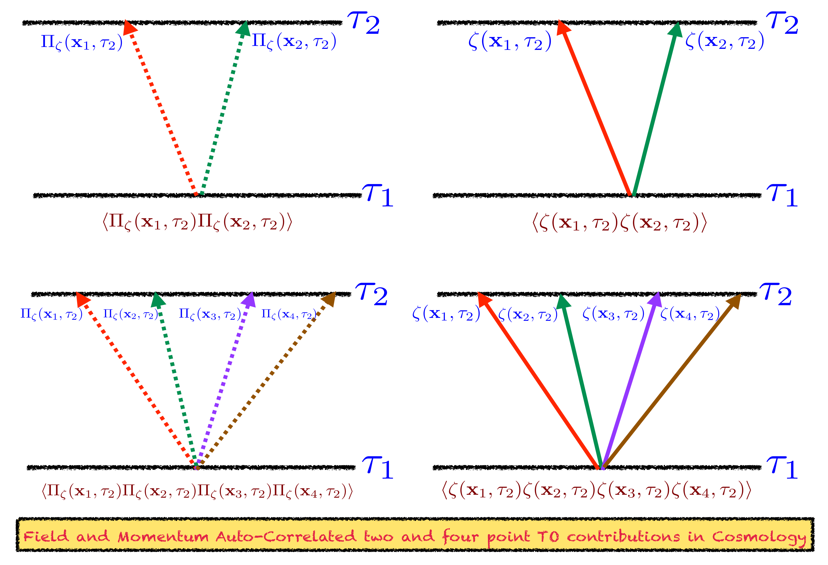
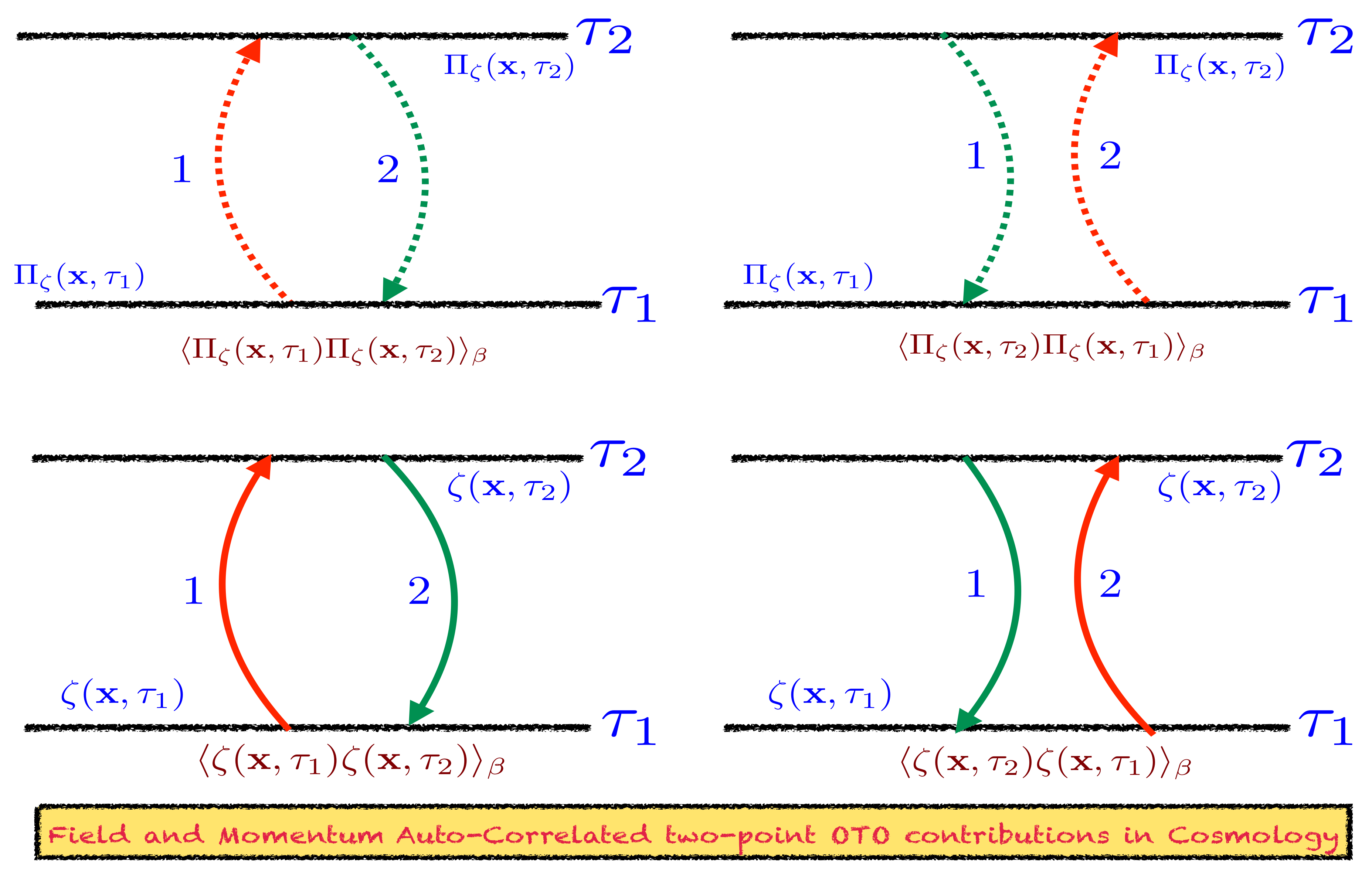
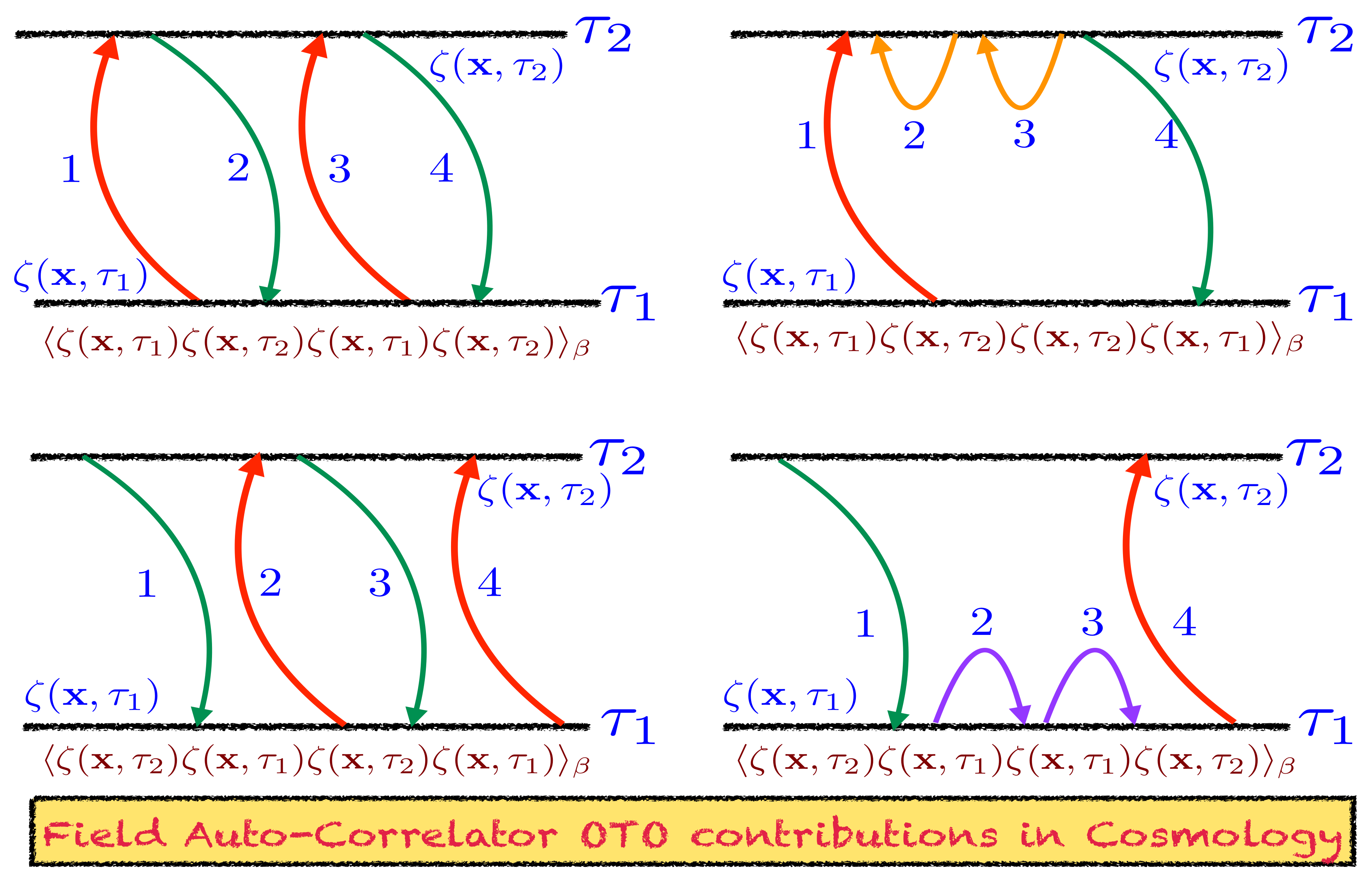
• Information II:
  In the next step, one needs to explicitly compute the expression for the commutator and square of the commutator bracket between the two perturbed field variable quantum operators and the two canonically conjugate momentum variable quantum operators defined at two different conformal time scales in the classical geometrical background of spatially flat FLRW space-time specifically in coordinate space representation. These are the crucial parts which form the building blocks of the desired OTOCs in the context of cosmological perturbation theory of the early universe. In this section of the paper, we explicitly derive the commutator and square of the commutator or these two operators in terms of two and four parts respectively where each of the components mimics the role of scattering amplitudes in Fourier space. In the present context, commutator and the square of the commutator bracket in the Fourier space involved two momenta and four momenta, respectively, and in both the cases two different conformal time scales appear which will finally fix the structure of the desired OTOCs which we want to study in the context of cosmological perturbation theory. If we look into the structure of these commutator and square of the commutator quantum mechanical operators very closely, then one can observe that these two different momenta and four different momenta are appearing in OTOCs as we are dealing with the product of two and quantum mechanical operators, respectively, in this computation. Though the OTOC computed from the square of the commutator bracket looks like $2\to 2$ scattering amplitude in the Fourier space, technically these are actually representing the unequal time, out-of-time-ordered four-point quantum correlation function in the context of cosmology. In the quantum field theory version of the trace operation, one needs to consider the same quantum initial vacuum state, which implies the initial and final state are exactly same, and identified to be “in” quantum state in the context of cosmology. This further implies that within the framework of primordial cosmology, we deal with in-in amplitude rather than using the usual “in-out” amplitude in the S-matrix formalism, which is actually a Schwinger Dyson series. Instead of calling this quantity which we want to explicitly determine in this section as “in-in” amplitude, we call these quantities as “in-in” quantum mechanical correlation functions within the framework of primordial cosmological perturbation theory.
• Information III:
  Another important issue is to fix the proper definition of the trace operation within the framework of quantum field theory written in classical spatially flat FLRW curved cosmological background. In the context of quantum field theory of curved space-time, particularly in the context of cosmology, we have to define the quantum wave function of our universe which will help us to set up the equivalent representation of the thermal trace operation in terms of the quantum mechanical path integral formulation. To construct the wave function of the universe as an initial condition, one chooses the standard definition of Euclidean false vacuum state, which is commonly known as the Bunch–Davies vacuum state and it basically represents a thermal ground state in the context of primordial cosmological perturbation theory. In the quantum field theory of curved space-time literature, sometimes this is identified to be the Hartle–Hawking or Cherenkov vacuum state. In this computation, the most generalized choice is the $\alpha ,\beta$ vacua, which is commonly known as the Motta–Allen (MA) vacua in the context of quantum field theory of De Sitter space-time, which are invariant under all the conformal group $SO(1,4)$ isometries and commonly known as the $\alpha ,\beta$-vacua which is CPT violating. Here, $\alpha ,\beta$ is a real parameter which forms a real parameter family of continuous numbers and particularly $\beta$ is appearing in the phases. This phase factor is actually the culprit for which the quantum state CPT symmetry is getting violated. Once we switch off the contribution from this phase factor by fixing $\beta =0$, the one can get back the CPT symmetry preserving quantum $\alpha$ vacua states. Sometimes the $\alpha$ vacua is characterized as the squeezed quantum vacuum state. Bunch–Davies vacuum state is a very special case of the generalized $\alpha$ vacua state which can be obtained by fixing $\alpha =0$ in the definition of the quantum vacuum state, which perfectly satisfies the Hadamard condition in the Green’s functions. Using Bogoliubov transformation, one can express the $\alpha$ vacua in terms of the Bunch Davies state.
• Information IV:
  Once we fix the definition of the quantum field theory version of the trace operation in terms of path integral formalism in the Euclidean formalism, we can then further compute the expression for the desired two sets of OTOCs on which we are interested in this paper. Another important component which will fix the definition of the OTOC is the thermal partition function for the scalar mode fluctuations obtained from the primordial cosmological perturbation where the same trick has to be applied to define the trace operation as mentioned earlier. In this context, instead of performing a complete quantum calculation, we use the semi-classical approximations for the computations. The primordial perturbations in the spatially flat classical FLRW background can be written in terms of scalar, vector and tensor modes in Fourier space using the SVT decomposition from which the quantum fluctuations are generated. For this reason, we will do a semi-classical (not purely quantum or classical) computation for the computation of OTOC in the framework of primordial cosmology.
• Information V:
  Last but not least, we have to fix the normalisation factor of all the desired new OTOCs that we have introduced in this paper. In this connection, it is important to remind ourself again that normalisation factors of these desired OTOCs are actually made up of a product of two disconnected thermal two-point functions in the dissipation time scale $t=t_d\sim \beta \sim 1/T$, where T is the equilibrium temperature of the quantum cosmological system under study in the present context. Whatever results we have obtained for the un-normalised OTOCs, we use them and divide them into the mentioned disconnected part of the correlator. This helps to treat the overall amplitude of four-point OTOCs in a dimensionless fashion. Not only that trick in normalisation but in OTOC also helps us to know about the exact time dependence in the quantum correlator of which we are interested in. More precisely, this can be done by making use of the previously mentioned equivalent operation of thermal trace operation in the presence of $\alpha$ vacua or Bunch–Davies quantum vacuum state in the context of primordial cosmological perturbation theory. We have explicitly demonstrated the detailed computation of these normalisation factors in the Appendix of this paper. Please look into the technical details in the Appendix for more details on this issue.

3.5.2. Fourier Space Representation of the Commutator Bracket: Application to Two-Point Non-Chaotic Auto-Correlated OTO Functions

Here, our job is to compute the following commutator brackets, given by the following expressions:

$$\begin{array}{ccc}& & {\mathbf{Commutator}}_{\mathbf{1}}:\left[\hat{f}(\mathbf{x},{\tau }_1),\hat{f}(\mathbf{x},{\tau }_2)\right]=\underset{\equiv {\mathsf{\Gamma }}_{\mathbf{1}}(\mathbf{x},{\mathbf{ø}}_{\mathbf{1}},{\mathbf{ø}}_{\mathbf{2}})}{\underbrace{\hat{f}(\mathbf{x},{\tau }_1)\hat{f}(\mathbf{x},{\tau }_2)}}-\underset{\equiv {\mathsf{\Gamma }}_{\mathbf{2}}(\mathbf{x},{\mathbf{ø}}_{\mathbf{1}},{\mathbf{ø}}_{\mathbf{2}})}{\underbrace{\hat{f}(\mathbf{x},{\tau }_2)\hat{f}(\mathbf{x},{\tau }_1)}},\hfill \end{array}$$

(178)

$$\begin{array}{ccc}& & {\mathbf{Commutator}}_{\mathbf{2}}:\left[\hat{\mathsf{\Pi }}(\mathbf{x},{\tau }_1),\hat{\mathsf{\Pi }}(\mathbf{x},{\tau }_2)\right]=\underset{\equiv {\mathsf{\Theta }}_{\mathbf{1}}(\mathbf{x},{\mathbf{ø}}_{\mathbf{1}},{\mathbf{ø}}_{\mathbf{2}})}{\underbrace{\hat{\mathsf{\Pi }}(\mathbf{x},{\tau }_1)\hat{\mathsf{\Pi }}(\mathbf{x},{\tau }_2)}}-\underset{\equiv {\mathsf{\Theta }}_{\mathbf{2}}(\mathbf{x},{\mathbf{ø}}_{\mathbf{1}},{\mathbf{ø}}_{\mathbf{2}})}{\underbrace{\hat{\mathsf{\Pi }}(\mathbf{x},{\tau }_2)\hat{\mathsf{\Pi }}(\mathbf{x},{\tau }_1)}}.\hfill \end{array}$$

(179)

Now we use the following preferred convention for the Fourier transformation of the perturbation field and associated momentum operator, which are given by:

$$\begin{array}{ccc}& & \hat{f}(\mathbf{x},{\tau }_1)=\int \frac{d^3\mathbf{k}}{{\left(2\pi \right)}^3}exp(i\mathbf{k}.\mathbf{x}){\hat{f}}_{\mathbf{k}}\left({\tau }_1\right),\hfill \end{array}$$

(180)

$$\begin{array}{ccc}& & \hat{\mathsf{\Pi }}(\mathbf{x},{\tau }_1)={\partial }_{{\tau }_1}\hat{f}(\mathbf{x},{\tau }_1)=\int \frac{d^3\mathbf{k}}{{\left(2\pi \right)}^3}exp(i\mathbf{k}.\mathbf{x}){\partial }_{{\tau }_1}{\hat{f}}_{\mathbf{k}}\left({\tau }_1\right)=\int \frac{d^3\mathbf{k}}{{\left(2\pi \right)}^3}exp(i\mathbf{k}.\mathbf{x}){\hat{\mathsf{\Pi }}}_{\mathbf{k}}\left({\tau }_1\right),\hfill \end{array}$$

(181)

which we will frequently follow for the rest of the computation to fix the definition of the desired OTOCs defined in this paper.

Next, we explicitly compute the expressions for these individual quantum mechanical operators in the context of primordial cosmological perturbation theory, ${\mathsf{\Gamma }}_i(\mathbf{x},{\tau }_1,{\tau }_2)$ $\forall i=1,2$ and ${\mathsf{\Theta }}_i(\mathbf{x},{\tau }_1,{\tau }_2)$ $\forall i=1,2$, which can be expressed in Fourier transformed space by the following simplified expressions:

$$\begin{array}{ccc}\hfill {\mathsf{\Gamma }}_1(\mathbf{x},{\tau }_1,{\tau }_2)& =& \hat{f}(\mathbf{x},{\tau }_1)\hat{f}(\mathbf{x},{\tau }_2)=\int \frac{d^3{\mathbf{k}}_1}{{\left(2\pi \right)}^3}\int \frac{d^3{\mathbf{k}}_1}{{\left(2\pi \right)}^3}exp(i({\mathbf{k}}_1+{\mathbf{k}}_2).\mathbf{x}){\hat{f}}_{{\mathbf{k}}_1}\left({\tau }_1\right){\hat{f}}_{{\mathbf{k}}_2}\left({\tau }_2\right)\hfill \\ & =& \int \frac{d^3{\mathbf{k}}_1}{{\left(2\pi \right)}^3}\int \frac{d^3{\mathbf{k}}_1}{{\left(2\pi \right)}^3}exp(i({\mathbf{k}}_1+{\mathbf{k}}_2).\mathbf{x}){\hat{\Delta }}_1^{\left(1\right)}({\mathbf{k}}_1,{\mathbf{k}}_2;{\tau }_1,{\tau }_2),\hfill \end{array}$$

(182)

where we have introduced a momentum- and conformal time-dependent quantum mechanical operator in the context of primordial cosmological perturbation theory, ${\hat{\Delta }}_1({\mathbf{k}}_1,{\mathbf{k}}_2;{\tau }_1,{\tau }_2)$, which is defined as:

$$\begin{array}{ccc}\hfill {\hat{\Delta }}_1^{\left(1\right)}({\mathbf{k}}_1,{\mathbf{k}}_2;{\tau }_1,{\tau }_2)& =& {\hat{f}}_{{\mathbf{k}}_1}\left({\tau }_1\right){\hat{f}}_{{\mathbf{k}}_2}\left({\tau }_2\right)={\mathcal{D}}_1^{\left(1\right)}({\mathbf{k}}_1,{\mathbf{k}}_2;{\tau }_1,{\tau }_2)a_{{\mathbf{k}}_1}{a}_{{\mathbf{k}}_2}+{\mathcal{D}}_2^{\left(1\right)}({\mathbf{k}}_1,{\mathbf{k}}_2;{\tau }_1,{\tau }_2)a_{-{\mathbf{k}}_1}^{†}{a}_{{\mathbf{k}}_2}\hfill \\ & & +{\mathcal{D}}_3^{\left(1\right)}({\mathbf{k}}_1,{\mathbf{k}}_2;{\tau }_1,{\tau }_2)a_{{\mathbf{k}}_1}{a}_{-{\mathbf{k}}_2}^{†}+{\mathcal{D}}_4^{\left(1\right)}({\mathbf{k}}_1,{\mathbf{k}}_2;{\tau }_1,{\tau }_2)a_{-{\mathbf{k}}_1}^{†}{a}_{-{\mathbf{k}}_2}^{†},\hfill \end{array}$$

(183)

where we have introduced momentum- and time-dependent two-point OTO amplitudes, ${\mathcal{D}}_i^{\left(1\right)}({\mathbf{k}}_1,{\mathbf{k}}_2;{\tau }_1,{\tau }_2)\forall i=1,2,3,4$, which are explicitly defined in Appendix B of this paper.

$$\begin{array}{ccc}\hfill {\mathsf{\Gamma }}_2(\mathbf{x},{\tau }_1,{\tau }_2)& =& \hat{\mathsf{\Pi }}(\mathbf{x},{\tau }_2)\hat{f}(\mathbf{x},{\tau }_1)=\int \frac{d^3{\mathbf{k}}_1}{{\left(2\pi \right)}^3}\int \frac{d^3{\mathbf{k}}_1}{{\left(2\pi \right)}^3}exp(i({\mathbf{k}}_1+{\mathbf{k}}_2).\mathbf{x}){\hat{\mathsf{\Pi }}}_{{\mathbf{k}}_1}\left({\tau }_2\right){\hat{f}}_{{\mathbf{k}}_2}\left({\tau }_1\right)\hfill \\ & =& \int \frac{d^3{\mathbf{k}}_1}{{\left(2\pi \right)}^3}\int \frac{d^3{\mathbf{k}}_1}{{\left(2\pi \right)}^3}exp(i({\mathbf{k}}_1+{\mathbf{k}}_2).\mathbf{x}){\hat{\Delta }}_2^{\left(1\right)}({\mathbf{k}}_1,{\mathbf{k}}_2;{\tau }_1,{\tau }_2),\hfill \end{array}$$

(184)

where we have introduced a momentum- and conformal time-dependent quantum mechanical operator in the context of primordial cosmological perturbation theory, ${\hat{\Delta }}_2^{\left(1\right)}({\mathbf{k}}_1,{\mathbf{k}}_2;{\tau }_1,{\tau }_2)$, which are explicitly defined in the Appendix of this paper.

$$\begin{array}{ccc}\hfill {\hat{\Delta }}_2^{\left(1\right)}({\mathbf{k}}_1,{\mathbf{k}}_2;{\tau }_1,{\tau }_2)& =& {\hat{f}}_{{\mathbf{k}}_1}\left({\tau }_2\right){\hat{f}}_{{\mathbf{k}}_2}\left({\tau }_1\right)={\mathcal{L}}_1^{\left(1\right)}({\mathbf{k}}_1,{\mathbf{k}}_2;{\tau }_1,{\tau }_2)a_{{\mathbf{k}}_1}{a}_{{\mathbf{k}}_2}+{\mathcal{L}}_2^{\left(1\right)}({\mathbf{k}}_1,{\mathbf{k}}_2;{\tau }_1,{\tau }_2)a_{-{\mathbf{k}}_1}^{†}{a}_{{\mathbf{k}}_2}\hfill \\ & & +{\mathcal{L}}_3^{\left(1\right)}({\mathbf{k}}_1,{\mathbf{k}}_2;{\tau }_1,{\tau }_2)a_{{\mathbf{k}}_1}{a}_{-{\mathbf{k}}_2}^{†}+{\mathcal{L}}_4^{\left(1\right)}({\mathbf{k}}_1,{\mathbf{k}}_2;{\tau }_1,{\tau }_2)a_{-{\mathbf{k}}_1}^{†}{a}_{-{\mathbf{k}}_2}^{†},\hfill \end{array}$$

(185)

where we have introduced momentum- and time-dependent two-point OTO amplitudes, ${\mathcal{L}}_i^{\left(1\right)}({\mathbf{k}}_1,{\mathbf{k}}_2;{\tau }_1,{\tau }_2)\forall i=1,2,3,4$, which are explicitly defined in the Appendix of this paper.

$$\begin{array}{ccc}\hfill {\mathsf{\Theta }}_1(\mathbf{x},{\tau }_1,{\tau }_2)& =& \hat{\mathsf{\Pi }}(\mathbf{x},{\tau }_1)\hat{\mathsf{\Pi }}(\mathbf{x},{\tau }_2)=\int \frac{d^3{\mathbf{k}}_1}{{\left(2\pi \right)}^3}\int \frac{d^3{\mathbf{k}}_1}{{\left(2\pi \right)}^3}exp(i({\mathbf{k}}_1+{\mathbf{k}}_2).\mathbf{x}){\hat{\mathsf{\Pi }}}_{{\mathbf{k}}_1}\left({\tau }_1\right){\hat{\mathsf{\Pi }}}_{{\mathbf{k}}_2}\left({\tau }_2\right)\hfill \\ & =& \int \frac{d^3{\mathbf{k}}_1}{{\left(2\pi \right)}^3}\int \frac{d^3{\mathbf{k}}_1}{{\left(2\pi \right)}^3}exp(i({\mathbf{k}}_1+{\mathbf{k}}_2).\mathbf{x}){\hat{\Delta }}_1^{\left(2\right)}({\mathbf{k}}_1,{\mathbf{k}}_2;{\tau }_1,{\tau }_2),\hfill \end{array}$$

(186)

where we have introduced a momentum- and conformal time-dependent quantum mechanical operator in the context of primordial cosmological perturbation theory, ${\hat{\Delta }}_1^{\left(2\right)}({\mathbf{k}}_1,{\mathbf{k}}_2;{\tau }_1,{\tau }_2)$, which are explicitly defined in the Appendix of this paper as:

$$\begin{array}{ccc}\hfill {\hat{\Delta }}_1^{\left(2\right)}({\mathbf{k}}_1,{\mathbf{k}}_2;{\tau }_1,{\tau }_2)& =& {\hat{\mathsf{\Pi }}}_{{\mathbf{k}}_1}\left({\tau }_1\right){\hat{\mathsf{\Pi }}}_{{\mathbf{k}}_2}\left({\tau }_2\right)={\mathcal{D}}_1^{\left(2\right)}({\mathbf{k}}_1,{\mathbf{k}}_2;{\tau }_1,{\tau }_2)a_{{\mathbf{k}}_1}{a}_{{\mathbf{k}}_2}+{\mathcal{D}}_2^{\left(2\right)}({\mathbf{k}}_1,{\mathbf{k}}_2;{\tau }_1,{\tau }_2)a_{-{\mathbf{k}}_1}^{†}{a}_{{\mathbf{k}}_2}\hfill \\ & & +{\mathcal{D}}_3^{\left(2\right)}({\mathbf{k}}_1,{\mathbf{k}}_2;{\tau }_1,{\tau }_2)a_{{\mathbf{k}}_1}{a}_{-{\mathbf{k}}_2}^{†}+{\mathcal{D}}_4^{\left(2\right)}({\mathbf{k}}_1,{\mathbf{k}}_2;{\tau }_1,{\tau }_2)a_{-{\mathbf{k}}_1}^{†}{a}_{-{\mathbf{k}}_2}^{†},\hfill \end{array}$$

(187)

where we have introduced momentum- and time-dependent two-point OTO amplitudes, ${\mathcal{D}}_i^{\left(2\right)}({\mathbf{k}}_1,{\mathbf{k}}_2;{\tau }_1,{\tau }_2)\forall i=1,2,3,4$, which are explicitly defined in the Appendix of this paper.

$$\begin{array}{ccc}\hfill {\mathsf{\Theta }}_2(\mathbf{x},{\tau }_1,{\tau }_2)& =& \hat{\mathsf{\Pi }}(\mathbf{x},{\tau }_2)\hat{\mathsf{\Pi }}(\mathbf{x},{\tau }_1)=\int \frac{d^3{\mathbf{k}}_1}{{\left(2\pi \right)}^3}\int \frac{d^3{\mathbf{k}}_1}{{\left(2\pi \right)}^3}exp(i({\mathbf{k}}_1+{\mathbf{k}}_2).\mathbf{x}){\hat{\mathsf{\Pi }}}_{{\mathbf{k}}_1}\left({\tau }_2\right){\hat{\mathsf{\Pi }}}_{{\mathbf{k}}_2}\left({\tau }_1\right)\hfill \\ & =& \int \frac{d^3{\mathbf{k}}_1}{{\left(2\pi \right)}^3}\int \frac{d^3{\mathbf{k}}_1}{{\left(2\pi \right)}^3}exp(i({\mathbf{k}}_1+{\mathbf{k}}_2).\mathbf{x}){\hat{\Delta }}_2^{\left(2\right)}({\mathbf{k}}_1,{\mathbf{k}}_2;{\tau }_1,{\tau }_2),\hfill \end{array}$$

(188)

where we have introduced a momentum- and conformal time-dependent quantum mechanical operator ${\hat{\Delta }}_2({\mathbf{k}}_1,{\mathbf{k}}_2;{\tau }_1,{\tau }_2)$, which is defined as:

$$\begin{array}{ccc}\hfill {\hat{\Delta }}_2^{\left(2\right)}({\mathbf{k}}_1,{\mathbf{k}}_2;{\tau }_1,{\tau }_2)& =& {\hat{\mathsf{\Pi }}}_{{\mathbf{k}}_1}\left({\tau }_2\right){\hat{\mathsf{\Pi }}}_{{\mathbf{k}}_2}\left({\tau }_1\right)\hfill \\ & =& {\mathcal{L}}_1^{\left(2\right)}({\mathbf{k}}_1,{\mathbf{k}}_2;{\tau }_1,{\tau }_2)a_{{\mathbf{k}}_1}{a}_{{\mathbf{k}}_2}+{\mathcal{L}}_2^{\left(2\right)}({\mathbf{k}}_1,{\mathbf{k}}_2;{\tau }_1,{\tau }_2)a_{-{\mathbf{k}}_1}^{†}{a}_{{\mathbf{k}}_2}\hfill \\ & & +{\mathcal{L}}_3^{\left(2\right)}({\mathbf{k}}_1,{\mathbf{k}}_2;{\tau }_1,{\tau }_2)a_{{\mathbf{k}}_1}{a}_{-{\mathbf{k}}_2}^{†}+{\mathcal{L}}_4^{\left(2\right)}({\mathbf{k}}_1,{\mathbf{k}}_2;{\tau }_1,{\tau }_2)a_{-{\mathbf{k}}_1}^{†}{a}_{-{\mathbf{k}}_2}^{†},\hfill \end{array}$$

(189)

where we have introduced momentum- and time-dependent two-point OTO amplitudes, ${\mathcal{L}}_i^{\left(2\right)}({\mathbf{k}}_1,{\mathbf{k}}_2;{\tau }_1,{\tau }_2)\forall i=1,2,3,4$, which are explicitly defined in Appendix B of this paper.

This further implies that one can explicitly write down the previously mentioned two commutator brackets along with the thermal Boltzmann factor in terms of the following simplified expression, which is given by:

$$\begin{array}{ccc}& & e^{-\beta \hat{H}\left({\tau }_1\right)}\left[\hat{f}(\mathbf{x},{\tau }_1),\hat{f}(\mathbf{x},{\tau }_2)\right]\hfill \\ & & =e^{-\beta \hat{H}\left({\tau }_1\right)}\left[{\mathsf{\Gamma }}_1(\mathbf{x},{\tau }_1,{\tau }_2)-{\mathsf{\Gamma }}_2(\mathbf{x},{\tau }_1,{\tau }_2)\right]\hfill \\ & & =e^{-\beta \hat{H}\left({\tau }_1\right)}\left\{\int \frac{d^3{k}_1}{{\left(2\pi \right)}^3}\int \frac{d^3{k}_2}{{\left(2\pi \right)}^3}exp\left[i\left({\mathbf{k}}_1+{\mathbf{k}}_2\right).\mathbf{x}\right]\left[{\hat{\Delta }}_1^{\left(1\right)}({\mathbf{k}}_1,{\mathbf{k}}_2;{\tau }_1,{\tau }_2)-{\hat{\Delta }}_2^{\left(1\right)}({\mathbf{k}}_1,{\mathbf{k}}_2;{\tau }_1,{\tau }_2)\right]\right\}\hfill \\ & & =\int \frac{d^3{k}_1}{{\left(2\pi \right)}^3}\int \frac{d^3{k}_2}{{\left(2\pi \right)}^3}exp\left[i\left({\mathbf{k}}_1+{\mathbf{k}}_2\right).\mathbf{x}\right]\left[{\hat{\nabla }}_1^{\left(1\right)}({\mathbf{k}}_1,{\mathbf{k}}_2;{\tau }_1,{\tau }_2;\beta )-{\hat{\nabla }}_2^{\left(1\right)}({\mathbf{k}}_1,{\mathbf{k}}_2;{\tau }_1,{\tau }_2;\beta )\right],\hfill \end{array}$$

(190)

$$\begin{array}{ccc}& & e^{-\beta \hat{H}\left({\tau }_1\right)}\left[\hat{\mathsf{\Pi }}(\mathbf{x},{\tau }_1),\hat{\mathsf{\Pi }}(\mathbf{x},{\tau }_2)\right]\hfill \\ & & =e^{-\beta \hat{H}\left({\tau }_1\right)}\left[{\mathsf{\Theta }}_1(\mathbf{x},{\tau }_1,{\tau }_2)-{\mathsf{\Theta }}_2(\mathbf{x},{\tau }_1,{\tau }_2)\right]\hfill \\ & & =e^{-\beta \hat{H}\left({\tau }_1\right)}\left\{\int \frac{d^3{k}_1}{{\left(2\pi \right)}^3}\int \frac{d^3{k}_2}{{\left(2\pi \right)}^3}exp\left[i\left({\mathbf{k}}_1+{\mathbf{k}}_2\right).\mathbf{x}\right]\left[{\hat{\Delta }}_1^{\left(2\right)}({\mathbf{k}}_1,{\mathbf{k}}_2;{\tau }_1,{\tau }_2)-{\hat{\Delta }}_2^{\left(2\right)}({\mathbf{k}}_1,{\mathbf{k}}_2;{\tau }_1,{\tau }_2)\right]\right\}\hfill \\ & & =\int \frac{d^3{k}_1}{{\left(2\pi \right)}^3}\int \frac{d^3{k}_2}{{\left(2\pi \right)}^3}exp\left[i\left({\mathbf{k}}_1+{\mathbf{k}}_2\right).\mathbf{x}\right]\left[{\hat{\nabla }}_1^{\left(2\right)}({\mathbf{k}}_1,{\mathbf{k}}_2;{\tau }_1,{\tau }_2;\beta )-{\hat{\nabla }}_2^{\left(2\right)}({\mathbf{k}}_1,{\mathbf{k}}_2;{\tau }_1,{\tau }_2;\beta )\right],\hfill \end{array}$$

(191)

where we define the new sets of quantum mechanical operators in the context of primordial cosmological perturbation theory, ${\hat{\nabla }}_i^{\left(m\right)}({\mathbf{k}}_1,{\mathbf{k}}_2;{\tau }_1,{\tau }_2;\beta ):\forall i=1,2,\forall m=1,2$ as given by the following expression:

$$\begin{array}{ccc}& & {\hat{\nabla }}_i^{\left(m\right)}({\mathbf{k}}_1,{\mathbf{k}}_2;{\tau }_1,{\tau }_2;\beta )=e^{-\beta \hat{H}\left({\tau }_1\right)}{\hat{\Delta }}_i^{\left(m\right)}({\mathbf{k}}_1,{\mathbf{k}}_2;{\tau }_1,{\tau }_2)\forall i=1,2\forall m=1,2\hfill \end{array}$$

(192)

Here the thermal Boltzmann factor can be expressed in terms of creation and annihilation operator by the following simplified expression, as given by:

$$\begin{array}{ccc}& & e^{-\beta H\left({\tau }_1\right)}=exp\left(-\beta \int d^3\mathbf{k}\left({\widehat{\mathcal{N}}}_{\mathbf{k}}+\frac{1}{2}{\delta }^3\left(0\right)\right)E_{\mathbf{k}}\left({\tau }_1\right)\right),\hfill \end{array}$$

(193)

where we define the conformal time-dependent energy spectrum as a function of Fourier modes relevant for cosmology, $E_{\mathbf{k}}\left({\tau }_1\right)$, by the following expression:

$$\begin{array}{c}\hfill E_{\mathbf{k}}\left({\tau }_1\right):=\left[|{\mathsf{\Pi }}_{\mathbf{k}}\left({\tau }_1\right){|}^2+{\omega }_{\mathbf{k}}^2\left({\tau }_1\right){\left|f_{\mathbf{k}}\left(\tau \right)\right|}^2\right],\end{array}$$

(194)

where the explicit expression for the conformal time-dependent expression for the frequency factor at the time scale $\tau ={\tau }_1$, i.e., ${\omega }_{\mathbf{k}}\left({\tau }_1\right)$ for the cosmologically relevant Fourier modes participating in the primordial cosmological perturbation theory, is mentioned in the earlier half of this paper. For general readers, it is further important to note that these mode frequencies for all momentum scales play a significant role for the quantification of the randomness in terms of the quantum OTOCs studied in this paper.

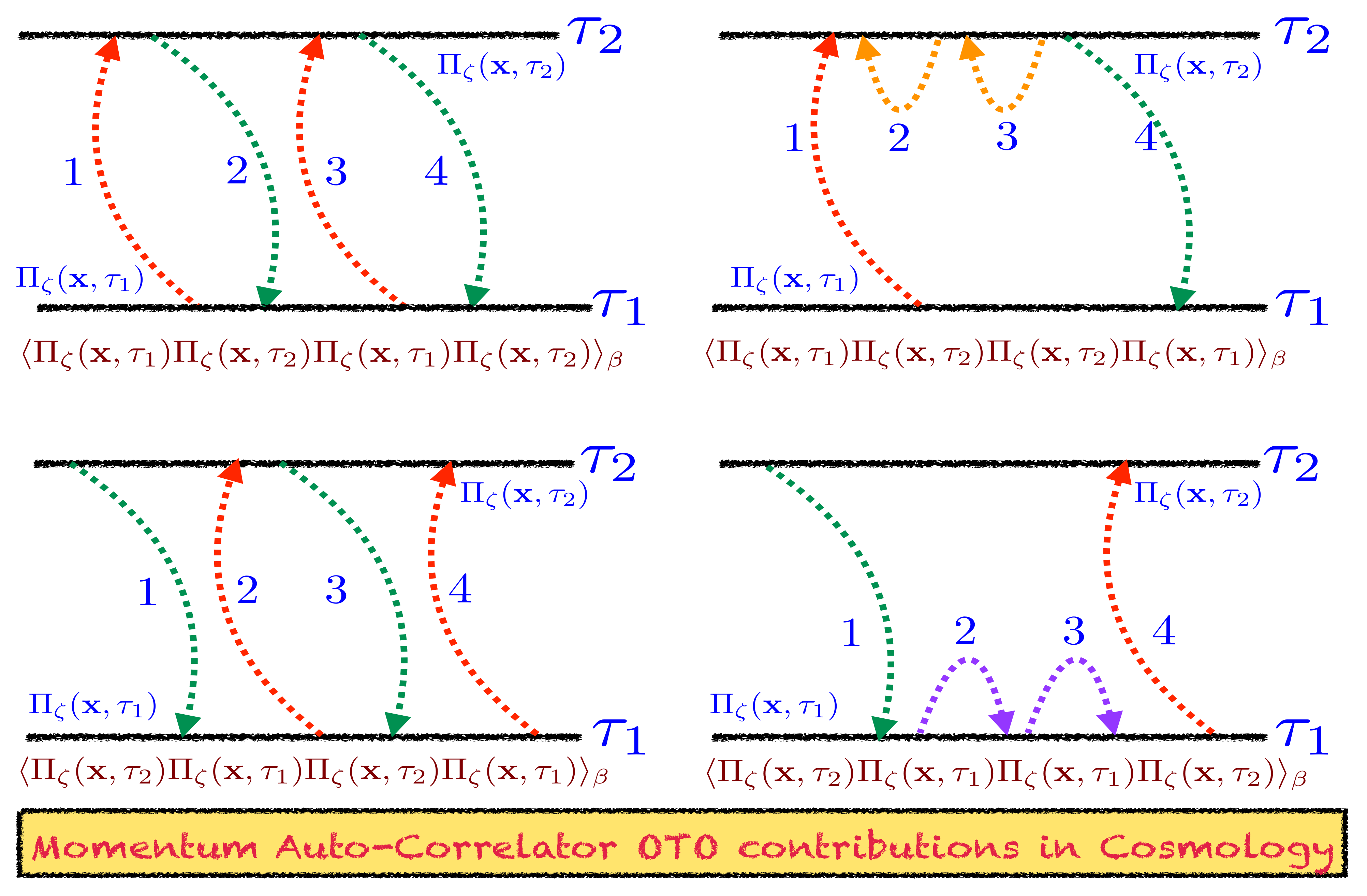
3.5.3. Fourier Space Representation of Square of the Commutator Bracket: Application to Four-Point Non-Chaotic Auto-Correlated OTO Functions

Now we explicitly compute the following combinations of the square of the commutator bracket out of only the cosmologically perturbed field operators and only with the help of the canonically conjugate momentum operators related to these cosmologically perturbed field, which are actually given by the following simplified expression:

$$\begin{array}{ccc}& & {\left[\hat{f}(\mathbf{x},{\tau }_1),\hat{f}(\mathbf{x},{\tau }_2)\right]}^2=\underset{\equiv {\mathcal{K}}_1^{\left(1\right)}(\mathbf{x},{\tau }_1,{\tau }_2)}{\underbrace{\hat{f}(\mathbf{x},{\tau }_1)\hat{f}(\mathbf{x},{\tau }_2)\hat{f}(\mathbf{x},{\tau }_1)\hat{f}(\mathbf{x},{\tau }_2)}}-\underset{\equiv {\mathcal{K}}_2^{\left(1\right)}(\mathbf{x},{\tau }_1,{\tau }_2)}{\underbrace{\hat{f}(\mathbf{x},{\tau }_2)\hat{f}(\mathbf{x},{\tau }_1)\hat{f}(\mathbf{x},{\tau }_1)\hat{f}(\mathbf{x},{\tau }_2)}}\hfill \\ & & -\underset{\equiv {\mathcal{K}}_3^{\left(1\right)}(\mathbf{x},{\tau }_1,{\tau }_2)}{\underbrace{\hat{f}(\mathbf{x},{\tau }_1)\hat{f}(\mathbf{x},{\tau }_2)\hat{f}(\mathbf{x},{\tau }_2)\hat{f}(\mathbf{x},{\tau }_1)}}+\underset{\equiv {\mathcal{K}}_4^{\left(1\right)}(\mathbf{x},{\tau }_1,{\tau }_2)}{\underbrace{\hat{f}(\mathbf{x},{\tau }_2)\hat{f}(\mathbf{x},{\tau }_1)\hat{f}(\mathbf{x},{\tau }_2)\hat{f}(\mathbf{x},{\tau }_1)}},\hfill \end{array}$$

(195)

$$\begin{array}{ccc}& & {\left[\hat{\mathsf{\Pi }}(\mathbf{x},{\tau }_1),\hat{\mathsf{\Pi }}(\mathbf{x},{\tau }_2)\right]}^2=\underset{\equiv {\mathcal{K}}_1^{\left(2\right)}(\mathbf{x},{\tau }_1,{\tau }_2)}{\underbrace{\hat{\mathsf{\Pi }}(\mathbf{x},{\tau }_1)\hat{\mathsf{\Pi }}(\mathbf{x},{\tau }_2)\hat{\mathsf{\Pi }}(\mathbf{x},{\tau }_1)\hat{\mathsf{\Pi }}(\mathbf{x},{\tau }_2)}}-\underset{\equiv {\mathcal{K}}_2^{\left(2\right)}(\mathbf{x},{\tau }_1,{\tau }_2)}{\underbrace{\hat{\mathsf{\Pi }}(\mathbf{x},{\tau }_2)\hat{\mathsf{\Pi }}(\mathbf{x},{\tau }_1)\hat{\mathsf{\Pi }}(\mathbf{x},{\tau }_1)\hat{\mathsf{\Pi }}(\mathbf{x},{\tau }_2)}}\hfill \\ & & -\underset{\equiv {\mathcal{K}}_3^{\left(2\right)}(\mathbf{x},{\tau }_1,{\tau }_2)}{\underbrace{\hat{\mathsf{\Pi }}(\mathbf{x},{\tau }_1)\hat{\mathsf{\Pi }}(\mathbf{x},{\tau }_2)\hat{\mathsf{\Pi }}(\mathbf{x},{\tau }_2)\hat{\mathsf{\Pi }}(\mathbf{x},{\tau }_1)}}+\underset{\equiv {\mathcal{K}}_4^{\left(2\right)}(\mathbf{x},{\tau }_1,{\tau }_2)}{\underbrace{\hat{\mathsf{\Pi }}(\mathbf{x},{\tau }_2)\hat{\mathsf{\Pi }}(\mathbf{x},{\tau }_1)\hat{\mathsf{\Pi }}(\mathbf{x},{\tau }_2)\hat{\mathsf{\Pi }}(\mathbf{x},{\tau }_1)}}\hfill \end{array}$$

(196)

Now we mention the explicit mathematical structure of these individual operators, ${\mathcal{K}}_i^{\left(M\right)}(\mathbf{x},{\tau }_1,{\tau }_2)\forall i=1,2,3,4,\forall M=1,2,3,4$, which are expressed in Fourier transformed space as:

$$\begin{array}{ccc}& & {\mathcal{K}}_1^{\left(1\right)}(\mathbf{x},{\tau }_1,{\tau }_2)=\hat{f}(\mathbf{x},{\tau }_1)\hat{f}(\mathbf{x},{\tau }_2)\hat{f}(\mathbf{x},{\tau }_1)\hat{f}(\mathbf{x},{\tau }_2)\hfill \\ & & =\int \frac{d^3{k}_1}{{\left(2\pi \right)}^3}\int \frac{d^3{k}_2}{{\left(2\pi \right)}^3}\int \frac{d^3{k}_3}{{\left(2\pi \right)}^3}\int \frac{d^3{k}_4}{{\left(2\pi \right)}^3}exp\left[i\left({\mathbf{k}}_1+{\mathbf{k}}_2+{\mathbf{k}}_3+{\mathbf{k}}_4\right).\mathbf{x}\right]{\widehat{\mathcal{T}}}_1^{\left(1\right)}({\mathbf{k}}_1,{\mathbf{k}}_2,{\mathbf{k}}_3,{\mathbf{k}}_4;{\tau }_1,{\tau }_2),\hfill \end{array}$$

(197)

$$\begin{array}{ccc}& & {\mathcal{K}}_1^{\left(2\right)}(\mathbf{x},{\tau }_1,{\tau }_2)=\hat{\mathsf{\Pi }}(\mathbf{x},{\tau }_1)\hat{\mathsf{\Pi }}(\mathbf{x},{\tau }_2)\hat{\mathsf{\Pi }}(\mathbf{x},{\tau }_1)\hat{\mathsf{\Pi }}(\mathbf{x},{\tau }_2)\hfill \\ & & =\int \frac{d^3{k}_1}{{\left(2\pi \right)}^3}\int \frac{d^3{k}_2}{{\left(2\pi \right)}^3}\int \frac{d^3{k}_3}{{\left(2\pi \right)}^3}\int \frac{d^3{k}_4}{{\left(2\pi \right)}^3}exp\left[i\left({\mathbf{k}}_1+{\mathbf{k}}_2+{\mathbf{k}}_3+{\mathbf{k}}_4\right).\mathbf{x}\right]{\widehat{\mathcal{T}}}_1^{\left(2\right)}({\mathbf{k}}_1,{\mathbf{k}}_2,{\mathbf{k}}_3,{\mathbf{k}}_4;{\tau }_1,{\tau }_2),\hfill \end{array}$$

(198)

$$\begin{array}{ccc}& & {\mathcal{K}}_2^{\left(1\right)}(\mathbf{x},{\tau }_1,{\tau }_2)=\hat{f}(\mathbf{x},{\tau }_2)\hat{f}(\mathbf{x},{\tau }_1)\hat{f}(\mathbf{x},{\tau }_1)\hat{f}(\mathbf{x},{\tau }_2)\hfill \\ & & =\int \frac{d^3{k}_1}{{\left(2\pi \right)}^3}\int \frac{d^3{k}_2}{{\left(2\pi \right)}^3}\int \frac{d^3{k}_3}{{\left(2\pi \right)}^3}\int \frac{d^3{k}_4}{{\left(2\pi \right)}^3}exp\left[i\left({\mathbf{k}}_1+{\mathbf{k}}_2+{\mathbf{k}}_3+{\mathbf{k}}_4\right).\mathbf{x}\right]{\widehat{\mathcal{T}}}_2^{\left(1\right)}({\mathbf{k}}_1,{\mathbf{k}}_2,{\mathbf{k}}_3,{\mathbf{k}}_4;{\tau }_1,{\tau }_2),\hfill \end{array}$$

(199)

$$\begin{array}{ccc}& & {\mathcal{K}}_2^{\left(2\right)}(\mathbf{x},{\tau }_1,{\tau }_2)=\hat{\mathsf{\Pi }}(\mathbf{x},{\tau }_2)\hat{\mathsf{\Pi }}(\mathbf{x},{\tau }_1)\hat{\mathsf{\Pi }}(\mathbf{x},{\tau }_1)\hat{\mathsf{\Pi }}(\mathbf{x},{\tau }_2)\hfill \\ & & =\int \frac{d^3{k}_1}{{\left(2\pi \right)}^3}\int \frac{d^3{k}_2}{{\left(2\pi \right)}^3}\int \frac{d^3{k}_3}{{\left(2\pi \right)}^3}\int \frac{d^3{k}_4}{{\left(2\pi \right)}^3}exp\left[i\left({\mathbf{k}}_1+{\mathbf{k}}_2+{\mathbf{k}}_3+{\mathbf{k}}_4\right).\mathbf{x}\right]{\widehat{\mathcal{T}}}_2^{\left(2\right)}({\mathbf{k}}_1,{\mathbf{k}}_2,{\mathbf{k}}_3,{\mathbf{k}}_4;{\tau }_1,{\tau }_2),\hfill \end{array}$$

(200)

$$\begin{array}{ccc}& & {\mathcal{K}}_3^{\left(1\right)}(\mathbf{x},{\tau }_1,{\tau }_2)=\hat{f}(\mathbf{x},{\tau }_1)\hat{f}(\mathbf{x},{\tau }_2)\hat{f}(\mathbf{x},{\tau }_2)\hat{f}(\mathbf{x},{\tau }_1)\hfill \\ & & =\int \frac{d^3{k}_1}{{\left(2\pi \right)}^3}\int \frac{d^3{k}_2}{{\left(2\pi \right)}^3}\int \frac{d^3{k}_3}{{\left(2\pi \right)}^3}\int \frac{d^3{k}_4}{{\left(2\pi \right)}^3}exp\left[i\left({\mathbf{k}}_1+{\mathbf{k}}_2+{\mathbf{k}}_3+{\mathbf{k}}_4\right).\mathbf{x}\right]{\widehat{\mathcal{T}}}_3^{\left(1\right)}({\mathbf{k}}_1,{\mathbf{k}}_2,{\mathbf{k}}_3,{\mathbf{k}}_4;{\tau }_1,{\tau }_2),\hfill \end{array}$$

(201)

$$\begin{array}{ccc}& & {\mathcal{K}}_3^{\left(2\right)}(\mathbf{x},{\tau }_1,{\tau }_2)=\hat{\mathsf{\Pi }}(\mathbf{x},{\tau }_1)\hat{\mathsf{\Pi }}(\mathbf{x},{\tau }_2)\hat{\mathsf{\Pi }}(\mathbf{x},{\tau }_2)\hat{\mathsf{\Pi }}(\mathbf{x},{\tau }_1)\hfill \\ & & =\int \frac{d^3{k}_1}{{\left(2\pi \right)}^3}\int \frac{d^3{k}_2}{{\left(2\pi \right)}^3}\int \frac{d^3{k}_3}{{\left(2\pi \right)}^3}\int \frac{d^3{k}_4}{{\left(2\pi \right)}^3}exp\left[i\left({\mathbf{k}}_1+{\mathbf{k}}_2+{\mathbf{k}}_3+{\mathbf{k}}_4\right).\mathbf{x}\right]{\widehat{\mathcal{T}}}_3^{\left(2\right)}({\mathbf{k}}_1,{\mathbf{k}}_2,{\mathbf{k}}_3,{\mathbf{k}}_4;{\tau }_1,{\tau }_2),\hfill \end{array}$$

(202)

$$\begin{array}{ccc}& & {\mathcal{K}}_4^{\left(1\right)}(\mathbf{x},{\tau }_1,{\tau }_2)=\hat{f}(\mathbf{x},{\tau }_2)\hat{f}(\mathbf{x},{\tau }_1)\hat{f}(\mathbf{x},{\tau }_2)\hat{f}(\mathbf{x},{\tau }_1)\hfill \\ & & =\int \frac{d^3{k}_1}{{\left(2\pi \right)}^3}\int \frac{d^3{k}_2}{{\left(2\pi \right)}^3}\int \frac{d^3{k}_3}{{\left(2\pi \right)}^3}\int \frac{d^3{k}_4}{{\left(2\pi \right)}^3}exp\left[i\left({\mathbf{k}}_1+{\mathbf{k}}_2+{\mathbf{k}}_3+{\mathbf{k}}_4\right).\mathbf{x}\right]{\widehat{\mathcal{T}}}_4^{\left(1\right)}({\mathbf{k}}_1,{\mathbf{k}}_2,{\mathbf{k}}_3,{\mathbf{k}}_4;{\tau }_1,{\tau }_2),\hfill \end{array}$$

(203)

$$\begin{array}{ccc}& & {\mathcal{K}}_4^{\left(2\right)}(\mathbf{x},{\tau }_1,{\tau }_2)=\hat{\mathsf{\Pi }}(\mathbf{x},{\tau }_2)\widehat{\mathsf{\Pi }}(\mathbf{x},{\tau }_1)\hat{\mathsf{\Pi }}(\mathbf{x},{\tau }_2)\hat{\mathsf{\Pi }}(\mathbf{x},{\tau }_1)\hfill \\ & & =\int \frac{d^3{k}_1}{{\left(2\pi \right)}^3}\int \frac{d^3{k}_2}{{\left(2\pi \right)}^3}\int \frac{d^3{k}_3}{{\left(2\pi \right)}^3}\int \frac{d^3{k}_4}{{\left(2\pi \right)}^3}exp\left[i\left({\mathbf{k}}_1+{\mathbf{k}}_2+{\mathbf{k}}_3+{\mathbf{k}}_4\right).\mathbf{x}\right]{\widehat{\mathcal{T}}}_4^{\left(2\right)}({\mathbf{k}}_1,{\mathbf{k}}_2,{\mathbf{k}}_3,{\mathbf{k}}_4;{\tau }_1,{\tau }_2),\hfill \end{array}$$

(204)

where the functions ${\widehat{\mathcal{T}}}_p^{\left(1\right)}({\mathbf{k}}_1,{\mathbf{k}}_2,{\mathbf{k}}_3,{\mathbf{k}}_4;{\tau }_1,{\tau }_2)\forall p=1,2,3,4$ and ${\widehat{\mathcal{T}}}_p^{\left(2\right)}({\mathbf{k}}_1,{\mathbf{k}}_2,{\mathbf{k}}_3,{\mathbf{k}}_4;{\tau }_1,{\tau }_2)$$\forall p=1,2,3,4$ are explicitly defined in Appendix C.

This implies that one can write down the previously mentioned square of the commutator bracket along with the thermal Boltzmann factor as:

$$\begin{array}{ccc}& & e^{-\beta \hat{H}\left({\tau }_1\right)}{\left[\hat{f}(\mathbf{x},{\tau }_1),\hat{\mathsf{\Pi }}(\mathbf{x},{\tau }_2)\right]}^2\hfill \\ & & =\int \frac{d^3{k}_1}{{\left(2\pi \right)}^3}\int \frac{d^3{k}_2}{{\left(2\pi \right)}^3}\int \frac{d^3{k}_3}{{\left(2\pi \right)}^3}\int \frac{d^3{k}_4}{{\left(2\pi \right)}^3}exp\left[i\left({\mathbf{k}}_1+{\mathbf{k}}_2+{\mathbf{k}}_3+{\mathbf{k}}_4\right).\mathbf{x}\right]\hfill \\ & & \left[{\widehat{\mathcal{V}}}_1^{\left(1\right)}({\mathbf{k}}_1,{\mathbf{k}}_2,{\mathbf{k}}_3,{\mathbf{k}}_4;{\tau }_1,{\tau }_2;\beta )-{\widehat{\mathcal{V}}}_2^{\left(1\right)}({\mathbf{k}}_1,{\mathbf{k}}_2,{\mathbf{k}}_3,{\mathbf{k}}_4;{\tau }_1,{\tau }_2;\beta )\right.\hfill \\ & & \left.+{\widehat{\mathcal{V}}}_3^{\left(1\right)}({\mathbf{k}}_1,{\mathbf{k}}_2,{\mathbf{k}}_3,{\mathbf{k}}_4;{\tau }_1,{\tau }_2;\beta )-{\widehat{\mathcal{V}}}_4^{\left(1\right)}({\mathbf{k}}_1,{\mathbf{k}}_2,{\mathbf{k}}_3,{\mathbf{k}}_4;{\tau }_1,{\tau }_2;\beta )\right],\hfill \end{array}$$

(205)

$$\begin{array}{ccc}& & e^{-\beta \hat{H}\left({\tau }_1\right)}{\left[\hat{\mathsf{\Pi }}(\mathbf{x},{\tau }_1),\hat{\mathsf{\Pi }}(\mathbf{x},{\tau }_2)\right]}^2\hfill \\ & & =\int \frac{d^3{k}_1}{{\left(2\pi \right)}^3}\int \frac{d^3{k}_2}{{\left(2\pi \right)}^3}\int \frac{d^3{k}_3}{{\left(2\pi \right)}^3}\int \frac{d^3{k}_4}{{\left(2\pi \right)}^3}exp\left[i\left({\mathbf{k}}_1+{\mathbf{k}}_2+{\mathbf{k}}_3+{\mathbf{k}}_4\right).\mathbf{x}\right]\hfill \\ & & \left[{\widehat{\mathcal{V}}}_1^{\left(2\right)}({\mathbf{k}}_1,{\mathbf{k}}_2,{\mathbf{k}}_3,{\mathbf{k}}_4;{\tau }_1,{\tau }_2;\beta )-{\widehat{\mathcal{V}}}_2^{\left(2\right)}({\mathbf{k}}_1,{\mathbf{k}}_2,{\mathbf{k}}_3,{\mathbf{k}}_4;{\tau }_1,{\tau }_2;\beta )\right.\hfill \\ & & \left.+{\widehat{\mathcal{V}}}_3^{\left(2\right)}({\mathbf{k}}_1,{\mathbf{k}}_2,{\mathbf{k}}_3,{\mathbf{k}}_4;{\tau }_1,{\tau }_2;\beta )-{\widehat{\mathcal{V}}}_4^{\left(2\right)}({\mathbf{k}}_1,{\mathbf{k}}_2,{\mathbf{k}}_3,{\mathbf{k}}_4;{\tau }_1,{\tau }_2;\beta )\right],\hfill \end{array}$$

(206)

where we define the new sets of quantum operators in the context of primordial cosmological perturbation theory setup, ${\widehat{\mathcal{V}}}_i^{\left(M\right)}({\mathbf{k}}_1,{\mathbf{k}}_2,{\mathbf{k}}_3,{\mathbf{k}}_4;{\tau }_1,{\tau }_2;\beta )\forall i=1,2,3,4,\forall M=1,2$, as given by the following simplified expression:

$$\begin{array}{ccc}& & {\widehat{\mathcal{V}}}_i^{\left(M\right)}({\mathbf{k}}_1,{\mathbf{k}}_2,{\mathbf{k}}_3,{\mathbf{k}}_4;{\tau }_1,{\tau }_2;\beta )=e^{-\beta \hat{H}\left({\tau }_1\right)}{\widehat{\mathcal{T}}}_i({\mathbf{k}}_1,{\mathbf{k}}_2,{\mathbf{k}}_3,{\mathbf{k}}_4;{\tau }_1,{\tau }_2)\forall i=1,2,3,4,M=1,2\hfill \end{array}$$

(207)

where the thermal Boltzmann factor with energy dispersion is computed earlier.

3.6. Thermal Partition Function in Primordial Cosmology: Quantum Version

3.6.1. Initial Quantum State in Primordial Cosmology

In general, one can consider an arbitrary initial quantum mechanical vacuum state which is characterized by the two arbitrary constants ${\mathcal{C}}_1$ and ${\mathcal{C}}_2$, which are appearing in the solution of the Mukhanov–Sasaki equation, which represents the classical solution of the background perturbation in the spatially flat FLRW cosmological background. In addition, these arbitrary constants play a very significant role in fixing the definition of the quantum wave function of the universe which is dependent on specified information of the initial quantum vacuum state for cosmology. Once this definition is fixed, using this quantum vacuum state one can further study the correlation function from the quantum fluctuation in the scalar modes which are contributing in terms of the co-moving scalar curvature perturbation or in terms of the redefined perturbed field variable. Now, if we say that ${\mathcal{C}}_{\mathbf{k},\mathbf{12}}$ is the annihilation operator corresponding to the quantum state as mentioned earlier, then it satisfies the following criteria in the context of quantum field theory written for the primordial cosmological perturbation:

$$\begin{array}{c}\hfill {\mathcal{C}}_{\mathbf{k},\mathbf{12}}|{\mathcal{C}}_1,{\mathcal{C}}_2{\rangle =0\forall \mathbf{k},\mathrm{with}|\Psi \rangle }_{\mathbf{QVac}}:\equiv |{\mathcal{C}}_1,{\mathcal{C}}_2\rangle \end{array}$$

(208)

In a most generalized prescription, this arbitrary quantum vacuum state can be written in terms of the ground state, which in cosmology is commonly known as the Bunch–Davies Euclidean vacuum state by the following expression:

$$\begin{array}{ccc}\hfill {|\Psi \rangle }_{\mathbf{QVac}}:\equiv |{\mathcal{C}}_1,{\mathcal{C}}_2\rangle & =& \prod _{\mathbf{k}}\frac{1}{\sqrt{|{\mathcal{C}}_1|}}exp\left(-\frac{i{\mathcal{C}}_2^{*}}{2{\mathcal{C}}_1^{*}}{a}_{\mathbf{k}}^{†}{a}_{\mathbf{k}}^{†}\right){|\Psi \rangle }_{\mathbf{BD}}=\frac{1}{\sqrt{|{\mathcal{C}}_1|}}exp\left(-\frac{i{\mathcal{C}}_2^{*}}{2{\mathcal{C}}_1^{*}}\sum _{\mathbf{k}}{a}_{\mathbf{k}}^{†}{a}_{\mathbf{k}}^{†}\right){|\Psi \rangle }_{\mathbf{BD}}\hfill \end{array}$$

(209)

Now we will use the following replacement rule:

$$\begin{array}{c}\hfill \sum _{\mathbf{k}}⟶\int \frac{d^3\mathbf{k}}{{\left(2\pi \right)}^3}.\end{array}$$

(210)

Using this further, one can express further the arbitrary quantum vacuum state in terms of the Bunch–Davies Euclidean vacuum state as:

$$\begin{array}{ccc}\hfill {|\Psi \rangle }_{\mathbf{QVac}}:\equiv |{\mathcal{C}}_1,{\mathcal{C}}_2\rangle & =& \frac{1}{\sqrt{|{\mathcal{C}}_1|}}exp\left(-\frac{i{\mathcal{C}}_2^{*}}{2{\mathcal{C}}_1^{*}}\int \frac{d^3\mathbf{k}}{{\left(2\pi \right)}^3}{a}_{\mathbf{k}}^{†}{a}_{\mathbf{k}}^{†}\right){|\Psi \rangle }_{\mathbf{BD}}\hfill \end{array}$$

(211)

where we have actually identified the ground state as Bunch–Davies Euclidean vacuum state, which is given by:

$$\begin{array}{c}\hfill {|0\rangle }_{\mathbf{ground}}:={|\Psi \rangle }_{\mathbf{BD}}.\end{array}$$

(212)

Additionally, it is important to note that the arbitrary quantum vacuum state, $|{\mathcal{C}}_1,{\mathcal{C}}_2\rangle$, satisfies the following constraint condition:

$$\begin{array}{ccc}\hfill {\widehat{\mathcal{P}}}_{{\mathcal{C}}_1,{\mathcal{C}}_2}|{\mathcal{C}}_1,{\mathcal{C}}_2\rangle & =& \int \frac{d^3\mathbf{p}}{{\left(2\pi \right)}^3}\mathbf{p}{\mathcal{C}}_{\mathbf{p},\mathbf{12}}^{†}{\mathcal{C}}_{\mathbf{p},\mathbf{12}}|{\mathcal{C}}_1,{\mathcal{C}}_2\rangle \hfill \\ & =& \prod _{\mathbf{k}}\int \frac{d^3\mathbf{p}}{{\left(2\pi \right)}^3}\mathbf{p}{\mathcal{C}}_{\mathbf{p},\mathbf{12}}^{†}{\mathcal{C}}_{\mathbf{p},\mathbf{12}}\frac{1}{\sqrt{|{\mathcal{C}}_1|}}exp\left(-\frac{i{\mathcal{C}}_2^{*}}{2{\mathcal{C}}_1^{*}}{a}_{\mathbf{k}}^{†}{a}_{\mathbf{k}}^{†}\right){|\Psi \rangle }_{\mathbf{BD}}\hfill \\ & =& \int \frac{d^3\mathbf{p}}{{\left(2\pi \right)}^3}\mathbf{p}{\mathcal{C}}_{\mathbf{p},\mathbf{12}}^{†}{\mathcal{C}}_{\mathbf{p},\mathbf{12}}\frac{1}{\sqrt{|{\mathcal{C}}_1|}}exp\left(-\frac{i{\mathcal{C}}_2^{*}}{2{\mathcal{C}}_1^{*}}\sum _{\mathbf{k}}{a}_{\mathbf{k}}^{†}{a}_{\mathbf{k}}^{†}\right){|\Psi \rangle }_{\mathbf{BD}}\hfill \\ & =& \int \frac{d^3\mathbf{p}}{{\left(2\pi \right)}^3}\mathbf{p}{\mathcal{C}}_{\mathbf{p},\mathbf{12}}^{†}{\mathcal{C}}_{\mathbf{p},\mathbf{12}}\frac{1}{\sqrt{|{\mathcal{C}}_1|}}exp\left(-\frac{i{\mathcal{C}}_2^{*}}{2{\mathcal{C}}_1^{*}}\int \frac{d^3\mathbf{k}}{{\left(2\pi \right)}^3}{a}_{\mathbf{k}}^{†}{a}_{\mathbf{k}}^{†}\right){|\Psi \rangle }_{\mathbf{BD}}=0.\hfill \end{array}$$

(213)

Here, it is important to note that the relationship between the annihilation and creation operator in the $\alpha$-vacua and the Bunch–Davies vacuum is established by the following Bogoliubov transformation:

$$\begin{array}{ccc}& & {\mathcal{C}}_{\mathbf{k},\mathbf{12}}={\mathcal{C}}_1^{*}{a}_{\mathbf{k}}-{\mathcal{C}}_2^{*}{a}_{-\mathbf{k}}^{†}⟶{\mathcal{C}}_{\mathbf{k},\mathbf{12}}^{†}={\mathcal{C}}_1{a}_{\mathbf{k}}^{†}-{\mathcal{C}}_2{a}_{-\mathbf{k}},\hfill \end{array}$$

(214)

$$\begin{array}{ccc}& & a_{\mathbf{k}}={\mathcal{C}}_1{\mathcal{C}}_{\mathbf{k},\mathbf{12}}+{\mathcal{C}}_2^{*}{\mathcal{C}}_{-\mathbf{k},\mathbf{12}}^{†}⟶a_{\mathbf{k}}^{†}={\mathcal{C}}_1^{*}{\mathcal{C}}_{\mathbf{k},\mathbf{12}}^{†}+{\mathcal{C}}_2{\mathcal{C}}_{-\mathbf{k},\mathbf{12}}.\hfill \end{array}$$

(215)

Here, $({\mathcal{C}}_{\mathbf{k},\mathbf{12}},{\mathcal{C}}_{\mathbf{k},\mathbf{12}}^{†})$ and $(a_{\mathbf{k}},a_{\mathbf{k}}^{†})$ are the creation and annihilation operators of the arbitrary generalized vacua and the Bunch–Davies vacuum, respectively.

In the context of quantum field theory of spatially flat FLRW cosmology, one can define the initial quantum mechanical state corresponding to the class of all excited $SO(1,4)$ isommetric Mota–Allen or $(\alpha ,\gamma )$-vacua states, which are characterized by two real parameter families, $\alpha$ and $\gamma$. Now one can find that this type of vacua is not CPT symmetry preserving. Following the previously mentioned general construction, one can write down the Mota–Allen or $(\alpha ,\gamma )$-vacua states in terms of the well-known adiabatic Bunch–Davies vacuum state by the following expression:

$$\begin{array}{c}\hfill |{\Psi }_{\alpha ,\gamma }\rangle =\frac{1}{\sqrt{|cosh\alpha |}}exp\left(-\frac{i}{2}exp(-i\gamma )tanh\alpha \int \frac{d^3\mathbf{k}}{{\left(2\pi \right)}^3}{a}_{\mathbf{k}}^{†}{a}_{\mathbf{k}}^{†}\right)|{\Psi }_{\mathbf{BD}}\rangle ,\end{array}$$

(216)

where the integration constants ${\mathcal{C}}_1$ and ${\mathcal{C}}_2$ for Mota–Allen or $(\alpha ,\gamma )$ vacua can be parametrized as:

$$\begin{array}{c}\hfill {\mathcal{C}}_1=cosh\alpha ,{\mathcal{C}}_2=exp\left(i\gamma \right)sinh\alpha ,\end{array}$$

(217)

which satisfy the following normalisation condition:

$$\begin{array}{c}\hfill |{\mathcal{C}}_1{|}^2-{\left|{\mathcal{C}}_2\right|}^2=1⟹{cosh}^2\alpha -{sinh}^2\alpha =1\forall \alpha .\end{array}$$

(218)

Here, one can easily observe that, if we fix $\alpha =0$ and $\gamma =0$, then one can easily get back the usual quantum adiabatic Bunch–Davies vacuum state which is given by ${\mathcal{C}}_1=1$ and ${\mathcal{C}}_2=0$. On the other hand, if we are interested in the CPT invariant quantum vacuum state then we choose only $\gamma =0$ and get CPT invariant $SO(1,4)$ isommetric $\alpha$ vacua states, which are given by:

$$\begin{array}{c}\hfill |{\Psi }_{\alpha }\rangle :=|{\Psi }_{\alpha ,0}\rangle =\frac{1}{\sqrt{|cosh\alpha |}}exp\left(-\frac{i}{2}tanh\alpha \int \frac{d^3\mathbf{k}}{{\left(2\pi \right)}^3}{a}_{\mathbf{k}}^{†}{a}_{\mathbf{k}}^{†}\right)|{\Psi }_{\mathbf{BD}}\rangle ,\end{array}$$

(219)

Now, using the definition of the Mota–Allen vacua or the $\alpha$ vacua or the Euclidean Bunch–Davies states, one can explicitly compute the expression for the desired OTOCs defined in this paper. In the following section, we will derive these results explicitly.

3.6.2. Quantum Partition Function in Terms of Rescaled Perturbation Field Variable in Primordial Cosmology

In presence of these $SO(1,4)$ isommetric excited CPT violating Mota–Allen or CPT preserving $\alpha$-vacua states, the quantum mechanical thermal partition function can be expressed as:

$$\begin{array}{ccc}& & Z_{\alpha ,\gamma }(\beta ;{\tau }_1)=\int d{\Psi }_{\alpha ,\gamma }\langle {\Psi }_{\alpha ,\gamma }|e^{-\beta \hat{H}\left({\tau }_1\right)}|{\Psi }_{\alpha ,\gamma }\rangle =\frac{1}{|cosh\alpha |}exp\left(-2sin\gamma tan\alpha \right)Z_{\mathbf{BD}}(\beta ;{\tau }_1),\hfill \end{array}$$

(220)

$$\begin{array}{ccc}& & Z_{\alpha }(\beta ;{\tau }_1)=\int d{\Psi }_{\alpha }\langle {\Psi }_{\alpha }|e^{-\beta \hat{H}\left({\tau }_1\right)}|{\Psi }_{\alpha }\rangle =\frac{1}{|cosh\alpha |}{Z}_{\mathbf{BD}}(\beta ;{\tau }_1),\hfill \end{array}$$

(221)

which further implies the following connecting relationship between the thermal quantum partition functions obtained from Mota–Allen vacua, $\alpha$ vacua and Bunch–Davies vacuum state, which is given by:

$$\begin{array}{ccc}& & Z_{\alpha ,\gamma }(\beta ;{\tau }_1)=exp\left(-2sin\gamma tan\alpha \right)Z_{\alpha }(\beta ;{\tau }_1)={|cosh\alpha |}^{-1}exp\left(-2sin\gamma tan\alpha \right)Z_{\mathbf{BD}}(\beta ;{\tau }_1).\hfill \end{array}$$

(222)

where $Z_{\mathbf{BD}}$ is the quantum partition function computed from the adiabatic Bunch–Davies vacuum as:

$$\begin{array}{ccc}\hfill Z_{\mathbf{BD}}(\beta ;{\tau }_1):& =& \int d{\Psi }_{\mathbf{BD}}\langle {\Psi }_{\mathbf{BD}}|exp\left(-\beta \int d^3\mathbf{k}{a}_{\mathbf{k}}^{†}{a}_{\mathbf{k}}{E}_{\mathbf{k}}\left({\tau }_1\right)\right)|{\Psi }_{\mathbf{BD}}\rangle \hfill \\ & =& exp\left(-\int d^3\mathbf{k}ln\left(2sinh\frac{\beta E_{\mathbf{k}}\left({\tau }_1\right)}{2}\right)\right).\hfill \end{array}$$

(223)

where the contribution from the divergent Delta function can be removed after performing the normal order operation. This implies further that we get the following simplified result for the quantum thermal partition function obtained from the Mota–Allen vacua, $\alpha$ vacua and Euclidean Bunch–Davies vacuum state after normal ordering:

$$\begin{array}{ccc}& & Z_{\alpha ,\gamma }(\beta ;{\tau }_1):=\frac{1}{|cosh\alpha |}exp\left(-\left[2sin\gamma tan\alpha +\int d^3\mathbf{k}ln\left(2sinh\frac{\beta E_{\mathbf{k}}\left({\tau }_1\right)}{2}\right)\right]\right).\hfill \end{array}$$

(224)

The detailed technical computation of these results can be found in the Appendix.

3.6.3. Quantum Partition Function in Terms of the Cosmological Scalar Curvature Perturbation Field Variable in Primordial Cosmology

In this subsection, our prime objective is to find out the explicit expression for the quantum mechanical partition function in terms of the scalar co-moving curvature perturbation field variable for different choices for the initial vacuum states available in the context of primordial cosmology. To serve this purpose, the time-dependent dispersion relation can be expressed in terms of the curvature perturbation variable as:

$$\begin{array}{ccc}\hfill E_{\mathbf{k}}\left({\tau }_1\right)& =& |{\mathsf{\Pi }}_{\mathbf{k}}\left({\tau }_1\right){|}^2+{\omega }_{\mathbf{k}}^2\left({\tau }_1\right){\left|f_{\mathbf{k}}\left({\tau }_1\right)\right|}^2=z^2\left({\tau }_1\right)\left(E_{\mathbf{k},\zeta }\left({\tau }_1\right)+{\Delta }_{\mathbf{k},\zeta }\left({\tau }_1\right)\right),\hfill \end{array}$$

(225)

where the additional contribution is characterized by a new momentum- and time-dependent function, ${\Delta }_{\mathbf{k},\zeta }\left({\tau }_1\right)$, which is defined as:

$$\begin{array}{c}\hfill {\Delta }_{\mathbf{k},\zeta }\left({\tau }_1\right):=\left({\mathsf{\Pi }}_{-\mathbf{k}}^{\zeta }\left({\tau }_1\right){\zeta }_{\mathbf{k}}\left({\tau }_1\right)+{\mathsf{\Pi }}_{\mathbf{k}}^{\zeta }\left({\tau }_1\right){\zeta }_{-\mathbf{k}}\left({\tau }_1\right)\right)\left(\frac{1}{z\left({\tau }_1\right)}\frac{dz\left({\tau }_1\right)}{d{\tau }_1}\right).\end{array}$$

(226)

where we define the conformal time-dependent energy dispersion relation in terms of the co-moving curvature perturbation variable in the context of primordial cosmological perturbation variable as:

$$\begin{array}{ccc}\hfill E_{\mathbf{k},\zeta }\left({\tau }_1\right):& =& {\left|{\mathsf{\Pi }}_{\mathbf{k}}^{\zeta }\left({\tau }_1\right)\right|}^2+\left({\omega }_{\mathbf{k}}^2\left({\tau }_1\right)+{\left(\frac{1}{z\left({\tau }_1\right)}\frac{dz\left({\tau }_1\right)}{d{\tau }_1}\right)}^2\right){\left|{\zeta }_{\mathbf{k}}\left({\tau }_1\right)\right|}^2.\hfill \end{array}$$

(227)

Now, the normal ordered thermal partition function function obtained from the Mota–Allen vacua state can be expressed in terms of the time-dependent dispersion relation for co-moving curvature perturbation as:

$$\begin{array}{ccc}& & :Z_{\alpha ,\gamma }^{\zeta }(\beta ;{\tau }_1):=\frac{1}{|cosh\alpha |}exp\left(-\left[2sin\gamma tan\alpha +\int d^3\mathbf{k}ln\left(2sinh\frac{\beta z^2\left({\tau }_1\right)\left(E_{\mathbf{k},\zeta }\left({\tau }_1\right)+{\Delta }_{\mathbf{k},\zeta }\left({\tau }_1\right)\right)}{2}\right)\right]\right).\hfill \end{array}$$

(228)

3.7. Trace of Two-Point “In-In” Non-Chaotic Extension of OTO Amplitudes for Primordial Cosmology

Here, we compute the numerator of one of the 2-point OTOCs for different quantum vacuum states, which are described by the following expressions:

$$\begin{array}{ccc}& & \mathrm{Tr}{\left[e^{-\beta \hat{H}\left({\tau }_1\right)}\left[\hat{f}(\mathbf{x},{\tau }_1),\hat{f}(\mathbf{x},{\tau }_2)\right]\right]}_{(\alpha ,\gamma )}\hfill \\ & & =\frac{exp\left(-2sin\gamma tan\alpha \right)}{|cosh\alpha |}\int d{\Psi }_{\mathbf{BD}}\prod _{j=1}^2\int \frac{d^3{k}_j}{{\left(2\pi \right)}^3}exp\left[i{\mathbf{k}}_j.\mathbf{x}\right]\langle {\Psi }_{\mathbf{BD}}|\left[{\displaystyle \sum _{i=1}^2}{\hat{\nabla }}_i^{\left(1\right)}({\mathbf{k}}_1,{\mathbf{k}}_2;{\tau }_1,{\tau }_2;\beta )\right]|{\Psi }_{\mathbf{BD}}\rangle .\hfill \end{array}$$

(229)

which further implies the following fact:

$$\begin{array}{ccc}\hfill \mathrm{Tr}{\left[e^{-\beta \hat{H}\left({\tau }_1\right)}\left[\hat{f}(\mathbf{x},{\tau }_1),\hat{f}(\mathbf{x},{\tau }_2)\right]\right]}_{(\alpha ,\gamma )}& =& exp\left(-2sin\gamma tan\alpha \right)\mathrm{Tr}{\left[e^{-\beta \hat{H}\left({\tau }_1\right)}\left[\hat{f}(\mathbf{x},{\tau }_1),\hat{f}(\mathbf{x},{\tau }_2)\right]\right]}_{\left(\alpha \right)}\hfill \\ & =& \frac{exp\left(-2sin\gamma tan\alpha \right)}{|cosh\alpha |}\mathrm{Tr}{\left[e^{-\beta \hat{H}\left({\tau }_1\right)}\left[\hat{f}(\mathbf{x},{\tau }_1),\hat{f}(\mathbf{x},{\tau }_2)\right]\right]}_{\left(\mathbf{BD}\right)}.\hfill \end{array}$$

(230)

Here, we compute the numerator of the other 2-point OTOC for different quantum vacuum states, which are described by the following expressions:

$$\begin{array}{ccc}& & \mathrm{Tr}{\left[e^{-\beta \hat{H}\left({\tau }_1\right)}\left[\hat{\mathsf{\Pi }}(\mathbf{x},{\tau }_1),\hat{\mathsf{\Pi }}(\mathbf{x},{\tau }_2)\right]\right]}_{(\alpha ,\gamma )}\hfill \\ & & =\frac{exp\left(-2sin\gamma tan\alpha \right)}{|cosh\alpha |}\int d{\Psi }_{\mathbf{BD}}\prod _{j=1}^2\int \frac{d^3{k}_j}{{\left(2\pi \right)}^3}exp\left[i{\mathbf{k}}_j.\mathbf{x}\right]\langle {\Psi }_{\mathbf{BD}}|\left[{\displaystyle \sum _{i=1}^2}{\hat{\nabla }}_i^{\left(2\right)}({\mathbf{k}}_1,{\mathbf{k}}_2;{\tau }_1,{\tau }_2;\beta )\right]|{\Psi }_{\mathbf{BD}}\rangle .\hfill \end{array}$$

(231)

which further implies the following fact:

$$\begin{array}{ccc}\hfill \mathrm{Tr}{\left[e^{-\beta \hat{H}\left({\tau }_1\right)}\left[\hat{f}(\mathbf{x},{\tau }_1),\hat{f}(\mathbf{x},{\tau }_2)\right]\right]}_{(\alpha ,\gamma )}& =& exp\left(-2sin\gamma tan\alpha \right)\mathrm{Tr}{\left[e^{-\beta \hat{H}\left({\tau }_1\right)}\left[\hat{f}(\mathbf{x},{\tau }_1),\hat{f}(\mathbf{x},{\tau }_2)\right]\right]}_{\left(\alpha \right)}\hfill \\ & =& \frac{exp\left(-2sin\gamma tan\alpha \right)}{|cosh\alpha |}\mathrm{Tr}{\left[e^{-\beta \hat{H}\left({\tau }_1\right)}\left[\hat{f}(\mathbf{x},{\tau }_1),\hat{f}(\mathbf{x},{\tau }_2)\right]\right]}_{\left(\mathbf{BD}\right)}.\hfill \end{array}$$

(232)

Further, our aim is to compute the individual contributions which in the normal ordered form are given by the following expression and computed in the Appendix:

$$\begin{array}{ccc}& & \int d{\Psi }_{\mathbf{BD}}\langle {\Psi }_{\mathbf{BD}}|:{\hat{\nabla }}_i^{\left(1\right)}({\mathbf{k}}_1,{\mathbf{k}}_2;{\tau }_1,{\tau }_2;\beta ):|{\Psi }_{\mathbf{BD}}\rangle =\int d{\Psi }_{\mathbf{BD}}\langle {\Psi }_{\mathbf{BD}}|:e^{-\beta \hat{H}\left({\tau }_1\right)}{\hat{\Delta }}_i^{\left(1\right)}({\mathbf{k}}_1,{\mathbf{k}}_2;{\tau }_1,{\tau }_2):|{\Psi }_{\mathbf{BD}}\rangle \hfill \\ & & \forall i=1,2.\hfill \end{array}$$

(233)

$$\begin{array}{ccc}& & \int d{\Psi }_{\mathbf{BD}}\langle {\Psi }_{\mathbf{BD}}|:{\hat{\nabla }}_i^{\left(2\right)}({\mathbf{k}}_1,{\mathbf{k}}_2;{\tau }_1,{\tau }_2;\beta ):|{\Psi }_{\mathbf{BD}}\rangle =\int d{\Psi }_{\mathbf{BD}}\langle {\Psi }_{\mathbf{BD}}|:e^{-\beta \hat{H}\left({\tau }_1\right)}{\widehat{\Delta }}_i^{\left(2\right)}({\mathbf{k}}_1,{\mathbf{k}}_2;{\tau }_1,{\tau }_2):|{\Psi }_{\mathbf{BD}}\rangle \hfill \\ & & \forall i=1,2.\hfill \end{array}$$

(234)

Further, the trace of the sum of these individual two sets of two-point “in-in” OTO amplitudes in normal ordered form can be expressed as:

$$\begin{array}{ccc}& & \int d{\Psi }_{\mathbf{BD}}\langle {\Psi }_{\mathbf{BD}}|{\displaystyle \sum _{i=1}^2}:{\hat{\nabla }}_i^{\left(1\right)}({\mathbf{k}}_1,{\mathbf{k}}_2;{\tau }_1,{\tau }_2;\beta ):|{\Psi }_{\mathbf{BD}}\rangle ={\left(2\pi \right)}^3{\delta }^3({\mathbf{k}}_1+{\mathbf{k}}_2){\mathbf{P}}_1({\mathbf{k}}_1,{\mathbf{k}}_2;{\tau }_2,{\tau }_2;\beta ).\hfill \end{array}$$

(235)

$$\begin{array}{ccc}& & \int d{\Psi }_{\mathbf{BD}}\langle {\Psi }_{\mathbf{BD}}|{\displaystyle \sum _{i=1}^2}:{\hat{\nabla }}_i^{\left(2\right)}({\mathbf{k}}_1,{\mathbf{k}}_2;{\tau }_1,{\tau }_2;\beta ):|{\Psi }_{\mathbf{BD}}\rangle ={\left(2\pi \right)}^3{\delta }^3({\mathbf{k}}_1+{\mathbf{k}}_2){\mathbf{P}}_2({\mathbf{k}}_1,{\mathbf{k}}_2;{\tau }_2,{\tau }_2;\beta ).\hfill \end{array}$$

(236)

Here, we introduce ${\mathbf{P}}_1({\mathbf{k}}_1,{\mathbf{k}}_2;{\tau }_2,{\tau }_2;\beta )$ and ${\mathbf{P}}_2({\mathbf{k}}_1,{\mathbf{k}}_2;{\tau }_2,{\tau }_2;\beta )$ which are the temperature dependent two-point function defined as:

$$\begin{array}{ccc}& & {\mathbf{P}}_1({\mathbf{k}}_1,{\mathbf{k}}_2;{\tau }_2,{\tau }_2;\beta )=exp\left(-\int d^3\mathbf{k}ln\left(2sinh\frac{\beta E_{\mathbf{k}}\left({\tau }_1\right)}{2}\right)\right)\hfill \\ & & \left[{\mathcal{D}}_2^{\left(1\right)}({\mathbf{k}}_1,{\mathbf{k}}_2;{\tau }_1,{\tau }_2)+{\mathcal{D}}_3^{\left(1\right)}({\mathbf{k}}_1,{\mathbf{k}}_2;{\tau }_1,{\tau }_2)-{\mathcal{L}}_2^{\left(1\right)}({\mathbf{k}}_1,{\mathbf{k}}_2;{\tau }_1,{\tau }_2)-{\mathcal{L}}_3^{\left(1\right)}({\mathbf{k}}_1,{\mathbf{k}}_2;{\tau }_1,{\tau }_2)\right].\hfill \end{array}$$

(237)

$$\begin{array}{ccc}& & {\mathbf{P}}_2({\mathbf{k}}_1,{\mathbf{k}}_2;{\tau }_2,{\tau }_2;\beta )=exp\left(-\int d^3\mathbf{k}ln\left(2sinh\frac{\beta E_{\mathbf{k}}\left({\tau }_1\right)}{2}\right)\right)\hfill \\ & & \left[{\mathcal{D}}_2^{\left(2\right)}({\mathbf{k}}_1,{\mathbf{k}}_2;{\tau }_1,{\tau }_2)+{\mathcal{D}}_3^{\left(2\right)}({\mathbf{k}}_1,{\mathbf{k}}_2;{\tau }_1,{\tau }_2)-{\mathcal{L}}_2^{\left(2\right)}({\mathbf{k}}_1,{\mathbf{k}}_2;{\tau }_1,{\tau }_2)-{\mathcal{L}}_3^{\left(2\right)}({\mathbf{k}}_1,{\mathbf{k}}_2;{\tau }_1,{\tau }_2)\right].\hfill \end{array}$$

(238)

3.8. New OTOCS from Regularised Two-Point “In-In” Non-Chaotic Auto-Correlated OTO Amplitudes: Rescaled Field Version

The cosmological OTOC without normalisation for different quantum initial vacua can be expressed as:

$$\begin{array}{ccc}& & Y_1^f({\tau }_1,{\tau }_2)=-\frac{1}{Z(\beta ;{\tau }_1)}\mathrm{Tr}\left[e^{-\beta \hat{H}\left({\tau }_1\right)}\left[\hat{f}(\mathbf{x},{\tau }_1),\hat{f}(\mathbf{x},{\tau }_2)\right]\right]=-\int \frac{d^3{\mathbf{k}}_1}{{\left(2\pi \right)}^3}{\mathcal{P}}_1({\mathbf{k}}_1,-{\mathbf{k}}_1;{\tau }_1,{\tau }_2),\hfill \end{array}$$

(239)

$$\begin{array}{ccc}& & Y_2^f({\tau }_1,{\tau }_2)=-\frac{1}{Z(\beta ;{\tau }_1)}\mathrm{Tr}\left[e^{-\beta \hat{H}\left({\tau }_1\right)}\left[\hat{\mathsf{\Pi }}(\mathbf{x},{\tau }_1),\hat{\mathsf{\Pi }}(\mathbf{x},{\tau }_2)\right]\right]=-\int \frac{d^3{\mathbf{k}}_1}{{\left(2\pi \right)}^3}{\mathcal{P}}_2({\mathbf{k}}_1,-{\mathbf{k}}_1;{\tau }_1,{\tau }_2),\hfill \end{array}$$

(240)

where the two-point OTO amplitude functions are explicitly given by the following expressions:

$$\begin{array}{ccc}\hfill {\mathcal{P}}_1({\mathbf{k}}_1,-{\mathbf{k}}_1;{\tau }_1,{\tau }_2):& =& \left[{\mathcal{D}}_2^{\left(1\right)}({\mathbf{k}}_1,-{\mathbf{k}}_1;{\tau }_1,{\tau }_2)+{\mathcal{D}}_3^{\left(1\right)}({\mathbf{k}}_1,-{\mathbf{k}}_1;{\tau }_1,{\tau }_2)\right.\hfill \\ & & \left.-{\mathcal{L}}_2^{\left(1\right)}({\mathbf{k}}_1,-{\mathbf{k}}_1;{\tau }_1,{\tau }_2)-{\mathcal{L}}_3^{\left(1\right)}({\mathbf{k}}_1,-{\mathbf{k}}_1;{\tau }_1,{\tau }_2)\right],\hfill \end{array}$$

(241)

$$\begin{array}{ccc}\hfill {\mathcal{P}}_2({\mathbf{k}}_1,-{\mathbf{k}}_1;{\tau }_1,{\tau }_2):& =& \left[{\mathcal{D}}_2^{\left(2\right)}({\mathbf{k}}_1,-{\mathbf{k}}_1;{\tau }_1,{\tau }_2)+{\mathcal{D}}_3^{\left(2\right)}({\mathbf{k}}_1,-{\mathbf{k}}_1;{\tau }_1,{\tau }_2)\right.\hfill \\ & & \left.-{\mathcal{L}}_2^{\left(2\right)}({\mathbf{k}}_1,-{\mathbf{k}}_1;{\tau }_1,{\tau }_2)-{\mathcal{L}}_3^{\left(2\right)}({\mathbf{k}}_1,-{\mathbf{k}}_1;{\tau }_1,{\tau }_2)\right].\hfill \end{array}$$

(242)

Here we define:

$$\begin{array}{ccc}\hfill {\mathcal{D}}_2^{\left(1\right)}({\mathbf{k}}_1,{\mathbf{k}}_2;{\tau }_1,{\tau }_2)& =& f_{{-\mathbf{k}}_1}^{*}\left({\tau }_1\right)f_{{\mathbf{k}}_2}\left({\tau }_2\right),\hfill \end{array}$$

(243)

$$\begin{array}{ccc}\hfill {\mathcal{D}}_3^{\left(1\right)}({\mathbf{k}}_1,{\mathbf{k}}_2;{\tau }_1,{\tau }_2)& =& f_{{\mathbf{k}}_1}\left({\tau }_1\right)f_{{-\mathbf{k}}_2}^{*}\left({\tau }_2\right),\hfill \end{array}$$

(244)

$$\begin{array}{ccc}\hfill {\mathcal{L}}_2^{\left(1\right)}({\mathbf{k}}_1,{\mathbf{k}}_2;{\tau }_1,{\tau }_2)& =& f_{{-\mathbf{k}}_1}^{*}\left({\tau }_2\right)f_{{\mathbf{k}}_2}\left({\tau }_1\right),\hfill \end{array}$$

(245)

$$\begin{array}{ccc}\hfill {\mathcal{L}}_3^{\left(1\right)}({\mathbf{k}}_1,{\mathbf{k}}_2;{\tau }_1,{\tau }_2)& =& f_{{\mathbf{k}}_1}\left({\tau }_2\right)f_{-{\mathbf{k}}_2}^{*}\left({\tau }_1\right),\hfill \end{array}$$

(246)

$$\begin{array}{ccc}\hfill {\mathcal{D}}_2^{\left(2\right)}({\mathbf{k}}_1,{\mathbf{k}}_2;{\tau }_1,{\tau }_2)& =& {\mathsf{\Pi }}_{{-\mathbf{k}}_1}^{*}\left({\tau }_1\right){\mathsf{\Pi }}_{{\mathbf{k}}_2}\left({\tau }_2\right),\hfill \end{array}$$

(247)

$$\begin{array}{ccc}\hfill {\mathcal{D}}_3^{\left(2\right)}({\mathbf{k}}_1,{\mathbf{k}}_2;{\tau }_1,{\tau }_2)& =& {\mathsf{\Pi }}_{{\mathbf{k}}_1}\left({\tau }_1\right){\mathsf{\Pi }}_{{-\mathbf{k}}_2}^{*}\left({\tau }_2\right),\hfill \end{array}$$

(248)

$$\begin{array}{ccc}\hfill {\mathcal{L}}_2^{\left(2\right)}({\mathbf{k}}_1,{\mathbf{k}}_2;{\tau }_1,{\tau }_2)& =& {\mathsf{\Pi }}_{{-\mathbf{k}}_1}^{*}\left({\tau }_2\right){\mathsf{\Pi }}_{{\mathbf{k}}_2}\left({\tau }_1\right),\hfill \end{array}$$

(249)

$$\begin{array}{ccc}\hfill {\mathcal{L}}_3^{\left(2\right)}({\mathbf{k}}_1,{\mathbf{k}}_2;{\tau }_1,{\tau }_2)& =& {\mathsf{\Pi }}_{{\mathbf{k}}_1}\left({\tau }_2\right){\mathsf{\Pi }}_{-{\mathbf{k}}_2}^{*}\left({\tau }_1\right).\hfill \end{array}$$

(250)

Now we need to evaluate explicitly by doing the momentum integration over three volumes. Now, to compute this integral, one can express the volume element as:

$$\begin{array}{c}\hfill \frac{d^3{\mathbf{k}}_1}{{\left(2\pi \right)}^3}=4\pi k_1^{2}d{k}_{1}0<k_1<L.\end{array}$$

(251)

Here, we have taken care of the fact that the individual contribution appearing in the two-point OTOC momentum integral is isotropic. In addition, we have introduced a momentum finite large cut-off to regulate the contribution of this integral.

Consequently, one can write the following simplified expressions for the two-point un-normalised OTOC as:

$$\begin{array}{ccc}& & Y_1^f({\tau }_1,{\tau }_2)=-\frac{1}{2{\pi }^2}{\mathcal{B}}_1({\tau }_1,{\tau }_2),\hfill \end{array}$$

(252)

$$\begin{array}{ccc}& & Y_2^f({\tau }_1,{\tau }_2)=-\frac{1}{2{\pi }^2}{\mathcal{B}}_2({\tau }_1,{\tau }_2)\hfill \end{array}$$

(253)

where the conformal time scale dependent regularised integrals, ${\mathcal{B}}_1({\tau }_1,{\tau }_2)$ and ${\mathcal{B}}_2({\tau }_1,{\tau }_2)$, as appearing in the above expression, are defined as:

$$\begin{array}{ccc}\hfill {\mathcal{B}}_1({\tau }_1,{\tau }_2):& =& {(-{\tau }_1)}^{\frac{1}{2}-\nu }{(-{\tau }_2)}^{\frac{1}{2}-\nu }\left[Z_{\left(1\right)}^{\left(1\right)}({\tau }_1,{\tau }_2)+Z_{\left(2\right)}^{\left(1\right)}({\tau }_1,{\tau }_2)-Z_{\left(3\right)}^{\left(1\right)}({\tau }_1,{\tau }_2)-Z_{\left(4\right)}^{\left(1\right)}({\tau }_1,{\tau }_2)\right],\hfill \end{array}$$

(254)

$$\begin{array}{ccc}\hfill {\mathcal{B}}_2({\tau }_1,{\tau }_2):& =& {(-{\tau }_1)}^{\frac{3}{2}-\nu }{(-{\tau }_2)}^{\frac{3}{2}-\nu }\left[Z_{\left(1\right)}^{\left(2\right)}({\tau }_1,{\tau }_2)+Z_{\left(2\right)}^{\left(2\right)}({\tau }_1,{\tau }_2)-Z_{\left(3\right)}^{\left(2\right)}({\tau }_1,{\tau }_2)-Z_{\left(4\right)}^{\left(2\right)}({\tau }_1,{\tau }_2)\right],\hfill \end{array}$$

(255)

where we have introduced the time-dependent four individual amplitudes, $Z_{\left(i\right)}^{\left(j\right)}({\tau }_1,{\tau }_2)\forall i,j=1,2,3,4$, which are explicitly defined in the Appendix. These amplitudes satisfy the following symmetry properties:

$$\begin{array}{ccc}& & Z_{\left(2\right)}^{\left(l\right)}({\tau }_1,{\tau }_2)={(-1)}^{-(2\nu +1)}{Z}_{\left(1\right)}^{\left(l\right)}({\tau }_1,{\tau }_2)\forall l=1,2,\hfill \end{array}$$

(256)

$$\begin{array}{ccc}& & Z_{\left(4\right)}^{\left(l\right)}({\tau }_1,{\tau }_2)={(-1)}^{-(2\nu +1)}{Z}_{\left(3\right)}^{\left(l\right)}({\tau }_1,{\tau }_2)\forall l=1,2,\hfill \end{array}$$

(257)

Further using the above mentioned simplified form of the momentum integrated time-dependent two-point function, the two new desired OTOCs can be written as:

$$\begin{array}{c}\hfill Y_1^f({\tau }_1,{\tau }_2)=-\frac{1}{2{\pi }^2}{\mathcal{B}}_1({\tau }_1,{\tau }_2)=\frac{{(-{\tau }_1)}^{\frac{1}{2}-\nu }{(-{\tau }_2)}^{\frac{1}{2}-\nu }}{2{\pi }^2}\left[1+{(-1)}^{-(2\nu +1)}\right]\left(Z_{\left(3\right)}^{\left(1\right)}({\tau }_1,{\tau }_2)-Z_{\left(2\right)}^{\left(1\right)}({\tau }_1,{\tau }_2)\right).\end{array}$$

(258)

$$\begin{array}{c}\hfill Y_2^f({\tau }_1,{\tau }_2)=-\frac{1}{2{\pi }^2}{\mathcal{B}}_2({\tau }_1,{\tau }_2)=\frac{{(-{\tau }_1)}^{\frac{3}{2}-\nu }{(-{\tau }_2)}^{\frac{3}{2}-\nu }}{2{\pi }^2}\left[1+{(-1)}^{-(2\nu +1)}\right]\left(Z_{\left(3\right)}^{\left(2\right)}({\tau }_1,{\tau }_2)-Z_{\left(2\right)}^{\left(2\right)}({\tau }_1,{\tau }_2)\right).\end{array}$$

(259)

These expressions can be simplified in terms of the slowly varying time-dependent phase factors as:

$$\begin{array}{c}\hfill Y_1^f({\tau }_1,{\tau }_2)=\frac{{(-{\tau }_1)}^{\frac{1}{2}-\nu }{(-{\tau }_2)}^{\frac{1}{2}-\nu }}{2{\pi }^2}\left[1+exp(-i(2\nu +1\left)\pi \right)\right]\left(Z_{\left(3\right)}^{\left(1\right)}({\tau }_1,{\tau }_2)-Z_{\left(2\right)}^{\left(1\right)}({\tau }_1,{\tau }_2)\right).\end{array}$$

(260)

$$\begin{array}{c}\hfill Y_2^f({\tau }_1,{\tau }_2)=\frac{{(-{\tau }_1)}^{\frac{3}{2}-\nu }{(-{\tau }_2)}^{\frac{3}{2}-\nu }}{2{\pi }^2}\left[1+exp(-i(2\nu +1\left)\pi \right)\right]\left(Z_{\left(3\right)}^{\left(2\right)}({\tau }_1,{\tau }_2)-Z_{\left(2\right)}^{\left(2\right)}({\tau }_1,{\tau }_2)\right).\end{array}$$

(261)

Now, in the large mass limit we need to replace $\nu \to -i\left|\nu \right|$, for which we get the following expressions for the two-point functions:

$$\begin{array}{c}\hfill Y_1^f({\tau }_1,{\tau }_2)=\frac{{(-{\tau }_1)}^{\frac{1}{2}+i\left|\nu \right|}{(-{\tau }_2)}^{\frac{1}{2}+i\left|\nu \right|}}{2{\pi }^2}\left[1+\underset{\mathbf{Boltzmann}\mathbf{suppression}}{\underbrace{exp(-2|\nu \left|\pi \right)}}\right]\left({\mathcal{Z}}_{\left(3\right)}^{\left(1\right)}({\tau }_1,{\tau }_2)-{\mathcal{Z}}_{\left(2\right)}^{\left(1\right)}({\tau }_1,{\tau }_2)\right).\end{array}$$

(262)

$$\begin{array}{c}\hfill Y_2^f({\tau }_1,{\tau }_2)=\frac{{(-{\tau }_1)}^{\frac{3}{2}+i\left|\nu \right|}{(-{\tau }_2)}^{\frac{3}{2}+i\left|\nu \right|}}{2{\pi }^2}\left[1+\underset{\mathbf{Boltzmann}\mathbf{suppression}}{\underbrace{exp(-2|\nu \left|\pi \right)}}\right]\left({\mathcal{Z}}_{\left(3\right)}^{\left(2\right)}({\tau }_1,{\tau }_2)-{\mathcal{Z}}_{\left(2\right)}^{\left(2\right)}({\tau }_1,{\tau }_2)\right),\end{array}$$

(263)

where we define:

$$\begin{array}{c}\hfill \underset{\nu \to -i\left|\nu \right|}{lim}{Z}_{\left(i\right)}^{\left(l\right)}({\tau }_1,{\tau }_2)\equiv {\mathcal{Z}}_{\left(i\right)}^{\left(l\right)}({\tau }_1,{\tau }_2)\forall l=1,2,i=2,3.\end{array}$$

(264)

We need to explicitly evaluate the expression for these above-mentioned momentum integrals which will fix the final expression for the two desired two-point OTOCs in the context of primordial cosmological perturbation theory. We have presented the detailed computation of all of these integrals in the Appendix for better understanding purposes of the two conformal time dependences of each of the contributions.

3.9. New OTOCS from Regularised Two-Point “In-In” Non-Chaotic Auto-Correlated OTO Amplitudes: Curvature Perturbation Field Version

Here, we need to compute the desired two-point new OTOCs in terms of the scalar curvature perturbation and the canonically conjugate momentum, which are given by:

$$\begin{array}{ccc}& & Y_1^{\zeta }({\tau }_1,{\tau }_2)=-\frac{1}{Z^{\zeta }(\beta ,{\tau }_1)}\mathrm{Tr}\left[e^{-\beta \hat{H}\left({\tau }_1\right)}\left[\widehat{\zeta }(\mathbf{x},{\tau }_1),\hat{\mathsf{\Pi }}(\mathbf{x},{\tau }_2)\right]\right]=\frac{1}{z\left({\tau }_1\right)z\left({\tau }_2\right)}{Y}_1^f({\tau }_1,{\tau }_2).\hfill \end{array}$$

(265)

$$\begin{array}{ccc}& & Y_2^{\zeta }({\tau }_1,{\tau }_2)=-\frac{1}{Z^{\zeta }(\beta ,{\tau }_1)}\mathrm{Tr}\left[e^{-\beta \hat{H}\left({\tau }_1\right)}\left[\widehat{\zeta }(\mathbf{x},{\tau }_1),\hat{\mathsf{\Pi }}(\mathbf{x},{\tau }_2)\right]\right]=\frac{1}{z\left({\tau }_1\right)z\left({\tau }_2\right)}{Y}_2^f({\tau }_1,{\tau }_2),\hfill \end{array}$$

(266)

where as a choice of the initial quantum vacuum state we have considered Mota–Allen, $\alpha$, Bunch–Davies states, which are the three popular choices of the initial vacuum states in the present computation.

Now substituting the explicit form of the two-point function that we have derived in the previous section, we get the following expression:

$$\begin{array}{ccc}& & Y_1^{\zeta }({\tau }_1,{\tau }_2)=-\frac{1}{2{\pi }^2}\frac{{\mathcal{B}}_1({\tau }_1,{\tau }_2)}{z\left({\tau }_1\right)z\left({\tau }_2\right)}=\frac{{(-{\tau }_1)}^{\frac{1}{2}-\nu }{(-{\tau }_2)}^{\frac{1}{2}-\nu }}{2{\pi }^{2}z\left({\tau }_1\right)z\left({\tau }_2\right)}\left[1+{(-1)}^{-(2\nu +1)}\right]\left(Z_{\left(3\right)}^{\left(1\right)}({\tau }_1,{\tau }_2)-Z_{\left(2\right)}^{\left(1\right)}({\tau }_1,{\tau }_2)\right)\hfill \end{array}$$

(267)

$$\begin{array}{ccc}& & Y_2^{\zeta }({\tau }_1,{\tau }_2)=-\frac{1}{2{\pi }^2}\frac{{\mathcal{B}}_2({\tau }_1,{\tau }_2)}{z\left({\tau }_1\right)z\left({\tau }_2\right)}=\frac{{(-{\tau }_1)}^{\frac{3}{2}-\nu }{(-{\tau }_2)}^{\frac{3}{2}-\nu }}{2{\pi }^{2}z\left({\tau }_1\right)z\left({\tau }_2\right)}\left[1+{(-1)}^{-(2\nu +1)}\right]\left(Z_{\left(3\right)}^{\left(2\right)}({\tau }_1,{\tau }_2)-Z_{\left(2\right)}^{\left(2\right)}({\tau }_1,{\tau }_2)\right)\hfill \end{array}$$

(268)

These above-mentioned expressions can be expressed in terms of the slowly varying conformal time-dependent mass parameter which is appearing in the phase factor as:

$$\begin{array}{ccc}& & Y_1^{\zeta }({\tau }_1,{\tau }_2)=\frac{{(-{\tau }_1)}^{\frac{1}{2}-\nu }{(-{\tau }_2)}^{\frac{1}{2}-\nu }}{2{\pi }^{2}z\left({\tau }_1\right)z\left({\tau }_2\right)}\left[1+exp(-i(2\nu +1\left)\pi \right)\right]\left(Z_{\left(3\right)}^{\left(1\right)}({\tau }_1,{\tau }_2)-Z_{\left(2\right)}^{\left(1\right)}({\tau }_1,{\tau }_2)\right)\hfill \end{array}$$

(269)

$$\begin{array}{ccc}& & Y_2^{\zeta }({\tau }_1,{\tau }_2)=\frac{{(-{\tau }_1)}^{\frac{3}{2}-\nu }{(-{\tau }_2)}^{\frac{3}{2}-\nu }}{2{\pi }^{2}z\left({\tau }_1\right)z\left({\tau }_2\right)}\left[1+exp(-i(2\nu +1\left)\pi \right)\right]\left(Z_{\left(3\right)}^{\left(2\right)}({\tau }_1,{\tau }_2)-Z_{\left(2\right)}^{\left(2\right)}({\tau }_1,{\tau }_2)\right)\hfill \end{array}$$

(270)

Now, in the large mass limit we need to replace $\nu \to -i\left|\nu \right|$, for which we get the following expressions for the two-point functions:

$$\begin{array}{c}\hfill Y_1^{\zeta }({\tau }_1,{\tau }_2)=\frac{{(-{\tau }_1)}^{\frac{1}{2}+i\left|\nu \right|}{(-{\tau }_2)}^{\frac{1}{2}+i\left|\nu \right|}}{2{\pi }^{2}z\left({\tau }_1\right)z\left({\tau }_2\right)}\left[1+\underset{\mathbf{Boltzmann}\mathbf{suppression}}{\underbrace{exp(-2|\nu \left|\pi \right)}}\right]\left({\mathcal{Z}}_{\left(3\right)}^{\left(1\right)}({\tau }_1,{\tau }_2)-{\mathcal{Z}}_{\left(2\right)}^{\left(1\right)}({\tau }_1,{\tau }_2)\right).\end{array}$$

(271)

$$\begin{array}{c}\hfill Y_2^{\zeta }({\tau }_1,{\tau }_2)=\frac{{(-{\tau }_1)}^{\frac{3}{2}+i\left|\nu \right|}{(-{\tau }_2)}^{\frac{3}{2}+i\left|\nu \right|}}{2{\pi }^{2}z\left({\tau }_1\right)z\left({\tau }_2\right)}\left[1+\underset{\mathbf{Boltzmann}\mathbf{suppression}}{\underbrace{exp(-2|\nu \left|\pi \right)}}\right]\left({\mathcal{Z}}_{\left(3\right)}^{\left(2\right)}({\tau }_1,{\tau }_2)-{\mathcal{Z}}_{\left(2\right)}^{\left(2\right)}({\tau }_1,{\tau }_2)\right).\end{array}$$

(272)

Now, additionally, we have to mention that from the finally obtained answer for the two-point OTOCs obtained from the two different setups:

• The results obtained for two-point OTOCs for different types of initial choice of the quantum vacuum states are the same. No specific information of the initial condition in terms of the chosen quantum vacuum will be propagated in the overall factor of the final result of the two-point OTOCs. The information of the initial quantum vacuum will be there in the momentum integrated function $Z_{\left(2\right)}^{\left(i\right)}\forall i=1,2$ and $Z_{\left(3\right)}^{\left(i\right)}\forall i=1,2$ within a finite length cut-off L as it captures the effect of the full asymptotic solution of the scalar modes and its associated momentum, and both of them are dependent on the factors ${\mathcal{C}}_1$ and ${\mathcal{C}}_2$ which carry the required information. In this computation, both the quantum and the classical contributions have been taken care of. If we only concentrate on the quantum fluctuation part then the most interesting information is coming from the sub-Hubble or sub-horizon limiting region. By a very careful observation one can explicitly see that in the sub-Hubble region the final result of the two-point OTOCs obtained from different types of the initial quantum states will give approximately the same answer and can solely be described by the well-known Euclidean Bunch–Davies initial condition. This is quite an interesting fact appearing in the context of two-point OTOC computation, because if we recap the similar computation of time ordered or anti time ordered correlators or any equal time two-point correlators within the framework of cosmological perturbation theory, then we find that the final result, which we call in cosmologist’s language power spectrum in the Fourier transformed space, always captures the explicit information regarding the initial quantum vacuum state even in the super-Hubble region where the quantum effects dominate over the classical super-Hubble contribution.
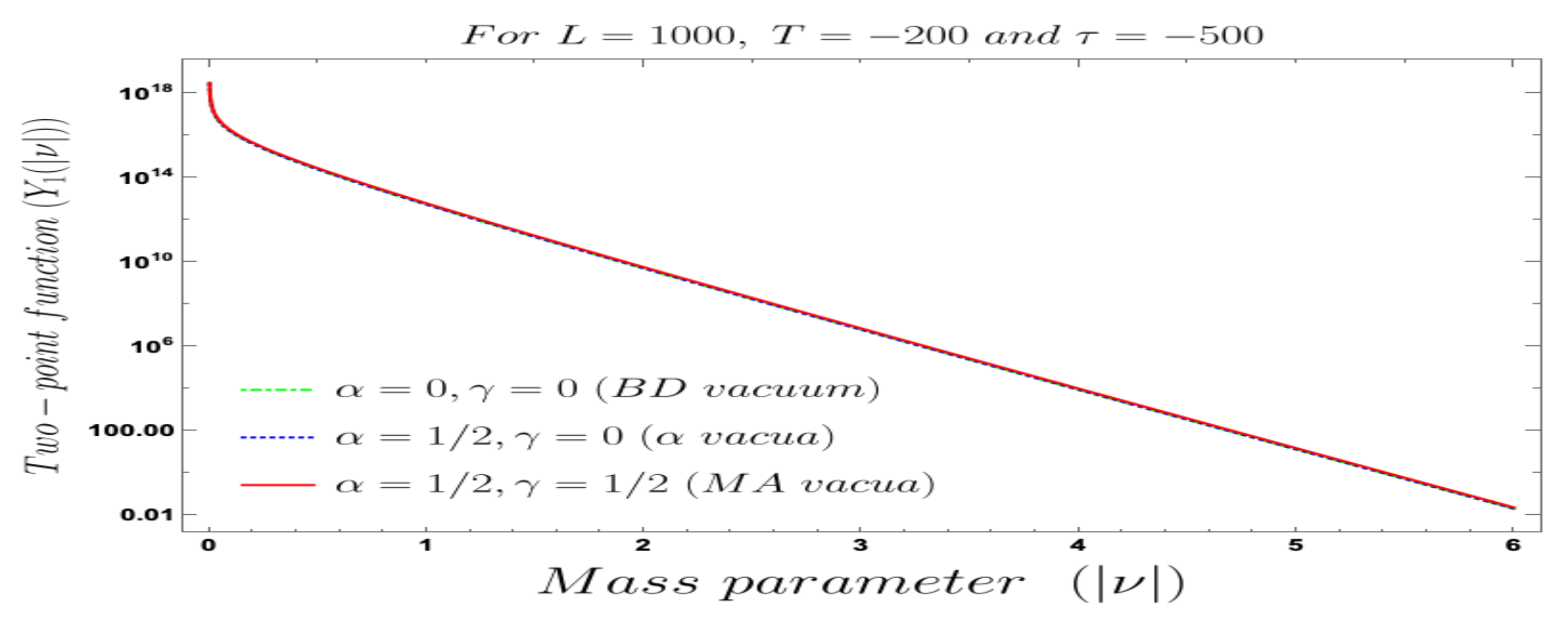
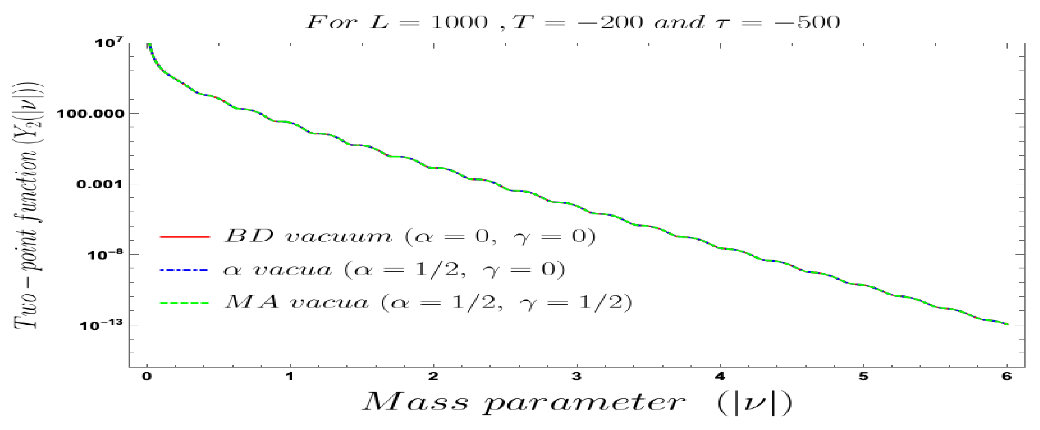
• In the presence of a very heavy mass particle, which is within the framework of cosmology and identified by the limiting situation, $m\gg H$, where H is the characteristic Hubble scale, one needs to take the analytical continuation of the mass parameter $\nu$ to the imaginary axis such that, $\nu \to -\left|\nu \right|$. As a consequence of this we get a exponential Boltzmann suppression by a factor of $exp(-2|\nu \left|\pi \right)$, which can be treated as a correction term in the final expressions for the two-point OTOCs. Now, if the magnitude of the mass parameter $\left|\nu \right|$ is extremely large then one can simply drop this exponential Boltzmann factor in the final expression for the two-point OTOCs and can be written as:

  $$\begin{array}{c}\hfill Large\left|\nu \right|\left(\right|\nu |\to \infty )approximation:\end{array}$$

  $$\begin{array}{c}\hfill Y_1^f({\tau }_1,{\tau }_2)\approx \frac{{\mathcal{H}}_1({\tau }_1,{\tau }_2,\left|\nu \right|)}{2{\pi }^2}{\nabla }_{32}^{\left(1\right)}({\tau }_1,{\tau }_2).\end{array}$$

  (273)

  $$\begin{array}{c}\hfill Y_2^f({\tau }_1,{\tau }_2)\approx \frac{{\mathcal{H}}_2({\tau }_1,{\tau }_2,\left|\nu \right|)}{2{\pi }^2}{\nabla }_{32}^{\left(2\right)}({\tau }_1,{\tau }_2),\end{array}$$

  (274)

  $$\begin{array}{c}\hfill Y_1^{\zeta }({\tau }_1,{\tau }_2)\approx \frac{{\mathcal{H}}_1({\tau }_1,{\tau }_2,\left|\nu \right|)}{2{\pi }^{2}z\left({\tau }_1\right)z\left({\tau }_2\right)}{\nabla }_{32}^{\left(1\right)}({\tau }_1,{\tau }_2).\end{array}$$

  (275)

  $$\begin{array}{c}\hfill Y_2^{\zeta }({\tau }_1,{\tau }_2)\approx \frac{{\mathcal{H}}_2({\tau }_1,{\tau }_2,\left|\nu \right|)}{2{\pi }^{2}z\left({\tau }_1\right)z\left({\tau }_2\right)}{\nabla }_{32}^{\left(2\right)}({\tau }_1,{\tau }_2),\end{array}$$

  (276)

  where we define new functions ${\mathcal{H}}_1({\tau }_1,{\tau }_2,\left|\nu \right|)$ and ${\mathcal{H}}_2({\tau }_1,{\tau }_2,\left|\nu \right|)$, which are given by:

  $$\begin{array}{ccc}& & {\mathcal{H}}_1({\tau }_1,{\tau }_2,\left|\nu \right|):\equiv {(-{\tau }_1)}^{i\left|\nu \right|}{(-{\tau }_2)}^{i\left|\nu \right|}\left(1+\frac{1}{2}ln(-{\tau }_1)\right)\left(1+\frac{1}{2}ln(-{\tau }_2)\right),\hfill \end{array}$$

  (277)

  $$\begin{array}{ccc}& & {\mathcal{H}}_2({\tau }_1,{\tau }_2,\left|\nu \right|):\equiv {(-{\tau }_1)}^{i\left|\nu \right|}{(-{\tau }_2)}^{i\left|\nu \right|}\left(1+\frac{3}{2}ln(-{\tau }_1)\right)\left(1+\frac{3}{2}ln(-{\tau }_2)\right),\hfill \end{array}$$

  (278)
  Here, it is important to note that to define this function we have used the following expansion:

  $$\begin{array}{ccc}& & {\left(-{\tau }_k\right)}^{{\delta }_j+i\left|\nu \right|}\approx {\left(-{\tau }_j\right)}^{i\left|\nu \right|}\left[1+{\delta }_{j}ln(-{\tau }_j)+\cdots \right],\forall k=1,2\&j=1,2(k\ne j)\hfill \\ & & ‘\mathrm{with}{\delta }_1=\frac{1}{2},{\delta }_2=\frac{3}{2},\hfill \end{array}$$

  (279)

  where we have considered the fact that, $\left|\nu \right|\gg {\delta }_j\forall j=1,2$ and $\left|\nu \right|\to \infty$ to get the leading and the sub-leading or the next to leading order contribution, which is used for the further simplification of the obtained result for the two-point OTOC in the large $\left|\nu \right|$ limit. We also have introduced the following symbolic representation for the sake of simplicity and clarity:

  $$\begin{array}{c}\hfill {\nabla }_{32}^{\left(i\right)}({\tau }_1,{\tau }_2):\equiv \underset{\left|\nu \right|\to \infty }{lim}\left({\mathcal{Z}}_{\left(3\right)}^{\left(i\right)}({\tau }_1,{\tau }_2)-{\mathcal{Z}}_{\left(2\right)}^{\left(i\right)}({\tau }_1,{\tau }_2)\right)\forall i=1,2.\end{array}$$

  (280)
  On the other hand, if the magnitude of the mass parameter is small then one can expand the exponential Boltzmann factor in the Taylor series and keep up to the linear order term in $\nu$ in the expansion. This will give rise to an overall contribution, which is given by $2\left(1-\left|\nu \right|\pi \right)$ and the corresponding two-point OTOCs can be approximately written as:

  $$\begin{array}{c}\hfill Small\left|\nu \right|\left(\right|\nu |\to 0)approximation:\end{array}$$

  $$\begin{array}{c}\hfill Y_1^f({\tau }_1,{\tau }_2)=\frac{{\mathcal{T}}_1({\tau }_1,{\tau }_2,\left|\nu \right|)}{2{\pi }^2}{\Delta }_{32}^{\left(1\right)}({\tau }_1,{\tau }_2).\end{array}$$

  (281)

  $$\begin{array}{c}\hfill Y_2^f({\tau }_1,{\tau }_2)=\frac{{\mathcal{T}}_2({\tau }_1,{\tau }_2,\left|\nu \right|)}{2{\pi }^2}{\Delta }_{32}^{\left(2\right)}({\tau }_1,{\tau }_2),\end{array}$$

  (282)

  $$\begin{array}{c}\hfill Y_1^{\zeta }({\tau }_1,{\tau }_2)=\frac{{\mathcal{T}}_1({\tau }_1,{\tau }_2,\left|\nu \right|)}{2{\pi }^{2}z\left({\tau }_1\right)z\left({\tau }_2\right)}{\Delta }_{32}^{\left(1\right)}({\tau }_1,{\tau }_2).\end{array}$$

  (283)

  $$\begin{array}{c}\hfill Y_2^{\zeta }({\tau }_1,{\tau }_2)=\frac{{\mathcal{T}}_2({\tau }_1,{\tau }_2,\left|\nu \right|)}{2{\pi }^{2}z\left({\tau }_1\right)z\left({\tau }_2\right)}{\Delta }_{32}^{\left(2\right)}({\tau }_1,{\tau }_2),\end{array}$$

  (284)

  where we define new functions ${\mathcal{T}}_1({\tau }_1,{\tau }_2,\left|\nu \right|)$ and ${\mathcal{T}}_2({\tau }_1,{\tau }_2,\left|\nu \right|)$, which are given by:

  $$\begin{array}{ccc}& & {\mathcal{T}}_1({\tau }_1,{\tau }_2,\left|\nu \right|):\equiv {(-{\tau }_1)}^{\frac{1}{2}}{(-{\tau }_2)}^{\frac{1}{2}}\left(1+i\left|\nu \right|ln(-{\tau }_1)\right)\left(1+i\left|\nu \right|ln(-{\tau }_2)\right)\left(1-\left|\nu \right|\pi \right),\hfill \end{array}$$

  (285)

  $$\begin{array}{ccc}& & {\mathcal{T}}_2({\tau }_1,{\tau }_2,\left|\nu \right|):\equiv {(-{\tau }_1)}^{\frac{3}{2}}{(-{\tau }_2)}^{\frac{3}{2}}\left(1+i\left|\nu \right|ln(-{\tau }_1)\right)\left(1+i\left|\nu \right|ln(-{\tau }_2)\right)\left(1-\left|\nu \right|\pi \right).\hfill \end{array}$$

  (286)
  Here, it is important to note that to define this function we have used the following expansion:

  $$\begin{array}{ccc}& & {\left(-{\tau }_k\right)}^{{\delta }_j+i\left|\nu \right|}\approx 2{\left(-{\tau }_k\right)}^{{\delta }_j}\left[1+i\left|\nu \right|ln(-{\tau }_j)+\cdots \right],\forall j=1,2\&k=1,2(j\ne k)\hfill \\ & & ‘\mathrm{with}{\delta }_1=\frac{1}{2},{\delta }_2=\frac{3}{2},\hfill \end{array}$$

  (287)

  where we have considered the fact that ${\delta }_j\gg \left|\nu \right|\forall j=1,2$ and $\left|\nu \right|\to 0$ to get the leading and the sub-leading or the next to leading order contribution, which is used for the further simplification of the obtained result for the two-point OTOC in the small $\left|\nu \right|$ limit.
  We also have introduced the following symbolic representation for the sake of simplicity and clarity:

  $$\begin{array}{c}\hfill {\Delta }_{32}^{\left(i\right)}({\tau }_1,{\tau }_2):\equiv \underset{\left|\nu \right|\to 0}{lim}\left({\mathcal{Z}}_{\left(3\right)}^{\left(i\right)}({\tau }_1,{\tau }_2)-{\mathcal{Z}}_{\left(2\right)}^{\left(i\right)}({\tau }_1,{\tau }_2)\right)\forall i=1,2.\end{array}$$

  (288)
• One can also consider various important cases, described by the mass parameter values $\nu =0$, $\nu =3/2$ and $\nu =1/2$. Here $\nu =3/2$ represents the massless field limiting situation and $\nu =1/2$ representing the conformally coupled case, where we have $m_{\varphi }=\sqrt{2}H$. On the other hand, $\nu =0$ represents the situation where we have $m_{\varphi }=3H/2$. Here, one can treat both $\nu =0$ and $\nu =1/2$ in the partially massless field category.
• We have explicitly shown that the two-point OTOCs defined in this work are completely independent of the choice of the coordinate system and at the end only depend on the time scale on which the cosmologically relevant operators in perturbation theory are separated in time scale. To define properly, we define these operators in terms of a specific space coordinate point but at different time scales and found that the final answer of the two-point OTOCs are only dependent on time scale.
• From the present computation we found that the final expression for the two-point OTOCs are completely independent on temperature even though we start with a thermal canonical statistical ensemble in the trace formula of the two-point OTOCs. It implies that we will get ultimately the description in terms of statistical ensembles following the present description within the framework of cosmological perturbation theory, which is obviously a quite interesting observation to point out in the present context of computation.
• Now if we fix the conformal time coordinate of the two operators, ${\tau }_1=\tau$ and ${\tau }_2=\tau$, that means if both the cosmologically relevant operators are defined at the same time coordinate (time separation vanishes) then two-point OTOCs show divergence. On the other hand, if we compare the obtained result with the expression for any two-point equal time cosmological correlators of the perturbation field variables then the amplitude of such correlators, which we commonly identified to be the power spectrum within the framework of cosmology, are found to be finite. Therefore, this observation implies that just by converting OTOC to ETOC one cannot get a correct and finite answer. This is because of the fact that OTOC deals with completely out-of-equilibrium phenomena and ETOC deals with completely equal phenomena. It is expected that after taking a very large late time limit, it is possible to achieve equilibrium in any one of the time coordinates involved in the cosmological operators, but to get a complete equilibrium description in ETOC one needs to follow a completely different approach starting from the definition.
• After doing simple computation, one can explicitly show that, in the present context, the one-point and three-point functions are explicitly zero and can be written as:

  $$\begin{array}{ccc}& & {\langle \hat{f}(\mathbf{x},\tau )\rangle }_{\beta }=\frac{1}{Z(\beta ;\tau )}\mathrm{Tr}\left[e^{-\beta \hat{H}\left(\tau \right)}\hat{f}(\mathbf{x},\tau )\right]=0,\hfill \end{array}$$

  (289)

  $$\begin{array}{ccc}& & {\langle \hat{\mathsf{\Pi }}(\mathbf{x},\tau )\rangle }_{\beta }=\frac{1}{Z(\beta ;\tau )}\mathrm{Tr}\left[e^{-\beta \hat{H}\left(\tau \right)}\hat{\mathsf{\Pi }}(\mathbf{x},\tau )\right]=0.\hfill \end{array}$$

  (290)

  $$\begin{array}{ccc}& & {\langle \hat{f}(\mathbf{x},{\tau }_1)\hat{f}(\mathbf{x},{\tau }_2)\hat{f}(\mathbf{x},{\tau }_3)\rangle }_{\beta }=\frac{1}{Z(\beta ;\tau )}\mathrm{Tr}\left[e^{-\beta \hat{H}\left(\tau \right)}\hat{f}(\mathbf{x},\tau )\hat{f}(\mathbf{x},{\tau }_2)\hat{f}(\mathbf{x},{\tau }_3)\right]=0,\hfill \end{array}$$

  (291)

  $$\begin{array}{ccc}& & {\langle \hat{\mathsf{\Pi }}(\mathbf{x},{\tau }_1)\hat{\mathsf{\Pi }}(\mathbf{x},{\tau }_2)\hat{\mathsf{\Pi }}(\mathbf{x},{\tau }_3)\rangle }_{\beta }=\frac{1}{Z(\beta ;\tau )}\mathrm{Tr}\left[e^{-\beta \hat{H}\left(\tau \right)}\hat{\mathsf{\Pi }}(\mathbf{x},{\tau }_1)\hat{\mathsf{\Pi }}(\mathbf{x},{\tau }_2)\hat{\mathsf{\Pi }}(\mathbf{x},{\tau }_3)\right]=0.\hfill \end{array}$$

  (292)
  Here, we have used the well-known Kubo Martin Schwinger condition, which basically deals with the time translational symmetry at finite temperature and using this fact one can explicitly show that the above two combinations of the three point function for the cosmological perturbation theory explicitly vanishes in the present context. Not only these combinations, but also the other possible cross correlated three-point function will become similarly zero. If we do the computation for the primordial cosmological scalar perturbations explicitly in zero temperature then one can explicitly find non-zero but small answers for all the possible three-point correlators using the concept of OTOC. Using the Kubo–Martin–Schwinger condition, one can further show that for any odd N-point function at finite temperature the corresponding contribution vanishes due to the time translational symmetry. For these mentioned reasons OTOCs are not defined in terms of any odd N-point function within the framework of out-of-equilibrium quantum field theory. All even N-point OTOCs are normalised with appropriate factors which actually appear from the expansion in the large time dissipation time scale $t\sim \beta =T^{-1}$, which is basically proportional to the equilibrium temperature of the quantum system under consideration at very late time limit. On the other hand, since one cannot decompose the odd N-point thermal correlators in symmetric combinations and each correlator is trivially zero there is no normalisation possible to express these correlators. Therefore, the only physical information is appearing from all even N-point correlators. For $N=2$ we get the two-point OTOCs which we do not need to normalise because in this computation these are treated as the smallest building block for the computation. Any other even $N>2$-point correlators can be normalised in terms of the combinations of the $N=2$ point disconnected part of the OTOCs which are basically appearing in the large time dissipation time scale as previously we have mentioned. In our previous paper [53], we have provided the detailed computation of a specific type of two-point and four-point OTOC out of which one is able to extract various unknown physical information within the framework of cosmological perturbation theory described in the out-of-equilibrium regime of quantum field theory. In this paper we actually go beyond this understanding of the OTOC and can provide two new sets of two-point and four-point OTOCs which we believe can give other information regarding the quantum system under study within the framework of cosmological perturbation theory in the out of equilibrium regime of the quantum field theory. In the next subsections, we are going to provide the detailed computations of the “in-in” OTO amplitudes and the related four-point OTOCs from the primordial scalar perturbations.

3.10. Trace of Four-Point “In-In” Non-Chaotic Auto-Correlated OTO Amplitude for Primordial Cosmology

Now, we will explicitly compute the numerator of the first type of four-point OTOC constructed out of cosmological perturbation field variable for different quantum vacuum states, which is given by:

$$\begin{array}{ccc}& & \mathrm{Tr}{\left[e^{-\beta \hat{H}\left({\tau }_1\right)}{\left[\hat{f}(\mathbf{x},{\tau }_1),\hat{f}(\mathbf{x},{\tau }_2)\right]}^2\right]}_{(\alpha ,\gamma )}\hfill \\ & & =\frac{exp(-2sin\gamma tan\alpha )}{|cosh\alpha |}\int d{\Psi }_{\mathbf{BD}}\prod _{j=1}^4\int \frac{d^3{k}_j}{{\left(2\pi \right)}^3}exp\left[i{\mathbf{k}}_j.\mathbf{x}\right]\hfill \\ & & \langle {\Psi }_{\mathbf{BD}}|\left[{\displaystyle \sum _{i=1}^4}{\widehat{\mathcal{V}}}_i^{\left(1\right)}({\mathbf{k}}_1,{\mathbf{k}}_2,{\mathbf{k}}_3,{\mathbf{k}}_4;{\tau }_1,{\tau }_2;\beta )\right]|{\Psi }_{\mathbf{BD}}\rangle .\hfill \end{array}$$

(293)

On the other hand, we will explicitly compute the numerator of the second type of four-point OTOC constructed out of cosmological perturbation field momenta variable for different quantum vacuum states, which is given by:

$$\begin{array}{ccc}& & \mathrm{Tr}{\left[e^{-\beta \hat{H}\left({\tau }_1\right)}{\left[\hat{\mathsf{\Pi }}(\mathbf{x},{\tau }_1),\hat{\mathsf{\Pi }}(\mathbf{x},{\tau }_2)\right]}^2\right]}_{(\alpha ,\gamma )}\hfill \\ & & =\frac{exp(-2sin\gamma tan\alpha )}{|cosh\alpha |}\int d{\Psi }_{\mathbf{BD}}\prod _{j=1}^4\int \frac{d^3{k}_j}{{\left(2\pi \right)}^3}exp\left[i{\mathbf{k}}_j.\mathbf{x}\right]\hfill \\ & & \langle {\Psi }_{\mathbf{BD}}|\left[{\displaystyle \sum _{i=1}^4}{\widehat{\mathcal{V}}}_i^{\left(2\right)}({\mathbf{k}}_1,{\mathbf{k}}_2,{\mathbf{k}}_3,{\mathbf{k}}_4;{\tau }_1,{\tau }_2;\beta )\right]|{\Psi }_{\mathbf{BD}}\rangle .\hfill \end{array}$$

(294)

Further, our aim is to compute the individual contributions which in the normal ordered form are given by the following expression and are explicitly computed in the Appendix of this paper:

$$\begin{array}{ccc}& & \int d{\Psi }_{\mathbf{BD}}\langle {\Psi }_{\mathbf{BD}}|:{\widehat{\mathcal{V}}}_i^{\left(1\right)}({\mathbf{k}}_1,{\mathbf{k}}_2,{\mathbf{k}}_3,{\mathbf{k}}_4;{\tau }_1,{\tau }_2;\beta ):|{\Psi }_{\mathbf{BD}}\rangle \hfill \\ & & =\int d{\Psi }_{\mathbf{BD}}\langle {\Psi }_{\mathbf{BD}}|:e^{-\beta \hat{H}\left({\tau }_1\right)}{\widehat{\mathcal{T}}}_i^{\left(1\right)}({\mathbf{k}}_1,{\mathbf{k}}_2,{\mathbf{k}}_3,{\mathbf{k}}_4;{\tau }_1,{\tau }_2):|{\Psi }_{\mathbf{BD}}\rangle ,\hfill \end{array}$$

(295)

$$\begin{array}{ccc}& & \int d{\Psi }_{\mathbf{BD}}\langle {\Psi }_{\mathbf{BD}}|:{\widehat{\mathcal{V}}}_i^{\left(2\right)}({\mathbf{k}}_1,{\mathbf{k}}_2,{\mathbf{k}}_3,{\mathbf{k}}_4;{\tau }_1,{\tau }_2;\beta ):|{\Psi }_{\mathbf{BD}}\rangle \hfill \\ & & =\int d{\Psi }_{\mathbf{BD}}\langle {\Psi }_{\mathbf{BD}}|:e^{-\beta \hat{H}\left({\tau }_1\right)}{\widehat{\mathcal{T}}}_i^{\left(2\right)}({\mathbf{k}}_1,{\mathbf{k}}_2,{\mathbf{k}}_3,{\mathbf{k}}_4;{\tau }_1,{\tau }_2):|{\Psi }_{\mathbf{BD}}\rangle \forall i=1,2,3,4.\hfill \end{array}$$

(296)

Here, it is important to note that the dispersion relation in general has to be different for different choices of the initial quantum vacuum state.

3.11. New OTOCs from Regularised Four-Point “In-In” Non-Chaotic Auto-Correlated OTO Amplitudes: Rescaled Field Version

3.11.1. Without Normalisation

The desired cosmological OTOCs without normalisation can be expressed as:

$$\begin{array}{ccc}& & C_1^f({\tau }_1,{\tau }_2)=-\frac{1}{Z(\beta ;{\tau }_1)}\mathrm{Tr}\left[e^{-\beta \hat{H}\left({\tau }_1\right)}{\left[\hat{f}(\mathbf{x},{\tau }_1),\hat{f}(\mathbf{x},{\tau }_2)\right]}^2\right]\hfill \\ & & =-\int \frac{d^3{k}_1}{{\left(2\pi \right)}^3}\int \frac{d^3{k}_2}{{\left(2\pi \right)}^3}\left\{{\mathcal{E}}_4^{\left(1\right)}({\mathbf{k}}_1,{\mathbf{k}}_2,-{\mathbf{k}}_2,-{\mathbf{k}}_1;{\tau }_1,{\tau }_2)+{\mathcal{E}}_4^{\left(1\right)}({\mathbf{k}}_1,{\mathbf{k}}_2,-{\mathbf{k}}_1,-{\mathbf{k}}_2;{\tau }_1,{\tau }_2)\right.\hfill \\ & & +{\mathcal{E}}_6^{\left(1\right)}({\mathbf{k}}_1,{\mathbf{k}}_2,-{\mathbf{k}}_2,-{\mathbf{k}}_1;{\tau }_1,{\tau }_2)+{\mathcal{E}}_7^{\left(1\right)}({\mathbf{k}}_1,{\mathbf{k}}_2,-{\mathbf{k}}_1,-{\mathbf{k}}_2;{\tau }_1,{\tau }_2)\hfill \\ & & +{\mathcal{E}}_{10}^{\left(1\right)}({\mathbf{k}}_1,{\mathbf{k}}_2,-{\mathbf{k}}_1,-{\mathbf{k}}_2;{\tau }_1,{\tau }_2)+{\mathcal{E}}_{11}^{\left(1\right)}({\mathbf{k}}_1,{\mathbf{k}}_2,-{\mathbf{k}}_2,-{\mathbf{k}}_1;{\tau }_1,{\tau }_2)\hfill \\ & & +{\mathcal{E}}_{13}^{\left(1\right)}({\mathbf{k}}_1,{\mathbf{k}}_2,-{\mathbf{k}}_1,-{\mathbf{k}}_2;{\tau }_1,{\tau }_2)+{\mathcal{E}}_{13}^{\left(1\right)}({\mathbf{k}}_1,{\mathbf{k}}_2,-{\mathbf{k}}_2,-{\mathbf{k}}_1;{\tau }_1,{\tau }_2)\hfill \\ & & \left.+{\mathcal{E}}_7^{\left(1\right)}({\mathbf{k}}_1,-{\mathbf{k}}_1,{\mathbf{k}}_2,-{\mathbf{k}}_2;{\tau }_1,{\tau }_2)+{\mathcal{E}}_{10}^{\left(1\right)}({\mathbf{k}}_1,-{\mathbf{k}}_1,{\mathbf{k}}_2,-{\mathbf{k}}_2;{\tau }_1,{\tau }_2)+{\mathcal{E}}_{11}^{\left(1\right)}({\mathbf{k}}_1,-{\mathbf{k}}_1,{\mathbf{k}}_2,-{\mathbf{k}}_2;{\tau }_1,{\tau }_2)\right\},\hfill \end{array}$$

(297)

$$\begin{array}{ccc}& & C_2^f({\tau }_1,{\tau }_2)=-\frac{1}{Z(\beta ;{\tau }_1)}\mathrm{Tr}\left[e^{-\beta \hat{H}\left({\tau }_1\right)}{\left[\widehat{\mathsf{\Pi }}(\mathbf{x},{\tau }_1),\hat{\mathsf{\Pi }}(\mathbf{x},{\tau }_2)\right]}^2\right]\hfill \\ & & =-\int \frac{d^3{k}_1}{{\left(2\pi \right)}^3}\int \frac{d^3{k}_2}{{\left(2\pi \right)}^3}\left\{{\mathcal{E}}_4^{\left(2\right)}({\mathbf{k}}_1,{\mathbf{k}}_2,-{\mathbf{k}}_2,-{\mathbf{k}}_1;{\tau }_1,{\tau }_2)+{\mathcal{E}}_4^{\left(2\right)}({\mathbf{k}}_1,{\mathbf{k}}_2,-{\mathbf{k}}_1,-{\mathbf{k}}_2;{\tau }_1,{\tau }_2)\right.\hfill \\ & & +{\mathcal{E}}_6^{\left(2\right)}({\mathbf{k}}_1,{\mathbf{k}}_2,-{\mathbf{k}}_2,-{\mathbf{k}}_1;{\tau }_1,{\tau }_2)+{\mathcal{E}}_7^{\left(2\right)}({\mathbf{k}}_1,{\mathbf{k}}_2,-{\mathbf{k}}_1,-{\mathbf{k}}_2;{\tau }_1,{\tau }_2)\hfill \\ & & +{\mathcal{E}}_{10}^{\left(2\right)}({\mathbf{k}}_1,{\mathbf{k}}_2,-{\mathbf{k}}_1,-{\mathbf{k}}_2;{\tau }_1,{\tau }_2)+{\mathcal{E}}_{11}^{\left(2\right)}({\mathbf{k}}_1,{\mathbf{k}}_2,-{\mathbf{k}}_2,-{\mathbf{k}}_1;{\tau }_1,{\tau }_2)\hfill \\ & & +{\mathcal{E}}_{13}^{\left(2\right)}({\mathbf{k}}_1,{\mathbf{k}}_2,-{\mathbf{k}}_1,-{\mathbf{k}}_2;{\tau }_1,{\tau }_2)+{\mathcal{E}}_{13}^{\left(2\right)}({\mathbf{k}}_1,{\mathbf{k}}_2,-{\mathbf{k}}_2,-{\mathbf{k}}_1;{\tau }_1,{\tau }_2)\hfill \\ & & \left.+{\mathcal{E}}_7^{\left(2\right)}({\mathbf{k}}_1,-{\mathbf{k}}_1,{\mathbf{k}}_2,-{\mathbf{k}}_2;{\tau }_1,{\tau }_2)+{\mathcal{E}}_{10}^{\left(2\right)}({\mathbf{k}}_1,-{\mathbf{k}}_1,{\mathbf{k}}_2,-{\mathbf{k}}_2;{\tau }_1,{\tau }_2)+{\mathcal{E}}_{11}^{\left(2\right)}({\mathbf{k}}_1,-{\mathbf{k}}_1,{\mathbf{k}}_2,-{\mathbf{k}}_2;{\tau }_1,{\tau }_2)\right\},\hfill \end{array}$$

(298)

where we have introduced new four-point OTO amplitude functions, ${\mathcal{E}}_m^{\left(1\right)},{\mathcal{E}}_m^{\left(2\right)}\forall m=4,6,7,10,11,13$, which are defined as:

$$\begin{array}{ccc}\hfill {\mathcal{E}}_m^{\left(l\right)}({\mathbf{k}}_1,{\mathbf{k}}_2,{\mathbf{k}}_3,{\mathbf{k}}_4;{\tau }_1,{\tau }_2)& =& {\mathcal{M}}_m^{\left(l\right)}-{\mathcal{J}}_m^{\left(l\right)}+{\mathcal{N}}_m^{\left(l\right)}-{\mathcal{Q}}_m^{\left(l\right)}\forall l=1,2,\hfill \end{array}$$

(299)

All these functions signify the amplitude of the desired two types of OTOCs which are expressed in terms of the contributions from the four-point functions. For further simplification, we have to consider symmetry properties of the above-mentioned amplitudes under the exchange of the momenta appearing in the third and fourth position, i.e., if we replace $-{\mathbf{k}}_2\to -{\mathbf{k}}_1$ and $-{\mathbf{k}}_1\to -{\mathbf{k}}_2$, which are given by the following expressions:

$$\begin{array}{c}\hfill {\mathcal{E}}_4^{\left(l\right)}({\mathbf{k}}_1,{\mathbf{k}}_2,-{\mathbf{k}}_2,-{\mathbf{k}}_1;{\tau }_1,{\tau }_2)={\mathcal{E}}_4^{\left(l\right)}({\mathbf{k}}_1,{\mathbf{k}}_2,-{\mathbf{k}}_1,-{\mathbf{k}}_2;{\tau }_1,{\tau }_2)\forall l=1,2,\end{array}$$

(300)

$$\begin{array}{c}\hfill {\mathcal{E}}_{13}^{\left(l\right)}({\mathbf{k}}_1,{\mathbf{k}}_2,-{\mathbf{k}}_2,-{\mathbf{k}}_1;{\tau }_1,{\tau }_2)={\mathcal{E}}_{13}^{\left(l\right)}({\mathbf{k}}_1,{\mathbf{k}}_2,-{\mathbf{k}}_1,-{\mathbf{k}}_2;{\tau }_1,{\tau }_2)\forall l=1,2.\end{array}$$

(301)

Using these exchange symmetry properties, the desired OTOCs one can further simplify the results as:

$$\begin{array}{ccc}& & C_l^f({\tau }_1,{\tau }_2)=-\int \frac{d^3{\mathbf{k}}_1}{{\left(2\pi \right)}^3}\int \frac{d^3{\mathbf{k}}_2}{{\left(2\pi \right)}^3}\left\{2\left({\mathcal{E}}_4^{\left(l\right)}({\mathbf{k}}_1,{\mathbf{k}}_2,-{\mathbf{k}}_2,-{\mathbf{k}}_1;{\tau }_1,{\tau }_2)+{\mathcal{E}}_{13}^{\left(l\right)}({\mathbf{k}}_1,{\mathbf{k}}_2,-{\mathbf{k}}_1,-{\mathbf{k}}_2;{\tau }_1,{\tau }_2)\right)\right.\hfill \\ & & +{\mathcal{E}}_6^{\left(l\right)}({\mathbf{k}}_1,{\mathbf{k}}_2,-{\mathbf{k}}_2,-{\mathbf{k}}_1;{\tau }_1,{\tau }_2)+{\mathcal{E}}_7^{\left(l\right)}({\mathbf{k}}_1,{\mathbf{k}}_2,-{\mathbf{k}}_1,-{\mathbf{k}}_2;{\tau }_1,{\tau }_2)\hfill \\ & & +{\mathcal{E}}_{10}^{\left(l\right)}({\mathbf{k}}_1,{\mathbf{k}}_2,-{\mathbf{k}}_1,-{\mathbf{k}}_2;{\tau }_1,{\tau }_2)+{\mathcal{E}}_{11}^{\left(l\right)}({\mathbf{k}}_1,{\mathbf{k}}_2,-{\mathbf{k}}_2,-{\mathbf{k}}_1;{\tau }_1,{\tau }_2)\hfill \\ & & \left.+{\mathcal{E}}_7^{\left(l\right)}({\mathbf{k}}_1,-{\mathbf{k}}_1,{\mathbf{k}}_2,-{\mathbf{k}}_2;{\tau }_1,{\tau }_2)+{\mathcal{E}}_{10}^{\left(l\right)}({\mathbf{k}}_1,-{\mathbf{k}}_1,{\mathbf{k}}_2,-{\mathbf{k}}_2;{\tau }_1,{\tau }_2)+{\mathcal{E}}_{11}^{\left(l\right)}({\mathbf{k}}_1,-{\mathbf{k}}_1,{\mathbf{k}}_2,-{\mathbf{k}}_2;{\tau }_1,{\tau }_2)\right\}\hfill \\ & & \forall l=1,2.\hfill \end{array}$$

(302)

In this computation, the volume elements of the momentum integrals are given by the following expression:

$$\begin{array}{ccc}& & {\displaystyle \prod _{i=1}^2\frac{d^3{\mathbf{k}}_i}{{\left(2\pi \right)}^6}=\frac{1}{{\left(2\pi \right)}^6}\prod _{i=1}^2{k}_i^{2}d{k}_{i}sin{\theta }_{i}d{\theta }_{i}d{\varphi }_i,}\hfill \\ & & \mathrm{where}0<k_i<\infty ,0<{\theta }_i<\pi ,0<{\varphi }_i<2\pi \forall i=1,2.\hfill \end{array}$$

(303)

Here we need to put cut-off $0<k_i<L\forall i=1,2$ to regulate the only magnitude of the momentum-dependent radial integral and consequently we can write the following regulated expressions for the desired OTOCs, as given by:

$$\begin{array}{ccc}& & C_l^f({\tau }_1,{\tau }_2)=-\frac{1}{4{\pi }^4}{\int }_0^L{k}_1^{2}d{k}_1{\int }_0^L{k}_2^{2}d{k}_2\hfill \\ & & \left\{2\left({\mathcal{E}}_4^{\left(l\right)}({\mathbf{k}}_1,{\mathbf{k}}_2,-{\mathbf{k}}_2,-{\mathbf{k}}_1;{\tau }_1,{\tau }_2)+{\mathcal{E}}_{13}^{\left(l\right)}({\mathbf{k}}_1,{\mathbf{k}}_2,-{\mathbf{k}}_1,-{\mathbf{k}}_2;{\tau }_1,{\tau }_2)\right)\right.\hfill \\ & & +{\mathcal{E}}_6^{\left(l\right)}({\mathbf{k}}_1,{\mathbf{k}}_2,-{\mathbf{k}}_2,-{\mathbf{k}}_1;{\tau }_1,{\tau }_2)+{\mathcal{E}}_7^{\left(l\right)}({\mathbf{k}}_1,{\mathbf{k}}_2,-{\mathbf{k}}_1,-{\mathbf{k}}_2;{\tau }_1,{\tau }_2)\hfill \\ & & +{\mathcal{E}}_{10}^{\left(l\right)}({\mathbf{k}}_1,{\mathbf{k}}_2,-{\mathbf{k}}_1,-{\mathbf{k}}_2;{\tau }_1,{\tau }_2)+{\mathcal{E}}_{11}^{\left(l\right)}({\mathbf{k}}_1,{\mathbf{k}}_2,-{\mathbf{k}}_2,-{\mathbf{k}}_1;{\tau }_1,{\tau }_2)\hfill \\ & & \left.+{\mathcal{E}}_7^{\left(l\right)}({\mathbf{k}}_1,-{\mathbf{k}}_1,{\mathbf{k}}_2,-{\mathbf{k}}_2;{\tau }_1,{\tau }_2)+{\mathcal{E}}_{10}^{\left(l\right)}({\mathbf{k}}_1,-{\mathbf{k}}_1,{\mathbf{k}}_2,-{\mathbf{k}}_2;{\tau }_1,{\tau }_2)+{\mathcal{E}}_{11}^{\left(l\right)}({\mathbf{k}}_1,-{\mathbf{k}}_1,{\mathbf{k}}_2,-{\mathbf{k}}_2;{\tau }_1,{\tau }_2)\right\},\hfill \\ & & \forall l=1,2.\hfill \end{array}$$

(304)

Consequently, the OTOC can be expressed in terms of the four-point time-dependent amplitudes as:

$$\begin{array}{c}\hfill C_l^f({\tau }_1,{\tau }_2)=-\frac{1}{4{\pi }^4}{\displaystyle \sum _{j=1}^7}{w}_i^{\left(l\right)}{\mathcal{I}}_j^{\left(l\right)}({\tau }_1,{\tau }_2)\forall l=1,2.\end{array}$$

(305)

See the Appendix for details, where we have computed these functions ${\mathcal{I}}_j^{\left(l\right)}({\tau }_1,{\tau }_2)\forall l=1,2$. Once we determine all of them, then the structure of the desired OTOCs, i.e., the time-dependent behaviour in the OTOC, will be fixed. Here it is important to note that the weight factors for each individual contribution are given by the following expression:

$$\begin{array}{c}\hfill w_1^{\left(l\right)}=w_2^{\left(l\right)}=2,w_j^{\left(l\right)}=1\forall j=3,4,\cdots ,9\forall l=1,2.\end{array}$$

(306)

Further, using these above-mentioned results of the integrals, the un-normalised OTOCs can be expressed as:

$$\begin{array}{c}\hfill C_1^f({\tau }_1,{\tau }_2)=\left[1+{(-1)}^{4\nu }+\frac{7}{2}{(-1)}^{2\nu }\right]\frac{{(-{\tau }_1)}^{1-2\nu }{(-{\tau }_2)}^{1-2\nu }}{2{\pi }^4{(-1)}^{4\nu -1}}{\displaystyle \sum _{i=1}^4}{X}_i^{\left(1\right),1}({\tau }_1,{\tau }_2).\end{array}$$

(307)

$$\begin{array}{c}\hfill C_2^f({\tau }_1,{\tau }_2)=\left[1+{(-1)}^{4\nu }+\frac{7}{2}{(-1)}^{2\nu }\right]\frac{{(-{\tau }_1)}^{3-2\nu }{(-{\tau }_2)}^{3-2\nu }}{2{\pi }^4{(-1)}^{4\nu -1}}{\displaystyle \sum _{i=1}^4}{X}_i^{\left(2\right),1}({\tau }_1,{\tau }_2).\end{array}$$

(308)

Here the functions $X_i^{\left(1\right),l}({\tau }_1,{\tau }_2)\forall i=1,2,3,4,\forall l=1,2$ are defined in the Appendix.

3.11.2. With Normalisation

Further, the normalisation overall factor of OTOC is given by the following expression:

$$\begin{array}{c}\hfill {\mathcal{N}}_1^f({\tau }_1,{\tau }_2)=\frac{1}{{\langle \hat{f}\left({\tau }_1\right)\hat{f}\left({\tau }_1\right)\rangle }_{\beta }{\langle \hat{f}\left({\tau }_2\right)\hat{f}\left({\tau }_2\right)\rangle }_{\beta }}=\frac{{\pi }^4}{{\mathcal{F}}_1\left({\tau }_1\right){\mathcal{F}}_1\left({\tau }_2\right)},\end{array}$$

(309)

$$\begin{array}{c}\hfill {\mathcal{N}}_2^f({\tau }_1,{\tau }_2)=\frac{1}{{\langle \hat{\mathsf{\Pi }}\left({\tau }_1\right)\hat{\mathsf{\Pi }}\left({\tau }_1\right)\rangle }_{\beta }{\langle \hat{\mathsf{\Pi }}\left({\tau }_2\right)\hat{\mathsf{\Pi }}\left({\tau }_2\right)\rangle }_{\beta }}=\frac{{\pi }^4}{{\mathcal{F}}_2\left({\tau }_1\right){\mathcal{F}}_2\left({\tau }_2\right)}.\end{array}$$

(310)

where the time-dependent functions ${\mathcal{F}}_1\left({\tau }_i\right)$ and ${\mathcal{F}}_2\left({\tau }_i\right)$ for all $i=1,2$ are defined in the Appendix explicitly. Please look into the Appendix for the detailed computation of the normalisation factor of both of the OTOCs.

Finally, the normalised OTOCs in the present context can be computed as:

$$\begin{array}{ccc}& & {\mathcal{C}}_1^f({\tau }_1,{\tau }_2)=\frac{C_1^f({\tau }_1,{\tau }_2)}{{\langle \hat{f}\left({\tau }_1\right)\hat{f}\left({\tau }_1\right)\rangle }_{\beta }{\langle \hat{f}\left({\tau }_2\right)\hat{f}\left({\tau }_2\right)\rangle }_{\beta }}\hfill \\ & & =\left[1+{(-1)}^{4\nu }+\frac{7}{2}{(-1)}^{2\nu }\right]\frac{{(-{\tau }_1)}^{1-2\nu }{(-{\tau }_2)}^{1-2\nu }}{2{(-1)}^{4\nu -1}{\mathcal{F}}_1\left({\tau }_1\right){\mathcal{F}}_1\left({\tau }_2\right)}{\displaystyle \sum _{i=1}^4}{X}_i^{\left(1\right),1}({\tau }_1,{\tau }_2),\hfill \end{array}$$

(311)

$$\begin{array}{ccc}& & {\mathcal{C}}_2^f({\tau }_1,{\tau }_2)=\frac{C_2^f({\tau }_1,{\tau }_2)}{{\langle \hat{\mathsf{\Pi }}\left({\tau }_1\right)\hat{\mathsf{\Pi }}\left({\tau }_1\right)\rangle }_{\beta }{\langle \hat{\mathsf{\Pi }}\left({\tau }_2\right)\widehat{\mathsf{\Pi }}\left({\tau }_2\right)\rangle }_{\beta }}\hfill \\ & & =\left[1+{(-1)}^{4\nu }+\frac{7}{2}{(-1)}^{2\nu }\right]\frac{{(-{\tau }_1)}^{3-2\nu }{(-{\tau }_2)}^{3-2\nu }}{2{(-1)}^{4\nu -1}{\mathcal{F}}_2\left({\tau }_1\right){\mathcal{F}}_2\left({\tau }_2\right)}{\displaystyle \sum _{i=1}^4}{X}_i^{\left(2\right),1}({\tau }_1,{\tau }_2),\hfill \end{array}$$

(312)

which is obviously a new result in the context of primordial cosmology and we are very hopeful that this result will explore various unknown physical phenomena that happened in early universe. The detailed explanation of this obtained result will be discussed in the later half of this section.

Now we will discuss about two limiting results, which are commonly known as the large mass and small mass limit of the field perturbation. Here, we will explicitly study the analytical behaviour of the two types of the derived OTOCs in the present context of discussion. This is only because of the fact that by seeing the derived expression for the complicated structure of the OTOCs one cannot comment on the features of them without numerically plotting the behaviour. The derived limiting results in this subsection will help us to understand the underlying physical features of these two types of OTOCs without explicitly performing numerical computations using the derived full results in this section.

First of all, we discuss the large mass limiting situation, which can be easily obtained by performing an explicit analytical continuation in the mass parameter $\nu$ to $-i\left|\nu \right|$. One can argue here that for this computation $\nu$ to $i\left|\nu \right|$ is not at all allowed as this will give rise to the over/excessive particle production in the four-point OTOC spectra computed in the two explicit cases that we are studying in this paper. Now, after doing the mentioned allowed analytical continuation in the mass parameter, we get the following results for the OTOCs that we can obtain in the large mass limiting case:

$$\begin{array}{ccc}& & \widetilde{{\mathcal{C}}_1^f({\tau }_1,{\tau }_2)}=\left[1+{(-1)}^{-4i\left|\nu \right|}+\frac{7}{2}{(-1)}^{-2i\left|\nu \right|}\right]\frac{{(-{\tau }_1)}^{1+2i\left|\nu \right|}{(-{\tau }_2)}^{1+2i\left|\nu \right|}}{2{(-1)}^{-\left(4i\right|\nu |+1)}\widetilde{{\mathcal{F}}_1\left({\tau }_1\right)}\widetilde{{\mathcal{F}}_1\left({\tau }_2\right)}}{\displaystyle \sum _{i=1}^4}\widetilde{X_i^{\left(1\right),1}({\tau }_1,{\tau }_2)},\hfill \end{array}$$

(313)

$$\begin{array}{ccc}& & \widetilde{{\mathcal{C}}_2^f({\tau }_1,{\tau }_2)}=\left[1+{(-1)}^{-4i\left|\nu \right|}+\frac{7}{2}{(-1)}^{-2i\left|\nu \right|}\right]\frac{{(-{\tau }_1)}^{3+2i\left|\nu \right|}{(-{\tau }_2)}^{3+2i\left|\nu \right|}}{2{(-1)}^{-\left(4i\right|\nu |+1)}\widetilde{{\mathcal{F}}_2\left({\tau }_1\right)}\widetilde{{\mathcal{F}}_2\left({\tau }_2\right)}}{\displaystyle \sum _{i=1}^4}\widetilde{X_i^{\left(2\right),1}({\tau }_1,{\tau }_2)},\hfill \end{array}$$

(314)

where $\widetilde{{\mathcal{F}}_1\left({\tau }_1\right)}$, $\widetilde{{\mathcal{F}}_1\left({\tau }_2\right)}$, $\widetilde{{\mathcal{F}}_2\left({\tau }_1\right)}$ and $\widetilde{{\mathcal{F}}_2\left({\tau }_2\right)}$ are the normalisation factors for the two OTOCs for the large mass limiting situation which is obtained by taking analytical continuation in the mass parameter $\nu$ to $-i\left|\nu \right|$. In addition, the functions $\widetilde{X_i^{\left(1\right),1}({\tau }_1,{\tau }_2)}$ and $\widetilde{X_i^{\left(2\right),1}({\tau }_1,{\tau }_2)}$ can be similarly obtained by doing the same analytical continuation in the large mass limiting situation. The explicit expressions are very cumbersome to write, therefore we have only given the expressions for these functions for the general mass parameter $\nu$. Using these expressions, by taking the above results one can explicitly compute the behaviour of these functions in the large mass limiting situation.

Furthermore, one can simplify the above-mentioned two results of the OTOCs by using the following expansion:

$$\begin{array}{ccc}& & {\left(-{\tau }_k\right)}^{{\delta }_j+i\left|\nu \right|}\approx {\left(-{\tau }_j\right)}^{i\left|\nu \right|}\left[1+{\delta }_{j}ln(-{\tau }_j)+\cdots \right],\forall k=1,2\&j=1,2(k\ne j)\hfill \\ & & ‘\mathrm{with}{\delta }_1=\frac{1}{2},{\delta }_2=\frac{3}{2},\hfill \end{array}$$

(315)

where we have considered the fact that $\left|\nu \right|\gg {\delta }_j\forall j=1,2$ and $\left|\nu \right|\to \infty$ to get the leading and the sub-leading or the next to leading order contribution, which is used for the further simplification of the obtained results for the four-point OTOCs in the large $\left|\nu \right|$ limit. Using this result, we get the following simplified results for the two types of the desired OTOCs studied in this paper:

$$\begin{array}{ccc}& & \widetilde{{\mathcal{C}}_1^f({\tau }_1,{\tau }_2)}\approx \left[1+{(-1)}^{-4i\left|\nu \right|}+\frac{7}{2}{(-1)}^{-2i\left|\nu \right|}\right]{\left(1+\frac{1}{2}ln(-{\tau }_1)\right)}^2{\left(1+\frac{1}{2}ln(-{\tau }_2)\right)}^2\hfill \\ & & \times \frac{{(-{\tau }_1)}^{2i\left|\nu \right|}{(-{\tau }_2)}^{2i\left|\nu \right|}}{2{(-1)}^{-\left(4i\right|\nu |+1)}\widetilde{{\mathcal{F}}_1\left({\tau }_1\right)}\widetilde{{\mathcal{F}}_1\left({\tau }_2\right)}}{\displaystyle \sum _{i=1}^4}\widetilde{X_i^{\left(1\right),1}({\tau }_1,{\tau }_2)},\hfill \end{array}$$

(316)

$$\begin{array}{ccc}& & \widetilde{{\mathcal{C}}_2^f({\tau }_1,{\tau }_2)}\approx \left[1+{(-1)}^{-4i\left|\nu \right|}+\frac{7}{2}{(-1)}^{-2i\left|\nu \right|}\right]{\left(1+\frac{3}{2}ln(-{\tau }_1)\right)}^2{\left(1+\frac{3}{2}ln(-{\tau }_2)\right)}^2\hfill \\ & & \times \frac{{(-{\tau }_1)}^{2i\left|\nu \right|}{(-{\tau }_2)}^{2i\left|\nu \right|}}{2{(-1)}^{-\left(4i\right|\nu |+1)}\widetilde{{\mathcal{F}}_2\left({\tau }_1\right)}\widetilde{{\mathcal{F}}_2\left({\tau }_2\right)}}{\displaystyle \sum _{i=1}^4}\widetilde{X_i^{\left(2\right),1}({\tau }_1,{\tau }_2)}.\hfill \end{array}$$

(317)

Next, we discuss the small mass limiting result for the two derived desired OTOCs in this paper. Here, we have use the following expansion for the case when the mass parameter is sufficiently small:

$$\begin{array}{ccc}& & {\left(-{\tau }_k\right)}^{{\delta }_j+i\left|\nu \right|}\approx 2{\left(-{\tau }_k\right)}^{{\delta }_j}\left[1+i\left|\nu \right|ln(-{\tau }_j)+\cdots \right],\forall j=1,2\&k=1,2(j\ne k)\hfill \\ & & ‘\mathrm{with}{\delta }_1=\frac{1}{2},{\delta }_2=\frac{3}{2},\hfill \end{array}$$

(318)

where we have considered the fact that ${\delta }_j\gg \left|\nu \right|\forall j=1,2$ and $\left|\nu \right|\to 0$ to get the leading and the sub-leading or the next to leading order contribution, which is used for the further simplification of the obtained result for the two-point OTOC in the small $\left|\nu \right|$ limit. In this limiting case, these two desired OTOCs can be further simplified as:

$$\begin{array}{ccc}& & \widehat{{\mathcal{C}}_1^f({\tau }_1,{\tau }_2)}\approx \left[1+{(-1)}^{-4i\left|\nu \right|}+\frac{7}{2}{(-1)}^{-2i\left|\nu \right|}\right]{\left(1+i\left|\nu \right|ln(-{\tau }_1)\right)}^2{\left(1+i\left|\nu \right|ln(-{\tau }_2)\right)}^2\hfill \\ & & \times \frac{8(-{\tau }_1)(-{\tau }_2)}{{(-1)}^{-\left(4i\right|\nu |+1)}\widehat{{\mathcal{F}}_1\left({\tau }_1\right)}\widehat{{\mathcal{F}}_1\left({\tau }_2\right)}}{\displaystyle \sum _{i=1}^4}\widehat{X_i^{\left(1\right),1}({\tau }_1,{\tau }_2)},\hfill \end{array}$$

(319)

$$\begin{array}{ccc}& & \widehat{{\mathcal{C}}_2^f({\tau }_1,{\tau }_2)}\approx \left[1+{(-1)}^{-4i\left|\nu \right|}+\frac{7}{2}{(-1)}^{-2i\left|\nu \right|}\right]{\left(1+i\left|\nu \right|ln(-{\tau }_1)\right)}^2{\left(1+i\left|\nu \right|ln(-{\tau }_2)\right)}^2\hfill \\ & & \times \frac{8{(-{\tau }_1)}^3{(-{\tau }_2)}^3}{{(-1)}^{-\left(4i\right|\nu |+1)}\widehat{{\mathcal{F}}_2\left({\tau }_1\right)}\widehat{{\mathcal{F}}_2\left({\tau }_2\right)}}{\displaystyle \sum _{i=1}^4}\widehat{X_i^{\left(2\right),1}({\tau }_1,{\tau }_2)}.\hfill \end{array}$$

(320)

Here, $\widehat{{\mathcal{F}}_1\left({\tau }_1\right)}$, $\widehat{{\mathcal{F}}_1\left({\tau }_2\right)}$, $\widehat{{\mathcal{F}}_2\left({\tau }_1\right)}$ and $\widehat{{\mathcal{F}}_2\left({\tau }_2\right)}$ are the normalisation factors for the two OTOCs for the small mass limiting situation, which is obtained by taking analytical continuation in the mass parameter $\nu$ to $-i\left|\nu \right|$. In addition, the functions $\widehat{X_i^{\left(1\right),1}({\tau }_1,{\tau }_2)}$ and $\widehat{X_i^{\left(2\right),1}({\tau }_1,{\tau }_2)}$ can be similarly obtained by doing the same expansion in the small mass limiting situation. The explicit expressions are very cumbersome to write, therefore we have only given the expressions for these functions for the general mass parameter $\nu$. Using these expressions, by taking the above expansions one can explicitly compute the behaviour of these functions in the small mass limiting situation.

3.12. New OTOCS from Regularised Four-Point “In-In” Non-Chaotic Auto-Correlated OTO Amplitudes: Curvature Perturbation Field Version

3.12.1. Without Normalisation

Here, we need to perform the computation for the un-normalised OTOC in terms of the scalar curvature perturbation and the canonically conjugate momentum associated with it, which we have found is given by the following simplified expression:

$$\begin{array}{ccc}& & C_1^{\zeta }({\tau }_1,{\tau }_2)=-\frac{1}{Z_{\alpha ,\gamma }^{\zeta }(\beta ,{\tau }_1)}\mathrm{Tr}{\left[e^{-\beta \hat{H}\left({\tau }_1\right)}{\left[\widehat{\zeta }(\mathbf{x},{\tau }_1),\widehat{\zeta }(\mathbf{x},{\tau }_2)\right]}^2\right]}_{(\alpha ,\gamma )}=\frac{1}{z^2\left({\tau }_1\right)z^2\left({\tau }_2\right)}{C}_1^f({\tau }_1,{\tau }_2),\hfill \end{array}$$

(321)

$$\begin{array}{ccc}& & C_2^{\zeta }({\tau }_1,{\tau }_2)=-\frac{1}{Z_{\alpha \gamma }^{\zeta }(\beta ,{\tau }_1)}\mathrm{Tr}{\left[e^{-\beta \hat{H}\left({\tau }_1\right)}{\left[\hat{\mathsf{\Pi }}(\mathbf{x},{\tau }_1),\hat{\mathsf{\Pi }}(\mathbf{x},{\tau }_2)\right]}^2\right]}_{(\alpha ,\gamma )}=\frac{1}{z^2\left({\tau }_1\right)z^2\left({\tau }_2\right)}{C}_2^f({\tau }_1,{\tau }_2).\hfill \end{array}$$

(322)

3.12.2. With Normalisation

The normalised OTOC, in terms of the scalar curvature perturbation and the canonically conjugate momentum associated with it, is basically the computation of the following normalised OTOC in the present context:

$$\begin{array}{c}\hfill {\mathcal{C}}_1^{\zeta }({\tau }_1,{\tau }_2)=\frac{C_1^{\zeta }({\tau }_1,{\tau }_2)}{{\langle \zeta \left({\tau }_1\right)\zeta \left({\tau }_1\right)\rangle }_{\beta }{\langle \zeta \left({\tau }_1\right)\zeta \left({\tau }_1\right)\rangle }_{\beta }}={\mathcal{N}}_1^{\zeta }({\tau }_1,{\tau }_2)C_1^{\zeta }({\tau }_1,{\tau }_2),\end{array}$$

(323)

$$\begin{array}{c}\hfill {\mathcal{C}}_2^{\zeta }({\tau }_1,{\tau }_2)=\frac{C_2^{\zeta }({\tau }_1,{\tau }_2)}{{\langle {\mathsf{\Pi }}_{\zeta }\left({\tau }_1\right){\mathsf{\Pi }}_{\zeta }\left({\tau }_1\right)\rangle }_{\beta }{\langle {\mathsf{\Pi }}_{\zeta }\left({\tau }_1\right){\mathsf{\Pi }}_{\zeta }\left({\tau }_1\right)\rangle }_{\beta }}={\mathcal{N}}_2^{\zeta }({\tau }_1,{\tau }_2)C_2^{\zeta }({\tau }_1,{\tau }_2),\end{array}$$

(324)

where the normalisation factor to normalise OTOC is given by:

$$\begin{array}{c}\hfill {\mathcal{N}}_1^{\zeta }({\tau }_1,{\tau }_2)=\frac{1}{{\langle \zeta \left({\tau }_1\right)\zeta \left({\tau }_1\right)\rangle }_{\beta }{\langle \zeta \left({\tau }_1\right)\zeta \left({\tau }_1\right)\rangle }_{\beta }}=\frac{{\pi }^4{z}^2\left({\tau }_1\right)z^2\left({\tau }_2\right)}{{\mathcal{F}}_1\left({\tau }_1\right){\mathcal{F}}_1\left({\tau }_2\right)}=z^2\left({\tau }_1\right)z^2\left({\tau }_2\right){\mathcal{N}}_1^f({\tau }_1,{\tau }_2),\end{array}$$

(325)

$$\begin{array}{c}\hfill {\mathcal{N}}_2^{\zeta }({\tau }_1,{\tau }_2)=\frac{1}{{\langle {\mathsf{\Pi }}_{\zeta }\left({\tau }_1\right){\mathsf{\Pi }}_{\zeta }\left({\tau }_1\right)\rangle }_{\beta }{\langle {\mathsf{\Pi }}_{\zeta }\left({\tau }_1\right){\mathsf{\Pi }}_{\zeta }\left({\tau }_1\right)\rangle }_{\beta }}=\frac{{\pi }^4{z}^2\left({\tau }_1\right)z^2\left({\tau }_2\right)}{{\mathcal{F}}_2\left({\tau }_1\right){\mathcal{F}}_2\left({\tau }_2\right)}=z^2\left({\tau }_1\right)z^2\left({\tau }_2\right){\mathcal{N}}_2^f({\tau }_1,{\tau }_2).\end{array}$$

(326)

Consequently, the normalised OTOC computed from the curvature perturbation variable is given by the following expression:

$$\begin{array}{c}\hfill {\mathcal{C}}_1^{\zeta }({\tau }_1,{\tau }_2)={\mathcal{C}}_1^f({\tau }_1,{\tau }_2)=\left[1+{(-1)}^{4\nu }+\frac{7}{2}{(-1)}^{2\nu }\right]\frac{{(-{\tau }_1)}^{1-2\nu }{(-{\tau }_2)}^{1-2\nu }}{2{(-1)}^{4\nu -1}{\mathcal{F}}_1\left({\tau }_1\right){\mathcal{F}}_1\left({\tau }_2\right)}{\displaystyle \sum _{i=1}^4}{X}_i^{\left(1\right),1}({\tau }_1,{\tau }_2).\end{array}$$

(327)

$$\begin{array}{c}\hfill {\mathcal{C}}_2^{\zeta }({\tau }_1,{\tau }_2)={\mathcal{C}}_2^f({\tau }_1,{\tau }_2)=\left[1+{(-1)}^{4\nu }+\frac{7}{2}{(-1)}^{2\nu }\right]\frac{{(-{\tau }_1)}^{3-2\nu }{(-{\tau }_2)}^{3-2\nu }}{2{(-1)}^{4\nu -1}{\mathcal{F}}_2\left({\tau }_1\right){\mathcal{F}}_2\left({\tau }_2\right)}{\displaystyle \sum _{i=1}^4}{X}_i^{\left(2\right),1}({\tau }_1,{\tau }_2).\end{array}$$

(328)

Here, all the unknown time-dependent functions $X_i^{\left(1\right),1}({\tau }_1,{\tau }_2)\forall i=1,2,3,4$ and $X_i^{\left(2\right),1}({\tau }_1,{\tau }_2)\forall i=1,2,3,4$ originating from the two types of OTOC correlations are explicitly computed in the Appendix. One can explicitly show that by taking the large mass and small mass limiting approximations, as performed in the previous subsection, we get the same results in the present context for the normalised OTOCs presented in terms of the curvature perturbation field variable and its canonically conjugate momentum variable.

4. Numerical Analysis I: Interpretation of Two-Point Non-Chaotic Auto-Correlated OTO Functions

In this section, our prime objective is to numerically study to give an interpretation of the obtained results for the two-point auto-correlated field and momentum OTO functions within the context of primordial cosmological perturbation theory studied analytically in the previous section of this paper.

The detailed interpretation of the two-point auto-correlated field and momentum OTO functions are appended below point-wise:

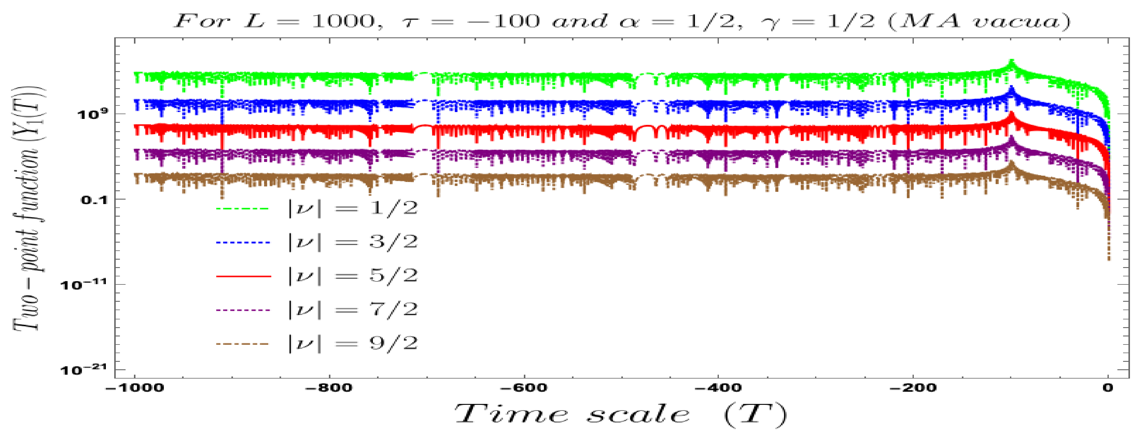
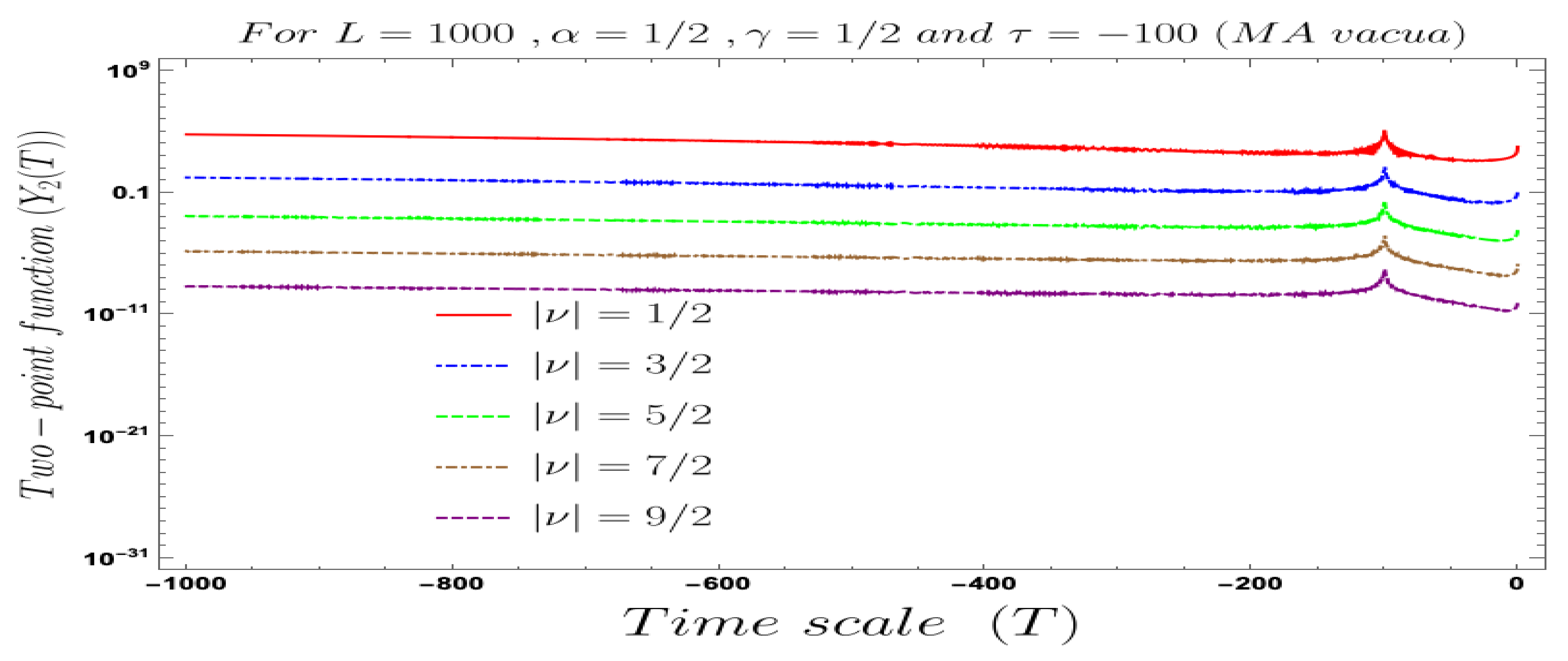
• In Figure 6 and Figure 7, conformal time dependent behaviour of the two-point auto-correlated field and momentum OTO functions with respect to the two time scales is explicitly shown. From these plots, it is clearly observed that with respect to both the time scales the two-point auto-correlated field and momentum OTO functions show random fluctuating behaviour.
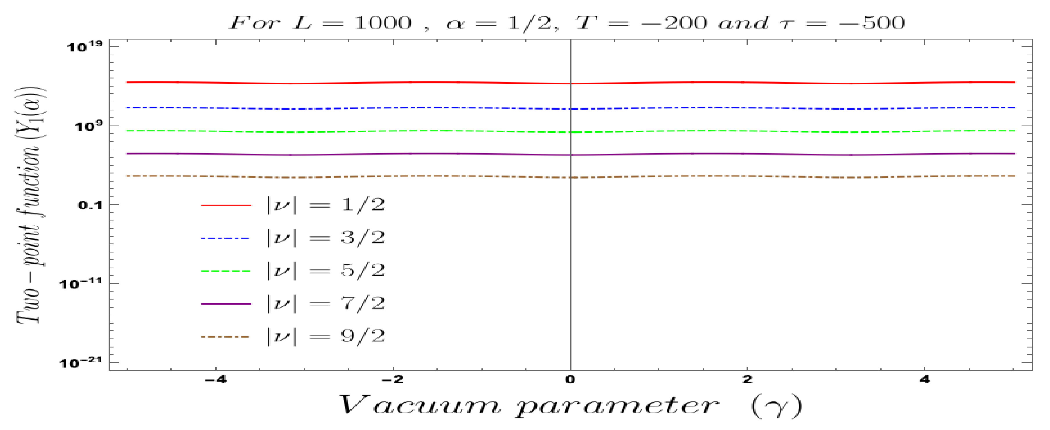
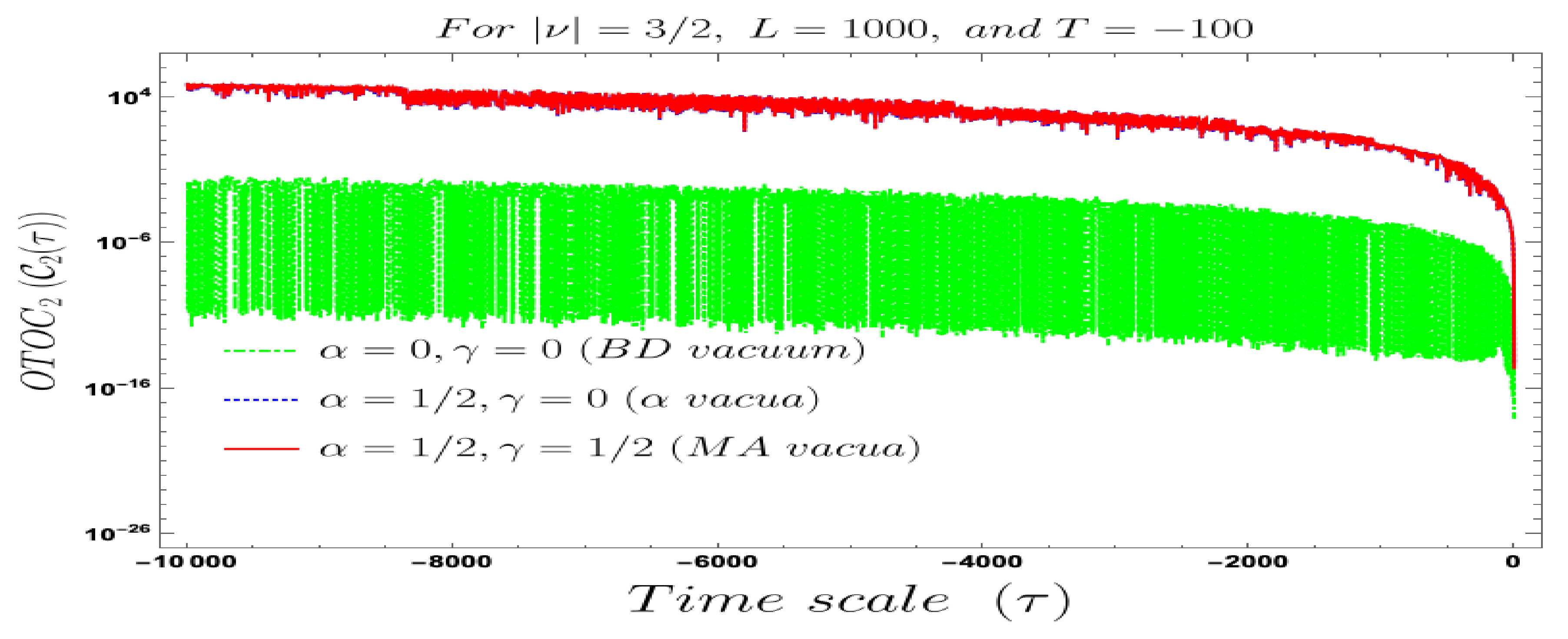
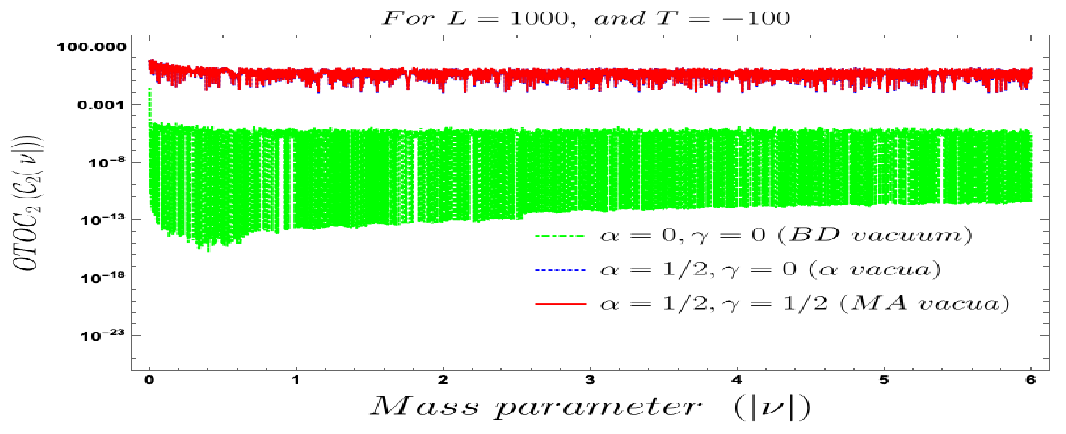
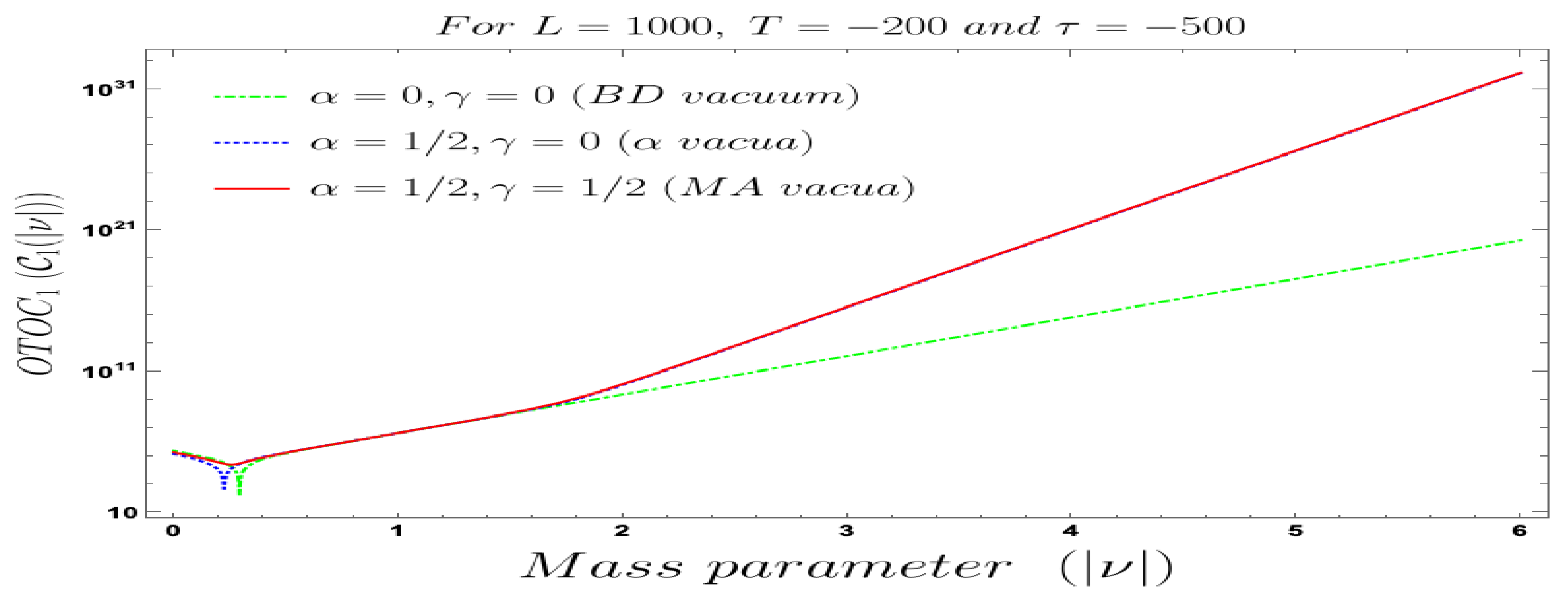
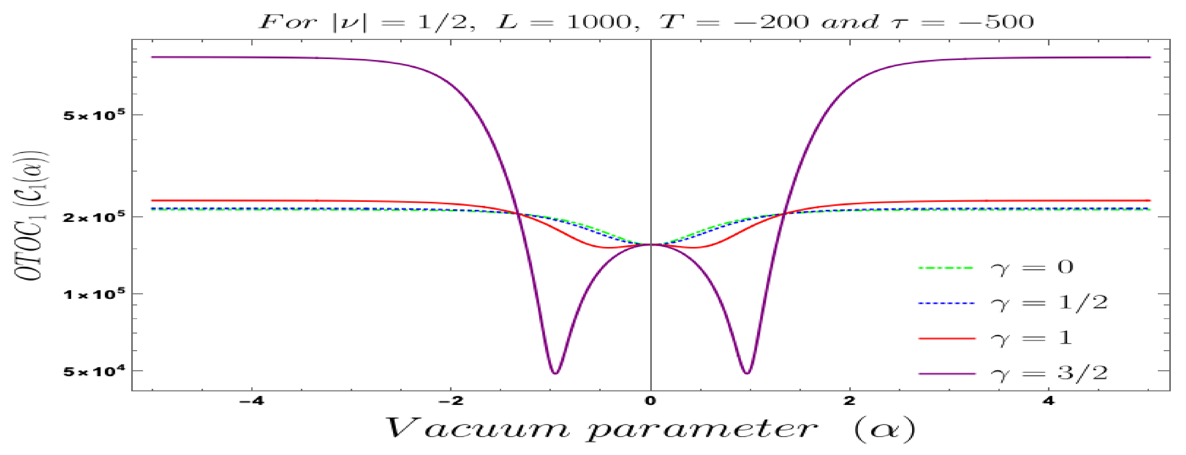
• For both the cases, it is observed that we get the significant distinguishable features in the time-dependent two-point auto-correlated field and momentum OTO functions for partially massless or heavy scalar fields. In Figure 8, if we change the quantum initial conditions by changing the vacuum state by introducing the non-standard Mota–Allen vacua, then a clear distinctive feature can be observed by changing the vacuum parameters $\alpha$ and $\gamma$, respectively. The behaviour of the two-point auto-correlated field and momentum OTO functions is explicitly depicted in Figure 9 and Figure 10. From these plots, one can clearly see that for the results obtained using Bunch–Davies vacuum, $\alpha$ vacua and Mota–Allen vacua state initial conditions, the two-point auto-correlated field and momentum OTO functions significantly decay very fast in a non-standard fashion with respect to the magnitude of the mass parameter $\left|\nu \right|$ for partially massless and heavy scalar fields in primordial cosmology. We have explicitly shown the behaviour of the two-point auto-correlated field and momentum OTO functions for $\alpha =1/2,\gamma =1/2$, where it is clearly observed that the correlation decays very rapidly with the increase in the magnitude of the mass parameter $\left|\nu \right|$.
• In addition, we have observed from the plots that the random fluctuations with respect to the conformal time scale show decaying time-dependent behaviour at the very late time scale. First of all, all of them show a saturating behaviour and then it increases at a particular value in the time scale and then these plots show decaying features. This large peak value of the two-point auto-correlated spectra is obtained at the scale when the two time scales of the theory becomes comparable. Physically, this is a very crucial fact as it shows at this particular time scale we are actually getting zero information from the two-point auto-correlations. Only the preferred information can be extracted from the very early time scale as well as at the very late time scale after the peak.

5. Numerical Analysis II: Interpretation of Four-Point Non-Chaotic Auto-Correlated OTO Functions

Now comparing the results of the four-point auto-correlated field and momentum OTO functions, we get the following outcomes which are mentioned point-wise:

• Before normalising the four-point auto-correlated field and momentum OTO functions, the results computed from rescaled field and momentum and the curvature perturbation field variable and its conjugate momenta, the sides are not at all the same and are connected via a time-dependent Mukhanov–Sasaki variable dependent conformal factor ${\left(z\left({\tau }_1\right)z\left({\tau }_2\right)\right)}^{-2}$ in the final results.
• After normalising the four-point auto-correlated field and momentum OTO functions, the results computed from rescaled field and momentum and the curvature perturbation field variable and its conjugate momenta, the sides are not at all the same. In this case, particularly for the computational purpose, it is the best one as we really do not care about the origin of the quantum operators in the cosmological perturbation theory.

Next, we give the interpretation of the obtained results for the normalised four-point auto-correlated field and momentum OTO functions computed in the present setup point-wise:

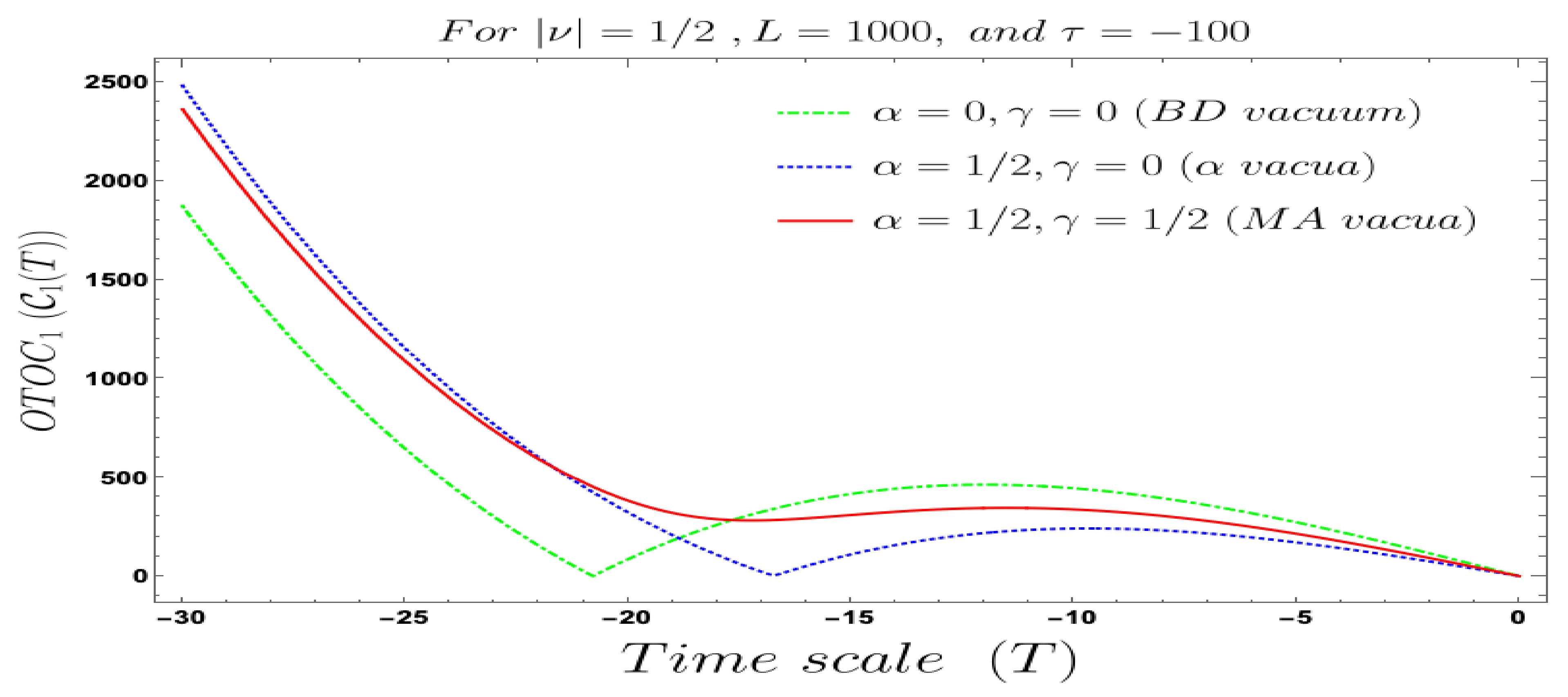
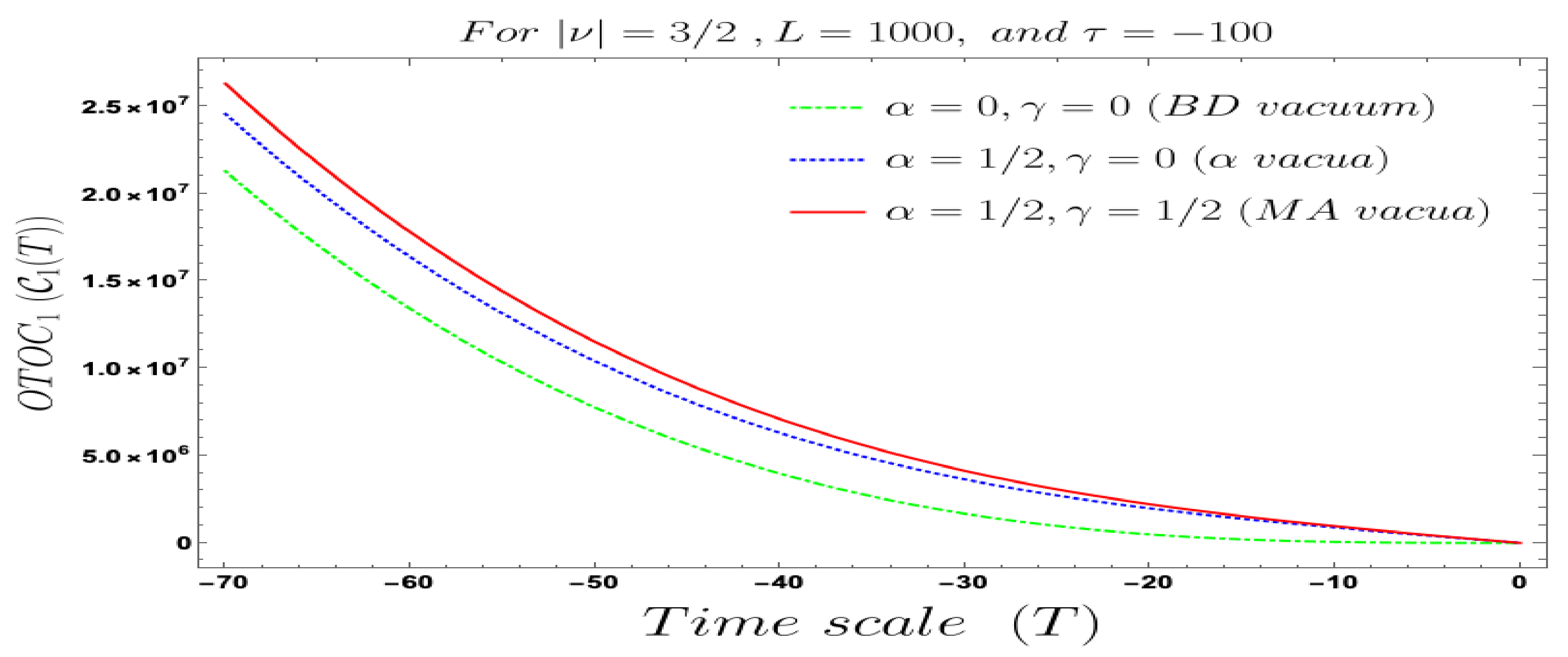
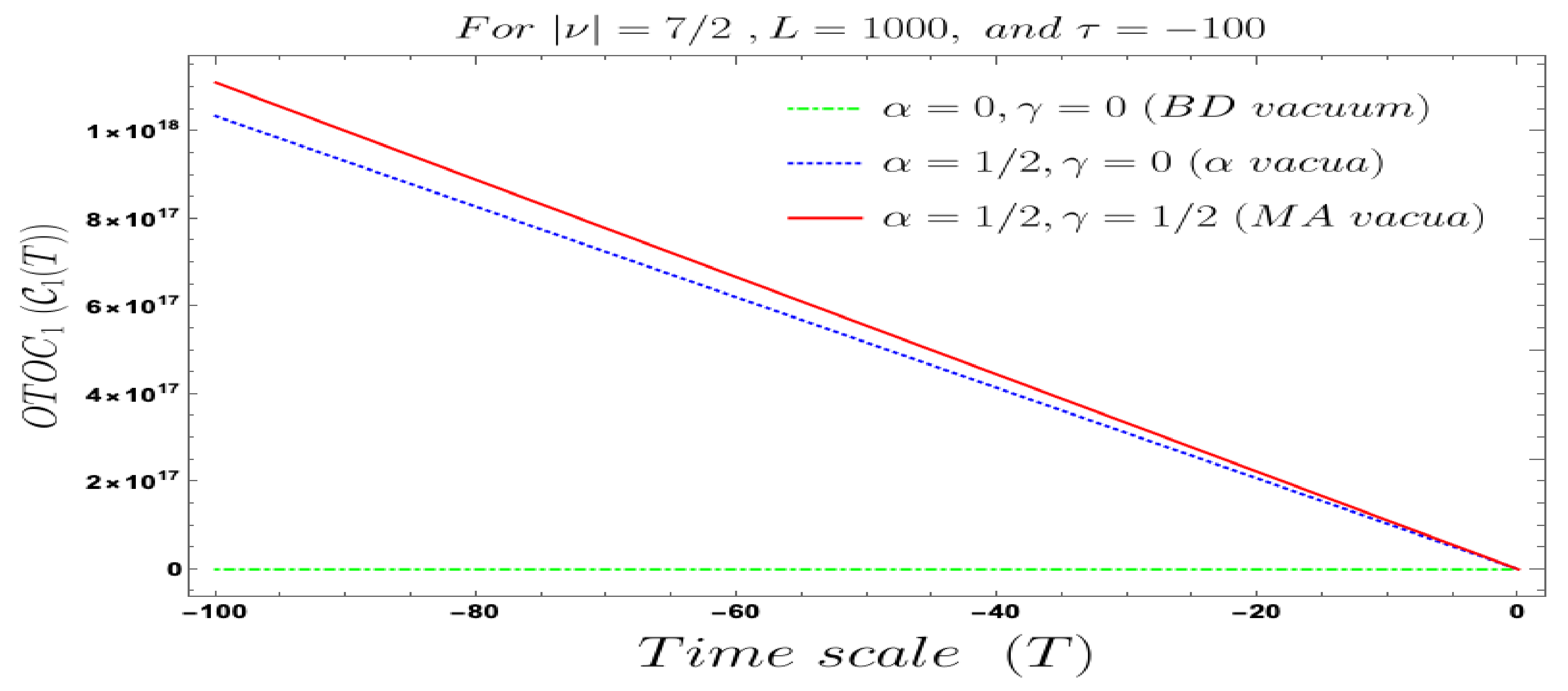
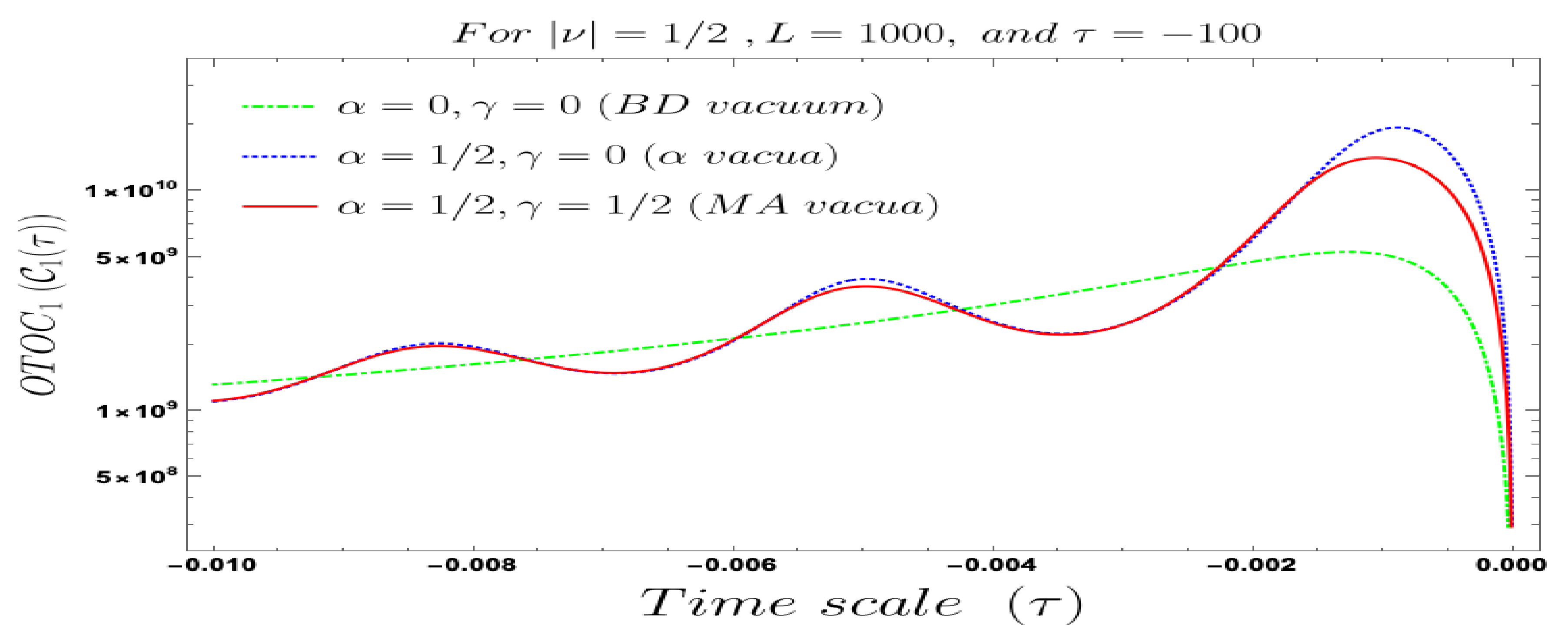
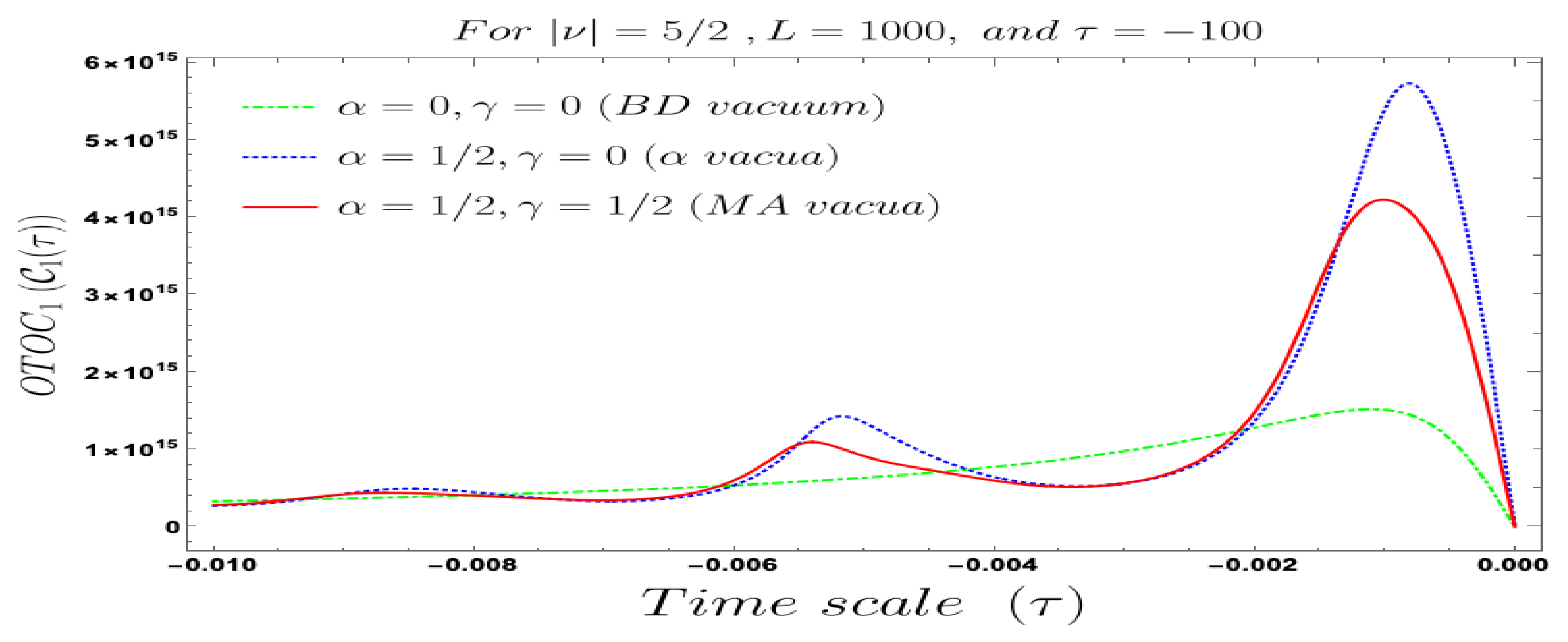
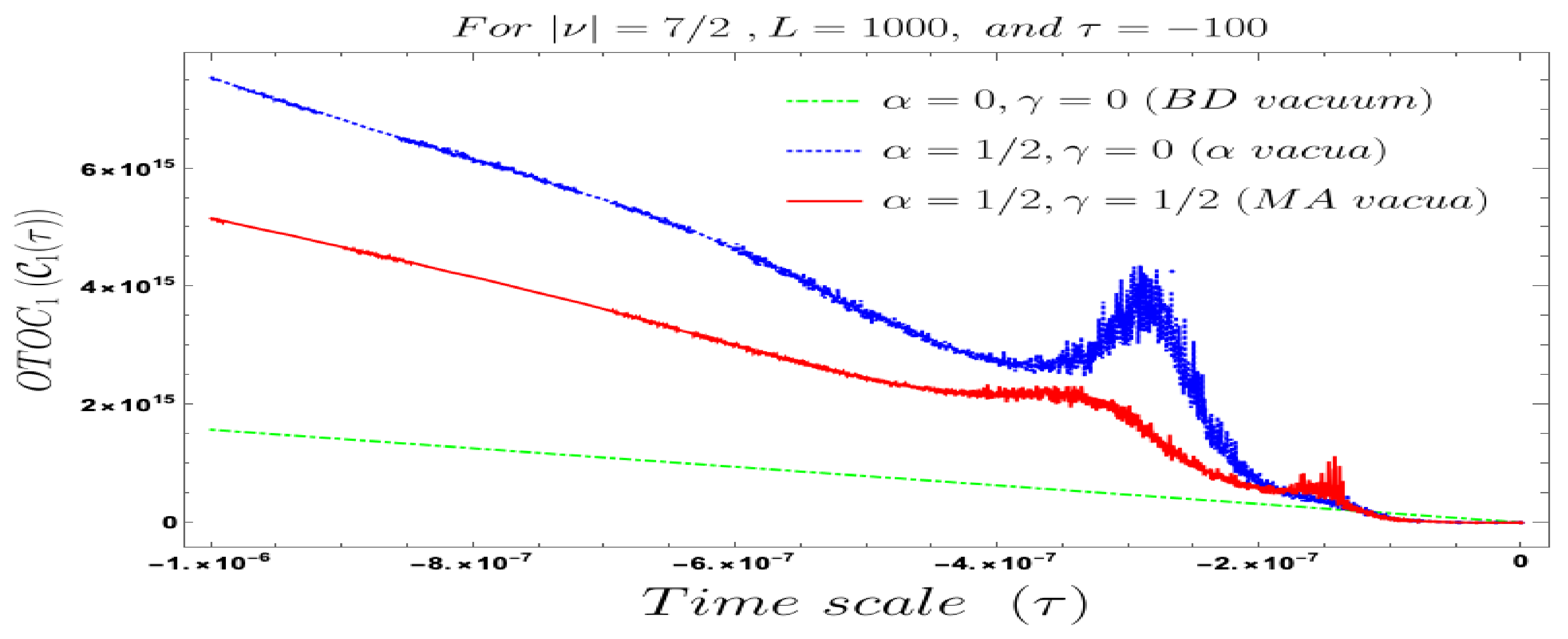
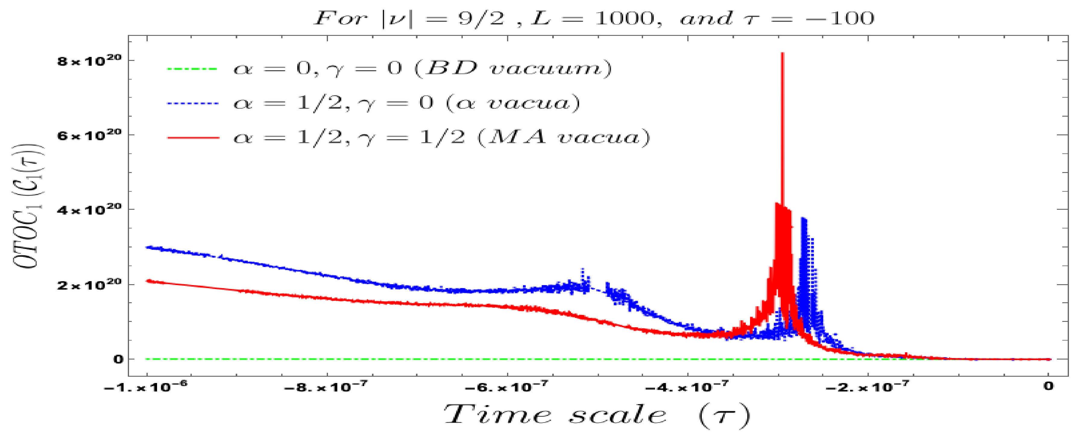
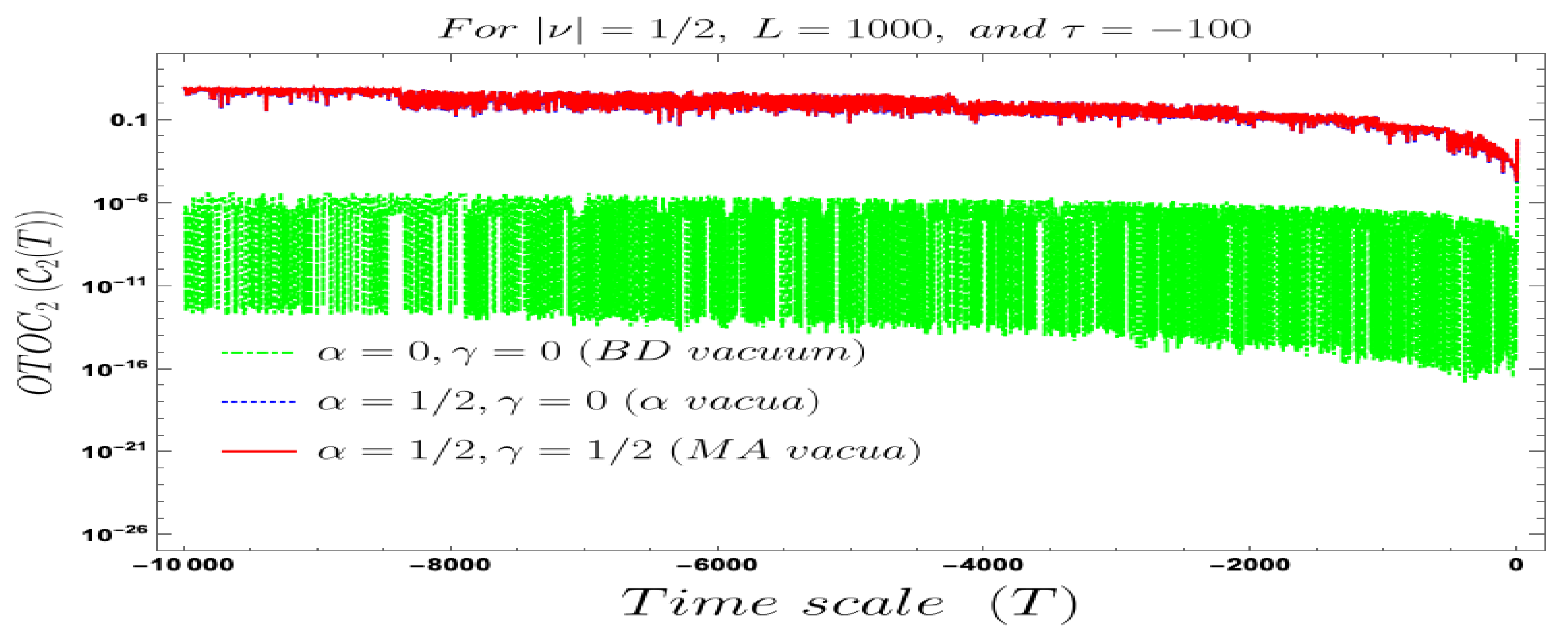
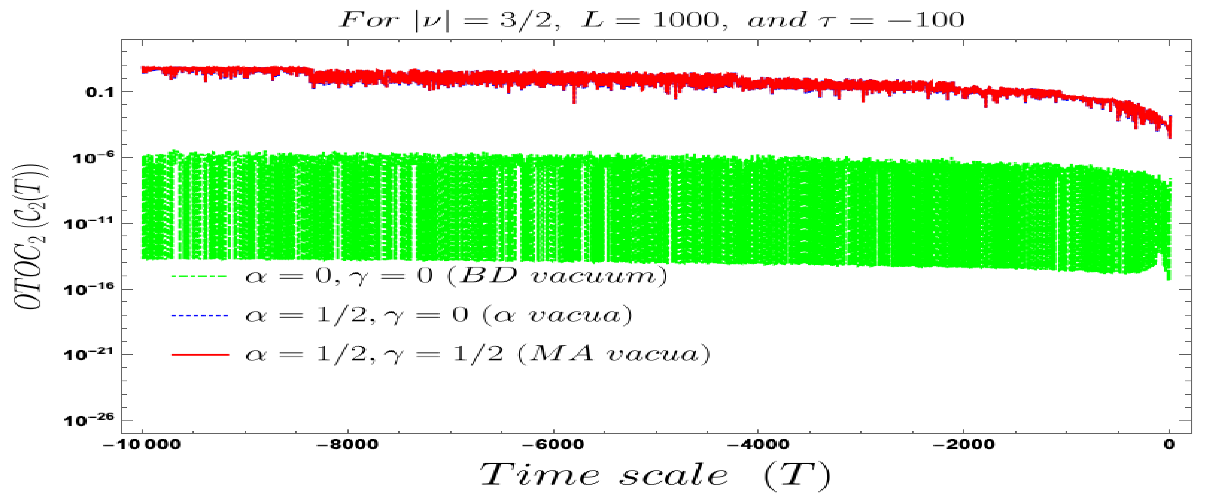
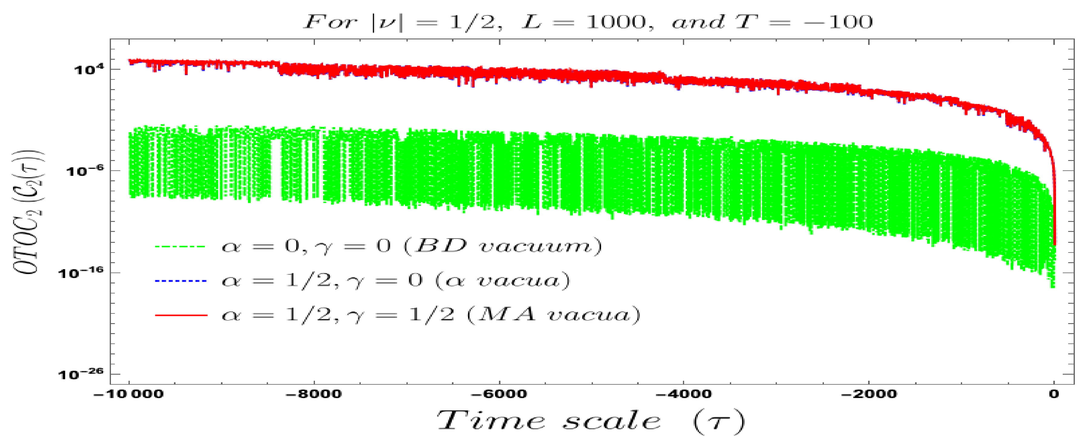
• In our computed four-point auto-correlated field and momentum OTO functions, two time scales are involved. During the study of the behaviour of the four-point auto-correlated field and momentum OTO functions, we have actually fixed one time scale and have studied the time-dependent dynamical behaviour with respect to the other time scale. We have found the behaviour with respect to both ${\tau }_1=T$ and ${\tau }_2=\tau$, using Bunch–Davies, $\alpha$ and the generalised Mota–Allen vacua as the initial choice of quantum vacuum state. See Figure 11, Figure 12, Figure 13, Figure 14, Figure 15, Figure 16, Figure 17, Figure 18, Figure 19, Figure 20, Figure 21 and Figure 22 for more information about the detailed conformal time-dependent feature of the normalised four-point auto-correlated field and momentum OTO functions. In the conformal time scale, all of these plots vary from $-\infty$ (Big Bang) to 0 (present day universe), and show significant distinctive features in the time scale.
• If we fix the time scale, ${\tau }_2=\tau$, and study the behaviour of the four-point auto-correlated field and momentum OTO functions with respect to the scale ${\tau }_1=T$, then we find that as we approach from the very early universe to the late time scale the normalised correlators show random non-standard non-chaotic behaviour.
• Additionally, we have found that we can get the desired features from the obtained results which can be visible only when the mass parameter, $\nu$, can be analytically continued to $-i\nu$. Therefore, massless De Sitter possibility ($\nu =3/2$) is not allowed. Consequently, we have the following options:
  • Partially massless De Sitter case is one of the possibilities where we can estimate the following parameter from the present understanding:

    $$\begin{array}{c}\hfill -i\nu =\sqrt{\frac{9}{4}-c^2}\mathrm{where}c\ge \sqrt{2},\end{array}$$

    (329)

    which implies the following bound on the mass parameter:

    $$\begin{array}{c}\hfill \nu \ge \frac{i}{2}.\end{array}$$

    (330)
    This is consistent with the plots obtained for the following values of the mass parameter:

    $$\begin{array}{c}\hfill \nu =\frac{i}{2},\frac{3i}{2},\frac{5i}{2},\frac{7i}{2},\frac{9i}{2}.\end{array}$$

    (331)
  • Massive De Sitter case is one of the possibilities where we can estimate the following parameter:

    $$\begin{array}{c}\hfill \nu =i\sqrt{\frac{m^2}{H^2}-\frac{9}{4}}.\end{array}$$

    (332)
    Since we have studied the case for $\nu \ge i/2$, we get the following bound on the mass of the heavy field:

    $$\begin{array}{c}\hfill m\ge \sqrt{\frac{5}{2}}H.\end{array}$$

    (333)
  • Reheating case is the last possibility, where we can estimate:

    $$\begin{array}{c}\hfill \frac{i}{2}\le \nu \le \frac{3i}{2}\mathrm{for}0\le w_{reh}\le \frac{1}{3}.\end{array}$$

    (334)
• After fixing both the time scales at far past, the behaviour of the four-point auto-correlated field and momentum OTO functions, with respect to the mass parameter, is depicted in the Figure 22 and Figure 23 for Bunch–Davies, $\alpha$ and Mota–Allen vacua as the quantum mechanical vacuum states.
• After fixing both the time scales at far past and fixing $\nu =i/2$, the behaviour of four-point auto-correlated field and momentum OTO functions with respect to the vacuum parameters $\alpha$ and $\gamma$ is depicted in Figure 24, Figure 25, Figure 26 and Figure 27.
• All the momentum-dependent integrals are divergent at ∞, for which we have introduced a UV regulator at $L=1000$ (large value). This makes the final results of four-point auto-correlated field and momentum OTO functions numerically convergent.
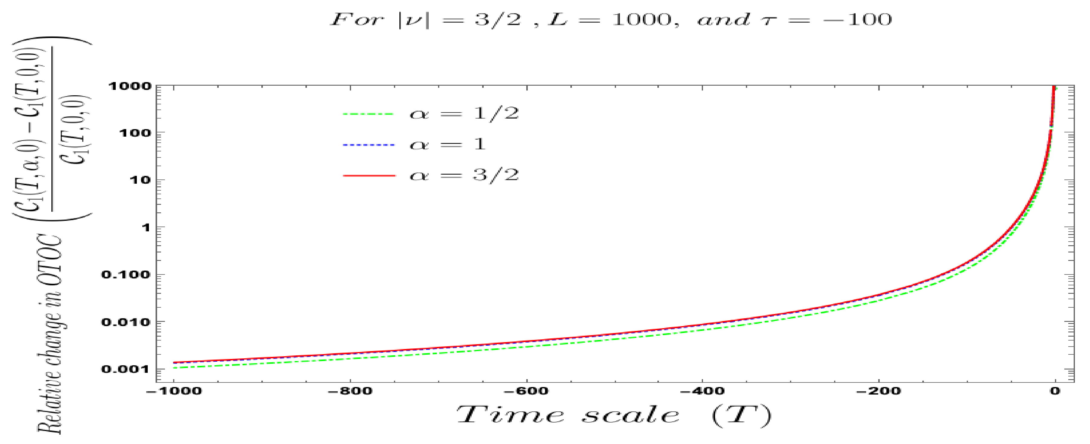
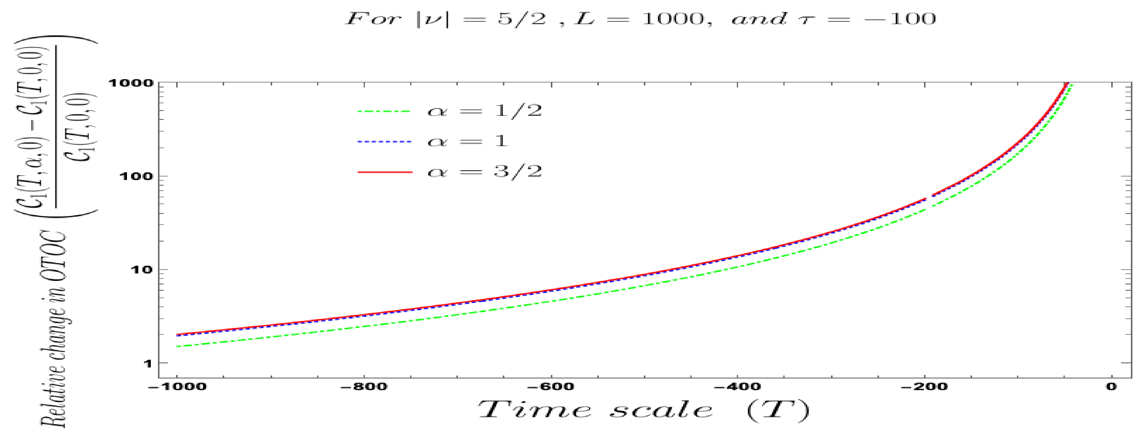
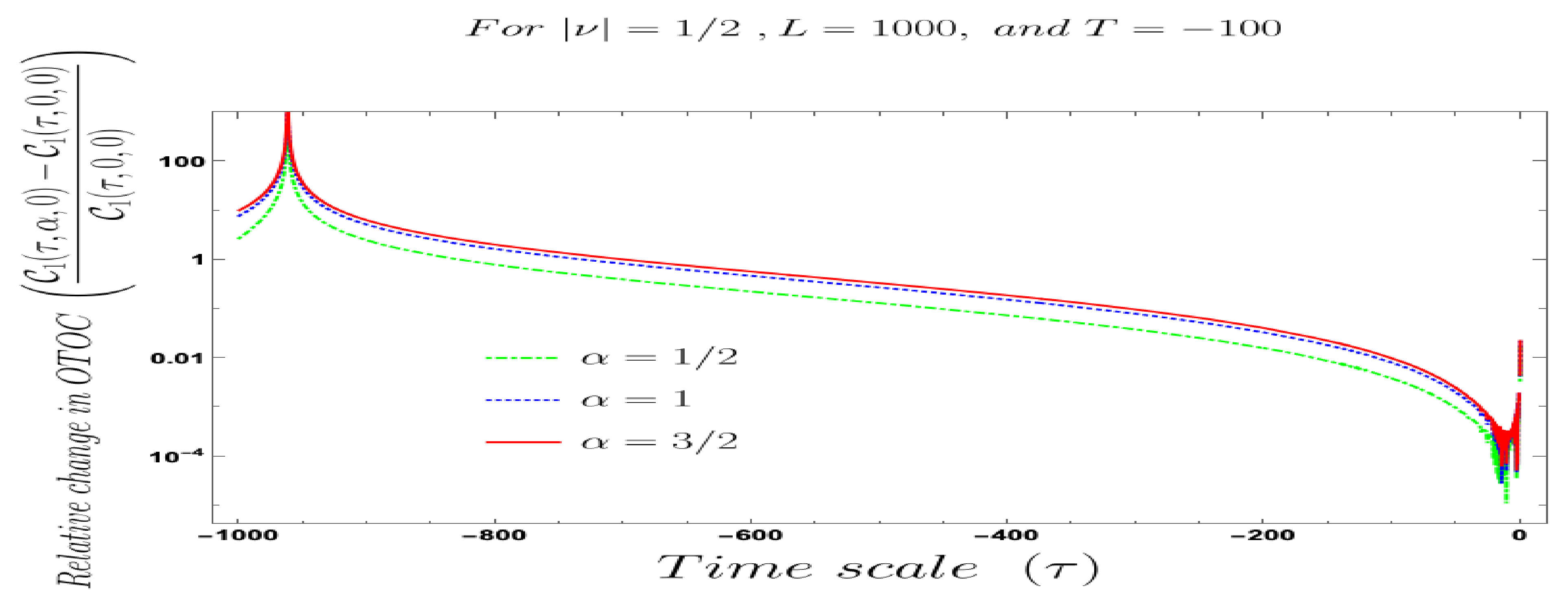
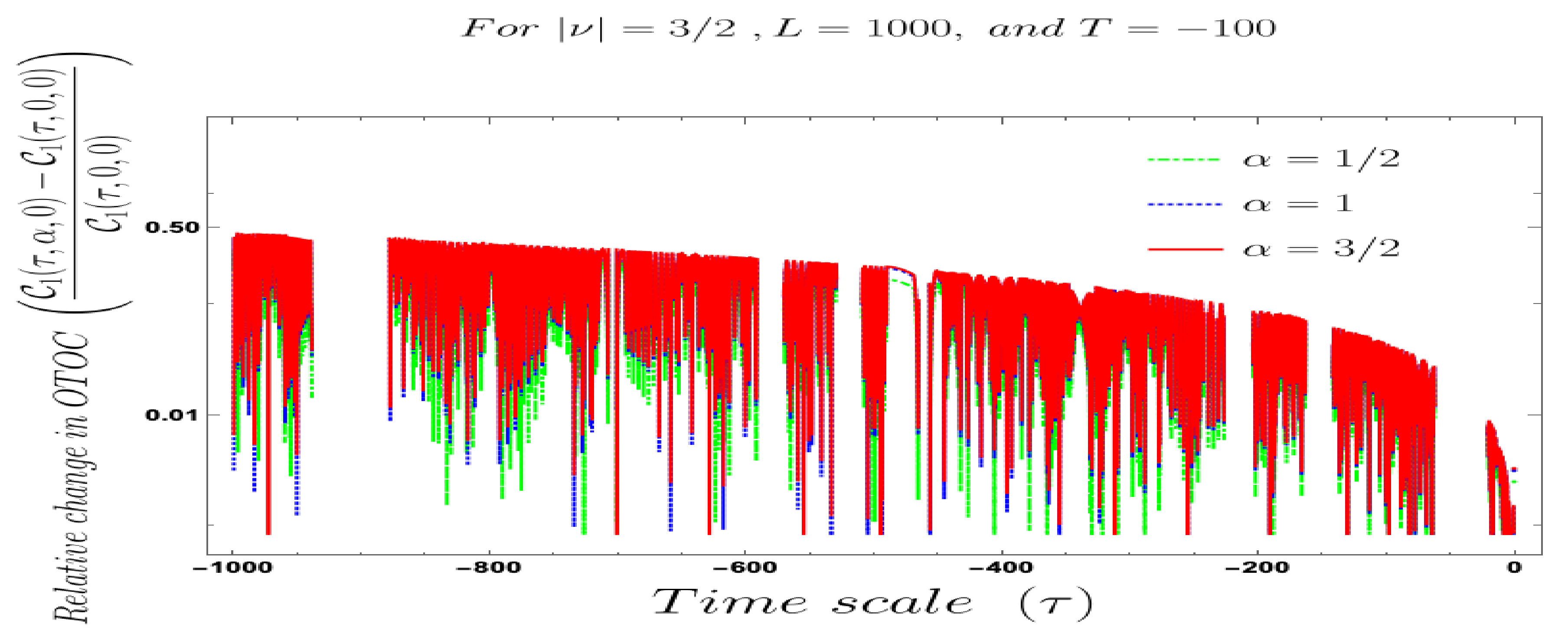
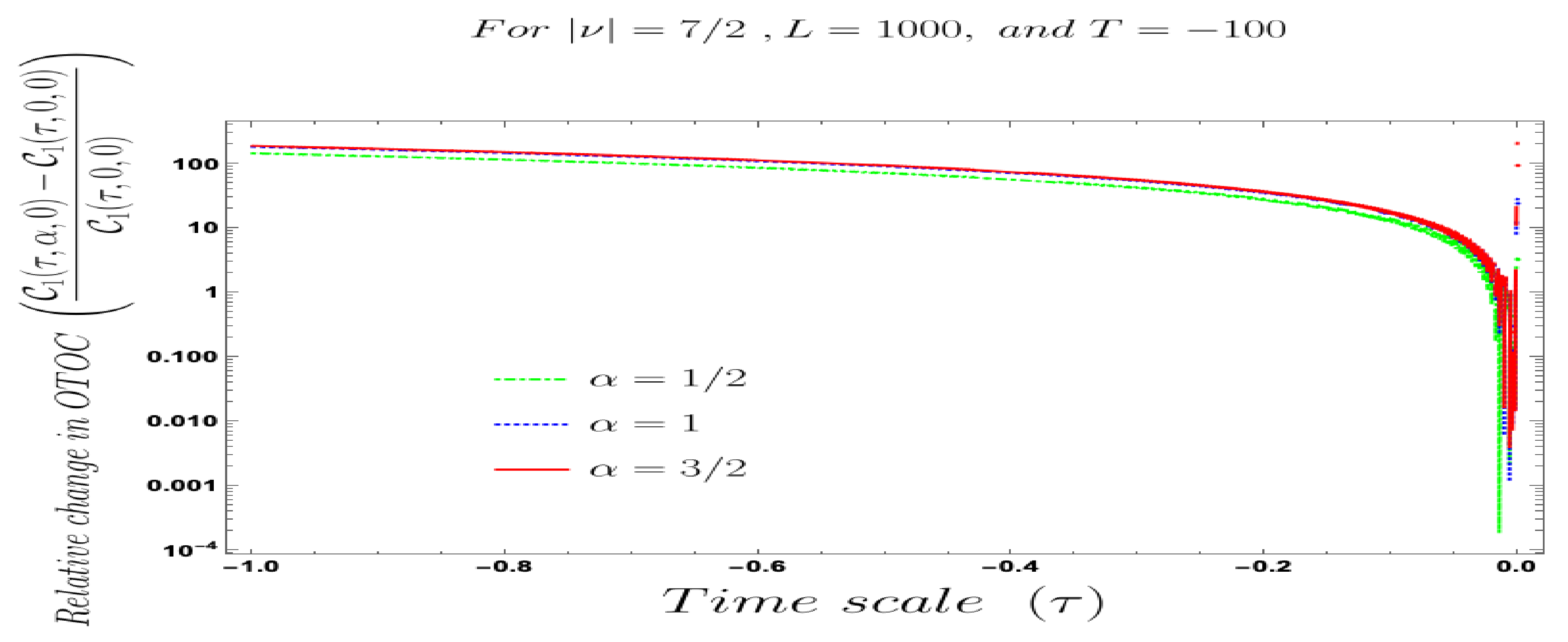
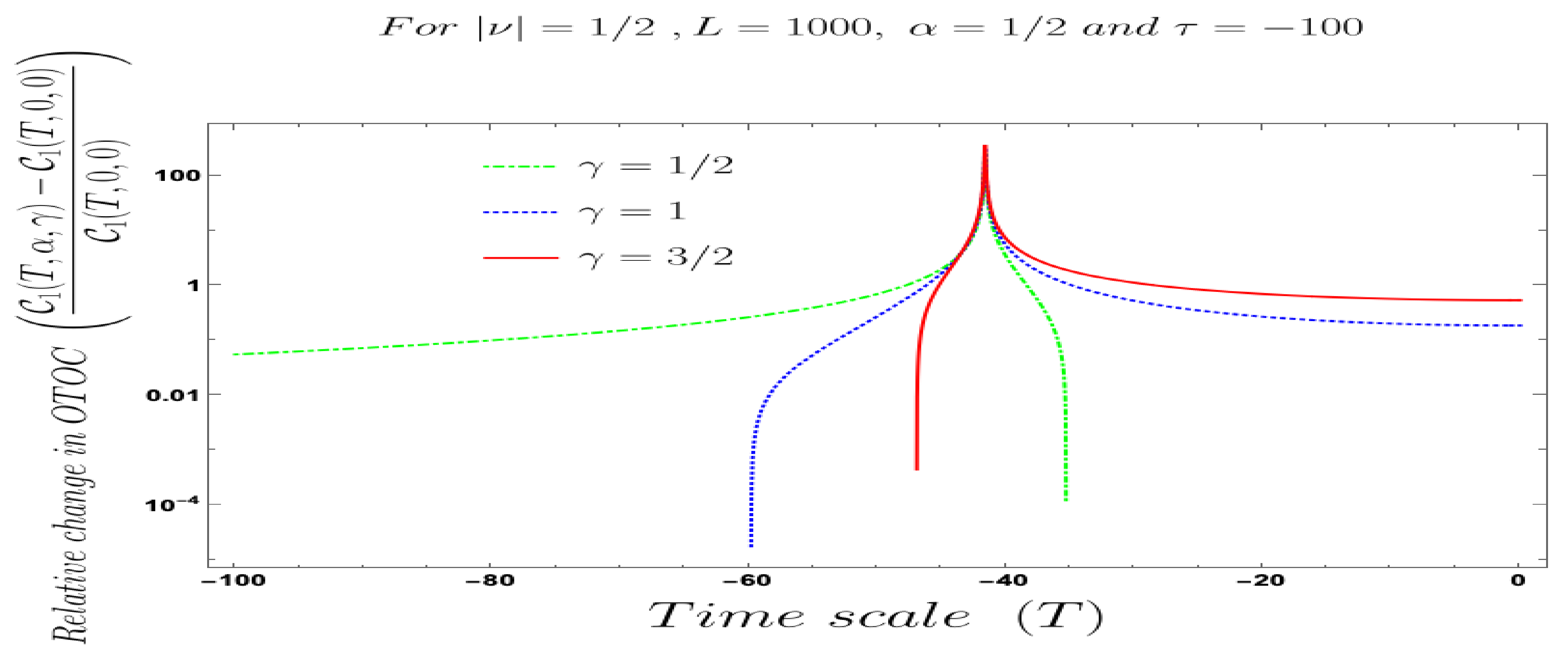
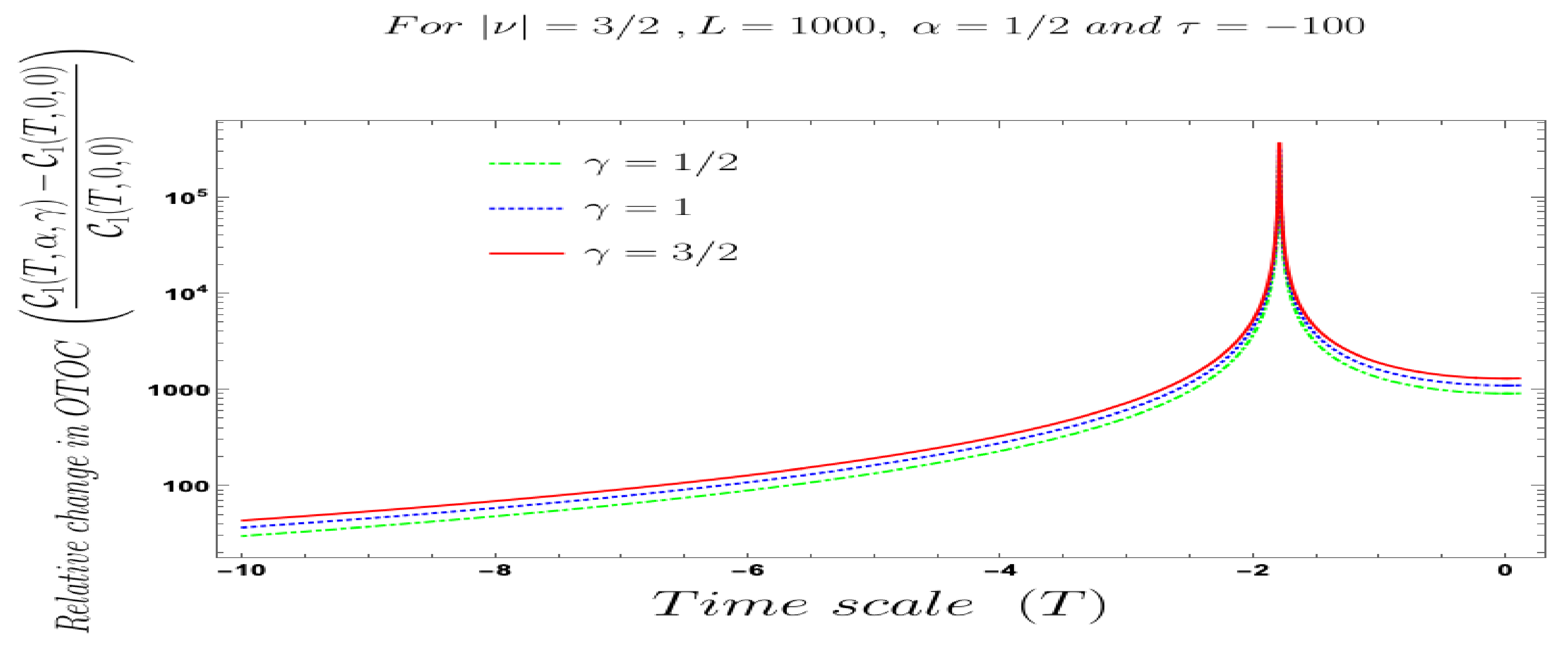
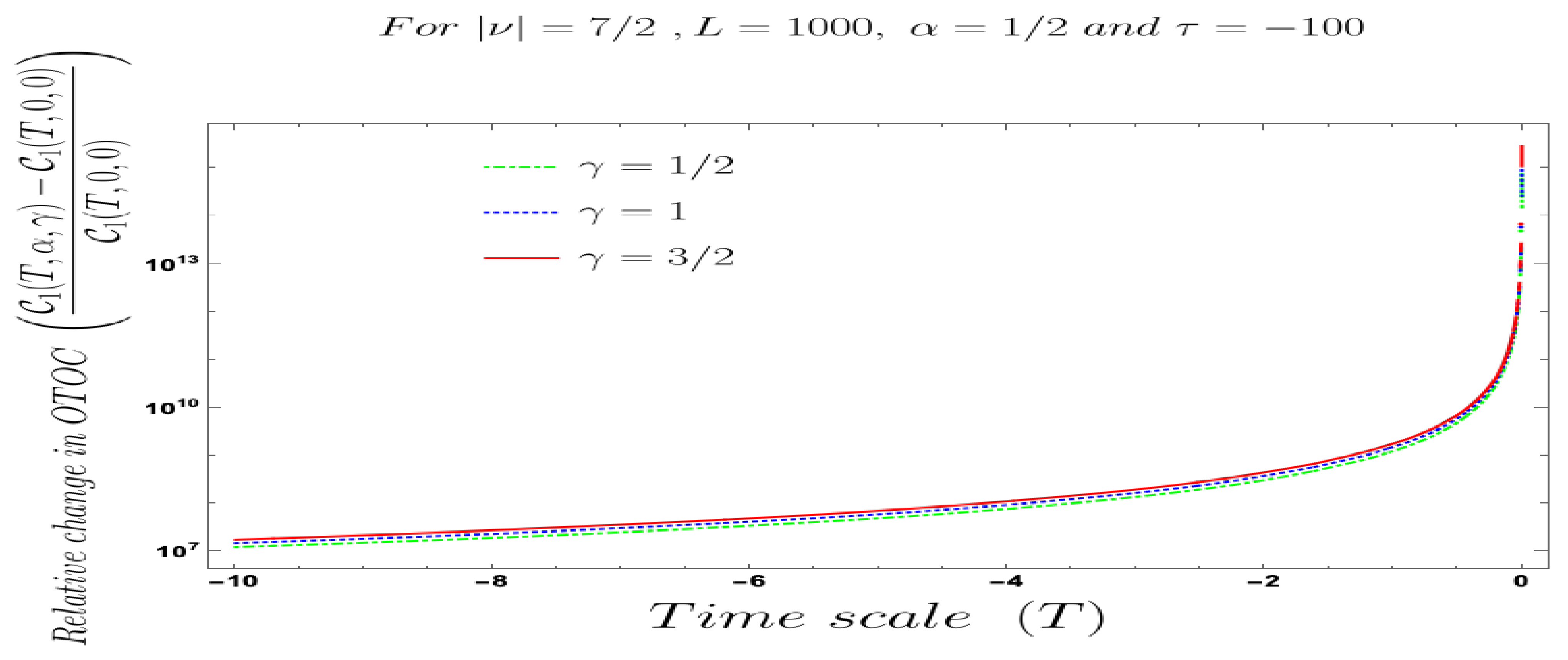
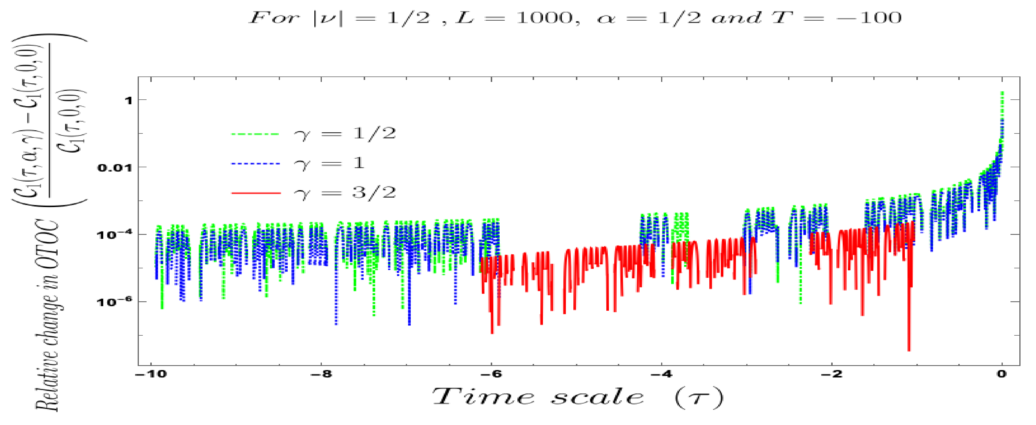
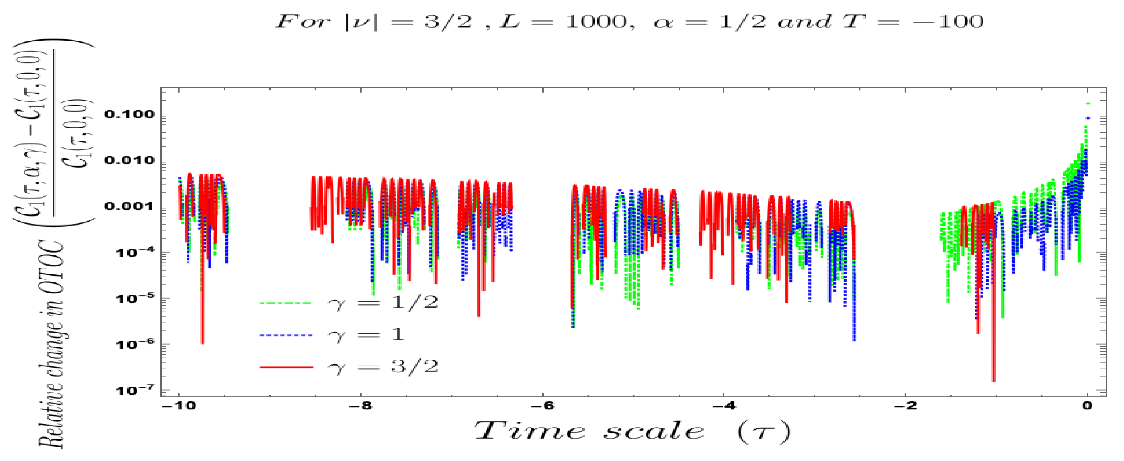
• Further, we define a relative change in normalised four-point auto-correlated field and momentum OTO functions where the relativeness is defined with respect to the definition of quantum mechanical vacuum state, given by:

  $$\begin{array}{ccc}& & {\mathcal{R}}_{\alpha ,\gamma }^{\left(p\right)}\left({\tau }_i\right)=\left(\frac{\underset{\mathbf{Motta}--\mathbf{Allen}\mathbf{vacua}}{\underbrace{{\mathcal{C}}_p({\tau }_i,\alpha ,\gamma )}}-\underset{\mathbf{Bunch}--\mathbf{Davies}\mathbf{vacuum}}{\underbrace{{\mathcal{C}}_p({\tau }_i,\alpha =0,\gamma =0)}}}{\underset{\mathbf{Bunch}--\mathbf{Davies}\mathbf{vacuum}}{\underbrace{{\mathcal{C}}_p({\tau }_i,\alpha =0,\gamma =0)}}}\right)\forall i=1\left(T\right),2\left(\tau \right)\hfill \\ & & \&\forall p=1\left(\mathrm{Field}\mathrm{auto}\mathrm{correlator}\right),2\left(\mathrm{Momentum}\mathrm{auto}\mathrm{correlator}\right).\hfill \end{array}$$

  (335)
  In Figure 28, Figure 29, Figure 30, Figure 31, Figure 32, Figure 33, Figure 34, Figure 35, Figure 36, Figure 37 and Figure 38, we have explicitly shown the behaviour of the relative change in normalised four-point auto-correlated field and momentum OTO functions with respect to the two time scales. Here is the relative change we have studied for $\alpha =1/2,\gamma =1^{\prime }2$, $\alpha =1/2,\gamma =1$ and $\alpha =1/2,\gamma =3/2$ with respect to $\alpha =0$ for all previously allowed values of the mass parameters for partially massless and heavy scalar fields. From this relative change, one can also study the large or small deviation from the Bunch–Davies result compared to the other results obtained from all non-standard quantum vacuum states.
• In addition, we have to mention here that the computed four-point auto-correlated field and momentum OTO functions are independent of any specific choice of the coordinate system. Finally, we get a momentum integrated cut-off regulated result for the four-point auto-correlated field and momentum OTO functions which only depend on the two dynamical conformal time scales on which we have defined the rescaled perturbation variable and its canonically conjugate momenta. This is quite a good outcome. In the generalised prescriptions, when one introduces the quantum operators in a specific time and coordinate system, it always appears that in the final result it captures the effect of inhomogeneity in the space-time coordinate. In the context of spatially flat FLRW cosmology, we have found that the final result of the four-point auto-correlated field and momentum OTO functions captures the effect of inhomogeneity. This is because in cosmology we are actually interested in the time evolution of the quantum operators which are separated in time scale, which is one of the crucial constraints in the definition of any general four-point auto-correlated field and momentum OTO function. Such four-point auto-correlated field and momentum OTO functions do not capture the inhomogeneity.
• The final result of the four-point auto-correlated field and momentum OTO functions are not explicitly dependent on the factor $\beta =1/T$ which is appearing in the expression for the thermal partition function. This further implies that the final results are also independent of the thermal partition function computed for primordial cosmology.

6. Classical Limit of Non-Chaotic Auto-Correlated OTO Amplitudes and OTOC in Primordial Cosmology

6.1. Computational Strategy for Non-Chaotic Auto-Correlated OTO Functions in the Classical Limit

In this section, our prime objective is to study the classical limit of the four-point auto-correlation functions that we have explicitly derived from the quantum descriptions. In the following subsections, we will derive the classical limiting results which will be consistent with the super-horizon late time limiting behaviour of the cosmological auto-correlated functions.

In this subsection, we will illustrate our computational strategy to study the classical limit of the cosmological four-point OTOC derived in this paper:

• First of all, we have to take the quantum to classical map. For this purpose, we consider the classical mode function and its canonically conjugate momentum which we have derived in an earlier section of this paper.
• Next, in the classical limit, we use the Poisson brackets of the classical mode function and its canonically conjugate momentum variables in cosmological perturbation theory.
• In the classical limit, the definition of quantum trace will be replaced by phase-space volume measure, ${\displaystyle \frac{{\displaystyle d{f}_{\mathbf{k}}\left(\tau \right)d{\mathsf{\Pi }}_{\mathbf{k}}\left(\tau \right)}}{{\displaystyle 2\pi }}}$, which mimics the role of path integral measure, ${\displaystyle \frac{\mathcal{D}{f}_{\mathbf{k}}\left(\tau \right)\mathcal{D}{\mathsf{\Pi }}_{\mathbf{k}}\left(\tau \right)}{2\pi }}$, in the classical limit.
• In addition, during this computation, we have to include an additional thermal Boltzmann factor which is serving the purpose of thermal weight factor taking the phase-space average over the classical micro-canonical statistical ensemble.
• Next, we compute the expression for the classical thermal partition function for cosmological perturbations which is consistent with the quantum result computed from completely different formalism. To compute the classical partition function one need to compute the expression by following the principles of classical statistical mechanics very carefully. We will show that the final expressions for the classical limit of auto-correlated OTOs are independent of the partition function for the cosmological scenario in which we are interested in.
• Last but not least, we compute the expression for the normalisation factor for the classical limiting version of the auto-correlated OTO functions by following the above-mentioned general formalism.

6.2. Classical Limit of Cosmological Two-Point “In-In” Non-Chaotic OTO Amplitudes

To compute the classical limit, we start with the Poisson bracket of these cosmologically relevant canonically conjugate operators, which are given by the following expressions:

$$\begin{array}{ccc}\hfill {\left\{f(\mathbf{x},{\tau }_1),f(\mathbf{x},{\tau }_2)\right\}}_{\mathbf{PB}}& =& \int \frac{d^3{\mathbf{k}}_1}{{\left(2\pi \right)}^3}\int \frac{d^3{\mathbf{k}}_2}{{\left(2\pi \right)}^3}exp(i({\mathbf{k}}_1+{\mathbf{k}}_2).\mathbf{x})\hfill \\ & & \left[{\left\{f_{{\mathbf{k}}_1}\left({\tau }_1\right),f_{{\mathbf{k}}_2}\left({\tau }_2\right)\right\}}_{\mathbf{PB}}+{\left\{f_{{\mathbf{k}}_2}\left({\tau }_1\right),f_{{\mathbf{k}}_1}\left({\tau }_2\right)\right\}}_{\mathbf{PB}}\right],\hfill \end{array}$$

(336)

$$\begin{array}{ccc}\hfill {\left\{\mathsf{\Pi }(\mathbf{x},{\tau }_1),\mathsf{\Pi }(\mathbf{x},{\tau }_2)\right\}}_{\mathbf{PB}}& =& \int \frac{d^3{\mathbf{k}}_1}{{\left(2\pi \right)}^3}\int \frac{d^3{\mathbf{k}}_2}{{\left(2\pi \right)}^3}exp(i({\mathbf{k}}_1+{\mathbf{k}}_2).\mathbf{x})\hfill \\ & & \left[{\left\{{\mathsf{\Pi }}_{{\mathbf{k}}_1}\left({\tau }_1\right),{\mathsf{\Pi }}_{{\mathbf{k}}_2}\left({\tau }_2\right)\right\}}_{\mathbf{PB}}+{\left\{{\mathsf{\Pi }}_{{\mathbf{k}}_2}\left({\tau }_1\right),{\mathsf{\Pi }}_{{\mathbf{k}}_1}\left({\tau }_2\right)\right\}}_{\mathbf{PB}}\right].\hfill \end{array}$$

(337)

In the Fourier transformed space, the individual Poisson brackets are given by the following expressions:

$$\begin{array}{ccc}\hfill {\left\{f_{{\mathbf{k}}_1}\left({\tau }_1\right),f_{{\mathbf{k}}_2}\left({\tau }_2\right)\right\}}_{\mathbf{PB}}& =& {\left(2\pi \right)}^3{\delta }^3({\mathbf{k}}_1+{\mathbf{k}}_2){\mathbf{R}}_1({\tau }_1,{\tau }_2),\hfill \end{array}$$

(338)

$$\begin{array}{ccc}\hfill {\left\{f_{{\mathbf{k}}_2}\left({\tau }_1\right),f_{{\mathbf{k}}_1}\left({\tau }_2\right)\right\}}_{\mathbf{PB}}& =& {\left(2\pi \right)}^3{\delta }^3({\mathbf{k}}_2+{\mathbf{k}}_1){\mathbf{R}}_1({\tau }_1,{\tau }_2),\hfill \end{array}$$

(339)

$$\begin{array}{ccc}\hfill {\left\{{\mathsf{\Pi }}_{{\mathbf{k}}_1}\left({\tau }_1\right),{\mathsf{\Pi }}_{{\mathbf{k}}_2}\left({\tau }_2\right)\right\}}_{\mathbf{PB}}& =& {\left(2\pi \right)}^3{\delta }^3({\mathbf{k}}_1+{\mathbf{k}}_2){\mathbf{R}}_2({\tau }_1,{\tau }_2),\hfill \end{array}$$

(340)

$$\begin{array}{ccc}\hfill {\left\{{\mathsf{\Pi }}_{{\mathbf{k}}_2}\left({\tau }_1\right),{\mathsf{\Pi }}_{{\mathbf{k}}_1}\left({\tau }_2\right)\right\}}_{\mathbf{PB}}& =& {\left(2\pi \right)}^3{\delta }^3({\mathbf{k}}_2+{\mathbf{k}}_1){\mathbf{R}}_2({\tau }_1,{\tau }_2),\hfill \end{array}$$

(341)

which further implies the following symmetric result:

$$\begin{array}{ccc}\hfill {\left\{f_{{\mathbf{k}}_1}\left({\tau }_1\right),f_{{\mathbf{k}}_2}\left({\tau }_2\right)\right\}}_{\mathbf{PB}}& =& {\left\{f_{{\mathbf{k}}_2}\left({\tau }_1\right),f_{{\mathbf{k}}_1}\left({\tau }_2\right)\right\}}_{\mathbf{PB}}={\left(2\pi \right)}^3{\delta }^3({\mathbf{k}}_1+{\mathbf{k}}_2){\mathbf{R}}_1({\tau }_1,{\tau }_2),\hfill \end{array}$$

(342)

$$\begin{array}{ccc}\hfill {\left\{{\mathsf{\Pi }}_{{\mathbf{k}}_1}\left({\tau }_1\right),{\mathsf{\Pi }}_{{\mathbf{k}}_2}\left({\tau }_2\right)\right\}}_{\mathbf{PB}}& =& {\left\{{\mathsf{\Pi }}_{{\mathbf{k}}_2}\left({\tau }_1\right),{\mathsf{\Pi }}_{{\mathbf{k}}_1}\left({\tau }_2\right)\right\}}_{\mathbf{PB}}={\left(2\pi \right)}^3{\delta }^3({\mathbf{k}}_1+{\mathbf{k}}_2){\mathbf{R}}_2({\tau }_1,{\tau }_2),\hfill \end{array}$$

(343)

which is appearing due to the fact that the three dimensional Dirac Delta function is symmetric under the exchange of two different momenta.

Now we define the two-point random classical correlation functions ${\mathbf{R}}_1({\tau }_1,{\tau }_2)$ and ${\mathbf{R}}_2({\tau }_1,{\tau }_2)$ by the following expressions:

$$\begin{array}{ccc}\hfill {\mathbf{R}}_1({\tau }_1,{\tau }_2):& =& {\mathbf{W}}_1({\tau }_1-{\tau }_2)\hfill \end{array}$$

(344)

$$\begin{array}{ccc}\hfill {\mathbf{R}}_2({\tau }_1,{\tau }_2):& =& {\mathbf{W}}_2({\tau }_1-{\tau }_2),\hfill \end{array}$$

(345)

where ${\mathbf{W}}_1({\tau }_1-{\tau }_2)$ and ${\mathbf{W}}_2({\tau }_1-{\tau }_2)$ are the two window functions which are defined as:

$$\begin{array}{ccc}\hfill {\mathbf{W}}_1({\tau }_1-{\tau }_2)& =& \sqrt{\langle {\eta }_{\mathbf{Noise}}\left({\tau }_1\right){\eta }_{\mathbf{Noise}}\left({\tau }_2\right)\rangle },\hfill \end{array}$$

(346)

$$\begin{array}{ccc}\hfill {\mathbf{W}}_2({\tau }_1-{\tau }_2)& =& \sqrt{\langle {\mathsf{\Pi }}_{{\eta }_{\mathbf{Noise}}}\left({\tau }_1\right){\mathsf{\Pi }}_{{\eta }_{\mathbf{Noise}}}\left({\tau }_2\right)\rangle }.\hfill \end{array}$$

(347)

where the two-point noise and its associate canonically conjugate momentum correlation functions at the classical level are given by the following expressions:

$$\begin{array}{ccc}& & \langle {\eta }_{\mathbf{Noise}}\left({\tau }_1\right){\eta }_{\mathbf{Noise}}\left({\tau }_2\right)\rangle :=\sqrt{{\mathbf{G}}_{\mathbf{kernel}}^{\left(1\right)}({\tau }_1-{\tau }_2)}=\sqrt{{\mathbf{G}}_{\mathbf{kernel}}^{\left(1\right)}({\tau }_2-{\tau }_1)}\equiv \sqrt{{\mathbf{G}}_{\mathbf{kernel}}^{\left(1\right)}\left(\right|{\tau }_1-{\tau }_2\left|\right)},\hfill \end{array}$$

(348)

$$\begin{array}{ccc}& & \langle {\mathsf{\Pi }}_{{\eta }_{\mathbf{Noise}}}\left({\tau }_1\right){\mathsf{\Pi }}_{{\eta }_{\mathbf{Noise}}}\left({\tau }_2\right)\rangle :=\sqrt{{\mathbf{G}}_{\mathbf{kernel}}^{\left(2\right)}({\tau }_1-{\tau }_2)}=\sqrt{{\mathbf{G}}_{\mathbf{kernel}}^{\left(2\right)}({\tau }_2-{\tau }_1)}\equiv \sqrt{{\mathbf{G}}_{\mathbf{kernel}}^{\left(2\right)}\left(\right|{\tau }_1-{\tau }_2\left|\right)}.\hfill \end{array}$$

(349)

where ${\mathbf{G}}_{\mathbf{kernel}}^{\left(1\right)}({\tau }_1-{\tau }_2)$ and ${\mathbf{G}}_{\mathbf{kernel}}^{\left(2\right)}({\tau }_1-{\tau }_2)$ are known as the noise kernel which are both time translational symmetric Green’s functions. As a consequence, we get the following symmetry properties in the classical correlation functions:

$$\begin{array}{ccc}\hfill {\mathbf{R}}_1({\tau }_1,{\tau }_2)& =& {\mathbf{R}}_1({\tau }_2,{\tau }_1)\equiv \sqrt{{\mathbf{G}}_{\mathbf{kernel}}^{\left(1\right)}\left(\right|{\tau }_1-{\tau }_2\left|\right)},\hfill \end{array}$$

(350)

$$\begin{array}{ccc}\hfill {\mathbf{R}}_2({\tau }_1,{\tau }_2)& =& {\mathbf{R}}_2({\tau }_2,{\tau }_1)\equiv \sqrt{{\mathbf{G}}_{\mathbf{kernel}}^{\left(2\right)}\left(\right|{\tau }_1-{\tau }_2\left|\right)}.\hfill \end{array}$$

(351)

6.3. Classical Limit of Cosmological Four-Point “In-In” Non-Chaotic OTO Amplitudes

Further, in the classical limit, we compute the following two types of the square of the Poisson brackets instead of computing the commutator brackets, which is the key ingredient in the quantum calculation, given by:

$$\begin{array}{ccc}& & {\left\{f(\mathbf{x},{\tau }_1),f(\mathbf{x},{\tau }_2)\right\}}_{\mathbf{PB}}^2={\left\{f(\mathbf{x},{\tau }_1),f(\mathbf{x},{\tau }_2)\right\}}_{\mathbf{PB}}{\left\{f(\mathbf{x},{\tau }_1),f(\mathbf{x},{\tau }_2)\right\}}_{\mathbf{PB}},\hfill \end{array}$$

(352)

$$\begin{array}{ccc}& & {\left\{\mathsf{\Pi }(\mathbf{x},{\tau }_1),\mathsf{\Pi }(\mathbf{x},{\tau }_2)\right\}}_{\mathbf{PB}}^2={\left\{\mathsf{\Pi }(\mathbf{x},{\tau }_1),\mathsf{\Pi }(\mathbf{x},{\tau }_2)\right\}}_{\mathbf{PB}}{\left\{\mathsf{\Pi }(\mathbf{x},{\tau }_1),\mathsf{\Pi }(\mathbf{x},{\tau }_2)\right\}}_{\mathbf{PB}}.\hfill \end{array}$$

(353)

To compute the above-mentioned expression, we need to use the following Fourier transformations:

$$\begin{array}{ccc}& & \hat{f}(\mathbf{x},{\tau }_1)=\int \frac{d^3\mathbf{k}}{{\left(2\pi \right)}^3}exp(i\mathbf{k}.\mathbf{x}){\hat{f}}_{\mathbf{k}}\left({\tau }_1\right),\hfill \end{array}$$

(354)

$$\begin{array}{ccc}& & \hat{\mathsf{\Pi }}(\mathbf{x},{\tau }_1)={\partial }_{{\tau }_1}\hat{f}(\mathbf{x},{\tau }_1)=\int \frac{d^3\mathbf{k}}{{\left(2\pi \right)}^3}exp(i\mathbf{k}.\mathbf{x}){\partial }_{{\tau }_1}{\hat{f}}_{\mathbf{k}}\left({\tau }_1\right)=\int \frac{d^3\mathbf{k}}{{\left(2\pi \right)}^3}exp(i\mathbf{k}.\mathbf{x}){\hat{\mathsf{\Pi }}}_{\mathbf{k}}\left({\tau }_1\right),\hfill \end{array}$$

(355)

which will be extremely useful for the computation of the classical limiting results of the previously mentioned two specific types of four-point OTOCs in terms of the square of the Poisson brackets.

Using these inputs, we get the following simplified results in the classical limit:

$$\begin{array}{ccc}& & {\left\{f(\mathbf{x},{\tau }_1),f(\mathbf{x},{\tau }_2)\right\}}_{\mathbf{PB}}^2={\left(2\pi \right)}^6\int \frac{d^3{\mathbf{k}}_1}{{\left(2\pi \right)}^3}\int \frac{d^3{\mathbf{k}}_2}{{\left(2\pi \right)}^3}\int \frac{d^3{\mathbf{k}}_3}{{\left(2\pi \right)}^3}\int \frac{d^3{\mathbf{k}}_4}{{\left(2\pi \right)}^3}exp\left(i({\mathbf{k}}_1+{\mathbf{k}}_2+{\mathbf{k}}_3+{\mathbf{k}}_4).\mathbf{x}\right)\hfill \\ & & \left[{\delta }^3({\mathbf{k}}_1+{\mathbf{k}}_2){\delta }^3({\mathbf{k}}_3+{\mathbf{k}}_4)+{\delta }^3({\mathbf{k}}_1+{\mathbf{k}}_3){\delta }^3({\mathbf{k}}_2+{\mathbf{k}}_4)\right.\hfill \\ & & +{\delta }^3({\mathbf{k}}_1+{\mathbf{k}}_4){\delta }^3({\mathbf{k}}_3+{\mathbf{k}}_2)+{\delta }^3({\mathbf{k}}_2+{\mathbf{k}}_3){\delta }^3({\mathbf{k}}_4+{\mathbf{k}}_1)\hfill \\ & & +{\delta }^3({\mathbf{k}}_2+{\mathbf{k}}_1){\delta }^3({\mathbf{k}}_4+{\mathbf{k}}_3)+{\delta }^3({\mathbf{k}}_2+{\mathbf{k}}_4){\delta }^3({\mathbf{k}}_1+{\mathbf{k}}_3)\hfill \\ & & +{\delta }^3({\mathbf{k}}_3+{\mathbf{k}}_1){\delta }^3({\mathbf{k}}_4+{\mathbf{k}}_2)+{\delta }^3({\mathbf{k}}_3+{\mathbf{k}}_2){\delta }^3({\mathbf{k}}_1+{\mathbf{k}}_4)\hfill \\ & & +{\delta }^3({\mathbf{k}}_3+{\mathbf{k}}_4){\delta }^3({\mathbf{k}}_1+{\mathbf{k}}_2)+{\delta }^3({\mathbf{k}}_4+{\mathbf{k}}_1){\delta }^3({\mathbf{k}}_2+{\mathbf{k}}_3)\hfill \\ & & \left.+{\delta }^3({\mathbf{k}}_4+{\mathbf{k}}_2){\delta }^3({\mathbf{k}}_3+{\mathbf{k}}_1)+{\delta }^3({\mathbf{k}}_4+{\mathbf{k}}_3){\delta }^3({\mathbf{k}}_2+{\mathbf{k}}_1)\right]{\mathbf{G}}_{\mathbf{Kernel}}^{\left(1\right)}\left(\right|{\tau }_1-{\tau }_2\left|\right).\hfill \end{array}$$

(356)

$$\begin{array}{ccc}& & {\left\{\mathsf{\Pi }(\mathbf{x},{\tau }_1),\mathsf{\Pi }(\mathbf{x},{\tau }_2)\right\}}_{\mathbf{PB}}^2={\left(2\pi \right)}^6\int \frac{d^3{\mathbf{k}}_1}{{\left(2\pi \right)}^3}\int \frac{d^3{\mathbf{k}}_2}{{\left(2\pi \right)}^3}\int \frac{d^3{\mathbf{k}}_3}{{\left(2\pi \right)}^3}\int \frac{d^3{\mathbf{k}}_4}{{\left(2\pi \right)}^3}exp\left(i({\mathbf{k}}_1+{\mathbf{k}}_2+{\mathbf{k}}_3+{\mathbf{k}}_4).\mathbf{x}\right)\hfill \\ & & \left[{\delta }^3({\mathbf{k}}_1+{\mathbf{k}}_2){\delta }^3({\mathbf{k}}_3+{\mathbf{k}}_4)+{\delta }^3({\mathbf{k}}_1+{\mathbf{k}}_3){\delta }^3({\mathbf{k}}_2+{\mathbf{k}}_4)\right.\hfill \\ & & +{\delta }^3({\mathbf{k}}_1+{\mathbf{k}}_4){\delta }^3({\mathbf{k}}_3+{\mathbf{k}}_2)+{\delta }^3({\mathbf{k}}_2+{\mathbf{k}}_3){\delta }^3({\mathbf{k}}_4+{\mathbf{k}}_1)\hfill \\ & & +{\delta }^3({\mathbf{k}}_2+{\mathbf{k}}_1){\delta }^3({\mathbf{k}}_4+{\mathbf{k}}_3)+{\delta }^3({\mathbf{k}}_2+{\mathbf{k}}_4){\delta }^3({\mathbf{k}}_1+{\mathbf{k}}_3)\hfill \\ & & +{\delta }^3({\mathbf{k}}_3+{\mathbf{k}}_1){\delta }^3({\mathbf{k}}_4+{\mathbf{k}}_2)+{\delta }^3({\mathbf{k}}_3+{\mathbf{k}}_2){\delta }^3({\mathbf{k}}_1+{\mathbf{k}}_4)\hfill \\ & & +{\delta }^3({\mathbf{k}}_3+{\mathbf{k}}_4){\delta }^3({\mathbf{k}}_1+{\mathbf{k}}_2)+{\delta }^3({\mathbf{k}}_4+{\mathbf{k}}_1){\delta }^3({\mathbf{k}}_2+{\mathbf{k}}_3)\hfill \\ & & \left.+{\delta }^3({\mathbf{k}}_4+{\mathbf{k}}_2){\delta }^3({\mathbf{k}}_3+{\mathbf{k}}_1)+{\delta }^3({\mathbf{k}}_4+{\mathbf{k}}_3){\delta }^3({\mathbf{k}}_2+{\mathbf{k}}_1)\right]{\mathbf{G}}_{\mathbf{Kernel}}^{\left(2\right)}\left(\right|{\tau }_1-{\tau }_2\left|\right).\hfill \end{array}$$

(357)

where we have used the following crucial facts:

$$\begin{array}{ccc}& & {\left\{f_{{\mathbf{k}}_i}\left({\tau }_1\right),f_{{\mathbf{k}}_j}\left({\tau }_2\right)\right\}}_{\mathbf{PB}}={\left(2\pi \right)}^3{\delta }^3({\mathbf{k}}_i+{\mathbf{k}}_j)\sqrt{{\mathbf{G}}_{\mathbf{Kernel}}^{\left(1\right)}\left(\right|{\tau }_1-{\tau }_2\left|\right)},\hfill \\ & & {\left\{{\mathsf{\Pi }}_{{\mathbf{k}}_i}\left({\tau }_1\right),{\mathsf{\Pi }}_{{\mathbf{k}}_j}\left({\tau }_2\right)\right\}}_{\mathbf{PB}}={\left(2\pi \right)}^3{\delta }^3({\mathbf{k}}_i+{\mathbf{k}}_j)\sqrt{{\mathbf{G}}_{\mathbf{Kernel}}^{\left(2\right)}\left(\right|{\tau }_1-{\tau }_2\left|\right)}.\hfill \\ & & \mathrm{where}i\ne j\forall i,j,=1,2,3,4.\hfill \end{array}$$

(358)

It is important to point that the individual contributions appearing in the previously mentioned 12 contributions can be evaluated as:

$$\begin{array}{ccc}& & {\left\{f_{{\mathbf{k}}_i}\left({\tau }_1\right),f_{{\mathbf{k}}_j}\left({\tau }_2\right)\right\}}_{\mathbf{PB}}{\left\{f_{{\mathbf{k}}_l}\left({\tau }_1\right),f_{{\mathbf{k}}_m}\left({\tau }_2\right)\right\}}_{\mathbf{PB}}={\left(2\pi \right)}^6{\delta }^3({\mathbf{k}}_i+{\mathbf{k}}_j){\delta }^3({\mathbf{k}}_l+{\mathbf{k}}_m){\mathbf{G}}_{\mathbf{Kernel}}^{\left(1\right)}\left(\right|{\tau }_1-{\tau }_2\left|\right),\hfill \\ & & {\left\{{\mathsf{\Pi }}_{{\mathbf{k}}_i}\left({\tau }_1\right),{\mathsf{\Pi }}_{{\mathbf{k}}_j}\left({\tau }_2\right)\right\}}_{\mathbf{PB}}{\left\{{\mathsf{\Pi }}_{{\mathbf{k}}_l}\left({\tau }_1\right),{\mathsf{\Pi }}_{{\mathbf{k}}_m}\left({\tau }_2\right)\right\}}_{\mathbf{PB}}={\left(2\pi \right)}^6{\delta }^3({\mathbf{k}}_i+{\mathbf{k}}_j){\delta }^3({\mathbf{k}}_l+{\mathbf{k}}_m){\mathbf{G}}_{\mathbf{Kernel}}^{\left(2\right)}\left(\right|{\tau }_1-{\tau }_2\left|\right).\hfill \\ & & \mathrm{where}i\ne j\ne l\ne m\forall i,j,l,m=1,2,3,4.\hfill \end{array}$$

(359)

In this computation, we introduce two conformal time-dependent coloured noise kernels ${\mathbf{G}}_{\mathbf{Kernel}}^{\left(1\right)}\left(\right|{\tau }_1-{\tau }_2\left|\right)$ and ${\mathbf{G}}_{\mathbf{Kernel}}^{\left(2\right)}\left(\right|{\tau }_1-{\tau }_2\left|\right)$, which are defined as:

$$\begin{array}{ccc}& & {\mathbf{G}}_{\mathbf{Kernel}}^{\left(1\right)}\left(\right|{\tau }_1-{\tau }_2\left|\right)={\mathbf{W}}_1^2({\tau }_1-{\tau }_2),\hfill \end{array}$$

(360)

$$\begin{array}{ccc}& & {\mathbf{G}}_{\mathbf{Kernel}}^{\left(2\right)}\left(\right|{\tau }_1-{\tau }_2\left|\right)={\mathbf{W}}_2^2({\tau }_1-{\tau }_2).\hfill \end{array}$$

(361)

On the other hand, if we consider the Gaussian white noise, we have the following properties:

• For white noise, two-point classical auto-correlation functions are time translation invariant, which is kind of expected from this analysis.
• Random white noise also has the following properties:

  $$\begin{array}{ccc}& & \langle {\eta }_{\mathbf{WN}}\left({\tau }_1\right)\rangle =0,\hfill \end{array}$$

  (362)

  $$\begin{array}{ccc}& & \langle {\eta }_{\mathbf{WN}}\left({\tau }_1\right){\eta }_{\mathbf{WN}}\left({\tau }_2\right)\rangle ={\mathbf{G}}_{\mathbf{Kernel}}^{\left(1\right)}\left(\right|{\tau }_1-{\tau }_2\left|\right)={\mathbf{W}}_1^2\left(\right|{\tau }_1-{\tau }_2\left|\right)\rangle ={\mathbf{B}}_1\delta \left(\right|{\tau }_1-{\tau }_2\left|\right),\hfill \end{array}$$

  (363)

  $$\begin{array}{ccc}& & \langle {\eta }_{\mathbf{WN}}\left({\tau }_1\right)\cdots \cdots {\eta }_{\mathbf{WN}}\left({\tau }_N\right)\rangle =0\forall N=3,5,7,\cdots ,\hfill \end{array}$$

  (364)

  $$\begin{array}{ccc}& & \langle {\eta }_{\mathbf{WN}}\left({\tau }_1\right)\cdots \cdots {\eta }_{\mathbf{WN}}\left({\tau }_N\right)\rangle ={\mathbf{C}}_{\mathbf{kernel}}^{\left(1\right)}({\tau }_1,\cdots ,{\tau }_N)\delta ({\tau }_1+\cdots \cdots +{\tau }_N)\forall N=4,6,8,\cdots .\hfill \end{array}$$

  (365)

  and

  $$\begin{array}{ccc}& & \langle {\mathsf{\Pi }}_{{\eta }_{\mathbf{WN}}}\left({\tau }_1\right)\rangle =0,\hfill \end{array}$$

  (366)

  $$\begin{array}{ccc}& & \langle {\mathsf{\Pi }}_{{\eta }_{\mathbf{WN}}}\left({\tau }_1\right){\mathsf{\Pi }}_{{\eta }_{\mathbf{WN}}}\left({\tau }_2\right)\rangle ={\mathbf{G}}_{\mathbf{Kernel}}^{\left(2\right)}\left(\right|{\tau }_1-{\tau }_2\left|\right)={\mathbf{W}}_2^2\left(\right|{\tau }_1-{\tau }_2\left|\right)\rangle ={\mathbf{B}}_2\delta \left(\right|{\tau }_1-{\tau }_2\left|\right),\hfill \end{array}$$

  (367)

  $$\begin{array}{ccc}& & \langle {\mathsf{\Pi }}_{{\eta }_{\mathbf{WN}}}\left({\tau }_1\right)\cdots \cdots {\mathsf{\Pi }}_{{\eta }_{\mathbf{WN}}}\left({\tau }_N\right)\rangle =0\forall N=3,5,7,\cdots ,\hfill \end{array}$$

  (368)

  $$\begin{array}{ccc}& & \langle {\mathsf{\Pi }}_{{\eta }_{\mathbf{WN}}}\left({\tau }_1\right)\cdots \cdots {\mathsf{\Pi }}_{{\eta }_{\mathbf{WN}}}\left({\tau }_N\right)\rangle ={\mathbf{C}}_{\mathbf{kernel}}^{\left(2\right)}({\tau }_1,\cdots ,{\tau }_N)\delta ({\tau }_1+\cdots \cdots +{\tau }_N)\forall N=4,6,8,\cdots .\hfill \end{array}$$

  (369)

  where ${\eta }_{\mathbf{WN}}\left(\tau \right)$ and ${\mathsf{\Pi }}_{{\eta }_{\mathbf{WN}}}$ are the conformal time-dependent white noise field variable and its canonically conjugate momentum variable. In addition, ${\mathbf{B}}_1,{\mathbf{B}}_2(\ne {\mathbf{B}}_1)$ and ${\mathbf{C}}_{\mathbf{kernel}}^{\left(1\right)}({\tau }_1,\cdots ,{\tau }_N)$, ${\mathbf{C}}_{\mathbf{kernel}}^{\left(2\right)}({\tau }_1,\cdots ,{\tau }_N)$ are the amplitudes of the spectra of any $N=2$ and $N=4,6,8,\cdots$ even-point classical auto-correlation functions. Here, all even-point amplitudes are non-zero and all odd-point amplitudes become zero for Gaussian white noise contributions, which are again sourced from random fluctuations.

From the above-mentioned results, we get the following features:

• Here time-dependent noise kernels describe the randomness of quantum mechanical fluctuations at the classical limit.
• If we compare the obtained result in the classical limit with the quantum version of the four-point auto-correlated results then it is clearly observed that for both the cases we get the same twelve contributions in the classical limit. In the quantum case, we have different individual contributions for these mentioned twelve terms in the auto correlations.
• Additionally, in both classical and quantum results, momentum conservation is established via momentum-dependent three dimensional Dirac Delta function contributions.

6.4. Cosmological Partition Function: Classical Version

6.4.1. Classical Partition Function in Terms of Rescaled Field Variable

In this section, our objective is to compute the partition function in the classical regime. In terms of the rescaled perturbation field variable and its canonically conjugate momentum, we define the following classical partition function:

$$\begin{array}{ccc}\hfill Z_{\mathbf{Classical}}(\beta ;{\tau }_1):& =& \int \int \frac{\mathcal{D}f\mathcal{D}\mathsf{\Pi }}{2\pi }exp\left(-\beta H\right)\hfill \\ & =& \prod _{\mathbf{k}}exp\left(-\beta \left[\frac{E_{\mathbf{k}}\left({\tau }_1\right)}{2}+\frac{1}{\beta }ln\left(1-exp(-\beta E_{\mathbf{k}}\left({\tau }_1\right)\right)\right]\right)\hfill \\ & =& \prod _{\mathbf{k}}exp\left(-ln\left(2sinh\frac{\beta E_{\mathbf{k}}\left({\tau }_1\right)}{2}\right)\right)\hfill \\ & =& exp\left(-\int d^3\mathbf{k}ln\left(2sinh\frac{\beta E_{\mathbf{k}}\left({\tau }_1\right)}{2}\right)\right).\hfill \end{array}$$

(370)

Now, if we compare the above result with the quantum result obtained in the previous section, then we get the following interpretation:

$$\begin{array}{c}\hfill \underset{\mathbf{Classical}\mathbf{result}}{\underbrace{Z_{\mathbf{Classical}}(\beta ;{\tau }_1)}}=\underset{\mathbf{Quantum}\mathbf{result}}{\underbrace{:Z_{\mathbf{BD}}(\beta ;{\tau }_1):=|cosh\alpha |:Z_{\alpha }(\beta ;{\tau }_1):=|cosh\alpha |exp(2sin\gamma \tan \alpha ):Z_{\alpha ,\gamma }(\beta ;{\tau }_1):}}.\end{array}$$

(371)

The good part is that, from the above expression, we found that the expressions for the classical partition function and normal ordered partition function for cosmology computed using quantum techniques are exactly the same. This is somewhat expected from the basic understanding of the present setup, which we are considering in the present context of discussion, and also helps us a lot to correctly take the classical limit of the result computed using quantum field theory techniques. In short, the above interpretation shows that the classical result of the partition function that we have separately computed is perfectly consistent with the quantum result.

6.4.2. Classical Partition Function in Terms of Curvature Perturbation Field Variable

In this section, our objective is to compute the partition function in the classical regime. In terms of the curvature perturbation field variable and its canonically conjugate momentum, we define the following classical partition function:

$$\begin{array}{ccc}\hfill Z_{\mathbf{Classical}}^{\zeta }(\beta ;{\tau }_1):& =& \int \int \frac{\mathcal{D}\zeta \mathcal{D}{\mathsf{\Pi }}_{\zeta }}{2\pi }exp\left(-\beta H\right)\hfill \\ & =& \prod _{\mathbf{k}}exp\left(-\beta \left[\frac{z^2\left({\tau }_1\right)E_{\mathbf{k}}^{\zeta }\left({\tau }_1\right)}{2}+\frac{1}{\beta }ln\left(1-exp(-\beta z^2\left({\tau }_1\right)E_{\mathbf{k}}^{\zeta }\left({\tau }_1\right)\right)\right]\right)\hfill \\ & =& exp\left(-\int d^3\mathbf{k}ln\left(2sinh\frac{\beta z^2\left({\tau }_1\right)E_{\mathbf{k}}^{\zeta }\left({\tau }_1\right)}{2}\right)\right).\hfill \end{array}$$

(372)

If we compare the above result with the quantum result obtained in the previous section, then we get the following interpretation:

$$\begin{array}{ccc}& & \underset{\mathbf{Classical}\mathbf{result}}{\underbrace{Z_{\mathbf{Classical}}^{\zeta }(\beta ;{\tau }_1)}}=\underset{\mathbf{Quantum}\mathbf{result}}{\underbrace{:Z_{\mathbf{BD}}^{\zeta }(\beta ;{\tau }_1):=|cosh\alpha |:Z_{\alpha }^{\zeta }(\beta ;{\tau }_1):=|cosh\alpha |exp(2sin\gamma \tan \alpha ):Z_{\alpha ,\gamma }^{\zeta }(\beta ;{\tau }_1):}}.\hfill \\ & & \ne Z_{\mathbf{Classical}}(\beta ;{\tau }_1).\hfill \end{array}$$

(373)

6.5. Classical Limit of Cosmological Two-Point Non-Chaotic OTOC: Rescaled Field Version

Next, we will explicitly compute the previously mentioned two types of two-point OTOC using the above-mentioned results. In the classical limit, the prescribed two-point functions are given by the following expressions:

$$\begin{array}{ccc}\hfill Y_{1,\mathbf{Classical}}^f({\tau }_1,{\tau }_2)& =& \frac{1}{Z_{\mathbf{Classical}}(\beta ;{\tau }_1)}\int \int \frac{\mathcal{D}f\mathcal{D}\mathsf{\Pi }}{2\pi }exp\left(-\beta H\right){\left\{f(\mathbf{x},{\tau }_1),f(\mathbf{x},{\tau }_2)\right\}}_{\mathbf{PB}}\hfill \\ & =& 2{\mathbf{W}}_1({\tau }_1-{\tau }_2)\int \frac{d^3{\mathbf{k}}_1}{{\left(2\pi \right)}^3},\hfill \end{array}$$

(374)

$$\begin{array}{ccc}\hfill Y_{2,\mathbf{Classical}}^f({\tau }_1,{\tau }_2)& =& \frac{1}{Z_{\mathbf{Classical}}(\beta ;{\tau }_1)}\int \int \frac{\mathcal{D}f\mathcal{D}\mathsf{\Pi }}{2\pi }exp\left(-\beta H\right){\left\{\mathsf{\Pi }(\mathbf{x},{\tau }_1),\mathsf{\Pi }(\mathbf{x},{\tau }_2)\right\}}_{\mathbf{PB}}\hfill \\ & =& 2{\mathbf{W}}_2({\tau }_1-{\tau }_2)\int \frac{d^3{\mathbf{k}}_1}{{\left(2\pi \right)}^3}.\hfill \end{array}$$

(375)

This result is divergent because of the presence of the term volume, in general. To get the finite contribution in the classical limit, we regulate the momentum integrals by using the cut-off scale L, for which the momentum range is given by, $0<k_1<L$. By applying this regulator, we get the following regulated results:

$$\begin{array}{c}\hfill \int \frac{d^3{\mathbf{k}}_1}{{\left(2\pi \right)}^3}=\frac{1}{2{\pi }^2}{\int }_{k_1=0}^L{k}_1^{2}d{k}_1=\frac{L^3}{6{\pi }^2}.\end{array}$$

(376)

After substituting the above-regulated volume factor, we get:

$$\begin{array}{c}\hfill Y_{1,\mathbf{Classical}}^f({\tau }_1,{\tau }_2)=\frac{L^3}{3{\pi }^2}{\mathbf{W}}_1({\tau }_1-{\tau }_2)=\frac{L^3}{3{\pi }^2}\sqrt{{\mathbf{G}}_{\mathbf{Kernel}}^{\left(1\right)}\left(\right|{\tau }_1-{\tau }_2\left|\right)},\end{array}$$

(377)

$$\begin{array}{c}\hfill Y_{2,\mathbf{Classical}}^f({\tau }_1,{\tau }_2)=\frac{L^3}{3{\pi }^2}{\mathbf{W}}_2({\tau }_1-{\tau }_2)=\frac{L^3}{3{\pi }^2}\sqrt{{\mathbf{G}}_{\mathbf{Kernel}}^{\left(2\right)}\left(\right|{\tau }_1-{\tau }_2\left|\right)}.\end{array}$$

(378)

Here, the regularised volume factor, $L^3/3{\pi }^2$, is the two-point time-independent amplitude of the cosmological two-point OTOCs in the classical limiting approximation. From the above-mentioned result, one can consider a situation where we have ${\tau }_1={\tau }_2=\tau$ in the classical limiting situation. In that case, we get further simplified results for two-point functions which are given by the following expressions:

$$\begin{array}{c}\hfill Y_{1,\mathbf{Classical}}^f(\tau ,\tau )=\frac{L^3}{3{\pi }^2}{\mathbf{W}}_1\left(0\right)=\frac{L^3}{3{\pi }^2}\sqrt{{\mathbf{G}}_{\mathbf{Kernel}}^{\left(1\right)}\left(0\right)},\end{array}$$

(379)

$$\begin{array}{c}\hfill Y_{2,\mathbf{Classical}}^f(\tau ,\tau )=\frac{L^3}{3{\pi }^2}{\mathbf{W}}_2\left(0\right)=\frac{L^3}{3{\pi }^2}\sqrt{{\mathbf{G}}_{\mathbf{Kernel}}^{\left(2\right)}\left(0\right)}.\end{array}$$

(380)

This result only exists when the window functions, ${\mathbf{W}}_1\left(0\right)$ and ${\mathbf{W}}_2\left(0\right)$, and the corresponding Green’s functions, ${\mathbf{G}}_{\mathbf{Kernel}}^{\left(1\right)}\left(0\right)$ and ${\mathbf{G}}_{\mathbf{Kernel}}^{\left(2\right)}\left(0\right)$, are finite in the classical limiting approximation to describe the coloured non-Gaussian noise and white Gaussian noise, respectively.

To demonstrate the explicit role of a non-Gaussian coloured noise and Gaussian white noise in the present context of discussion, one can further consider the following mathematical structures of the corresponding Green’s functions/window functions:

$$\begin{array}{ccc}& & {\mathbf{W}}_1({\tau }_1-{\tau }_2)=\left\{\begin{array}{cc}{\displaystyle \sqrt{\frac{{\mathbf{A}}_{\mathbf{1}}}{{\gamma }_1}}exp\left(-\frac{{\gamma }_1}{2}|{\tau }_1-{\tau }_2|\right),}\hfill & \hfill \mathbf{Coloured}\mathbf{Noise}\\ {\displaystyle \underset{{\mathbf{C}}_1\to 0}{lim}\sqrt{\frac{{\mathbf{B}}_1}{|{\mathbf{C}}_1|\sqrt{\pi }}}exp\left(-\frac{|{\tau }_1-{\tau }_2{|}^2}{{\mathbf{C}}_1^2}\right)}\hfill & \hfill \mathbf{White}\mathbf{Noise}\end{array}\right.\hfill \end{array}$$

(381)

$$\begin{array}{ccc}& & {\mathbf{W}}_2({\tau }_1-{\tau }_2)=\left\{\begin{array}{cc}{\displaystyle \sqrt{\frac{{\mathbf{A}}_{\mathbf{2}}}{{\gamma }_2}}exp\left(-\frac{{\gamma }_2}{2}|{\tau }_1-{\tau }_2|\right),}\hfill & \hfill \mathbf{Coloured}\mathbf{Noise}\\ {\displaystyle \underset{{\mathbf{C}}_2\to 0}{lim}\sqrt{\frac{{\mathbf{B}}_2}{|{\mathbf{C}}_2|\sqrt{\pi }}}exp\left(-\frac{|{\tau }_1-{\tau }_2{|}^2}{{\mathbf{C}}_2^2}\right)}\hfill & \hfill \mathbf{White}\mathbf{Noise}\end{array}\right.\hfill \end{array}$$

(382)

where ${\mathbf{A}}_1,{\mathbf{A}}_2$, ${\mathbf{B}}_1,{\mathbf{B}}_2$ and ${\mathbf{C}}_1,{\mathbf{C}}_2$ represent the conformal time-independent amplitudes of the coloured and white random classical noise, respectively, in the present context. In addition, ${\gamma }_1$ and ${\gamma }_2$ represent the interaction strength of the dissipation in the context of coloured noise in the classical regime.

From the general mathematical structure of the white noise, it is evident that ${\mathbf{G}}_{\mathbf{Kernel}}^{\left(1\right)}\left(0\right)\to \infty$ and ${\mathbf{G}}_{\mathbf{Kernel}}^{\left(2\right)}\left(0\right)\to \infty$ are giving a diverging contribution for the ${\tau }_1={\tau }_2=\tau$ case. Therefore, appearance of the possibility of the equal time limit is completely discarded as it gives overall diverging contribution in the classical limit of the two-point functions in the present context. On the other hand, in the equal time limit we have:

$$\begin{array}{ccc}& & {\mathbf{G}}_{\mathbf{Kernel}}^{\left(1\right)}\left(0\right)=\frac{{\mathbf{A}}_1}{{\gamma }_1}={\mathbf{W}}_1^2\left(0\right),\hfill \end{array}$$

(383)

$$\begin{array}{ccc}& & {\mathbf{G}}_{\mathbf{Kernel}}^{\left(2\right)}\left(0\right)=\frac{{\mathbf{A}}_2}{{\gamma }_2}={\mathbf{W}}_2^2\left(0\right)\hfill \end{array}$$

(384)

for the coloured noise case. This implies for coloured noise that an equal time limit exists and one can write down the following simplified expression for the classical limit of the two-point function as:

$$\begin{array}{c}\hfill Y_{1,\mathbf{Classical}}^f(\tau ,\tau )=\frac{L^3}{3{\pi }^2}\sqrt{\frac{{\mathbf{A}}_1}{{\gamma }_1}},\end{array}$$

(385)

$$\begin{array}{c}\hfill Y_{2,\mathbf{Classical}}^f(\tau ,\tau )=\frac{L^3}{3{\pi }^2}\sqrt{\frac{{\mathbf{A}}_2}{{\gamma }_2}}.\end{array}$$

(386)

Similarly, for the equal time limit case with white noise profile, we have:

$$\begin{array}{ccc}& & {\mathbf{W}}_1\left(0\right)={\displaystyle \underset{{\mathbf{C}}_1\to 0}{lim}}\frac{{\mathbf{B}}_1}{|{\mathbf{C}}_1|\sqrt{\pi }},\hfill \end{array}$$

(387)

$$\begin{array}{ccc}& & {\mathbf{W}}_2\left(0\right)={\displaystyle \underset{{\mathbf{C}}_2\to 0}{lim}}\frac{{\mathbf{B}}_2}{|{\mathbf{C}}_2|\sqrt{\pi }}\hfill \end{array}$$

(388)

for the coloured noise case. This implies for coloured noise that an equal time limit exists and one can write down the following simplified expression for the classical limit of the two-point function as:

$$\begin{array}{c}\hfill Y_{1,\mathbf{Classical}}^f(\tau ,\tau )=\frac{L^3}{3{\pi }^2}{\displaystyle \underset{{\mathbf{C}}_1\to 0}{lim}}\sqrt{\frac{{\mathbf{B}}_1}{|{\mathbf{C}}_1|\sqrt{\pi }}},\end{array}$$

(389)

$$\begin{array}{c}\hfill Y_{2,\mathbf{Classical}}^f(\tau ,\tau )=\frac{L^3}{3{\pi }^2}{\displaystyle \underset{{\mathbf{C}}_2\to 0}{lim}}\sqrt{\frac{{\mathbf{B}}_2}{|{\mathbf{C}}_2|\sqrt{\pi }}}.\end{array}$$

(390)

For the unequal time case, both the results exist and we get:

$$\begin{array}{ccc}& & Y_{1,\mathbf{Classical}}^f({\tau }_1,{\tau }_2)=\left\{\begin{array}{cc}{\displaystyle \frac{L^3}{3{\pi }^2}\sqrt{\frac{{\mathbf{A}}_1}{{\gamma }_1}}exp\left(-\frac{{\gamma }_1|{\tau }_1-{\tau }_2|}{2}\right),}\hfill & \hfill \mathbf{Coloured}\mathbf{Noise}\\ {\displaystyle \frac{L^3}{3{\pi }^2}\underset{{\mathbf{C}}_1\to 0}{lim}\sqrt{\frac{{\mathbf{B}}_1}{|{\mathbf{C}}_1|\sqrt{\pi }}}exp\left(-\frac{|{\tau }_1-{\tau }_2{|}^2}{{\mathbf{C}}_1^2}\right)}\hfill & \hfill \mathbf{White}\mathbf{Noise}\end{array}\right.\hfill \end{array}$$

(391)

$$\begin{array}{ccc}& & Y_{2,\mathbf{Classical}}^f({\tau }_1,{\tau }_2)=\left\{\begin{array}{cc}{\displaystyle \frac{L^3}{3{\pi }^2}\sqrt{\frac{{\mathbf{A}}_2}{{\gamma }_2}}exp\left(-\frac{{\gamma }_2|{\tau }_1-{\tau }_2|}{2}\right),}\hfill & \hfill \mathbf{Coloured}\mathbf{Noise}\\ {\displaystyle \frac{L^3}{3{\pi }^2}\underset{{\mathbf{C}}_2\to 0}{lim}\sqrt{\frac{{\mathbf{B}}_2}{|{\mathbf{C}}_2|\sqrt{\pi }}}exp\left(-\frac{|{\tau }_1-{\tau }_2{|}^2}{{\mathbf{C}}_2^2}\right)}\hfill & \hfill \mathbf{White}\mathbf{Noise}\end{array}\right.\hfill \end{array}$$

(392)

Since, in general, both of the two-point correlations are generated from different sources, i.e., rescaled field variable and its canonically conjugate momenta, it is expected to have, $Y_{2,\mathbf{Classical}}^f({\tau }_1,{\tau }_2)\ne Y_{2,\mathbf{Classical}}^f({\tau }_1,{\tau }_2)$. This is simply because of the fact that ${\mathbf{A}}_1\ne {\mathbf{A}}_2,$ ${\mathbf{B}}_1\ne {\mathbf{B}}_2,{\mathbf{C}}_1\ne {\mathbf{C}}_2,{\gamma }_1\ne {\gamma }_2$.

6.6. Classical Limit of Cosmological Two-Point Non-Chaotic OTOC: Curvature Perturbation Field Version

Here, we need to perform a similar type of computation for the classical version of the two-point OTOCs that we have derived in the previous subsection, but here we have to derive the results in terms of the scalar curvature perturbation and the canonically conjugate momentum associated with it, instead of using the rescaled field variable and its conjugate momenta. Here, we have found the following simplified expressions:

$$\begin{array}{ccc}& & Y_{1,\mathbf{Classical}}^{\zeta }({\tau }_1,{\tau }_2)=\frac{1}{z\left({\tau }_1\right)z\left({\tau }_2\right)}{Y}_{1,\mathbf{Classical}}^f({\tau }_1,{\tau }_2).\hfill \\ & & =\frac{L^3}{3{\pi }^{2}z\left({\tau }_1\right)z\left({\tau }_2\right)}\times \left\{\begin{array}{cc}{\displaystyle \sqrt{\frac{{\mathbf{A}}_1}{{\gamma }_1}}exp\left(-\frac{{\gamma }_1|{\tau }_1-{\tau }_2|}{2}\right),}\hfill & \hfill \mathbf{Coloured}\mathbf{Noise}\\ {\displaystyle \underset{{\mathbf{C}}_2\to 0}{lim}\sqrt{\frac{{\mathbf{B}}_1}{|{\mathbf{C}}_1|\sqrt{\pi }}}exp\left(-\frac{|{\tau }_1-{\tau }_2{|}^2}{{\mathbf{C}}_1^2}\right)}\hfill & \hfill \mathbf{White}\mathbf{Noise}\end{array}\right.\hfill \end{array}$$

(393)

$$\begin{array}{ccc}& & Y_{2,\mathbf{Classical}}^{\zeta }({\tau }_1,{\tau }_2)=\frac{1}{z\left({\tau }_1\right)z\left({\tau }_2\right)}{Y}_{2,\mathbf{Classical}}^f({\tau }_1,{\tau }_2).\hfill \\ & & =\frac{L^3}{3{\pi }^{2}z\left({\tau }_1\right)z\left({\tau }_2\right)}\times \left\{\begin{array}{cc}{\displaystyle \sqrt{\frac{{\mathbf{A}}_1}{{\gamma }_1}}exp\left(-\frac{{\gamma }_1|{\tau }_1-{\tau }_2|}{2}\right),}\hfill & \hfill \mathbf{Coloured}\mathbf{Noise}\\ {\displaystyle \underset{{\mathbf{C}}_2\to 0}{lim}\sqrt{\frac{{\mathbf{B}}_1}{|{\mathbf{C}}_1|\sqrt{\pi }}}exp\left(-\frac{|{\tau }_1-{\tau }_2{|}^2}{{\mathbf{C}}_1^2}\right)}\hfill & \hfill \mathbf{White}\mathbf{Noise}\end{array}\right.\hfill \end{array}$$

(394)

Since, in general, both of the two-point correlations are generated from different sources, i.e., rescaled field variable and its canonically conjugate momenta, it is expected to have:

$$\begin{array}{c}\hfill Y_{2,\mathbf{Classical}}^{\zeta }({\tau }_1,{\tau }_2)\ne Y_{2,\mathbf{Classical}}^{\zeta }({\tau }_1,{\tau }_2)⟹Y_{2,\mathbf{Classical}}^f({\tau }_1,{\tau }_2)\ne Y_{2,\mathbf{Classical}}^f({\tau }_1,{\tau }_2).\end{array}$$

(395)

6.7. Classical Limit of Cosmological Four-Point Non-Chaotic OTOC: Rescaled Field Version

6.7.1. Without Normalisation

In this subsection, our prime objective is to explicitly compute the classical limiting result of two un-normalised cosmological four-point OTOCs in terms of the Poisson brackets, which are given by the following simplified expressions:

$$\begin{array}{ccc}\hfill C_{1,\mathbf{Classical}}^f({\tau }_1,{\tau }_2):& =& \frac{1}{Z_{\mathbf{Classical}}(\beta ;{\tau }_1)}\int \int \frac{\mathcal{D}f\mathcal{D}\mathsf{\Pi }}{2\pi }exp\left(-\beta H\right){\left\{f(\mathbf{x},{\tau }_1),f(\mathbf{x},{\tau }_2)\right\}}_{\mathbf{PB}}^2\hfill \\ & =& \frac{1}{Z_{\mathbf{Classical}}(\beta ;{\tau }_1)}\underset{\equiv {\mathbf{Z}}_{\mathbf{Classical}}(\mathbf{fi};{\mathbf{ø}}_{\mathbf{1}})}{\underbrace{\int \int \frac{\mathcal{D}f\mathcal{D}\mathsf{\Pi }}{2\pi }exp\left(-\beta H\right)}}\hfill \\ & & \times {\left(2\pi \right)}^6\int \frac{d^3{\mathbf{k}}_1}{{\left(2\pi \right)}^3}\int \frac{d^3{\mathbf{k}}_2}{{\left(2\pi \right)}^3}\int \frac{d^3{\mathbf{k}}_3}{{\left(2\pi \right)}^3}\int \frac{d^3{\mathbf{k}}_4}{{\left(2\pi \right)}^3}exp\left(i({\mathbf{k}}_1+{\mathbf{k}}_2+{\mathbf{k}}_3+{\mathbf{k}}_4).\mathbf{x}\right)\hfill \\ & & \left[{\delta }^3({\mathbf{k}}_1+{\mathbf{k}}_2){\delta }^3({\mathbf{k}}_3+{\mathbf{k}}_4)+{\delta }^3({\mathbf{k}}_1+{\mathbf{k}}_3){\delta }^3({\mathbf{k}}_2+{\mathbf{k}}_4)\right.\hfill \\ & & +{\delta }^3({\mathbf{k}}_1+{\mathbf{k}}_4){\delta }^3({\mathbf{k}}_3+{\mathbf{k}}_2)+{\delta }^3({\mathbf{k}}_2+{\mathbf{k}}_3){\delta }^3({\mathbf{k}}_4+{\mathbf{k}}_1)\hfill \\ & & +{\delta }^3({\mathbf{k}}_2+{\mathbf{k}}_1){\delta }^3({\mathbf{k}}_4+{\mathbf{k}}_3)+{\delta }^3({\mathbf{k}}_2+{\mathbf{k}}_4){\delta }^3({\mathbf{k}}_1+{\mathbf{k}}_3)\hfill \\ & & +{\delta }^3({\mathbf{k}}_3+{\mathbf{k}}_1){\delta }^3({\mathbf{k}}_4+{\mathbf{k}}_2)+{\delta }^3({\mathbf{k}}_3+{\mathbf{k}}_2){\delta }^3({\mathbf{k}}_1+{\mathbf{k}}_4)\hfill \\ & & +{\delta }^3({\mathbf{k}}_3+{\mathbf{k}}_4){\delta }^3({\mathbf{k}}_1+{\mathbf{k}}_2)+{\delta }^3({\mathbf{k}}_4+{\mathbf{k}}_1){\delta }^3({\mathbf{k}}_2+{\mathbf{k}}_3)\hfill \\ & & \left.+{\delta }^3({\mathbf{k}}_4+{\mathbf{k}}_2){\delta }^3({\mathbf{k}}_3+{\mathbf{k}}_1)+{\delta }^3({\mathbf{k}}_4+{\mathbf{k}}_3){\delta }^3({\mathbf{k}}_2+{\mathbf{k}}_1)\right]\hfill \\ & & {\mathbf{G}}_{\mathbf{Kernel}}^{\left(1\right)}\left(\right|{\tau }_1-{\tau }_2\left|\right),\hfill \end{array}$$

(396)

and

$$\begin{array}{ccc}\hfill C_{2,\mathbf{Classical}}^f({\tau }_1,{\tau }_2):& =& \frac{1}{Z_{\mathbf{Classical}}(\beta ;{\tau }_1)}\int \int \frac{\mathcal{D}f\mathcal{D}\mathsf{\Pi }}{2\pi }exp\left(-\beta H\right){\left\{\mathsf{\Pi }(\mathbf{x},{\tau }_1),\mathsf{\Pi }(\mathbf{x},{\tau }_2)\right\}}_{\mathbf{PB}}^2\hfill \\ & =& \frac{1}{Z_{\mathbf{Classical}}(\mathbf{fi};{\mathbf{ø}}_1)}\underset{\equiv {\mathbf{Z}}_{\mathbf{Classical}}(\beta ;{\tau }_{\mathbf{1}})}{\underbrace{\int \int \frac{\mathcal{D}f\mathcal{D}\mathsf{\Pi }}{2\pi }exp\left(-\beta H\right)}}\hfill \\ & & \times {\left(2\pi \right)}^6\int \frac{d^3{\mathbf{k}}_1}{{\left(2\pi \right)}^3}\int \frac{d^3{\mathbf{k}}_2}{{\left(2\pi \right)}^3}\int \frac{d^3{\mathbf{k}}_3}{{\left(2\pi \right)}^3}\int \frac{d^3{\mathbf{k}}_4}{{\left(2\pi \right)}^3}exp\left(i({\mathbf{k}}_1+{\mathbf{k}}_2+{\mathbf{k}}_3+{\mathbf{k}}_4).\mathbf{x}\right)\hfill \\ & & \left[{\delta }^3({\mathbf{k}}_1+{\mathbf{k}}_2){\delta }^3({\mathbf{k}}_3+{\mathbf{k}}_4)+{\delta }^3({\mathbf{k}}_1+{\mathbf{k}}_3){\delta }^3({\mathbf{k}}_2+{\mathbf{k}}_4)\right.\hfill \\ & & +{\delta }^3({\mathbf{k}}_1+{\mathbf{k}}_4){\delta }^3({\mathbf{k}}_3+{\mathbf{k}}_2)+{\delta }^3({\mathbf{k}}_2+{\mathbf{k}}_3){\delta }^3({\mathbf{k}}_4+{\mathbf{k}}_1)\hfill \\ & & +{\delta }^3({\mathbf{k}}_2+{\mathbf{k}}_1){\delta }^3({\mathbf{k}}_4+{\mathbf{k}}_3)+{\delta }^3({\mathbf{k}}_2+{\mathbf{k}}_4){\delta }^3({\mathbf{k}}_1+{\mathbf{k}}_3)\hfill \\ & & +{\delta }^3({\mathbf{k}}_3+{\mathbf{k}}_1){\delta }^3({\mathbf{k}}_4+{\mathbf{k}}_2)+{\delta }^3({\mathbf{k}}_3+{\mathbf{k}}_2){\delta }^3({\mathbf{k}}_1+{\mathbf{k}}_4)\hfill \\ & & +{\delta }^3({\mathbf{k}}_3+{\mathbf{k}}_4){\delta }^3({\mathbf{k}}_1+{\mathbf{k}}_2)+{\delta }^3({\mathbf{k}}_4+{\mathbf{k}}_1){\delta }^3({\mathbf{k}}_2+{\mathbf{k}}_3)\hfill \\ & & \left.+{\delta }^3({\mathbf{k}}_4+{\mathbf{k}}_2){\delta }^3({\mathbf{k}}_3+{\mathbf{k}}_1)+{\delta }^3({\mathbf{k}}_4+{\mathbf{k}}_3){\delta }^3({\mathbf{k}}_2+{\mathbf{k}}_1)\right]\hfill \\ & & {\mathbf{G}}_{\mathbf{Kernel}}^{\left(2\right)}\left(\right|{\tau }_1-{\tau }_2\left|\right),\hfill \end{array}$$

(397)

where, in the classical limiting version, the thermal partition function is given by the following expression:

$$\begin{array}{c}\hfill Z_{\mathbf{Classical}}(\beta ;{\tau }_1)=exp\left(-\int d^3\mathbf{k}ln\left(2sinh\frac{\beta E_{\mathbf{k}}\left({\tau }_1\right)}{2}\right)\right),\end{array}$$

(398)

where the individual details and derivation of this equation are given in the previous subsection.

Now, after doing a simple computation in the present context, we get the following simplified results for the un-normalised version of the regulated classical limit of OTOC, which are given by the following expressions:

$$\begin{array}{c}\hfill C_{1,\mathbf{Classical}}^f({\tau }_1,{\tau }_2)=12{\mathbf{G}}_{\mathbf{Kernel}}^{\left(1\right)}\left(\right|{\tau }_1-{\tau }_2\left|\right)\int \frac{d^3{\mathbf{k}}_1}{{\left(2\pi \right)}^3}\int \frac{d^3{\mathbf{k}}_2}{{\left(2\pi \right)}^3},\end{array}$$

(399)

$$\begin{array}{c}\hfill C_{2,\mathbf{Classical}}^f({\tau }_1,{\tau }_2)=12{\mathbf{G}}_{\mathbf{Kernel}}^{\left(2\right)}\left(\right|{\tau }_1-{\tau }_2\left|\right)\int \frac{d^3{\mathbf{k}}_1}{{\left(2\pi \right)}^3}\int \frac{d^3{\mathbf{k}}_2}{{\left(2\pi \right)}^3}.\end{array}$$

(400)

These results are actually divergent, appearing from the all space volume integral on the momenta. The rest of the classical result, which is completely momentum independent, is not divergent at all.To get the finite sensible contribution out of the above-mentioned volume integrals, we regulate the momentum integrals by using the cut-off scale L, for which the momentum ranges are given by $0<k_1<L$ and $0<k_2<L$ for both the cases. Further applying this trick, we get the following volume regulated results, which are given by:

$$\begin{array}{c}\hfill \int \frac{d^3{\mathbf{k}}_1}{{\left(2\pi \right)}^3}\int \frac{d^3{\mathbf{k}}_2}{{\left(2\pi \right)}^3}=\frac{1}{4{\pi }^4}{\int }_{k_1=0}^L{k}_1^{2}d{k}_1{\int }_{k_2=0}^L{k}_2^{2}d{k}_2=\frac{L^6}{36{\pi }^4}.\end{array}$$

(401)

Further substituting the above-mentioned regulated factors, we get the following simplified results for both classical limiting versions of the correlators:

$$\begin{array}{c}\hfill C_{1,\mathbf{Classical}}^f({\tau }_1,{\tau }_2)=\frac{L^6}{3{\pi }^4}{\mathbf{G}}_{\mathbf{Kernel}}^{\left(1\right)}\left(\right|{\tau }_1-{\tau }_2\left|\right),\end{array}$$

(402)

$$\begin{array}{c}\hfill C_{2,\mathbf{Classical}}^f({\tau }_1,{\tau }_2)=\frac{L^6}{3{\pi }^4}{\mathbf{G}}_{\mathbf{Kernel}}^{\left(2\right)}\left(\right|{\tau }_1-{\tau }_2)|,\end{array}$$

(403)

From the above-mentioned results, one can next consider a pathological situation when we have ${\tau }_1={\tau }_2=\tau$ in the classical limit. In that case, we get further simplified answers, which are given by:

$$\begin{array}{c}\hfill C_{1,\mathbf{Classical}}^f(\tau ,\tau )=\frac{L^6}{3{\pi }^4}{\mathbf{G}}_{\mathbf{Kernel}}^{\left(1\right)}\left(0\right),\end{array}$$

(404)

$$\begin{array}{c}\hfill C_{2,\mathbf{Classical}}^f(\tau ,\tau )=\frac{L^6}{3{\pi }^4}{\mathbf{G}}_{\mathbf{Kernel}}^{\left(2\right)}\left(0\right),\end{array}$$

(405)

It is important to note that here, in the above context, these results only exist when ${\mathbf{G}}_{\mathbf{Kernel}}^{\left(1\right)}\left(0\right)$ and ${\mathbf{G}}_{\mathbf{Kernel}}^{\left(2\right)}\left(0\right)$ both are finite in the classical limit separately for the coloured non-Gaussian noise as well for the white Gaussian noise, respectively.

To precisely demonstrate the explicit role of a non-Gaussian coloured noise and Gaussian white noise, one can further consider the following conformal time-dependent two-point classical correlation functions:

$$\begin{array}{ccc}& & {\mathbf{G}}_{\mathbf{Kernel}}^{\left(1\right)}(|{\tau }_1-{\tau }_2|)=\left\{\begin{array}{cc}{\displaystyle \frac{{\mathbf{A}}_1}{{\gamma }_2}exp(-{\gamma }_1|{\tau }_1-{\tau }_2|),}\hfill & \hfill \mathrm{Coloured}\mathrm{Noise}\\ {\displaystyle {\mathbf{B}}_1\delta ({\tau }_1-{\tau }_2)}\hfill & \hfill \mathrm{White}\mathrm{Noise}\end{array}\right.\hfill \end{array}$$

(406)

$$\begin{array}{ccc}& & {\mathbf{G}}_{\mathbf{Kernel}}^{\left(2\right)}(|{\tau }_1-{\tau }_2|)=\left\{\begin{array}{cc}{\displaystyle \frac{{\mathbf{A}}_2}{{\gamma }_2}exp(-{\gamma }_2|{\tau }_1-{\tau }_2|),}\hfill & \hfill \mathrm{Coloured}\mathrm{Noise}\\ {\displaystyle {\mathbf{B}}_2\delta ({\tau }_1-{\tau }_2)}\hfill & \hfill \mathrm{White}\mathrm{Noise}\end{array}\right.\hfill \end{array}$$

(407)

where ${\mathbf{A}}_1,{\mathbf{A}}_2$ and ${\mathbf{B}}_1,{\mathbf{B}}_2$ represent the overall conformal time-independent contributions that appear in the context of the coloured non-Gaussian and white Gaussian random classical noise, respectively. In addition, it is important to mention that ${\gamma }_1$ and ${\gamma }_2$ are the strength of the dissipation in the context of coloured non-Gaussian noise for the two consecutive cases, respectively.

From the general structure of the white Gaussian noise, one can write ${\mathbf{G}}_{\mathbf{Kernel}}^{\left(1\right)}\left(0\right)={\mathbf{B}}_1\delta \left(0\right)\to \infty$ and ${\mathbf{G}}_{\mathbf{Kernel}}^{\left(2\right)}\left(0\right)={\mathbf{B}}_2\delta \left(0\right)\to \infty$ giving a diverging contribution for the ${\tau }_1={\tau }_2$ case. Therefore, appearance of the possibility of the equal time limit is completely discarded as it gives an overall diverging contribution in the classical limit of the four-point cosmological OTOC. On the other hand, in the equal time limit, we have ${\mathbf{G}}_{\mathbf{Kernel}}^{\left(1\right)}\left(0\right)={\mathbf{A}}_1/{\gamma }_1$ and ${\mathbf{G}}_{\mathbf{Kernel}}^{\left(2\right)}\left(0\right)={\mathbf{A}}_2/{\gamma }_2$ for the non-Gaussian coloured noise case. This implies for coloured noise equal time limit exists and one can write down the following simplified expression for the classical limit of the four-point cosmological OTOC as:

$$\begin{array}{c}\hfill C_{1,\mathbf{Classical}}^f(\tau ,\tau )=\frac{{\mathbf{A}}_1{L}^6}{3{\gamma }_1{\pi }^4},\end{array}$$

(408)

$$\begin{array}{c}\hfill C_{2,\mathbf{Classical}}^f(\tau ,\tau )=\frac{{\mathbf{A}}_2{L}^6}{3{\gamma }_2{\pi }^4}.\end{array}$$

(409)

For the unequal time case, both the results exist and we get:

$$\begin{array}{ccc}& & C_{1,\mathbf{Classical}}^f({\tau }_1,{\tau }_2)=\left\{\begin{array}{cc}{\displaystyle \frac{{\mathbf{A}}_1{L}^6}{3{\gamma }_1{\pi }^4}exp\left(-{\gamma }_1|{\tau }_1-{\tau }_2|\right),}\hfill & \hfill \mathrm{Coloured}\mathrm{Noise}\\ {\displaystyle \frac{{\mathbf{B}}_1{L}^6}{3{\pi }^4}\delta ({\tau }_1-{\tau }_2)}\hfill & \hfill \mathrm{White}\mathrm{Noise}\end{array}\right.\hfill \end{array}$$

(410)

$$\begin{array}{ccc}& & C_{2,\mathbf{Classical}}^f({\tau }_1,{\tau }_2)=\left\{\begin{array}{cc}{\displaystyle \frac{{\mathbf{A}}_2{L}^6}{3{\gamma }_2{\pi }^4}exp\left(-{\gamma }_2|{\tau }_1-{\tau }_2|\right),}\hfill & \hfill \mathrm{Coloured}\mathrm{Noise}\\ {\displaystyle \frac{{\mathbf{B}}_2{L}^6}{3{\pi }^4}\delta ({\tau }_1-{\tau }_2)}\hfill & \hfill \mathrm{White}\mathrm{Noise}\end{array}\right.\hfill \end{array}$$

(411)

6.7.2. With Normalisation

The normalisation factors of the classical limit of the two types of the desired OTOCs for the rescaled field variable and its canonically conjugate momenta can be computed as:

$$\begin{array}{ccc}& & {\mathcal{N}}_{1,\mathbf{Classical}}^f({\tau }_1,{\tau }_2)=\frac{36{\pi }^4}{L^6{\mathbf{W}}_1^2\left(0\right)}=\frac{36{\pi }^4}{L^6{\mathbf{G}}_{\mathbf{Kernel}}^{\left(1\right)}\left(0\right)},\hfill \end{array}$$

(412)

$$\begin{array}{ccc}& & {\mathcal{N}}_{2,\mathbf{Classical}}^f({\tau }_1,{\tau }_2)=\frac{36{\pi }^4}{L^6{\mathbf{W}}_2^2\left(0\right)}=\frac{36{\pi }^4}{L^6{\mathbf{G}}_{\mathbf{Kernel}}^{\left(2\right)}\left(0\right)}.\hfill \end{array}$$

(413)

Now, considering the examples of non-Gaussian coloured noise and Gaussian white noise, we get the following answer for the normalisation factor:

$$\begin{array}{ccc}& & {\mathcal{N}}_{1,\mathbf{Classical}}^f({\tau }_1,{\tau }_2)=\left\{\begin{array}{cc}{\displaystyle \frac{36{\gamma }_1{\pi }^4}{L^6{\mathbf{A}}_1},}\hfill & \hfill \mathrm{Coloured}\mathrm{Noise}\\ {\displaystyle 0}\hfill & \hfill \mathrm{White}\mathrm{Noise}\end{array}\right.\hfill \end{array}$$

(414)

$$\begin{array}{ccc}& & {\mathcal{N}}_{2,\mathbf{Classical}}^f({\tau }_1,{\tau }_2)=\left\{\begin{array}{cc}{\displaystyle \frac{36{\gamma }_2{\pi }^4}{L^6{\mathbf{A}}_2},}\hfill & \hfill \mathrm{Coloured}\mathrm{Noise}\\ {\displaystyle 0}\hfill & \hfill \mathrm{White}\mathrm{Noise}\end{array}\right.\hfill \end{array}$$

(415)

Then, the classical limiting version of the normalised four-point OTOCs can be expressed in terms of the contribution of the phase-space averaged Poisson bracket squared as:

$$\begin{array}{c}\hfill {\mathcal{C}}_{1,\mathbf{Classical}}^f({\tau }_1,{\tau }_2)={\mathcal{N}}_{1,\mathbf{Classical}}^f({\tau }_1,{\tau }_2)C_{1,\mathbf{Classical}}^f({\tau }_1,{\tau }_2)=12\left(\frac{{\mathbf{G}}_{\mathbf{Kernel}}^{\left(1\right)}\left(\right|{\tau }_1-{\tau }_2\left|\right)}{{\mathbf{G}}_{\mathbf{Kernel}}^{\left(1\right)}\left(0\right)}\right),\end{array}$$

(416)

$$\begin{array}{c}\hfill {\mathcal{C}}_{2,\mathbf{Classical}}^f({\tau }_1,{\tau }_2)={\mathcal{N}}_{2,\mathbf{Classical}}^f({\tau }_1,{\tau }_2)C_{2,\mathbf{Classical}}^f({\tau }_1,{\tau }_2)=12\left(\frac{{\mathbf{G}}_{\mathbf{Kernel}}^{\left(2\right)}\left(\right|{\tau }_1-{\tau }_2\left|\right)}{{\mathbf{G}}_{\mathbf{Kernel}}^{\left(2\right)}\left(0\right)}\right).\end{array}$$

(417)

This is a very useful result as it translates everything in terms of the time translation invariant noise field and its canonically conjugate momenta Green’s functions, ${\mathbf{G}}_{\mathbf{Kernel}}^{\left(1\right)}\left(\right|{\tau }_1-{\tau }_2\left|\right)$ and ${\mathbf{G}}_{\mathbf{Kernel}}^{\left(2\right)}\left(\right|{\tau }_1-{\tau }_2\left|\right)$, respectively.

Now, further considering the examples of non-Gaussian coloured noise and Gaussian white noise, we get the following simplified results for the classical limit of the normalised four-point OTOCs, which are given by:

$$\begin{array}{ccc}& & {\mathcal{C}}_{1,\mathbf{Classical}}^f({\tau }_1,{\tau }_2)=\left\{\begin{array}{cc}{\displaystyle 12exp\left(-{\gamma }_1|{\tau }_1-{\tau }_2|\right),}\hfill & \hfill \mathrm{Coloured}\mathrm{Noise}\\ {\displaystyle 0}\hfill & \hfill \mathrm{White}\mathrm{Noise}\end{array}\right..\hfill \end{array}$$

(418)

$$\begin{array}{ccc}& & {\mathcal{C}}_{2,\mathbf{Classical}}^f({\tau }_1,{\tau }_2)=\left\{\begin{array}{cc}{\displaystyle 12exp\left(-{\gamma }_2|{\tau }_1-{\tau }_2|\right),}\hfill & \hfill \mathrm{Coloured}\mathrm{Noise}\\ {\displaystyle 0}\hfill & \hfill \mathrm{White}\mathrm{Noise}\end{array}\right..\hfill \end{array}$$

(419)

6.8. Classical Limit of Cosmological Four-Point Non-Chaotic OTOC: Curvature Perturbation Field Version

6.8.1. Without Normalisation

Here, we need to perform the computation for the classical version of the un-normalised two types of the OTOCs in terms of the scalar curvature perturbation field variable and the canonically conjugate momentum associated with it, in which we have found that the two separate cases are given by the following simplified expressions:

$$\begin{array}{ccc}& & C_{1,\mathbf{Classical}}^{\zeta }({\tau }_1,{\tau }_2)=\frac{1}{Z_{\mathbf{Classical}}^{\zeta }(\beta ,{\tau }_1)}\int \int \frac{\mathcal{D}\zeta \mathcal{D}{\mathsf{\Pi }}_{\zeta }}{2\pi }{e}^{-\beta H\left({\tau }_1\right)}{\left\{\zeta (\mathbf{x},{\tau }_1),\zeta (\mathbf{x},{\tau }_2)\right\}}_{\mathbf{PB}}^2\hfill \\ & & =\frac{1}{z^2\left({\tau }_1\right)z^2\left({\tau }_2\right)}{C}_{1,\mathbf{Classical}}^f({\tau }_1,{\tau }_2),\hfill \end{array}$$

(420)

$$\begin{array}{ccc}& & C_{2,\mathbf{Classical}}^{\zeta }({\tau }_1,{\tau }_2)=\frac{1}{Z_{\mathbf{Classical}}^{\zeta }(\beta ,{\tau }_1)}\int \int \frac{\mathcal{D}\zeta \mathcal{D}{\mathsf{\Pi }}_{\zeta }}{2\pi }{e}^{-\beta H\left({\tau }_1\right)}{\left\{{\mathsf{\Pi }}_{\zeta }(\mathbf{x},{\tau }_1),{\mathsf{\Pi }}_{\zeta }(\mathbf{x},{\tau }_2)\right\}}_{\mathbf{PB}}^2\hfill \\ & & =\frac{1}{z^2\left({\tau }_1\right)z^2\left({\tau }_2\right)}{C}_{2,\mathbf{Classical}}^f({\tau }_1,{\tau }_2).\hfill \end{array}$$

(421)

6.8.2. With Normalisation

The classical version of the normalised four-point two types of desired OTOCs in terms of the scalar curvature perturbation field variable and its canonically conjugate momentum, which are basically the computation of the following normalised OTOCs, can be written as:

$$\begin{array}{c}\hfill {\mathcal{C}}_{1,\mathbf{Classical}}^{\zeta }({\tau }_1,{\tau }_2)=\frac{C_{1,\mathbf{Classical}}^{\zeta }({\tau }_1,{\tau }_2)}{{\langle \zeta \left({\tau }_1\right)\zeta \left({\tau }_1\right)\rangle }_{\beta }{\langle \zeta \left({\tau }_1\right)\zeta \left({\tau }_1\right)\rangle }_{\beta }}={\mathcal{N}}_{1,\mathbf{Classical}}^{\zeta }({\tau }_1,{\tau }_2)C_{1,\mathbf{Classical}}^{\zeta }({\tau }_1,{\tau }_2),\end{array}$$

(422)

$$\begin{array}{c}\hfill {\mathcal{C}}_{2,\mathbf{Classical}}^{\zeta }({\tau }_1,{\tau }_2)=\frac{C_{2,\mathbf{Classical}}^{\zeta }({\tau }_1,{\tau }_2)}{{\langle {\mathsf{\Pi }}_{\zeta }\left({\tau }_1\right){\mathsf{\Pi }}_{\zeta }\left({\tau }_1\right)\rangle }_{\beta }{\langle {\mathsf{\Pi }}_{\zeta }\left({\tau }_1\right){\mathsf{\Pi }}_{\zeta }\left({\tau }_1\right)\rangle }_{\beta }}={\mathcal{N}}_{2,\mathbf{Classical}}^{\zeta }({\tau }_1,{\tau }_2)C_{2,\mathbf{Classical}}^{\zeta }({\tau }_1,{\tau }_2),\end{array}$$

(423)

where the normalisation factors to normalise the classical OTOCs are given by:

$$\begin{array}{ccc}& & {\mathcal{N}}_{1,\mathbf{Classical}}^{\zeta }({\tau }_1,{\tau }_2)=\frac{1}{{\langle \zeta \left({\tau }_1\right)\zeta \left({\tau }_1\right)\rangle }_{\beta }{\langle \zeta \left({\tau }_1\right)\zeta \left({\tau }_1\right)\rangle }_{\beta }}=z^2\left({\tau }_1\right)z^2\left({\tau }_2\right){\mathcal{N}}_{1,\mathbf{Classical}}^f({\tau }_1,{\tau }_2),\hfill \end{array}$$

(424)

$$\begin{array}{ccc}& & {\mathcal{N}}_{2,\mathbf{Classical}}^{\zeta }({\tau }_1,{\tau }_2)=\frac{1}{{\langle {\mathsf{\Pi }}_{\zeta }\left({\tau }_1\right){\mathsf{\Pi }}_{\zeta }\left({\tau }_1\right)\rangle }_{\beta }{\langle {\mathsf{\Pi }}_{\zeta }\left({\tau }_1\right){\mathsf{\Pi }}_{\zeta }\left({\tau }_1\right)\rangle }_{\beta }}=z^2\left({\tau }_1\right)z^2\left({\tau }_2\right){\mathcal{N}}_{2,\mathbf{Classical}}^f({\tau }_1,{\tau }_2).\hfill \end{array}$$

(425)

Consequently, the classical limit of the normalised four-point desired OTOCs computed from the curvature perturbation field variable and its canonically conjugate momentum field variable are given by the following expressions:

$$\begin{array}{ccc}& & {\mathcal{C}}_{1,\mathbf{Classical}}^{\zeta }({\tau }_1,{\tau }_2)={\mathcal{C}}_{1,\mathbf{Classical}}^f({\tau }_1,{\tau }_2)=12\left(\frac{{\mathbf{G}}_{\mathbf{Kernel}}^{\left(1\right)}\left(\right|{\tau }_1-{\tau }_2\left|\right)}{{\mathbf{G}}_{\mathbf{Kernel}}^{\left(1\right)}\left(0\right)}\right),\hfill \end{array}$$

(426)

$$\begin{array}{ccc}& & {\mathcal{C}}_{2,\mathbf{Classical}}^{\zeta }({\tau }_1,{\tau }_2)={\mathcal{C}}_{2,\mathbf{Classical}}^f({\tau }_1,{\tau }_2)=12\left(\frac{{\mathbf{G}}_{\mathbf{Kernel}}^{\left(2\right)}\left(\right|{\tau }_1-{\tau }_2\left|\right)}{{\mathbf{G}}_{\mathbf{Kernel}}^{\left(1\right)}\left(0\right)}\right).\hfill \end{array}$$

(427)

Now, considering the examples of non-Gaussian coloured noise and Gaussian white noise, we get the following answers as the classical limits of the normalised four-point two types of desired OTOCs are given by:

$$\begin{array}{ccc}& & {\mathcal{C}}_{1,\mathbf{Classical}}^{\zeta }({\tau }_1,{\tau }_2)={\mathcal{C}}_{1,\mathbf{Classical}}^f({\tau }_1,{\tau }_2)=\left\{\begin{array}{cc}{\displaystyle 12exp\left(-{\gamma }_1|{\tau }_1-{\tau }_2|\right),}\hfill & \hfill \mathbf{Coloured}\mathbf{Noise}\\ {\displaystyle 0}\hfill & \hfill \mathbf{White}\mathbf{Noise}\end{array}\right..\hfill \end{array}$$

(428)

$$\begin{array}{ccc}& & {\mathcal{C}}_{2,\mathbf{Classical}}^{\zeta }({\tau }_1,{\tau }_2)={\mathcal{C}}_{2,\mathbf{Classical}}^f({\tau }_1,{\tau }_2)=\left\{\begin{array}{cc}{\displaystyle 12exp\left(-{\gamma }_2|{\tau }_1-{\tau }_2|\right),}\hfill & \hfill \mathbf{Coloured}\mathbf{Noise}\\ {\displaystyle 0}\hfill & \hfill \mathbf{White}\mathbf{Noise}\end{array}\right..\hfill \end{array}$$

(429)

7. Summary and Outlook

To summarize, in this work we have addressed the following issues to study the random non-chaotic features of cosmological OTOCs:

• First of all, in this paper we have provided a computation using which it is now possible to derive the expressions for the two specific types of OTOCs made up of cosmological scalar perturbation field variables and its associated canonically conjugate momentum variable auto-correlations to study the feature of randomness without having chaotic behaviour in a primordial cosmology setup. It is expected that our presented computation and findings for the two new types of cosmological OTOCs in this paper will surely be helpful to understand the quantum field theoretic features of random non-chaotic cosmological events in detail. Apart from using the presented methodology in the present context of discussion, we believe that these results will also be used in other contexts of cosmological phenomena to study similar types of random non-chaotic events appearing in the timeline of the universe.
• The computation is presented by making use of the well-known Euclidean vacuum, i.e., Bunch–Davies vacuum, CPT invariant $\alpha$ vacua and CPT violating Motta–Allen vacua as a choice of initial quantum mechanical vacuum state. In each case we get very distinctive features in the auto-correlated two types of OTO functions studied in this paper. We have studied this issue analytically as well as numerically in detail in this paper, which completely physically justify our prescription proposed.
• In general, the construction of OTOCs demands to have two quantum mechanical operators defined at two different time scales, which are the same operators for auto-correlations and different operators for cross-correlations. In this paper, we follow the exact same strategy to define auto-correlated two different types of OTO functions within the framework of primordial cosmological perturbation theory for scalar mode fluctuations in the quantum regime. To construct these crucial auto-correlated OTO functions, we use the scalar mode field variable and its associated canonically conjugate momenta, which according to the mathematical construction are defined in two different conformal time scales. To study the behaviour of the two types of the auto-correlated OTO functions, we freeze one of the conformal time scales between the two and study the dynamical feature with respect to the other conformal time. By doing this analysis, we have found that the dynamical features with respect to both the time scales for the two different types of auto-correlated OTO functions are significantly different and all of them describe distinctive randomness at out-of-equilibrium without having any specific chaoticity. For both the cases, we have explicitly studied the long time behaviour of these two types of auto-correlated OTO functions. We found that the obtained behaviour from the numerical plots are perfectly consistent with the expectation from the present setup within the framework of primordial cosmology. The most interesting part of this finding is that, using the present methodology, it is now possible to probe various cosmological aspects at out-of-equilibrium using quantum field theory calculations in terms of quantum mechanical correlation functions. In addition, we are very hopeful regarding the fact that these results can be verifiable in near-future cosmological observational probes.
• By doing this analysis, we have found that at a very early epoch of our universe during random cosmological events, quantum fluctuations generated from the scalar perturbations go to the out-of-equilibrium phase. Then, the auto-correlators decay in a non-standard fashion with respect to the conformal time scale up to the very late time scale of the universe. After that, the system reaches equilibrium and one can perform all the possible computations in the quantum regime. This computation can be applicable to describe the particle production phenomena during the reheating epoch.
• In addition, we have found that the derived cosmological OTOCs at finite temperature are dependent on two time scales and are independent of any preferred choice of the coordinate system. The derived expressions for the cosmological OTOCs are homogeneous in nature with respect to the space coordinate, or its Fourier transformed momentum coordinate. We also have found that the final results obtained for the two different types of cosmological OTOCs are independent of the partition function, which we have computed for primordial cosmological perturbations for scalar fluctuation. It is important to note that the obtained features in these auto-correlations are exact mimics of the features obtained for OTOCs computed from an inverted harmonic oscillator having a conformal time-independent frequency. Here, one can exactly map the stochastic particle production problem in cosmology in terms of findings from the inverted harmonic oscillator with time-dependent frequency because both setups describe the same underlying physics.
• In addition, we have found that the presented analysis is valid for partially massless ($m\sim H$) or massive ($m\gg H$) spin-0 scalar particle production in the primordial universe.
• Further, we have studied the classical limiting behaviours of the two-point and four-point two types of auto-correlated OTO functions in terms of the phase-space averaged Poisson brackets and the square of the Poisson brackets to check the consistency with the late time behaviour in the super-horizon region of cosmological perturbations, which supports classical behaviour.
• Finally, in this paper we have shown that the normalised auto-correlated OTO functions are completely independent of the choice of cosmological perturbation field variable and the associated canonically conjugate momentum in a specific gauge.

The future prospects of this work are as follows:

• We are very hopeful that our obtained results for the two different types of auto-correlators can be probed by future observations with significant statistical accuracy and can be treated as a benchmark for which one can study the out-of-equilibrium features in primordial cosmological perturbation theory. To know about the implications of our derived results, one can further extend the present methodology for various cosmological events as well where random quantum fluctuations play a significant role in the timeline of our universe. To date, this is not a very well studied fact and for this reason it will be interesting to study these mentioned aspects in detail.
• The presented methodology can also be extended to derive the auto-corrected OTO functions in the context of bouncing cosmology. It is expected to get different random features in the context of the bouncing paradigm. It is not clear to date how exactly and in which respect it will be different due to having a lack of understanding about the present formalism in a broader perspective. For this reason, it will be very interesting to study out-of-equilibrium features in the quantum regime from the bouncing cosmology framework and compare the results obtained from the presented analysis in this paper.
• The explicit role of quantum entanglement in the present framework is also not yet studied. To date, the explicit role of the quantum entanglement phenomena [149,150,151,152,153,154,155,156,157,158,159,160,161,162,163,164,165,166,167,168,169,170,171,172,173,174,175,176] has been studied within the framework of cosmological perturbation theory finding the quantum correlation function in the equilibrium regime; but, it is not studied in the out-of-equilibrium regime in the presence of quantum entanglement. Therefore, it will be interesting to investigate such possibilities in detail. Most importantly, the role of cosmological Bell’s inequality violation [177,178,179,180,181,182] can also be tested to know about the long range effect in the cosmological correlation functions.
• It is also very important to verify the connecting relationship between the quantum circuit complexity [183,184,185,186,187,188,189,190,191,192,193,194,195] and OTO correlators [53,196] within the framework of the primordial cosmology setup. To date, work has been done on both sides separately in the cosmological framework; but, no effort has been made to connect this two theoretical ideas.

References

- Maldacena, J.; Shenker, S.H.; Stanford, D. A bound on chaos. JHEP 2016, 8, 106. [Google Scholar] [CrossRef]
- Hashimoto, K.; Murata, K.; Yoshii, R. Out-of-time-order correlators in quantum mechanics. JHEP 2017, 10, 138. [Google Scholar] [CrossRef]
- Chakrabarty, B.; Chaudhuri, S.; Loganayagam, R. Out of Time Ordered Quantum Dissipation. JHEP 2019, 7, 102. [Google Scholar] [CrossRef]
- Chaudhuri, S.; Chowdhury, C.; Loganayagam, R. Spectral Representation of Thermal OTO Correlators. JHEP 2019, 2, 18. [Google Scholar] [CrossRef]
- Chaudhuri, S.; Loganayagam, R. Probing Out-of-Time-Order Correlators. JHEP 2019, 7, 6. [Google Scholar] [CrossRef]
- Haehl, F.M.; Loganayagam, R.; Narayan, P.; Nizami, A.A.; Rangamani, M. Thermal out-of-time-order correlators, KMS relations, and spectral functions. JHEP 2017, 12, 154. [Google Scholar] [CrossRef]
- Akutagawa, T.; Hashimoto, K.; Sasaki, T.; Watanabe, R. Out-of-time-order correlator in coupled harmonic oscillators. JHEP 2020, 8, 13. [Google Scholar] [CrossRef]
- Bhagat, K.Y.; Bose, B.; Choudhury, S.; Chowdhury, S.; Das, R.N.; Dastider, S.G.; Gupta, N.; Maji, A.; Pasquino, G.D.; Paul, S. The Generalized OTOC from Supersymmetric Quantum Mechanics—Study of Random Fluctuations from Eigenstate Representation of Correlation Functions. Symmetry 2020, 13, 44. [Google Scholar] [CrossRef]
- Romero-Bermúdez, A.; Schalm, K.; Scopelliti, V. Regularization dependence of the OTOC. Which Lyapunov spectrum is the physical one? JHEP 2019, 7, 107. [Google Scholar] [CrossRef]
- Larkin, A.; Ovchinnikov, N.Y. Quasiclassical Method in the Theory of Superconductivity. Sov. Phys. JETP 1969, 28, 1200–1205. [Google Scholar]
- Maldacena, J.M. The Large N limit of superconformal field theories and supergravity. Int. J. Theor. Phys. 1999, 38, 1113–1133. [Google Scholar] [CrossRef]
- Aharony, O.; Gubser, S.S.; Maldacena, J.M.; Ooguri, H.; Oz, Y. Large N field theories, string theory and gravity. Phys. Rept. 2000, 323, 183–386. [Google Scholar] [CrossRef]
- Shenker, S.H.; Stanford, D. Black holes and the butterfly effect. JHEP 2014, 3, 67. [Google Scholar] [CrossRef]
- Roberts, D.A.; Stanford, D.; Susskind, L. Localized shocks. JHEP 2015, 3, 51. [Google Scholar] [CrossRef]
- Shenker, S.H.; Stanford, D. Multiple Shocks. JHEP 2014, 12, 46. [Google Scholar] [CrossRef]
- Cotler, J.S.; Gur-Ari, G.; Hanada, M.; Polchinski, J.; Saad, P.; Shenker, S.H.; Stanford, D.; Streicher, A.; Tezuka, M. Black Holes and Random Matrices. JHEP 2017, 5, 118. [Google Scholar] [CrossRef]
- Stanford, D.; Susskind, L. Complexity and Shock Wave Geometries. Phys. Rev. D 2014, 90, 126007. [Google Scholar] [CrossRef]
- Klebanov, I.R.; Tarnopolsky, G. Uncolored random tensors, melon diagrams, and the Sachdev-Ye-Kitaev models. Phys. Rev. D 2017, 95, 046004. [Google Scholar] [CrossRef]
- Maldacena, J.; Stanford, D. Remarks on the Sachdev-Ye-Kitaev model. Phys. Rev. D 2016, 94, 106002. [Google Scholar] [CrossRef]
- Choudhury, S.; Dey, A.; Halder, I.; Janagal, L.; Minwalla, S.; Poojary, R. Notes on melonic O(N)q-1 tensor models. JHEP 2018, 6, 94. [Google Scholar] [CrossRef]
- Klebanov, I.R.; Popov, F.; Tarnopolsky, G. TASI Lectures on Large N Tensor Models. arXiv 2018, arXiv:1808.09434. [Google Scholar] [CrossRef]
- Bulycheva, K.; Klebanov, I.R.; Milekhin, A.; Tarnopolsky, G. Spectra of Operators in Large N Tensor Models. Phys. Rev. D 2018, 97, 026016. [Google Scholar] [CrossRef]
- Kim, J.; Klebanov, I.R.; Tarnopolsky, G.; Zhao, W. Symmetry Breaking in Coupled SYK or Tensor Models. Phys. Rev. X 2019, 9, 021043. [Google Scholar] [CrossRef]
- Gurau, R. A review of the 1/N expansion in random tensor models. In Proceedings of the 17th International Congress on Mathematical Physics, Aalborg, Demark, 6–11 August 2012. [Google Scholar]
- Gurau, R. A review of the large N limit of tensor models. Symmetries Groups Contemp. Phys. 2012, 109–120. [Google Scholar]
- Gurau, R. The 1/N expansion of tensor models with two symmetric tensors. Commun. Math. Phys. 2018, 360, 985–1007. [Google Scholar] [CrossRef]
- Gurau, R. Notes on Tensor Models and Tensor Field Theories. arXiv 2019, arXiv:1907.03531. [Google Scholar]
- Benedetti, D.; Gurau, R. Symmetry breaking in tensor models. Phys. Rev. D 2015, 92, 104041. [Google Scholar] [CrossRef]
- Fu, W.; Gaiotto, D.; Maldacena, J.; Sachdev, S. Supersymmetric Sachdev-Ye-Kitaev models. Phys. Rev. D 2017, 95, 026009. [Google Scholar] [CrossRef]
- Witten, E. An SYK-Like Model Without Disorder. J. Phys. A 2019, 52, 474002. [Google Scholar] [CrossRef]
- Li, T.; Liu, J.; Xin, Y.; Zhou, Y. Supersymmetric SYK model and random matrix theory. JHEP 2017, 6, 111. [Google Scholar] [CrossRef]
- Turiaci, G.; Verlinde, H. Towards a 2d QFT Analog of the SYK Model. JHEP 2017, 10, 167. [Google Scholar] [CrossRef]
- Rosenhaus, V. An introduction to the SYK model. J. Phys. A 2019, 52, 323001. [Google Scholar] [CrossRef]
- Gross, D.J.; Rosenhaus, V. All point correlation functions in SYK. JHEP 2017, 12, 148. [Google Scholar] [CrossRef]
- Gross, D.J.; Rosenhaus, V. The Bulk Dual of SYK: Cubic Couplings. JHEP 2017, 5, 92. [Google Scholar] [CrossRef]
- Gross, D.J.; Rosenhaus, V. A line of CFTs: From generalized free fields to SYK. JHEP 2017, 7, 86. [Google Scholar] [CrossRef]
- Polchinski, J.; Rosenhaus, V. The Spectrum in the Sachdev-Ye-Kitaev Model. JHEP 2016, 4, 1. [Google Scholar] [CrossRef]
- Dhar, A.; Gaikwad, A.; Joshi, L.K.; Mandal, G.; Wadia, S.R. Gravitational collapse in SYK models and Choptuik-like phenomenon. JHEP 2019, 11, 67. [Google Scholar] [CrossRef]
- Mandal, G.; Nayak, P.; Wadia, S.R. Coadjoint orbit action of Virasoro group and two-dimensional quantum gravity dual to SYK/tensor models. JHEP 2017, 11, 046. [Google Scholar] [CrossRef]
- Gaikwad, A.; Joshi, L.K.; Mandal, G.; Wadia, S.R. Holographic dual to charged SYK from 3D Gravity and Chern-Simons. JHEP 2020, 2, 33. [Google Scholar] [CrossRef]
- Krishnan, C.; Sanyal, S.; Bala Subramanian, P.N. Quantum Chaos and Holographic Tensor Models. JHEP 2017, 3, 56. [Google Scholar] [CrossRef]
- Krishnan, C.; Pavan Kumar, K.V.; Rosa, D. Contrasting SYK-like Models. JHEP 2018, 1, 64. [Google Scholar] [CrossRef]
- Krishnan, C.; Kumar, K.V.P.; Sanyal, S. Random Matrices and Holographic Tensor Models. JHEP 2017, 6, 36. [Google Scholar] [CrossRef]
- Sorokhaibam, N. Phase transition and chaos in charged SYK model. JHEP 2020, 7, 55. [Google Scholar] [CrossRef]
- Bhattacharya, R.; Chakrabarti, S.; Jatkar, D.P.; Kundu, A. SYK Model, Chaos and Conserved Charge. JHEP 2017, 11, 180. [Google Scholar] [CrossRef]
- Bhattacharya, R.; Jatkar, D.P.; Sorokhaibam, N. Quantum Quenches and Thermalization in SYK models. JHEP 2019, 7, 66. [Google Scholar] [CrossRef]
- Samui, T.; Sorokhaibam, N. Thermalization in different phases of charged SYK model. arXiv 2020, arXiv:2004.14376. [Google Scholar]
- Das, S.R.; Ghosh, A.; Jevicki, A.; Suzuki, K. Near Conformal Perturbation Theory in SYK Type Models. arXiv 2020, arXiv:2006.13149. [Google Scholar]
- Das, S.R.; Ghosh, A.; Jevicki, A.; Suzuki, K. Space-Time in the SYK Model. JHEP 2018, 7, 184. [Google Scholar] [CrossRef]
- Das, S.R.; Ghosh, A.; Jevicki, A.; Suzuki, K. Three Dimensional View of Arbitrary q SYK models. JHEP 2018, 2, 162. [Google Scholar] [CrossRef]
- Das, S.R.; Ghosh, A.; Jevicki, A.; Suzuki, K. Duality in the Sachdev-Ye-Kitaev Model. Springer Proc. Math. Stat. 2017, 255, 43–61. [Google Scholar] [CrossRef]
- Das, S.R.; Jevicki, A.; Suzuki, K. Three Dimensional View of the SYK/AdS Duality. JHEP 2017, 9, 17. [Google Scholar] [CrossRef]
- Choudhury, S. The Cosmological OTOC: Formulating new cosmological micro-canonical correlation functions for random chaotic fluctuations in Out-of-Equilibrium Quantum Statistical Field Theory. Symmetry 2020, 12, 1527. [Google Scholar] [CrossRef]
- Maldacena, J.M. Non-Gaussian features of primordial fluctuations in single field inflationary models. JHEP 2003, 5, 13. [Google Scholar] [CrossRef]
- Maldacena, J.M.; Pimentel, G.L. On graviton non-Gaussianities during inflation. JHEP 2011, 9, 45. [Google Scholar] [CrossRef]
- Senatore, L.; Smith, K.M.; Zaldarriaga, M. Non-Gaussianities in Single Field Inflation and their Optimal Limits from the WMAP 5-year Data. JCAP 2010, 1, 28. [Google Scholar] [CrossRef]
- Senatore, L.; Tassev, S.; Zaldarriaga, M. Non-Gaussianities from Perturbing Recombination. JCAP 2009, 9, 38. [Google Scholar] [CrossRef]
- Baumann, D.; Duaso Pueyo, C.; Joyce, A.; Lee, H.; Pimentel, G.L. The cosmological bootstrap: Weight-shifting operators and scalar seeds. JHEP 2020, 12, 204. [Google Scholar] [CrossRef]
- Baumann, D.; Duaso Pueyo, C.; Joyce, A.; Lee, H.; Pimentel, G.L. The Cosmological Bootstrap: Spinning Correlators from Symmetries and Factorization. arXiv 2020, arXiv:2005.04234. [Google Scholar]
- Baumann, D.; Duaso Pueyo, C.; Joyce, A. Bootstrapping Cosmological Correlations. AAPPS Bull. 2020, 30, 2–9. [Google Scholar] [CrossRef]
- Baumann, D. Inflation. In Theoretical Advanced Study Institute in Elementary Particle Physics: Physics of the Large and the Small, Boulder, Colorado, USA, 1–26 June 2009; World Scientific Publishing Co Pte Ltd: Singapore, 2011; pp. 523–686. [Google Scholar] [CrossRef]
- Baumann, D. Primordial Cosmology. arXiv 2018, arXiv:1807.03098. [Google Scholar]
- Meerburg, P.D.; Green, D.; Abidi, M. Primordial Non-Gaussianity. arXiv 2019, arXiv:1903.04409. [Google Scholar]
- Senatore, L. Lectures on Inflation. In Theoretical Advanced Study Institute in Elementary Particle Physics: New Frontiers in Fields and Strings; World Scientific Publishing Co Pte Ltd: Singapore, 2017; pp. 447–543. [Google Scholar] [CrossRef]
- Creminelli, P.; Nicolis, A.; Senatore, L.; Tegmark, M.; Zaldarriaga, M. Limits on non-gaussianities from wmap data. JCAP 2006, 5, 4. [Google Scholar] [CrossRef]
- Creminelli, P.; Senatore, L.; Zaldarriaga, M.; Tegmark, M. Limits on f_NL parameters from WMAP 3yr data. JCAP 2007, 3, 5. [Google Scholar] [CrossRef]
- Smith, K.M.; Senatore, L.; Zaldarriaga, M. Optimal limits on f_{NL}⌃{local} from WMAP 5-year data. JCAP 2009, 9, 6. [Google Scholar] [CrossRef]
- Senatore, L. TASI 2012 Lectures on Inflation. In Theoretical Advanced Study Institute in Elementary Particle Physics: Searching for New Physics at Small and Large Scales; World Scientific Publishing Co Pte Ltd: Singapore, 2013; pp. 221–302. [Google Scholar] [CrossRef]
- Green, D.; Lewandowski, M.; Senatore, L.; Silverstein, E.; Zaldarriaga, M. Anomalous Dimensions and Non-Gaussianity. JHEP 2013, 10, 171. [Google Scholar] [CrossRef][Green Version]
- Smith, K.M.; Senatore, L.; Zaldarriaga, M. Optimal analysis of the CMB trispectrum. arXiv 2015, arXiv:1502.00635. [Google Scholar]
- Flauger, R.; Mirbabayi, M.; Senatore, L.; Silverstein, E. Productive Interactions: Heavy particles and non-Gaussianity. JCAP 2017, 10, 58. [Google Scholar] [CrossRef]
- Creminelli, P. On non-Gaussianities in single-field inflation. JCAP 2003, 10, 3. [Google Scholar] [CrossRef]
- Creminelli, P.; Zaldarriaga, M. Single field consistency relation for the 3-point function. JCAP 2004, 10, 6. [Google Scholar] [CrossRef]
- Creminelli, P.; D’Amico, G.; Musso, M.; Norena, J.; Trincherini, E. Galilean symmetry in the effective theory of inflation: New shapes of non-Gaussianity. JCAP 2011, 2, 6. [Google Scholar] [CrossRef]
- Assassi, V.; Baumann, D.; Green, D. On Soft Limits of Inflationary Correlation Functions. JCAP 2012, 11, 47. [Google Scholar] [CrossRef]
- Behbahani, S.R.; Green, D. Collective Symmetry Breaking and Resonant Non-Gaussianity. JCAP 2012, 11, 56. [Google Scholar] [CrossRef][Green Version]
- Green, D.; Porto, R.A. Signals of a Quantum Universe. Phys. Rev. Lett. 2020, 124, 251302. [Google Scholar] [CrossRef] [PubMed]
- Creminelli, P.; Senatore, L.; Zaldarriaga, M. Estimators for local non-Gaussianities. JCAP 2007, 3, 19. [Google Scholar] [CrossRef][Green Version]
- Choudhury, S.; Pal, S. Primordial non-Gaussian features from DBI Galileon inflation. Eur. Phys. J. C 2015, 75, 241. [Google Scholar] [CrossRef]
- Bordin, L.; Creminelli, P.; Mirbabayi, M.; Noreña, J. Tensor Squeezed Limits and the Higuchi Bound. JCAP 2016, 9, 41. [Google Scholar] [CrossRef]
- Mirbabayi, M.; Zaldarriaga, M. Double Soft Limits of Cosmological Correlations. JCAP 2015, 3, 25. [Google Scholar] [CrossRef]
- Baumann, D.; Lee, H.; Pimentel, G.L. High-Scale Inflation and the Tensor Tilt. JHEP 2016, 1, 101. [Google Scholar] [CrossRef]
- Baumann, D.; McAllister, L. Inflation and String Theory; Cambridge Monographs on Mathematical Physics; Cambridge University Press: Cambridge, UK, 2015. [Google Scholar] [CrossRef]
- Baumann, D.; Zaldarriaga, M. Causality and Primordial Tensor Modes. JCAP 2009, 6, 13. [Google Scholar] [CrossRef][Green Version]
- Choudhury, S.; Mazumdar, A. An accurate bound on tensor-to-scalar ratio and the scale of inflation. Nucl. Phys. B 2014, 882, 386–396. [Google Scholar] [CrossRef]
- Choudhury, S.; Mazumdar, A.; Pal, S. Low & High scale MSSM inflation, gravitational waves and constraints from Planck. JCAP 2013, 7, 41. [Google Scholar] [CrossRef]
- Choudhury, S.; Mazumdar, A. Reconstructing inflationary potential from BICEP2 and running of tensor modes. arXiv 2014, arXiv:1403.5549. [Google Scholar]
- Choudhury, S.; Mazumdar, A. Sub-Planckian inflation—& large tensor to scalar ratio with r≥0.1. arXiv 2014, arXiv:1404.3398. [Google Scholar]
- Choudhury, S. Can Effective Field Theory of inflation generate large tensor-to-scalar ratio within Randall–Sundrum single braneworld? Nucl. Phys. B 2015, 894, 29–55. [Google Scholar] [CrossRef]
- Choudhury, S. Reconstructing inflationary paradigm within Effective Field Theory framework. Phys. Dark Univ. 2016, 11, 16–48. [Google Scholar] [CrossRef]
- Choudhury, S.; Panda, S. COSMOS-e’-GTachyon from string theory. Eur. Phys. J. C 2016, 76, 278. [Google Scholar] [CrossRef]
- Choudhury, S. CMB from EFT. Universe 2019, 5, 155. [Google Scholar] [CrossRef]
- Choudhury, S. COSMOS-e′- soft Higgsotic attractors. Eur. Phys. J. C 2017, 77, 469. [Google Scholar] [CrossRef]
- Creminelli, P.; Dubovsky, S.; López Nacir, D.; Simonović, M.; Trevisan, G.; Villadoro, G.; Zaldarriaga, M. Implications of the scalar tilt for the tensor-to-scalar ratio. Phys. Rev. D 2015, 92, 123528. [Google Scholar] [CrossRef]
- Creminelli, P.; Gleyzes, J.; Noreña, J.; Vernizzi, F. Resilience of the standard predictions for primordial tensor modes. Phys. Rev. Lett. 2014, 113, 231301. [Google Scholar] [CrossRef]
- Cheung, C.; Creminelli, P.; Fitzpatrick, A.L.; Kaplan, J.; Senatore, L. The Effective Field Theory of Inflation. JHEP 2008, 3, 14. [Google Scholar] [CrossRef]
- Choudhury, S.; Pal, S. DBI Galileon inflation in background SUGRA. Nucl. Phys. B 2013, 874, 85–114. [Google Scholar] [CrossRef]
- Choudhury, D.; Ghoshal, D.; Jatkar, D.P.; Panda, S. Hybrid inflation and brane—Anti-brane system. JCAP 2003, 7, 9. [Google Scholar] [CrossRef][Green Version]
- Choudhury, S.; Pal, S. Fourth level MSSM inflation from new flat directions. JCAP 2012, 4, 18. [Google Scholar] [CrossRef]
- Choudhury, S.; Pal, S. Brane inflation in background supergravity. Phys. Rev. D 2012, 85, 043529. [Google Scholar] [CrossRef]
- Choudhury, S.; Pal, S. Brane inflation: A field theory approach in background supergravity. J. Phys. Conf. Ser. 2012, 405, 012009. [Google Scholar] [CrossRef]
- Choudhury, S.; Chakraborty, T.; Pal, S. Higgs inflation from new Kähler potential. Nucl. Phys. B 2014, 880, 155–174. [Google Scholar] [CrossRef]
- Choudhury, S.; Mazumdar, A.; Pukartas, E. Constraining N=1 supergravity inflationary framework with non-minimal Kähler operators. JHEP 2014, 4, 77. [Google Scholar] [CrossRef]
- Mazumdar, A.; Panda, S.; Perez-Lorenzana, A. Assisted inflation via tachyon condensation. Nucl. Phys. B 2001, 614, 101–116. [Google Scholar] [CrossRef]
- Panda, S.; Sami, M.; Tsujikawa, S. Prospects of inflation in delicate D-brane cosmology. Phys. Rev. D 2007, 76, 103512. [Google Scholar] [CrossRef]
- Ali, A.; Deshamukhya, A.; Panda, S.; Sami, M. Inflation with improved D3-brane potential and the fine tunings associated with the model. Eur. Phys. J. C 2011, 71, 1672. [Google Scholar] [CrossRef][Green Version]
- Ali, A.; Chingangbam, R.; Panda, S.; Sami, M. Prospects of inflation with perturbed throat geometry. Phys. Lett. B 2009, 674, 131–136. [Google Scholar] [CrossRef][Green Version]
- Panda, S.; Sami, M.; Tsujikawa, S.; Ward, J. Inflation from D3-brane motion in the background of D5-branes. Phys. Rev. D 2006, 73, 083512. [Google Scholar] [CrossRef]
- Panda, S.; Sami, M.; Tsujikawa, S. Inflation and dark energy arising from geometrical tachyons. Phys. Rev. D 2006, 73, 023515. [Google Scholar] [CrossRef]
- Chingangbam, P.; Panda, S.; Deshamukhya, A. Non-minimally coupled tachyonic inflation in warped string background. JHEP 2005, 2, 52. [Google Scholar] [CrossRef]
- Panda, S.; Sami, M.; Ward, J. Bounds on Tensor wave and Twisted Inflation. Phys. Rev. D 2010, 82, 103511. [Google Scholar] [CrossRef]
- Vargas Moniz, P.; Panda, S.; Ward, J. Higher order corrections to Heterotic M-theory inflation. Class. Quant. Grav. 2009, 26, 245003. [Google Scholar] [CrossRef]
- Lidsey, J.E.; Tavakol, R. Running of the scalar spectral index and observational signatures of inflation. Phys. Lett. B 2003, 575, 157–164. [Google Scholar] [CrossRef]
- Zarei, M. On the running of the spectral index to all orders: A new model dependent approach to constrain inflationary models. Class. Quant. Grav. 2016, 33, 115008. [Google Scholar] [CrossRef]
- Li, J.; Huang, Q.G. Measuring the spectral running from cosmic microwave background and primordial black holes. Eur. Phys. J. C 2018, 78, 980. [Google Scholar] [CrossRef]
- Gruzinov, A. Consistency relation for single scalar inflation. Phys. Rev. D 2005, 71, 027301. [Google Scholar] [CrossRef]
- Gong, J.O.; Seo, M.S. Consistency relations in multi-field inflation. JCAP 2018, 2, 8. [Google Scholar] [CrossRef]
- Hui, L.; Joyce, A.; Wong, S.S.C. Inflationary soft theorems revisited: A generalized consistency relation. JCAP 2019, 2, 60. [Google Scholar] [CrossRef]
- Choudhury, S.; Mukherjee, A.; Chauhan, P.; Bhattacherjee, S. Quantum Out-of-Equilibrium Cosmology. Eur. Phys. J. C 2019, 79, 320. [Google Scholar] [CrossRef]
- Choudhury, S.; Mukherjee, A. Quantum randomness in the Sky. Eur. Phys. J. C 2019, 79, 554. [Google Scholar] [CrossRef]
- Amin, M.A.; Baumann, D. From Wires to Cosmology. JCAP 2016, 2, 45. [Google Scholar] [CrossRef]
- Garcia, M.A.G.; Amin, M.A.; Green, D. Curvature Perturbations From Stochastic Particle Production During Inflation. JCAP 2020, 6, 39. [Google Scholar] [CrossRef]
- Garcia, M.A.G.; Amin, M.A.; Carlsten, S.G.; Green, D. Stochastic Particle Production in a de Sitter Background. JCAP 2019, 5, 12. [Google Scholar] [CrossRef]
- Deshamukhya, A.; Panda, S. Warm tachyonic inflation in warped background. Int. J. Mod. Phys. D 2009, 18, 2093–2106. [Google Scholar] [CrossRef]
- Berera, A. Warm inflation. Phys. Rev. Lett. 1995, 75, 3218–3221. [Google Scholar] [CrossRef]
- Berera, A. The warm inflationary universe. Contemp. Phys. 2006, 47, 33–49. [Google Scholar] [CrossRef]
- Özsoy, O.; Giblin, J.T.; Nesbit, E.; Şengör, G.; Watson, S. Toward an Effective Field Theory Approach to Reheating. Phys. Rev. D 2017, 96, 123524. [Google Scholar] [CrossRef]
- Kofman, L.; Linde, A.D.; Starobinsky, A.A. Towards the theory of reheating after inflation. Phys. Rev. D 1997, 56, 3258–3295. [Google Scholar] [CrossRef]
- Kofman, L.; Linde, A.D.; Starobinsky, A.A. Reheating after inflation. Phys. Rev. Lett. 1994, 73, 3195–3198. [Google Scholar] [CrossRef] [PubMed]
- Choudhury, S.; Pal, S. Reheating and leptogenesis in a SUGRA inspired brane inflation. Nucl. Phys. B 2012, 857, 85–100. [Google Scholar] [CrossRef]
- Panda, S.; Sami, M.; Thongkool, I. Reheating the D-brane universe via instant preheating. Phys. Rev. D 2010, 81, 103506. [Google Scholar] [CrossRef]
- Matacz, A. A New theory of stochastic inflation. Phys. Rev. D 1997, 55, 1860–1874. [Google Scholar] [CrossRef]
- Pattison, C.; Vennin, V.; Assadullahi, H.; Wands, D. Stochastic inflation beyond slow roll. JCAP 2019, 7, 31. [Google Scholar] [CrossRef]
- Ando, K.; Vennin, V. Power spectrum in stochastic inflation. arXiv 2020, arXiv:2012.02031. [Google Scholar]
- Vennin, V. Stochastic Inflation and Primordial Black Holes. arXiv 2020, arXiv:2009.08715. [Google Scholar]
- Noorbala, M.; Vennin, V.; Assadullahi, H.; Firouzjahi, H.; Wands, D. Tunneling in Stochastic Inflation. JCAP 2018, 09, 32. [Google Scholar] [CrossRef]
- Mandal, G.; Paranjape, S.; Sorokhaibam, N. Thermalization in 2D critical quench and UV/IR mixing. JHEP 2018, 1, 27. [Google Scholar] [CrossRef]
- Kulkarni, M.; Mandal, G.; Morita, T. Quantum quench and thermalization of one-dimensional Fermi gas via phase space hydrodynamics. Phys. Rev. A 2018, 98, 043610. [Google Scholar] [CrossRef]
- Mandal, G.; Morita, T. Quantum quench in matrix models: Dynamical phase transitions, Selective equilibration and the Generalized Gibbs Ensemble. JHEP 2013, 10, 197. [Google Scholar] [CrossRef]
- Banerjee, P.; Gaikwad, A.; Kaushal, A.; Mandal, G. Quantum quench and thermalization to GGE in arbitrary dimensions and the odd-even effect. JHEP 2020, 9, 27. [Google Scholar] [CrossRef]
- Das, S.R.; Hampton, S.; Liu, S. Quantum quench in c=1 matrix model and emergent space-times. JHEP 2020, 4, 107. [Google Scholar] [CrossRef]
- Das, S.R.; Hampton, S.; Liu, S. Quantum Quench in Non-relativistic Fermionic Field Theory: Harmonic traps and 2d String Theory. JHEP 2019, 8, 176. [Google Scholar] [CrossRef]
- Caputa, P.; Das, S.R.; Nozaki, M.; Tomiya, A. Quantum Quench and Scaling of Entanglement Entropy. Phys. Lett. B 2017, 772, 53–57. [Google Scholar] [CrossRef]
- Das, S.R.; Galante, D.A.; Myers, R.C. Quantum Quenches in Free Field Theory: Universal Scaling at Any Rate. JHEP 2016, 5, 164. [Google Scholar] [CrossRef]
- Das, S.R.; Galante, D.A.; Myers, R.C. Smooth and fast versus instantaneous quenches in quantum field theory. JHEP 2015, 8, 73. [Google Scholar] [CrossRef]
- Das, S.R.; Galante, D.A.; Myers, R.C. Universality in fast quantum quenches. JHEP 2015, 2, 167. [Google Scholar] [CrossRef]
- Das, S.R.; Galante, D.A.; Myers, R.C. Universal scaling in fast quantum quenches in conformal field theories. Phys. Rev. Lett. 2014, 112, 171601. [Google Scholar] [CrossRef]
- Basu, P.; Das, D.; Das, S.R.; Sengupta, K. Quantum Quench and Double Trace Couplings. JHEP 2013, 12, 70. [Google Scholar] [CrossRef][Green Version]
- Choudhury, S.; Panda, S. Entangled de Sitter from stringy axionic Bell pair I: An analysis using Bunch–Davies vacuum. Eur. Phys. J. C 2018, 78, 52. [Google Scholar] [CrossRef]
- Choudhury, S.; Panda, S. Quantum entanglement in de Sitter space from stringy axion: An analysis using α vacua. Nucl. Phys. B 2019, 943, 114606. [Google Scholar] [CrossRef]
- Choudhury, S.; Panda, S. Cosmological Spectrum of Two-Point Correlation Function from Vacuum Fluctuation of Stringy Axion Field in De Sitter Space: A Study of the Role of Quantum Entanglement. Universe 2020, 6, 79. [Google Scholar] [CrossRef]
- Akhtar, S.; Choudhury, S.; Chowdhury, S.; Goswami, D.; Panda, S.; Swain, A. Open Quantum Entanglement: A study of two atomic system in static patch of de Sitter space. Eur. Phys. J. C 2020, 80, 748. [Google Scholar] [CrossRef]
- Banerjee, S.; Choudhury, S.; Chowdhury, S.; Das, R.N.; Gupta, N.; Panda, S.; Swain, A. Indirect detection of Cosmological Constant from large N entangled open quantum system. arXiv 2020, arXiv:2004.13058. [Google Scholar]
- Bohra, H.; Choudhury, S.; Chauhan, P.; Narayan, P.; Panda, S.; Swain, A. Relating the curvature of De Sitter Universe to Open Quantum Lamb Shift Spectroscopy. arXiv 2019, arXiv:1905.07403. [Google Scholar]
- Narayan, K. De Sitter space and extremal surfaces for spheres. Phys. Lett. B 2016, 753, 308–314. [Google Scholar] [CrossRef]
- Narayan, K. Extremal surfaces in de Sitter spacetime. Phys. Rev. D 2015, 91, 126011. [Google Scholar] [CrossRef]
- Narayan, K. On dS4 extremal surfaces and entanglement entropy in some ghost CFTs. Phys. Rev. D 2016, 94, 046001. [Google Scholar] [CrossRef]
- Narayan, K. On extremal surfaces and de Sitter entropy. Phys. Lett. B 2018, 779, 214–222. [Google Scholar] [CrossRef]
- Narayan, K. De Sitter entropy as entanglement. Int. J. Mod. Phys. D 2019, 28, 1944019. [Google Scholar] [CrossRef]
- Narayan, K. De Sitter future-past extremal surfaces and the entanglement wedge. Phys. Rev. D 2020, 101, 086014. [Google Scholar] [CrossRef]
- Manu, A.; Narayan, K.; Paul, P. Cosmological singularities, entanglement and quantum extremal surfaces. arXiv 2020, arXiv:2012.07351. [Google Scholar]
- Fernandes, K.; Kolekar, K.S.; Narayan, K.; Roy, S. Schwarzschild de Sitter and extremal surfaces. Eur. Phys. J. C 2020, 80, 866. [Google Scholar] [CrossRef]
- Maldacena, J.; Pimentel, G.L. Entanglement entropy in de Sitter space. JHEP 2013, 2, 38. [Google Scholar] [CrossRef]
- Albrecht, A.; Kanno, S.; Sasaki, M. Quantum entanglement in de Sitter space with a wall, and the decoherence of bubble universes. Phys. Rev. D 2018, 97, 083520. [Google Scholar] [CrossRef]
- Arias, C.; Diaz, F.; Sundell, P. De Sitter Space and Entanglement. Class. Quant. Grav. 2020, 37, 015009. [Google Scholar] [CrossRef]
- Huang, Z.; Tian, Z. Dynamics of quantum entanglement in de Sitter spacetime and thermal Minkowski spacetime. Nucl. Phys. B 2017, 923, 458–474. [Google Scholar] [CrossRef]
- Van Raamsdonk, M. Lectures on Gravity and Entanglement. In Theoretical Advanced Study Institute in Elementary Particle Physics: New Frontiers in Fields and Strings; World Scientific Publishing Co Pte Ltd: Singapore, 2017; pp. 297–351. [Google Scholar] [CrossRef]
- Kanno, S. Quantum Entanglement in the Multiverse. Universe 2017, 3, 28. [Google Scholar] [CrossRef]
- Soda, J.; Kanno, S.; Shock, J.P. Quantum Correlations in de Sitter Space. Universe 2017, 3, 2. [Google Scholar] [CrossRef]
- Kanno, S.; Sasaki, M.; Tanaka, T. Vacuum State of the Dirac Field in de Sitter Space and Entanglement Entropy. JHEP 2017, 3, 68. [Google Scholar] [CrossRef]
- Kanno, S.; Shock, J.P.; Soda, J. Quantum discord in de Sitter space. Phys. Rev. D 2016, 94, 125014. [Google Scholar] [CrossRef]
- Kanno, S. A note on initial state entanglement in inflationary cosmology. EPL 2015, 111, 60007. [Google Scholar] [CrossRef]
- Kanno, S. Cosmological implications of quantum entanglement in the multiverse. Phys. Lett. B 2015, 751, 316–320. [Google Scholar] [CrossRef]
- Kanno, S.; Shock, J.P.; Soda, J. Entanglement negativity in the multiverse. JCAP 2015, 3, 15. [Google Scholar] [CrossRef]
- Kanno, S. Impact of quantum entanglement on spectrum of cosmological fluctuations. JCAP 2014, 7, 29. [Google Scholar] [CrossRef]
- Kanno, S.; Murugan, J.; Shock, J.P.; Soda, J. Entanglement entropy of α-vacua in de Sitter space. JHEP 2014, 7, 72. [Google Scholar] [CrossRef]
- Choudhury, S.; Panda, S.; Singh, R. Bell violation in the Sky. Eur. Phys. J. C 2017, 77, 60. [Google Scholar] [CrossRef]
- Choudhury, S.; Panda, S.; Singh, R. Bell violation in primordial cosmology. Universe 2017, 3, 13. [Google Scholar] [CrossRef]
- Martin, J.; Vennin, V. Obstructions to Bell CMB Experiments. Phys. Rev. D 2017, 96, 063501. [Google Scholar] [CrossRef]
- Maldacena, J. A model with cosmological Bell inequalities. Fortsch. Phys. 2016, 64, 10–23. [Google Scholar] [CrossRef]
- Kanno, S.; Soda, J. Bell Inequality and Its Application to Cosmology. Galaxies 2017, 5, 99. [Google Scholar] [CrossRef]
- Kanno, S.; Soda, J. Infinite violation of Bell inequalities in inflation. Phys. Rev. D 2017, 96, 083501. [Google Scholar] [CrossRef]
- Jefferson, R.; Myers, R.C. Circuit complexity in quantum field theory. JHEP 2017, 10, 107. [Google Scholar] [CrossRef]
- Guo, M.; Hernandez, J.; Myers, R.C.; Ruan, S.M. Circuit Complexity for Coherent States. JHEP 2018, 10, 11. [Google Scholar] [CrossRef]
- Chapman, S.; Marrochio, H.; Myers, R.C. Complexity of Formation in Holography. JHEP 2017, 1, 62. [Google Scholar] [CrossRef]
- Caceres, E.; Chapman, S.; Couch, J.D.; Hernandez, J.P.; Myers, R.C.; Ruan, S.M. Complexity of Mixed States in QFT and Holography. JHEP 2020, 3, 12. [Google Scholar] [CrossRef]
- Bhattacharyya, A.; Shekar, A.; Sinha, A. Circuit complexity in interacting QFTs and RG flows. JHEP 2018, 10, 140. [Google Scholar] [CrossRef]
- Bhattacharyya, A.; Nandy, P.; Sinha, A. Renormalized Circuit Complexity. Phys. Rev. Lett. 2020, 124, 101602. [Google Scholar] [CrossRef]
- Bhattacharyya, A.; Das, S.; Haque, S.S.; Underwood, B. Rise of cosmological complexity: Saturation of growth and chaos. Phys. Rev. Res. 2020, 2, 033273. [Google Scholar] [CrossRef]
- Bhattacharyya, A.; Das, S.; Shajidul Haque, S.; Underwood, B. Cosmological Complexity. Phys. Rev. D 2020, 101, 106020. [Google Scholar] [CrossRef]
- Choudhury, S.; Selvam, S.P.; Shirish, K. Circuit Complexity From Supersymmetric Quantum Field Theory With Morse Function. arXiv 2021, arXiv:2101.12582. [Google Scholar]
- Choudhury, S.; Dutta, A.; Ray, D. Chaos and Complexity from Quantum Neural Network: A study with Diffusion Metric in Machine Learning. arXiv 2020, arXiv:2011.07145. [Google Scholar]
- Choudhury, S.; Chowdhury, S.; Gupta, N.; Mishara, A.; Selvam, S.P.; Panda, S.; Pasquino, G.D.; Singha, C.; Swain, A. Magical Chaotic Cosmological Islands: Generating Page Curve to solve Black Hole Information loss problem from Cosmological Chaos—Complexity connection. arXiv 2020, arXiv:2012.10234. [Google Scholar]
- Bhargava, P.; Choudhury, S.; Chowdhury, S.; Mishara, A.; Selvam, S.P.; Panda, S.; Pasquino, G.D. Quantum aspects of chaos and complexity from bouncing cosmology: A study with two-mode single field squeezed state formalism. arXiv 2020, arXiv:2009.03893. [Google Scholar]
- Khan, R.; Krishnan, C.; Sharma, S. Circuit Complexity in Fermionic Field Theory. Phys. Rev. D 2018, 98, 126001. [Google Scholar] [CrossRef]
- Haque, S.S.; Underwood, B. Squeezed out-of-time-order correlator and cosmology. Phys. Rev. D 2021, 103, 023533. [Google Scholar] [CrossRef]
Publisher’s Note: MDPI stays neutral with regard to jurisdictional claims in published maps and institutional affiliations. |
© 2021 by the author. Licensee MDPI, Basel, Switzerland. This article is an open access article distributed under the terms and conditions of the Creative Commons Attribution (CC BY) license (https://creativecommons.org/licenses/by/4.0/).
Share and Cite
Choudhury, S. The Cosmological OTOC: A New Proposal for Quantifying Auto-Correlated Random Non-Chaotic Primordial Fluctuations. Symmetry 2021, 13, 599. https://doi.org/10.3390/sym13040599
Choudhury S. The Cosmological OTOC: A New Proposal for Quantifying Auto-Correlated Random Non-Chaotic Primordial Fluctuations. Symmetry. 2021; 13(4):599. https://doi.org/10.3390/sym13040599
Chicago/Turabian StyleChoudhury, Sayantan. 2021. "The Cosmological OTOC: A New Proposal for Quantifying Auto-Correlated Random Non-Chaotic Primordial Fluctuations" Symmetry 13, no. 4: 599. https://doi.org/10.3390/sym13040599
APA StyleChoudhury, S. (2021). The Cosmological OTOC: A New Proposal for Quantifying Auto-Correlated Random Non-Chaotic Primordial Fluctuations. Symmetry, 13(4), 599. https://doi.org/10.3390/sym13040599