An Analytically Derived Shear Stress and Kinetic Energy Equation for One-Equation Modelling of Complex Turbulent Flows

Abstract

The Reynolds stress equations for two-dimensional and axisymmetric turbulent shear flows are simplified by invoking local equilibrium and boundary layer approximations in the near-wall region. These equations are made determinate by appropriately modelling the pressure–velocity correlation and dissipation rate terms and solved analytically to give a relation between the turbulent shear stress $\tau /\rho$ and the kinetic energy of turbulence $(k=q^2/2)$. This is derived without external body force present. The result is identical to that proposed by Nevzgljadov in A Phenomenological Theory of Turbulence, who formulated it through phenomenological arguments based on atmospheric boundary layer measurements. The analytical approach is extended to treat turbulent flows with external body forces. A general relation $\tau /\rho ={\mathrm{a}}_1\left[1-\mathrm{AF}\left({\mathrm{Ri}}_{\mathrm{F}}\right)\right]\left(q^2/2\right)$ is obtained for these flows, where F$\left({\mathrm{Ri}}_{\mathrm{F}}\right)$ is a function of the gradient Richardson number ${\mathrm{Ri}}_{\mathrm{F}}$, and ${\mathrm{a}}_1$ is found to depend on turbulence models and their assumed constants. One set of constants yields ${\mathrm{a}}_1=$ 0.378, while another gives ${\mathrm{a}}_1=$ 0.328. With no body force, F ≡ 1 and the relation reduces to the Nevzgljadov equation with ${\mathrm{a}}_1$ determined to be either 0.378 or 0.328, depending on model constants set assumed. The present study suggests that 0.328 is in line with Nevzgljadov’s proposal. Thus, the present approach provides a theoretical base to evaluate the turbulent shear stress for flows with external body forces. The result is used to reduce the $k–\epsilon$ model to a one-equation model that solves the k-equation, the shear stress and kinetic energy equation, and an ε evaluated by assuming isotropic eddy viscosity behavior.

1. Introduction

Many turbulence models are available to date. Some of the more popular ones are the zero-equation models, the two-equation models and the full Reynolds stress models [1]. The number of modelled equations that need to be solved together with the mean flow equations will range from zero to six depending on the choice of the models. The most commonly adopted model for practical applications is two-equation models [1]. Among them, a more popular one is the k–ε model (from this point on k and ($q^2$/2) will be used interchangeably to denote turbulent kinetic energy in order to comply with their usage by different authors). In this model, the local turbulent shear stress $\tau /\rho =- \overline{\mathrm{uv}}$ is expressed as the product of an isotropic eddy viscosity ${\nu }_{\mathrm{t}}$ and the local mean velocity gradient. The eddy viscosity is defined as the product of a factor and the ratio of the local k to that of its dissipation rate, ε. Therefore, in order to close the set of turbulent mean flow equations, two additional equations describing the transport of k and ε are required. Two-equation turbulence models are broadly adopted in flow analysis programs used by industries to gain insight into internal and external flow behavior in problems commonly found in mechanical and aerospace industries. This approach to model turbulent flow requires assumptions to simplify terms representing the mean and the turbulence field. They are invoked to close the set of governing equations and to reduce the set of equations to as simple a set as possible, yet still retains as much history effect and flow physics. Therefore, these assumptions require sound physical understanding, and they are derived from good insight of the physics of the problem at hand. Other assumptions might rely on physical intuition that could be derived from experimental measurements and correlations [1,2].

An alternative to the two-equation model has been put forward by making use of the work of Nevzgljadov [2] who, through phenomenological arguments based on atmospheric boundary layer data, sought to express the local $\tau /\rho$ as a function of the local k = ($q^2$/2) alone; thus, leading to a proposal for the following relation,

$$\frac{\tau }{\rho }={\mathrm{a}}_1\left( q^2/2\right)={\mathrm{a}}_{1}k,$$

(1)

where a₁ is a constant to be determined and ρ is air density. Since the underlying physics of this equation had been examined by Dryden [3] who found it to be quite valid, the physical basis of Equation (1) could be considered established for the Reynolds number (Re) range of the atmospheric data used to establish Equation (1). The turbulent kinetic energy equation, or k-equation for short, can be derived from the Reynolds stress equations with suitable modelling assumptions invoked for the pressure–velocity correlation and the dissipation rate terms. However, the dissipation rate ε is still not known. Normally, it is determined from the definition of the eddy viscosity which is expressed as a factor multiply by $k/\epsilon$. Thus formulated, the set of equations given by the k-equation, the mean flow equations and Equation (1) would lead to a closed set of equations; therefore, they can be solved using any finite difference scheme. Since dissipation has been assumed isotropic through modelling assumptions, the dissipation rate $\epsilon$ could be expressed in terms of $\left(q^2/2\right)$, the mean flow gradient and an arbitrary constant. Consequently, it gives rise to a one-equation model that could partially account for the history effect of the turbulent kinetic energy because the k-equation solved could account for the convection, diffusion and the production and/or destruction of k [1,3]. This way, the behavior and development of the turbulent shear stress $\tau /\rho$ and $\left(q^2/2\right)$ could be captured more accurately. At this point, it should be pointed out that the analytically derived equations are valid for all Re, while Equation (1) and ${\mathrm{a}}_1$ might only be valid for the Re range of the atmospheric data used to deduced Equation (1). Even then, the approach has been adopted by Laster [4], Lee and Harsha [5], Harsha and Lee [6,7,8] in their simulations of free mixing layers and free shear flows. In addition, Harsha and Lee [7,8] determined ${\mathrm{a}}_1$ by correlating measurements of $\tau /\rho$ with $(q^2/2)$ for a variety of free turbulent mixing flows. They obtained a value of ${\mathrm{a}}_1= 0.3$ for Equation (1). These correlations were carried out and used in spite of the fact that Equation (1) was formulated for atmospheric boundary layers where density stratification plays an important role. On the other hand, the free mixing flow data was drawn from simple isothermal flows where external body forces are absent and the Re might be different from the data of atmospheric boundary layer.

A different approach to use Equation (1) to model turbulent flow has been taken up by Bradshaw et al. [9] who proposed to solve an equation for the turbulent shear stress $\tau /\rho$ by invoking Equation (1) plus two other relations that describe the turbulence structure in the k-equation. Furthermore, Bradshaw et al. [10] demonstrated that the one-equation approach they had formulated was also suitable for compressible flow on adiabatic walls; thus, indicating that direct integration to a solid boundary is possible and rendering it more amenable to boundary layer flow simulation [9,10]. Work by Rodi et al. [11] lend support to the ability of this approach [10] to satisfy the no slip condition at the wall. In addition, its ability to replicate history effect renders the model suitable for treating free shear flows [12]. Again, with no modification, Equation (1) formulated for atmospheric boundary layer was used to treat flows not subject to any external body force influence.

An alternative one-equation model proposed by Baldwin and Barth [13], and Spalart and Allmaras [14] has also been put forward. It is based on solving a suitably modelled transport equation for the eddy viscosity ${\nu }_{\mathrm{t}}$. Their proposal is also attractive because the transport equation for ${\nu }_{\mathrm{t}}$ has the usual convection, diffusion and production/destruction format of the k-equation. In addition, this one-equation model does not require further modelling assumptions for the dissipation rate because it can be shown to be related to Equation (1) which is part of the one-equation model. As such, this one-equation model also tacitly assumed that Equation (1) is applicable to simple turbulent flows without external body force influence.

In the studies mentioned above, ${\mathrm{a}}_1$ took on a value of 0.3 if $\tau /\rho$ calculated using measured $(q^2/2)$ in Equation (1) was required to give the best correlation with measurements. This value of ${\mathrm{a}}_1$ has been tested by Bradshaw et al. [9,10], Lee and Harsha [5], Harsha and Lee [6] and Harsha [7]. Consistently good agreement was obtained for a wide range of isothermal free turbulent shear flows that include two-dimensional (2-D) as well as axisymmetric wakes and jets, coaxial jets and jets in moving streams. This implies that measurements of free mixing flows [5,6,7,8,12] and boundary layers [9,10] together suggest that ${\mathrm{a}}_1= 0.3$ is a suitable constant over the range of Re investigated and does not need further adjustment when apply to other 2-D turbulent flows.

It is obvious that, besides the assumptions invoked by Nevzgljadov [2], this one-equation approach to model turbulent flow does not require additional assumptions compared to the mixing length or eddy viscosity approach [1]. Furthermore, the approach also allows other Reynolds stresses to be determined separately by solving a different set of modelled Reynolds stress equations once $-\overline{\mathrm{uv}}$ and k are determined together with the mean field. Consequently, there is no need to solve the mean field equations and Equation (1) simultaneously with a full set of modelled Reynolds stress equations. This feature is quite attractive, especially for numerical simulation of turbulent thermal flows where simultaneous solutions of four more equations are required; these additional equations are the mean temperature equation, two modelled turbulent heat fluxes equations and a temperature variance equation in any 2-D flows. This one-equation model is simple, yet it has a slight drawback, i.e., assuming Equation (1) to be independent of flow type, and can be used without modifications to model simple and complex turbulent flows without a valid analytical foundation to support this assumption.

1.1. Rationale for Current Study

From the above discussion, it is clear that the one-equation model assuming validity of Equation (1) has been adopted by Laster [4], Harsha and Lee [5,6,7,8], Bradshaw et al. [9,10], Rodi et al. [11] and Morel et al. [12] to simulate turbulent boundary layers and different types of turbulent free mixing flows. Furthermore, applications to high Re turbulent flow modelling have also been attempted by Baldwin and Barth [13], while its extension to model aerodynamic flows have been carried out by Spalart and Allmaras [14]. In all these studies, an equation formulated using atmospheric boundary layer data had been used to model simple flows covering a range of Re with no external body force effects. Therefore, it is necessary to justify the application of Equation (1) to flows with no density stratification effect and for a wide range of Re. In addition, another follow-up point to note is the validity of using Equation (1) to model complex turbulent flows where the external body force is given rise by other means besides that of density stratification. To accomplish these objectives, it is necessary to demonstrate that Equation (1) can be derived analytically from the governing equations of turbulent boundary layer flows. Since the equations are valid for all Re, the analytically derived Equation (1) will also be valid for a wide range of Re. Once this analysis has been established, the methodology can be extended to tackle complex turbulent flows to deduce an equivalent Equation (1) for complex flows with and without external body force present.

In addition, all these studies assumed the validity of using Equation (1) with an ${\mathrm{a}}_1$ determined from data drawn on simple flows without body force effects, and over a limited range of Re. If the approach based on Equation (1) does indeed have an advantage, then it is prudent to question whether ${\mathrm{a}}_1$ is constant for all flow types and all Re, and that the value suggested by Nevzgljadov [2] for atmospheric boundary layers is equally valid for other flow types and different Re. In order to shine light on these questions, it might be necessary to establish a firm analytical base for Equation (1). A firm physical base for Equation (1) had been provided by Dryden [3]. However, a firm analytical base for Equation (1) has yet to be established; thus, preventing its extension to model complex turbulent flows with and without external body force effects and over a wide range of Re. Furthermore, the constancy of ${\mathrm{a}}_1$ is another concern. Would its value remain constant for all flow types and all Re, or would it change from one flow type to another? Either way, the correct value to adopt for ${\mathrm{a}}_1$ is far from known. Therefore, ${\mathrm{a}}_1$ might need to be evaluated analytically if its value for different flow types and Re were to be determined. This point is just as important to resolve if Equation (1) was to be used to model complex turbulent flows subject to density stratification, streamline curvature, swirl, system rotation and/or a combination of some or all of these effects, such as found in flow around turbine blades in gas turbine engines.

Finally, viable turbulence modelling assumptions needed to invoke to broaden the scope of Equation (1) have not been assessed and considered. It should be noted that any turbulence model formulated to correctly simulate one type of turbulent flow might not be equally suitable for another type of turbulent flow [1]. Since additional buoyant force terms are present in the atmospheric boundary layer equations, this implies that the effects of the buoyancy terms have already been factored into Equation (1). In other words, one should be mindful in using Equation (1) to model boundary layers where such terms are absent. On the other hand, if Equation (1) were assumed valid and appropriate for simple boundary layers and free mixing flows, then would that be equivalent to making a tacit assumption that density stratification essentially has no effect on Equation (1). Therefore, it is necessary to clarify these important points before claiming universality for Equation (1) and adopting it to simulate a variety of turbulent simple and complex flows with and without external body force present.

1.2. Effects of Turbulence Models

A good example to illustrate the importance of realistic turbulence models could be found in the work on symmetries and their relation to turbulence [15], and also in the modelling of near-wall flow to replicate the universal log-law behavior [1]. The current work is mainly focused on turbulence modelling in the near-wall region, therefore, work on symmetries will not be discussed in this paper. In the modelling of curved boundary layer flow, it is necessary to account for surface curvature effect in the log-law region if the complete boundary layer profile were to be correctly simulated [16]. This is precisely the reason why wall bounded flows are difficult to replicate correctly if the turbulence models were formulated without due consideration of the near-wall asymptotic behavior of the turbulence field in both isothermal [17] and thermal [18] flow. The need to model near-wall flow correctly has also been illustrated by work carried out to simulate turbulent plane wall jets [19]. Among the many two-equation models, such as the k$–$ε type [20,21,22] and the k$–$ω type [23] tested for near-wall flow modelling, the models of Yang and Shih [19] and Sarkar and So [21] were found to perform slightly better compared to other models [1]; yet, these two models [20,21] still fall short in their recovery of the log-linear behavior when used to simulate plane wall jets. Consequently, these two models also give rise to errors in the prediction of the outer layer. Once an asymptotically correct near-wall model derived analytically [17,18] has been implemented into any two-equation model, significant improvement on the prediction of the log-linear behavior in the near-wall region can be achieved. Improvements in the near-wall region will then lead to a correct prediction of the entire wall jet profile [19]. The studies on plane wall jets [19] showed that near-wall effects have to be analytically and explicitly accounted for in the constant flux layer of any boundary layer flow. In view of this realization, it is reasonable to expect that an analytically derived Equation (1), with explicit terms to account for body force effect, could better reflect the history effect thus created by the external body forces.

To strengthen the analytical base and to broaden the applications of Equation (1), it is necessary to demonstrate that Equation (1) or its equivalent can be derived separately for flows with and without the influence of different types of external body forces. In addition, assumptions made to close the Reynolds stress equations should focus on the constant flux or near-wall region and their influence on the modelled behavior of the entire flow. These assumptions should not be flow-type dependent. Instead, the assumptions should be equally valid for all flow types considered. Once the approach has led to a successful formulation for flows without external body force, the analytical approach can be extended to account for additional effects such as those created by different types of rotating curved flows. These flows can range from simple isothermal flow to complex thermal flow where body forces created by density stratification, streamline curvature, system rotation, swirl, etc. are present individually or in combination. Therefore, an analytically derived Equation (1) will be most helpful to advance the viability and validity of a one-equation turbulence model for complex turbulent flows.

1.3. Present Objectives

Once an analytical foundation for Equation (1) has been established for a simple flow, it provides an analytical base to formulate modifications to Equation (1) for complex flows created by external body forces and not by geometric complexity. Thus improved, a one-equation model based on a generalized version of Equation (1) would become an attractive alternate to two-equation models used to simulate a wide range of turbulent flows. Therefore, the present objectives can be stated as:

(i)

To show that Equation (1) can be derived from a modelled set of Reynolds stress equations under the assumption of local equilibrium in the near-wall region of a thermal boundary layer. The equation for simple flows with no external body force is derived first; it is then extended to simple and complex flows with different external body forces present.

(ii)

To show that ${\mathrm{a}}_1$ is a universal constant. It only depends on the set of model constants invoked for the pressure–velocity correlation and the dissipation rate terms. Thus determined, it is also necessary to demonstrate that ${\mathrm{a}}_1$ is valid for all turbulent flows with or without external body force effects.

(iii)

To show that for flows with external body force effect, the constant ${ \mathrm{a}}_1$ in Equation (1) would be modified by a function that reflects the importance of the external body force, such as one that depends on the Richardson number of the flow under investigation.

(iv)

To show that for complex turbulent flows, the generalized equation has a form similar to Equation (1); however, it could be quite different in details. Thus derived, the resultant one-equation model will also be suitable for simple and complex turbulent flows.

Thus accomplished, the validity and extent of a generalized Equation (1) is established and can be adopted in a one-equation model to study complex turbulent isothermal and thermal flows.

2. Basic Equations

The current objective is to analytically derive Equation (1), which has been proposed for atmospheric surface layer by Nevzgljadov [2]. In order to sort out whether Equation (1) is truly valid for atmospheric surface layer, it is necessary to start the present analysis using the basic equations for simple turbulent thermal flows that are subject to the action of Coriolis force and/or system rotation. That way, the equations for flows without any external body force present can be easily deduced from these equations. The atmospheric boundary layer is treated separately; thus, allowing an equivalent Equation (1) for atmospheric boundary layer to be deduced and compared with Equation (1) for an analysis of its validity and reliability.

The set of equations for the case of turbulent thermal flow with system rotation is made up of the mean velocity equation for ${\mathrm{U}}_{\mathrm{j}}$, the mean temperature equation for T, the equations for the fluctuating velocity ${\mathrm{u}}_{\mathrm{i}}$ and the fluctuating temperature $\mathsf{\theta }$, plus the equations for the Reynolds stress and the heat conduction moments, $\overline{{\mathrm{u}}_{\mathrm{i}}{\mathrm{u}}_{\mathrm{j}}}$ and $\overline{{\mathrm{u}}_{\mathrm{i}}\mathsf{\theta }}$, respectively. A set of these equations is given in So and Speziale [24]. They are reproduced here in Cartesian tensor form:

$$\frac{\partial {\mathrm{U}}_{\mathrm{i}}}{\partial {\mathrm{x}}_{\mathrm{i}}}=0,$$

(2)

$$\frac{\partial {\mathrm{U}}_{\mathrm{j}}}{\partial \mathrm{t}} + \frac{\partial }{\partial {\mathrm{x}}_{\mathrm{k}}}\left({\mathrm{U}}_{\mathrm{k}}{\mathrm{U}}_{\mathrm{j}} + \overline{{\mathrm{u}}_{\mathrm{k}}{\mathrm{u}}_{\mathrm{j}}}\right) + {\mathsf{ϵ}}_{\mathrm{jlm}}{\mathsf{\Omega }}_{\mathrm{l}}{\mathrm{U}}_{\mathrm{m}}=-\frac{\partial \mathrm{P}}{\partial {\mathrm{x}}_{\mathrm{j}}} + \nu {\nabla }^2{\mathrm{U}}_{\mathrm{j}}$$

(3)

$$\frac{\partial \mathrm{T}}{\partial \mathrm{t}} + \frac{\partial }{\partial {\mathrm{x}}_{\mathrm{k}}}\left({\mathrm{U}}_{\mathrm{k}}\mathrm{T}+ \overline{{\mathrm{u}}_{\mathrm{k}}\mathsf{\theta }}\right)=\alpha {\nabla }^2\mathrm{T}$$

(4)

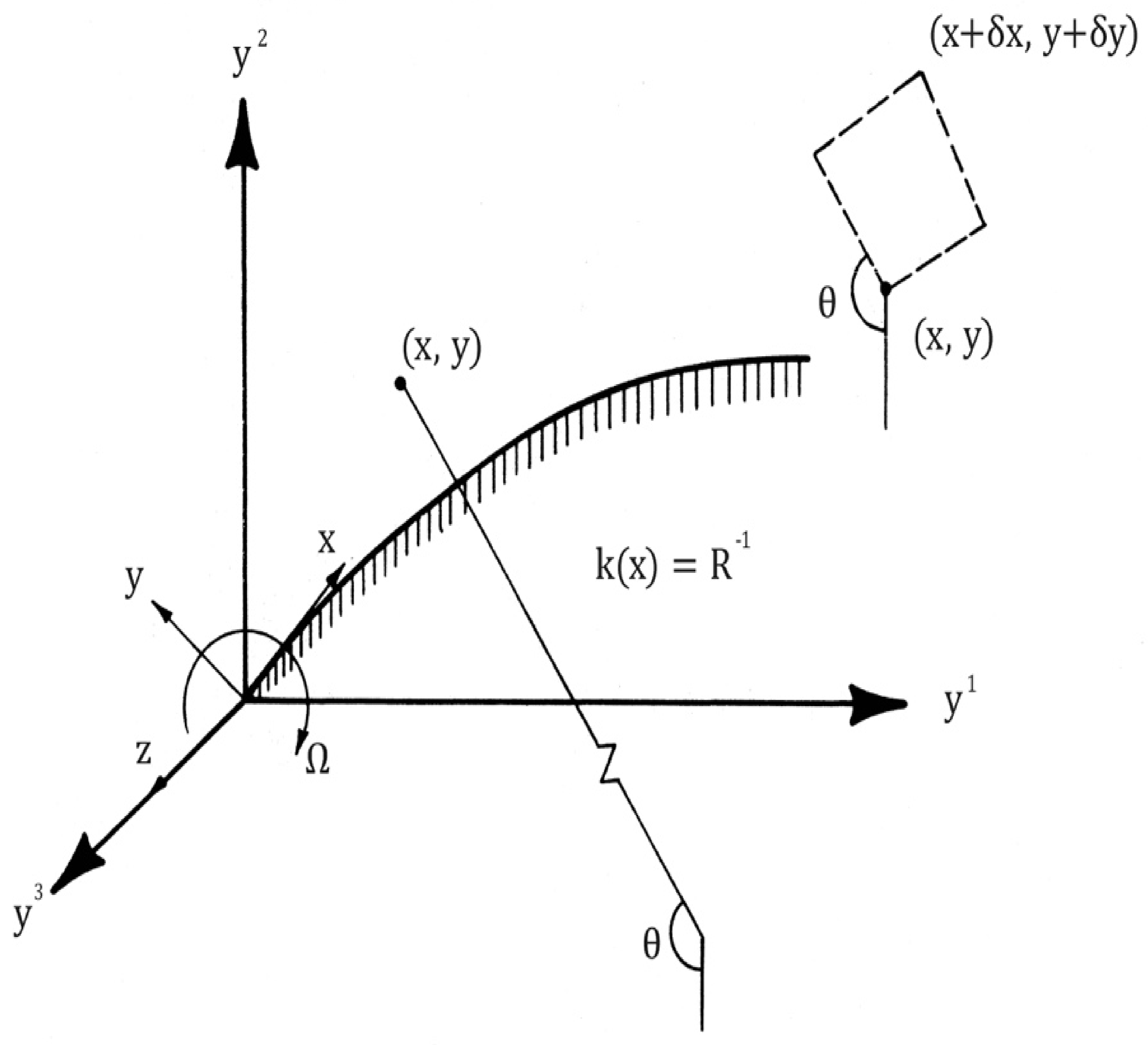
The coordinate system is assumed to be fixed to the surface and obeys the right-hand rule. Therefore, the centrifugal force due to rotation can be absorbed into the mean pressure gradient term. The overbars represent ensemble averages and the lower-case terms, ${\mathrm{u}}_{\mathrm{j}}, \mathsf{\theta },$ etc. are the fluctuating components of the velocity and temperature. These variables are governed by the following equations,

$$\frac{\partial {\mathrm{u}}_{\mathrm{i}}}{\partial {\mathrm{x}}_{\mathrm{i}}}=0,$$

(5)

$$\frac{\partial {\mathrm{u}}_{\mathrm{j}}}{\partial \mathrm{t}} + \frac{\partial }{\partial {\mathrm{x}}_{\mathrm{k}}}\left({\mathrm{U}}_{\mathrm{k}}{\mathrm{u}}_{\mathrm{j}}+ {\mathrm{U}}_{\mathrm{j}}{\mathrm{u}}_{\mathrm{k}}+ {\mathrm{u}}_{\mathrm{k}}{\mathrm{u}}_{\mathrm{j}}- \overline{{\mathrm{u}}_{\mathrm{k}}{\mathrm{u}}_{\mathrm{j}}}\right) + 2{\mathsf{ϵ}}_{\mathrm{jlm}}{\mathsf{\Omega }}_{\mathrm{k}}{\mathrm{u}}_{\mathrm{l}} =- \frac{\partial \mathrm{p}}{\partial {\mathrm{x}}_{\mathrm{j}}} + \nu {\nabla }^2{\mathrm{u}}_{\mathrm{j}},$$

(6)

$$\frac{\partial \mathsf{\theta }}{\partial \mathrm{t}} + \frac{\partial }{\partial {\mathrm{x}}_{\mathrm{k}}} \left({\mathrm{Tu}}_{\mathrm{k}} + {\mathrm{U}}_{\mathrm{k}}\mathsf{\theta } + {\mathrm{u}}_{\mathrm{k}}\mathsf{\theta } - \overline{{\mathrm{u}}_{\mathrm{k}}\mathsf{\theta }}\right)={\sigma }_{\mathrm{T}}{\nabla }^2\mathsf{\theta },$$

(7)

Since the mean flow Equations (2)–(4) involve the Reynolds stress $\overline{{\mathrm{u}}_{\mathrm{i}}{\mathrm{u}}_{\mathrm{j}}}$ and the heat flux $\overline{{\mathrm{u}}_{\mathrm{i}}\mathsf{\theta }}$ terms, their closure is made possible by introducing transport equations for these terms. These three equations are deduced from Equations (6) and (7). The final equations for $\overline{{\mathrm{u}}_{\mathrm{i}}{\mathrm{u}}_{\mathrm{j}}} \mathrm{and} \overline{{\mathrm{u}}_{\mathrm{j}}\mathsf{\theta }}$ are given below [24] as:

$$\begin{array}{c}\frac{\partial \overline{{\mathrm{u}}_{\mathrm{i}}{\mathrm{u}}_{\mathrm{j}}}}{\partial \mathrm{t}} + \frac{\partial }{\partial {\mathrm{x}}_{\mathrm{k}}} \left[{\mathrm{U}}_{\mathrm{k}}\overline{ {\mathrm{u}}_{\mathrm{i}}{\mathrm{u}}_{\mathrm{j}}} + \overline{{\mathrm{u}}_{\mathrm{k}}{\mathrm{u}}_{\mathrm{i}}{\mathrm{u}}_{\mathrm{j}}} - \nu \frac{\partial \overline{{\mathrm{u}}_{\mathrm{i}}{\mathrm{u}}_{\mathrm{j}}}}{\partial {\mathrm{x}}_{\mathrm{k}}}\right] + \frac{\partial }{\partial {\mathrm{x}}_{\mathrm{k}}}\left[\overline{{\mathrm{pu}}_{\mathrm{i}}}{\delta }_{\mathrm{jk}} + \overline{{ \mathrm{pu}}_{\mathrm{j}}}{\delta }_{\mathrm{ik}}\right]\\ =- \overline{{\mathrm{u}}_{\mathrm{i}}{\mathrm{u}}_{\mathrm{k}}}\frac{\partial {\mathrm{U}}_{\mathrm{j}}}{\partial {\mathrm{x}}_{\mathrm{k}}}- \overline{{\mathrm{u}}_{\mathrm{j}}{\mathrm{u}}_{\mathrm{k}}}\frac{\partial {\mathrm{U}}_{\mathrm{i}}}{\partial {\mathrm{x}}_{\mathrm{k}}}- 2\left[{\mathsf{ϵ}}_{\mathrm{ilm}}{\mathsf{\Omega }}_{\mathrm{l}}\overline{{\mathrm{u}}_{\mathrm{m}}{\mathrm{u}}_{\mathrm{j}}} + {\mathsf{ϵ}}_{\mathrm{jlm}}{\mathsf{\Omega }}_{\mathrm{l}}\overline{{\mathrm{u}}_{\mathrm{m}}{\mathrm{u}}_{\mathrm{i}}}\right]\\ + \overline{\mathrm{p}\left(\frac{\partial {\mathrm{u}}_{\mathrm{i}}}{\partial {\mathrm{x}}_{\mathrm{j}}} + \frac{\partial {\mathrm{u}}_{\mathrm{j}}}{\partial {\mathrm{x}}_{\mathrm{i}}}\right)}- 2\nu \overline{\frac{\partial {\mathrm{u}}_{\mathrm{i}}}{\partial {\mathrm{x}}_{\mathrm{k}}} \frac{\partial {\mathrm{u}}_{\mathrm{j}}}{\partial {\mathrm{x}}_{\mathrm{k}}}},\end{array}$$

(8)

$$\begin{gathered} \frac{\partial \overline{{\mathrm{u}}_{\mathrm{j}}\mathsf{\theta }}}{\partial \mathrm{t}} + \frac{\partial }{\partial {\mathrm{x}}_{\mathrm{k}}} \left[{ \mathrm{U}}_{\mathrm{k}}\overline{{\mathrm{u}}_{\mathrm{j}}\mathsf{\theta }} + \overline{{\mathrm{u}}_{\mathrm{k}}{\mathrm{u}}_{\mathrm{j}}\mathsf{\theta }} - {\sigma }_{\mathrm{T}}\overline{{\mathrm{u}}_{\mathrm{j}}\frac{\partial \mathsf{\theta }}{\partial {\mathrm{x}}_{\mathrm{k}}}} - \nu \overline{\mathsf{\theta }\frac{\partial {\mathrm{u}}_{\mathrm{j}}}{\partial {\mathrm{x}}_{\mathrm{k}}}} \right] + \frac{\partial \overline{\mathrm{p}\mathsf{\theta }}}{\partial {\mathrm{x}}_{\mathrm{j}}} = \\ - \overline{{\mathrm{u}}_{\mathrm{j}}{\mathrm{u}}_{\mathrm{k}}}\frac{\partial \mathrm{T}}{\partial {\mathrm{x}}_{\mathrm{k}}}- \overline{{\mathsf{\theta }\mathrm{u}}_{\mathrm{k}}}\frac{\partial {\mathrm{U}}_{\mathrm{j}}}{\partial {\mathrm{x}}_{\mathrm{k}}}- 2{\mathsf{ϵ}}_{\mathrm{jlm}}{\mathsf{\Omega }}_{\mathrm{l}}\overline{{\mathrm{u}}_{\mathrm{m}}\mathsf{\theta }} + \overline{\mathrm{p}\frac{\partial \mathsf{\theta }}{\partial {\mathrm{x}}_{\mathrm{j}}}}- \left({\sigma }_{\mathrm{T}}+ \nu \right)\overline{\frac{\partial {\mathrm{u}}_{\mathrm{j}}}{\partial {\mathrm{x}}_{\mathrm{k}}} \frac{\partial \mathsf{\theta }}{\partial {\mathrm{x}}_{\mathrm{k}}}}, \end{gathered}$$

(9)

Note that in writing down Equations (8) and (9), all the advection and diffusion terms are grouped into the left-hand side of the equations. Consequently, if these terms are assumed to be negligible, only the pressure–strain correction and the dissipation terms need modelling.

3. Modelling Assumptions and the Simplified Transport Equations

The equations that govern the transport of the Reynolds stress $-\overline{{\mathrm{u}}_{\mathrm{i}}{\mathrm{u}}_{\mathrm{j}}}$, i.e., Equation (8), form an indeterminate set of equations because higher order moments, such as $\overline{{\mathrm{u}}_{\mathrm{i}}{\mathrm{u}}_{\mathrm{j}}{\mathrm{u}}_{\mathrm{k}}}$ and $\overline{{\mathrm{u}}_{\mathrm{k}}{\mathrm{u}}_{\mathrm{j}}\mathsf{\theta }}$, are present. Furthermore, the energy redistribution term, or more precisely the pressure–velocity correlation term $\partial \left(\overline{{\mathrm{pu}}_{\mathrm{i}}}{\delta }_{\mathrm{jk}} + \overline{{ \mathrm{pu}}_{\mathrm{j}}}{\delta }_{\mathrm{ik}}\right)/\partial {\mathrm{x}}_{\mathrm{k}}$ and the viscous dissipation term 2$\nu \overline{\left\{\left(\partial {\mathrm{u}}_{\mathrm{i}}/\partial {\mathrm{x}}_{\mathrm{k}}\right)\left(\partial {\mathrm{u}}_{\mathrm{j}}/\partial {\mathrm{x}}_{\mathrm{k}}\right)\right\}}$ are not known. In order to reduce the Reynolds stress equations to a closed set of equations where the dependent variables are the Reynolds stresses, suitable modelling of the pressure–velocity correlation and the dissipation terms are necessary. In view of this, further assumptions need to be introduced to simplify the Reynolds stress equations. The approach used follows closely that adopted by Mellor [25] to treat atmospheric surface layer, and by So [26,27] to model curvature and swirl effect in boundary layer flows.

The first of these assumptions is local equilibrium in the turbulence field, i.e., production of turbulence energy balances viscous dissipation except in a very thin layer next to the surface. A second assumption stipulates that the advection and diffusion terms in Equation (8) are small outside of the constant flux region; thus, the only terms that need modelling are the pressure–velocity correlation and dissipation rate terms in Equation (8). Consequently, these two assumptions allow simplifications to be made in the modelling of the pressure–velocity correlation and dissipation rate terms. With these simplifications, the classical model of Rotta [28] can be justifiably used to model the pressure–velocity correlation terms, while the local small-scale isotropy hypothesis of Kolmogorov [29,30] can be adopted to model the dissipation rate terms. Finally, under these simplifications, a parallel can be drawn between the atmospheric surface layer and other boundary layers subject to the influence of external body forces. These assumptions have also been invoked by So [31] to derive a Reynolds analogy that is valid for thermal turbulent flows over rotating curved surfaces. In that analysis, the Reynolds analogy was shown to reduce exactly to the original Reynolds analogy put forward by Monin and Oboukhov [32] for the atmospheric surface layer when all external body forces other than buoyancy are essentially zero. Thus simplified, the modelled terms proposed are given by

$$- \overline{\mathrm{p}\left(\frac{\partial {\mathrm{u}}_{\mathrm{i}}}{\partial {\mathrm{x}}_{\mathrm{j}}} + \frac{\partial {\mathrm{u}}_{\mathrm{j}}}{\partial {\mathrm{x}}_{\mathrm{i}}}\right)}=-\frac{1}{6}\frac{q}{{\ell }_1}\left(\overline{{\mathrm{u}}_{\mathrm{i}}{\mathrm{u}}_{\mathrm{j}}} - {\delta }_{\mathrm{ij}}\frac{q^2}{3}\right),$$

(10)

$$- \overline{\mathrm{p}\frac{\partial \mathsf{\theta }}{\partial {\mathrm{x}}_{\mathrm{j}}}}=\frac{q}{3{\ell }_2}\overline{{\mathrm{u}}_{\mathrm{j}}\mathsf{\theta }},$$

(11)

$$2\nu \overline{\frac{\partial {\mathrm{u}}_{\mathrm{i}}}{\partial {\mathrm{x}}_{\mathrm{k}}} \frac{\partial {\mathrm{u}}_{\mathrm{j}}}{\partial {\mathrm{x}}_{\mathrm{k}}}}=\frac{2}{3} \frac{q^3}{{\mathsf{\Lambda }}_1} {\delta }_{\mathrm{ij}},$$

(12)

$$\left({\sigma }_{\mathrm{T}} + \nu \right) \overline{ \frac{\partial {\mathrm{u}}_{\mathrm{j}}}{\partial {\mathrm{x}}_{\mathrm{k}}} \frac{\partial \mathsf{\theta }}{\partial {\mathrm{x}}_{\mathrm{k}}}}=0,$$

(13)

where Equation (13) is a consequence of the fact that there is no isotropic first-order tensor. Note that in Equation (10), the effect of the mean velocity gradient on the redistribution terms is neglected as suggested by Rotta [28]. However, this contribution is put back into Equation (10) in the modelling of the atmospheric boundary layer [25]. It will be shown later that this mean velocity gradient term does have an effect on the value of ${\mathrm{a}}_1$ and should be included in Equation (10), irrespective of whether the flow is simple or complex and with or without external body force effect.

Equations (10)–(13) are substituted into Equations (8) and (9). If the flow is assumed to be statistically steady and the advection and diffusion terms are assumed to be small, then these simplifications would enable the transport equations, Equations (8) and (9), to be written in a generalized tensor form as:

$$\begin{array}{r}0 = \overline{{\mathrm{u}}^{\mathrm{k}}{\mathrm{u}}_{\mathrm{j}}} {\mathrm{U}}_{\mathrm{i}, \mathrm{k}}- \overline{{\mathrm{u}}^{\mathrm{k}}{\mathrm{u}}_{\mathrm{i}}} {\mathrm{U}}_{\mathrm{j}, \mathrm{k}}- 2 \left[{\mathsf{ϵ}}_{\mathrm{ilm}}{\mathsf{\Omega }}^{\mathrm{l}}{\mathrm{u}}^{\mathrm{m}}{\mathrm{u}}_{\mathrm{j}} + {\mathsf{ϵ}}_{\mathrm{jlm}}{\mathsf{\Omega }}^{\mathrm{l}}{\mathrm{u}}^{\mathrm{m}}{\mathrm{u}}_{\mathrm{i}}\right]\\ - \frac{q}{3{\ell }_1}\left(\overline{{\mathrm{u}}_{\mathrm{i}}{\mathrm{u}}_{\mathrm{j}}} - \frac{1}{3}{\mathrm{g}}_{\mathrm{ij}}{q}^2\right)- \frac{2}{3}{\mathrm{g}}_{\mathrm{ij}}\frac{q^3}{\mathsf{\Lambda }},\end{array}$$

(14)

$$0=- \overline{{\mathsf{\theta }\mathrm{u}}^{\mathrm{k}}}{\mathrm{U}}_{\mathrm{j}, \mathrm{k}} - \overline{{\mathrm{u}}^{\mathrm{k}}{\mathrm{u}}_{\mathrm{j}}}{\mathrm{T}}_{, \mathrm{k}} - 2{\mathsf{ϵ}}_{\mathrm{jlm}}{\mathsf{\Omega }}^{\mathrm{l}}\overline{{\mathrm{u}}^{\mathrm{m}}\mathsf{\theta }} - \frac{q}{3{\ell }_2}\overline{{\mathrm{u}}_{\mathrm{j}}\mathsf{\theta }},$$

(15)

where q and ${\mathrm{g}}_{\mathrm{ij} } \mathrm{are} \mathrm{given} \mathrm{by} q={\left(\overline{{\mathrm{u}}^{\mathrm{i}}{\mathrm{u}}_{\mathrm{i}}}\right)}^{1/2}, {\mathrm{and} \mathrm{g}}_{\mathrm{ij}}=\left(\partial {\mathrm{y}}^{\mathrm{m}}\partial {\mathrm{y}}^{\mathrm{m}}/\partial {\mathrm{x}}^{\mathrm{i}}\partial {\mathrm{x}}^{\mathrm{j}}\right)$. The component equations can be written out with respect to a curvilinear co-ordinate system fixed to the surface and obeys the right-hand rule (Figure 1). Rotation about the y³ axis is assumed to have components (0, 0, $- \mathsf{\Omega }$). If $\left\{{\mathrm{x}}^{\mathrm{i}}\right\}=\left(\mathrm{x}, \mathrm{y}, \mathrm{z}\right)$ and $\left\{{\mathrm{u}}_{\mathrm{i}}\right\}=\left(\mathrm{u}, \mathrm{v}, \mathrm{w}\right),$ then it can be shown that

$${\mathrm{g}}_{11}={\left(1 + \mathrm{Ky}\right)}^2, {\mathrm{g}}_{22}={\mathrm{g}}_{33}=1, {\mathrm{g}}_{\mathrm{ij}}=0 \mathrm{for} \mathrm{i} \ne \mathrm{j},$$

(16)

$$\mathrm{g} \equiv \det \left({\mathrm{g}}_{\mathrm{ij}}\right)={\left(1 - \mathrm{Ky}\right)}^2 \mathrm{and} \left\{{\mathrm{g}}_{\mathrm{i}\mathrm{j}}\right\}=\left[\begin{array}{c}{\left(1 + \mathrm{K}\mathrm{y}\right)}^{-2} 0 0\\ \\ 0 1 0\\ \\ 0 0 1\end{array}\right].$$

(17)

Invoking the 2-D boundary-layer approximations and assuming $2\mathsf{\Omega }\mathrm{U}$ is of the same order as ${\mathrm{KU}}^2/\left(1 + \mathrm{Ky}\right)$, then with the help of Equations (16) and (17), the component equations of the generalized tensor Equations (14) and (15) can be deduced and they are given by

$$\frac{q}{3{\ell }_1} \left(\overline{{\mathrm{u}}^2}- \frac{q^2}{3}\right) + \frac{2}{3} \frac{q^3}{{\mathsf{\Lambda }}_1} + 2 \overline{\mathrm{uv}} \frac{\partial \mathrm{U}}{\partial \mathrm{y}} + \frac{2\mathrm{KU}}{1 + \mathrm{Ky}} \overline{\mathrm{uv}}= 0,$$

(18)

$$\frac{q}{3{\ell }_1}\left(\overline{{\mathrm{v}}^2} - \frac{q^2}{3}\right) + \frac{2}{3} \frac{q^3}{{\mathsf{\Lambda }}_1} - \frac{4\mathrm{KU}}{1 + \mathrm{Ky}} \overline{\mathrm{uv}} + 4 \mathsf{\Omega } \overline{\mathrm{uv}}=0,$$

(19)

$$\frac{q}{3{\ell }_1} \left(\overline{{\mathrm{w}}^2} - \frac{q^2}{3}\right) + \frac{2}{3}\frac{q^3}{{\mathsf{\Lambda }}_1}=0,$$

(20)

$$\frac{q}{3{\ell }_1}\overline{\mathrm{uv}} + \overline{{\mathrm{v}}^2}\frac{\partial \mathrm{U}}{\partial \mathrm{y}} - \frac{\mathrm{KU}}{1 + \mathrm{Ky}}\left(2\overline{{\mathrm{u}}^2} - \overline{{\mathrm{v}}^2}\right) + 2\mathsf{\Omega } \overline{\mathrm{v}\mathsf{\theta }}=0,$$

(21)

$$\frac{1}{3}\frac{q}{{\ell }_2} \overline{\mathrm{u}\mathsf{\theta }} + \overline{\mathrm{uv}} \frac{\partial \mathrm{T}}{\partial \mathrm{y}} + \overline{ \mathrm{v}\mathsf{\theta }} \frac{\partial \mathrm{U}}{\partial \mathrm{y}} + \frac{\mathrm{KU}}{1 + \mathrm{Ky}} \overline{\mathrm{v}\mathsf{\theta }} - 2\mathsf{\Omega } \overline{\mathrm{v}\mathsf{\theta }}=0,$$

(22)

$$\frac{1}{3}\frac{q}{{\ell }_2} \overline{\mathrm{v}\mathsf{\theta }} + \overline{{\mathrm{v}}^2} \frac{\partial \mathrm{T}}{\partial \mathrm{y}} - \frac{\mathrm{KU}}{1 + \mathrm{Ky}} \overline{\mathrm{u}\mathsf{\theta }} + 2\mathsf{\Omega } \overline{\mathrm{u}\mathsf{\theta }}=0,$$

(23)

$$\overline{\mathrm{vw}}=0, \overline{\mathrm{uw}}=0, \overline{\mathrm{w}\mathsf{\theta }}=0,$$

(24)

These simplified equations are algebraic in nature and the stress components can be solved in terms of the mean flow properties. This approach has been used by So [26], and So and Mellor [33] to estimate small and large streamline curvature effects on boundary layers, respectively. It has also been applied to estimate the effect of swirl on turbulence velocity scales [27]. Furthermore, a similar approach has been used to analytically derive a Reynolds analogy for turbulent heat transfer on rotating curved surfaces by So [31]. In view of these successes, the present approach will be adopted to model the Reynolds stress equations in pursuit of analytically deriving an expression for the shear stress and the kinetic energy of turbulence, much like the equation given by Equation (1).

Equations (18)–(24) are formulated for complex turbulent thermal flows. However, they are not suitable for analyzing atmospheric boundary layers. Since the basic data used to formulate Equation (1) was collected from atmospheric boundary layers [2], it would seem logical to start the examination of Equation (1) by considering the atmospheric boundary layer first. Atmospheric boundary layer modelling has been thoroughly treated by Mellor [25], therefore, the governing equations are readily available in [25]. On the other hand, governing equations for other complex flow cases are not readily available in the literature. In view of this, the governing equations for simple turbulent flows plus other complex turbulent flows are analyzed first to see if an equivalent Equation (1) can be derived for these flows before embarking on a similar derivation for the atmospheric boundary layer. In this approach, there is no need to repeat the above exercise to deduce the simplified equations for atmospheric boundary layer; they can be drawn directly from [25]. Further, Equation (1) has been found to yield good simulation results in a one-equation modelling of jets and free mixing flows [5,6,7]; thus, the present work should demonstrate that an equation similar to Equation (1) could also be derived for axisymmetric flows. A worthy example of an axisymmetric flow with external body force is represented by a swirling flow; thus, swirling flow will also be examined as part of complex turbulent flow.

Based on this assessment, Equations (10)–(17) will form the base to deduce a simplified set of governing equations necessary for the derivation of an equation similar to Equation (1) for each of the following five cases: Case (I)—simple flow, Case (II)—curved flow, Case (III)—rotating curved flow and Case (IV)—swirling flow. As for Case (V)—atmospheric boundary layer, it will be analyzed using the simplified governing equations reported in [25]. Together, this analysis provides a firm analytical base for a one-equation turbulence model suitable for a wide variety of turbulent flows with or without external body forces present.

4. Case I—Simple Flow

The modelled equations needed for the derivation of an equivalent Equation (1) are based on the set of simplified equations given in Equations (18)–(24). For this case, the simple flow is assumed to have no rotation and no streamline curvature. Furthermore, only isothermal flow is considered. Then the relevant equations are reduced to Equations (18)–(21) with K = 0 and $\mathsf{\Omega }=0$. The co-ordinate system for these equations has already been specified in Figure 1, therefore, it is also adopted for this flow case. The Reynolds stresses are $\overline{{\mathrm{u}}^2}, \overline{{ \mathrm{v}}^2}, \overline{{ \mathrm{w}}^2} \mathrm{and} \overline{\mathrm{uv}}$, and $k= \overline{{\mathrm{u}}^2}+ \overline{{\mathrm{v}}^2}+ \overline{{\mathrm{w}}^2} =q^2/2$ is the kinetic energy of turbulence, where (u, v, w) are the fluctuating velocity components along the (x, y, z) direction, respectively. Thus, for a two-dimensional flow, the simplified Reynolds stress equations are given by:

$$\frac{q}{3{\ell }_1} \left(\overline{{\mathrm{u}}^2}- \frac{q^2}{3}\right) + \frac{2}{3} \frac{q^3}{{\mathsf{\Lambda }}_1} + 2 \overline{\mathrm{uv}} \frac{\partial \mathrm{U}}{\partial \mathrm{y}}=0,$$

(25)

$$\frac{q}{3{\ell }_1}\left(\overline{{\mathrm{v}}^2} - \frac{q^2}{3}\right) + \frac{2}{3} \frac{q^3}{{\mathsf{\Lambda }}_1}=0,$$

(26)

$$\frac{q}{3{\ell }_1} \left(\overline{{\mathrm{w}}^2} - \frac{q^2}{3}\right) + \frac{2}{3}\frac{q^3}{{\mathsf{\Lambda }}_1}=0,$$

(27)

$$\frac{q}{3{\ell }_1}\overline{\mathrm{uv}} + \overline{{\mathrm{v}}^2}\frac{\partial \mathrm{U}}{\partial \mathrm{y}}=0,$$

(28)

and $\overline{\mathrm{uw}}=\overline{\mathrm{vw}}=0$ because of symmetry, U is the mean flow along the x-direction, while ${\ell }_1$ is a length scale introduced in the modelled terms given by Equation (10) and ${\mathsf{\Lambda }}_1$ is a length scale introduced in the modelling of the dissipation rate terms in Equation (12). The above equations can be solved to give an expression each for q² and $- \overline{\mathrm{uv}}$. The algebra involved is too cumbersome to report here verbatim; however, for the sake of the other cases, the solution procedure could be briefly described below. First, Equations (25)–(27) are solved to give an expression between $- \overline{\mathrm{uv}}$, $q^2$ and $\partial \mathrm{U}/\partial \mathrm{y}$. The $- \overline{\mathrm{uv}}$ obtained is substituted into Equation (28); and with the help of Equation (26) will yield an expression between $q^2$ and $\left(\partial \mathrm{U}/\partial \mathrm{y}\right)$, which is Equation (29) given below. Once this is obtained, Equations (26), (28) and (29) can be used to deduce an equation for $- \overline{\mathrm{uv}}$, the final form thus obtained is given in Equation (30).

$$q^2={\mathsf{\Lambda }}_1^2 \left[\mathsf{\gamma }\left(1 - 6\mathsf{\gamma }\right)\right] {\left(\frac{\partial \mathrm{U}}{\partial \mathrm{y}}\right)}^2,$$

(29)

$$- \overline{\mathrm{uv}}=\left[\mathsf{\gamma }\left(1 - 6\mathsf{\gamma }\right)\right]{ }^{1/2}\left\{q^2\right\},$$

(30)

where $\mathsf{\gamma }={\ell }_1/{\mathsf{\Lambda }}_1$. Therefore, the relation between $\tau /\rho \left( or - \overline{\mathrm{uv}} \right)$ and $q^2/2$ follows naturally from Equation (30) and can be written in a form similar to Equation (1), or:

$$\frac{\tau }{\rho }=2 {\left[\mathsf{\gamma }\left(1 - 6\mathsf{\gamma }\right)\right]}^{1/2}\left(q^2/2\right).$$

(31)

Comparing Equation (1) with Equation (29) gives the following expression for ${\mathrm{a}}_1$,

$${\mathrm{a}}_1=2 {\left[\mathsf{\gamma }\left(1 - 6\mathsf{\gamma }\right)\right]}^{1/2},$$

(32)

which is only dependent on the model constants introduced in Equations (10) and (12). From the work of Mellor [25] and So [26,27], it is known that ${\ell }_1$ and ${\mathsf{\Lambda }}_1$ are proportional to a master length scale $\ell$. These constants were determined from neutral boundary layers and grid-generated, homogeneous turbulent flows. They are found to work well for a wide variety of flows including curved shear flows and atmospheric boundary layers; as a result, $\mathsf{\gamma }$ = 0.052 is obtained. With this value for $\mathsf{\gamma }$, Equation (32) yields ${\mathrm{a}}_1= 0.378$. With the constants thus determined, Equation (31) reduces to

$$\frac{\tau }{\rho }=0.378 \left(q^2/2\right),$$

(33)

which is Equation (1) with a different ${\mathrm{a}}_1$. The case for the atmospheric boundary layer will be analyzed later in the paper. Once that is accomplished, the similarity and difference between these two cases can be identified and analyzed in detail.

This analytical derivation shows that Equation (1) should be interpreted as an equation for simple flow rather than an equation for the atmospheric boundary layer. Furthermore, this is the reason why the work of Laster [4], Lee and Harsha [5] and Harsha and Lee [6,7,8] yield good results in their use of Equation (1) to simulate free mixing layers and free shear flows without body force effects. Applications of Equation (1) to model boundary layers, both incompressible and compressible [9,10,11], and free shear flows [12] also yield good simulation results. Together, these studies lend evidence to support Equation (1) being more valid for flows without density stratification rather than for atmospheric boundary layer as suggested by Nevzgljadov [2].

In summary, it has been shown that Equation (1) can be derived from Equations (23)–(26) and ${\mathrm{a}}_1$ thus determined is about 26% higher than the empirical value deduced by Bradshaw et al. [9], and Harsha and Lee [8]. This result shows that ${\mathrm{a}}_1$ is a true constant because it only depends on the model constants invoked in the pressure–velocity correlation and dissipation rate terms. Therefore, Equation (1) can be used to simulate a wide range of 2-D turbulent shear flows without any external body force present. This analytical approach is then extended to treat flows with body force effects in subsequent sections. In the following, curvature effect will be attempted first; this is followed by rotating cured flow and swirling flow. Finally, an attempt is made to derive an equivalent of Equation (1) for atmospheric boundary layer. It is hoped that, through this systematic treatment, Equation (1) and its validity and viability for atmospheric boundary layer could be explored thoroughly.

5. Case II—Curved Flow

The effect of streamline curvature on 2-D flows due either to surface curvature, system rotation, separately or in combination, have been investigated by So [26,31], and So and Mellor [33]. The governing equations for the present analysis can be deduced from those given in [30] or directly from Equations (18)–(24). Since a curvilinear orthogonal co-ordinate system fixed to the rotating surface has been adopted by So [30] to analyze Reynlds analogy and turbulent heat transfer on turbine blades, the coordinate system used in [31] and shown in Figure 1 is adopted. The rotation about the y³ or z-axis is assumed to have components (0, 0, −$\mathsf{\Omega }$) for the rotating blade case. In the present case, the y-axis is normal to the x–z plane, while surface curvature defined as K = 1/R also lies on the x–z plane. Therefore, the equations derived for rotating curved flow can be used for the curved flow case by simply setting the rotational speed $\mathsf{\Omega }$ to zero because the blade is stationary. For the present case, i.e., a stationary blade, $\mathsf{\Omega }$ = 0, then the governing equations can be deduced from Equations (18)–(24) by setting $\mathsf{\Omega }$ = 0. In the following equations, the turbulent shear stress $\left(- \overline{\mathrm{uv}}\right)$ is replaced by $\tau /\rho$ and the simplified component equations for the Reynolds stresses, after invoking 2-D boundary layer approximations and assuming production balances dissipation in the constant flux region, can be written as:

$$\frac{1}{3}\frac{q}{{\ell }_1}\left(\overline{{\mathrm{u}}^2} - \frac{q^2}{3}\right) + \frac{2}{3}\frac{q^3}{\mathsf{\Lambda }} - 2\frac{\tau }{\rho }\frac{\partial \mathrm{U}}{\partial \mathrm{z}} - \frac{2\mathrm{KU}}{1 + \mathrm{Ky}}\frac{\tau }{\rho }=0,$$

(34)

$$\frac{1}{3}\frac{q}{{\ell }_1}\left(\overline{{\mathrm{v}}^2} - \frac{q^2}{3}\right) + \frac{2}{3}\frac{q^3}{\mathsf{\Lambda }} + \frac{4\mathrm{KU}}{1 + \mathrm{Ky}}\frac{\tau }{\rho }=0,$$

(35)

$$\frac{1}{3}\frac{q}{{\ell }_1}\left(\overline{{\mathrm{w}}^2} - \frac{q^2}{3}\right) + \frac{2}{3}\frac{q^3}{\mathsf{\Lambda }} =0,$$

(36)

$$\frac{1}{3}\frac{q}{{\ell }_1}\frac{\tau }{\rho } - \overline{{\mathrm{v}}^2}\frac{\partial \mathrm{U}}{\partial \mathrm{y}} + \frac{\mathrm{KU}}{1 + \mathrm{Ky}}\left(2\overline{{\mathrm{u}}^2} - \overline{{\mathrm{v}}^2}\right)=0,$$

(37)

As before, these equations can be solved to give the following equations for $q^2 \mathrm{and} \tau /\rho$:

$$q^2={\mathsf{\Lambda }}_1^2\frac{{\mathrm{a}}_1^2}{4} \left(1 - \frac{1}{2}\mathsf{\beta }{\mathrm{Ri}}_{\mathrm{C}}\right){\left(\frac{\partial \mathrm{U}}{\partial \mathrm{y}} - \frac{\mathrm{KU}}{1 + \mathrm{Ky}}\right)}^2,$$

(38)

$$\frac{\tau }{\rho }={\mathrm{a}}_1{\left(1 - \frac{1}{2} \mathsf{\beta }{\mathrm{Ri}}_{\mathrm{C}}\right)}^{\frac{1}{2}}\left(q^2/2\right),$$

(39)

where $\mathsf{\beta }=72\mathsf{\gamma }/\left(1 - 6\mathsf{\gamma }\right)$ has been substituted. In these equations, ${\mathrm{a}}_1$ is again given by Equation (32). Since the gradient Richardson number ${\mathrm{Ri}}_{\mathrm{C}}$ for curved flow is defined as the ratio (body force created by streamline curvature)/(typical inertial force). It has been shown to be ${\mathrm{Ri}}_{\mathrm{C}}= {\mathrm{S}}_{\mathrm{C}}\left(1 + {\mathrm{S}}_{\mathrm{C}}\right)$ by So [31], where ${\mathrm{S}}_{\mathrm{C}}$ for curved flow only is given by

$${\mathrm{S}}_{\mathrm{C}}=\left(\frac{2\mathrm{KU}}{1 + \mathrm{Ky}}\right)/\left(\frac{\partial \mathrm{U}}{\partial \mathrm{y}} - \frac{\mathrm{KU}}{1 + \mathrm{Ky}}\right).$$

(40)

Equations (38) and (39) can be combined to give an equation for the shear stress and kinetic energy of turbulence. The result is:

$$\frac{\tau }{\rho }={\mathrm{a}}_1{\left[1 - \frac{1}{4}\mathsf{\beta }{\mathrm{Ri}}_{\mathrm{C}}\right]}^{1/2}\left(q^2/2\right).$$

(41)

This equation is similar to Equation (1). However, ${\mathrm{a}}_1$ is modified by an expression that is a function of the gradient Richard number, ${\mathrm{Ri}}_{\mathrm{C}}$. For ${\mathrm{Ri}}_{\mathrm{C}}\ll$ 1, Equation (41) reduces to

$$\frac{\tau }{\rho }=0.378 \left[1 - 1.36{\mathrm{Ri}}_{\mathrm{C}}\right] \left(q^2/2\right),$$

(42)

where ${\mathrm{a}}_{1 }$= 0.378, $\mathsf{\gamma }={\ell }_1/{\mathsf{\Lambda }}_1$ = 0.052 and $\mathsf{\beta }=72\mathsf{\gamma }/\left(1 - 6\mathsf{\gamma }\right)=5.44$ have been substituted. This shows that ${\mathrm{a}}_{1 }$ does not change with flow type. In addition, it is observed that external body force gives rise to a multiplying function of ${ \mathrm{Ri}}_{\mathrm{C}}$ for ${\mathrm{a}}_{1 }$ in Equation (1). This case shows that streamline curvature will give rise to a modification of the constant ${\mathrm{a}}_{1 }$. Therefore, it could be speculated that an equivalent Equation (1) for atmospheric boundary layer would be more in line with Equation (41) than with Equation (1).

6. Case III—Rotating Curved Flow

The thermal rotating curved flow case has been treated by So [31]. For the present case, the flow is assumed to be isothermal and the coordinate system adopted is shown in Figure 1. In this figure, z is the axis of rotation and $\mathsf{\Omega }$ is the rotational speed. Equations (18)–(24) can be simplified to give the component equations for the Reynolds stresses after invoking 2-D boundary layer approximations and assuming production balances dissipation in the constant flux region. The resultant equations can be written as:

$$\frac{1}{3}\frac{q}{{\ell }_1}\left(\overline{{\mathrm{u}}^2} - \frac{q^2}{3}\right) + \frac{2}{3}\frac{q^3}{\mathsf{\Lambda }} - 2\frac{\tau }{\rho }\frac{\partial \mathrm{U}}{\partial \mathrm{y}} - \frac{2\mathrm{KU}}{1 + \mathrm{Ky}}\frac{\tau }{\rho } + 4\mathsf{\Omega }\frac{\tau }{\rho }=0,$$

(43)

$$\frac{1}{3} \frac{q}{{\ell }_1}\left(\overline{{\mathrm{v}}^2} - \frac{q^2}{3}\right) + \frac{2}{3} \frac{q^3}{\mathsf{\Lambda }} + \frac{4\mathrm{KU}}{1 + \mathrm{Ky}} \frac{\tau }{\rho } - 4\mathsf{\Omega }\frac{\tau }{\rho }=0,$$

(44)

$$\frac{1}{3}\frac{q}{{\ell }_1}\left(\overline{{\mathrm{w}}^2} - \frac{q^2}{3}\right) + \frac{2}{3}\frac{q^3}{\mathsf{\Lambda }}=0,$$

(45)

$$\frac{1}{3}\frac{q}{{\ell }_1}\frac{\tau }{\rho } - \overline{{\mathrm{v}}^2}\frac{\partial \mathrm{U}}{\partial \mathrm{y}} + \frac{\mathrm{KU}}{1 + \mathrm{Ky}}\left(2\overline{{\mathrm{u}}^2} - \overline{{\mathrm{v}}^2}\right) - 2\mathsf{\Omega }\left(\overline{{\mathrm{u}}^2} - \overline{{\mathrm{v}}^2}\right)=0,$$

(46)

where $\overline{\mathrm{vw}}=0, \mathrm{and} \overline{\mathrm{uw}}=0$. For the sake of convenience in deriving an equivalent Equation (1), $\tau /\rho$ has been substituted for $-\overline{\mathrm{uv}}$ in writing down Equations (43)–(46). Furthermore, it has been assumed that $2\mathsf{\Omega }\mathrm{U}$ and ${\mathrm{K}\mathrm{U}}^2/\left(1 + \mathrm{Ky}\right)$ are of the same order. Therefore, solving these equations yield the following expressions for $q^2$ and $\tau /\rho =-\overline{\mathrm{uv}}$, respectively:

$$q^2={\mathsf{\Lambda }}_1^2\frac{{\mathrm{a}}_1^2}{4}\left(1 - \frac{1}{2}\mathsf{\beta }{\mathrm{Ri}}_{\mathrm{RC}}\right){\left(\frac{\partial \mathrm{U}}{\partial \mathrm{y}} - \frac{\mathrm{KU}}{1 + \mathrm{Ky}}\right)}^2,$$

(47)

$$\frac{\tau }{\rho }=-\overline{\mathrm{uv}}{ = \mathrm{a}}_1{\left(1 - \frac{1}{2}\mathsf{\beta }{\mathrm{Ri}}_{\mathrm{RC}}\right)}^{\frac{1}{2}}\left(q^2/2\right),$$

(48)

where $\mathsf{\beta }=72\mathsf{\gamma }/\left(1 - 6\mathsf{\gamma }\right)$ is again obtained for this case, and the gradient Richardson number ${\mathrm{Ri}}_{\mathrm{RC}}$ for rotating curved flow is defined as

$${\mathrm{Ri}}_{\mathrm{RC}}={\mathrm{S}}_{\mathrm{RC}}\left(1 + {\mathrm{S}}_{\mathrm{RC}}\right),$$

(49)

with ${\mathrm{S}}_{\mathrm{RC}}$ given by

$${\mathrm{S}}_{\mathrm{RC}}=\left(\frac{2\mathrm{KU}}{1+ \mathrm{Ky}} - 2\mathsf{\Omega }\right)/\left(\frac{\partial \mathrm{U}}{\partial \mathrm{y}} - \frac{\mathrm{KU}}{1 + \mathrm{Ky}}\right)$$

(50)

Here, ${\mathrm{a}}_1$ is again given by Equation (32), while ${\mathrm{Ri}}_{\mathrm{RC}}$ is now defined to include both rotation and streamline curvature effects. From these results, it can be seen that the equivalent Equation (1) for rotating curved flow is given by Equation (48). These results show that the number and type of external body force present do not change the overall form of the equivalent Equation (1). The form remains the same; however, based on the Richardson number proposed by Monin and Oboukhov [32], the gradient Richardson number for rotating curved flow is now given by Equations (49) and (50). Since the modifying factor for ${\mathrm{a}}_1$ depends on the gradient Richardson number, it will change as the nature of the external body force changes. These changes do not affect the constants in Equation (48), therefore, $\mathsf{\gamma } \mathrm{and} \mathsf{\beta }$ are again given by 0.052 and 5.44, respectively. If this behavior holds true for other external body forces, the modifier of ${\mathrm{a}}_1$ for flows with different external body forces would essentially have the same form; however, the Richardson number function might be completely different.

7. Case IV—Swirling Flow

The effect of swirl on $\tau$ can also be examined in the same way. In this case, the flow is assumed to be axisymmetric and swirl around the x-axis (Figure 2). Since swirl effect has been previously examined by So [27], only the final equations for the components of the Reynolds stresses are given here. This swirling flow is akin to a 3-D shear flow. However, the following additional assumptions are required to further simplify the component equations. First, the flow is assumed to be statistically steady, the advection and diffusion terms are taken to be small by invoking boundary layer approximations and the local equilibrium assumption. The resultant component equations are written with respect to a (x, r, $\varphi$) coordinate system shown in Figure 2. The velocity components along the coordinate axis (x, r, $\varphi$) are given by (u, v, w), respectively. Details of the derivation of the Reynolds stress component equations can be found in [27]; therefore, for brevity’s sake, only the final set of equations is reproduced here to facilitate the derivation of the equation between the turbulent shear stress and the kinetic energy of turbulence. The Reynolds stress component equations are [27]:

$$- \frac{q}{3{\ell }_1}\left(\overline{{\mathrm{u}}^2} - \frac{q^2}{3}\right) - \frac{2}{3}\frac{q^3}{\mathsf{\Lambda }} - 2\overline{\mathrm{uv}}\frac{\partial \mathrm{U}}{\partial \mathrm{r}}=0,$$

(51)

$$- \frac{q}{3{\ell }_1}\left(\overline{{\mathrm{v}}^2} - \frac{q^2}{3}\right) - \frac{2}{3}\frac{q^3}{\mathsf{\Lambda }} + 4\overline{\mathrm{vw}}\frac{\mathrm{W}}{\mathrm{r}}=0,$$

(52)

$$- \frac{q}{3{\ell }_1} \left(\overline{{\mathrm{w}}^2} - \frac{q^2}{3}\right) - \frac{2}{3}\frac{q^3}{\mathsf{\Lambda }} - 4\overline{\mathrm{vw}}\frac{\mathrm{W}}{\mathrm{r}} - 2\overline{\mathrm{vw}}\left(\frac{\partial \mathrm{W}}{\partial \mathrm{r}} - \frac{\mathrm{W}}{\mathrm{r}}\right)=0,$$

(53)

$$- \frac{q}{3{\ell }_1}\overline{\mathrm{uv}} - \overline{{\mathrm{v}}^2}\frac{\partial \mathrm{U}}{\partial \mathrm{r}} + 2\overline{\mathrm{uw}} \frac{\mathrm{W}}{\mathrm{r}}=0,$$

(54)

$$- \frac{q}{3{\ell }_1}\overline{\mathrm{vw}} - \overline{{\mathrm{v}}^2}\left(\frac{\partial \mathrm{W}}{\partial \mathrm{r}} - \frac{\mathrm{W}}{\mathrm{r}}\right) + 2\left(\overline{{\mathrm{w}}^2} - \overline{{\mathrm{v}}^2}\right)\frac{\mathrm{W}}{\mathrm{r}}=0,$$

(55)

$$- \frac{q}{3{\ell }_1}\overline{\mathrm{uw}} - \overline{ \mathrm{vw}}\frac{\partial \mathrm{U}}{\partial \mathrm{r}} - \overline{\mathrm{uv}} \left(\frac{\partial \mathrm{W}}{\partial \mathrm{r}} - \frac{\mathrm{W}}{\mathrm{r}}\right) - 2\overline{\mathrm{uv}}\frac{\mathrm{W}}{\mathrm{r}}=0,$$

(56)

Solving Equations (51)–(56) yield the following relations for $q^2, -\overline{\mathrm{uv}} \mathrm{and}-\overline{\mathrm{vw}}$:

$$q^2 ={ \mathsf{\Lambda }}_1^2 \frac{{\mathrm{a}}_1^2}{4} {\mathrm{Z}}_1\left({\mathrm{Ri}}_{\mathrm{S}}\right)\left[{\left(\frac{\partial \mathrm{U}}{\partial \mathrm{r}}\right)}^2+ {\left(\frac{\partial \mathrm{W}}{\partial \mathrm{r}} - \frac{\mathrm{W}}{\mathrm{r}}\right)}^2\right]$$

(57)

$$\frac{{\tau }_{\mathrm{r}\mathrm{x}}}{\rho }=-\overline{\mathrm{uv}}={\mathrm{a}}_1\mathrm{H}\left({\mathrm{Ri}}_{\mathrm{S}}\right)\left(q^2/2\right)$$

(58a)

$$\mathrm{where} \mathrm{H}\left({\mathrm{Ri}}_{\mathrm{S}}\right)=\left\{\frac{{\mathrm{Z}}_1^{1/2}}{{\mathrm{Z}}_1 + \left(1/2\right)\mathsf{\beta }{\mathrm{Ri}}_{\mathrm{S}}}\right\}\left[\frac{{\mathrm{Z}}_1+ \frac{1}{2}\mathsf{\beta }{\mathrm{Ri}}_{\mathrm{S}}+ {\sigma }_1^2\left({\mathrm{Z}}_1+ \frac{1}{2}{\mathsf{\beta }\mathrm{Ri}}_{\mathrm{S}}-1\right)}{{\left(1 + {\sigma }_1\right)}^{1/2}}\right],$$

(58b)

$$\frac{{\tau }_{\mathrm{r}\varphi }}{\rho }=- \overline{\mathrm{vw}}={\mathrm{a}}_1\mathrm{G}\left({\mathrm{Ri}}_{\mathrm{S}}\right)\left(q^2/2\right)$$

(59a)

$$\mathrm{where} \mathrm{G}\left({\mathrm{Ri}}_{\mathrm{S}}\right)=\left[\frac{{\mathrm{Z}}_1^{1/2}}{{\mathrm{Z}}_1 + \frac{1}{2} \mathsf{\beta } {\mathrm{Ri}}_{\mathrm{S}}}\right] \left[\frac{{\sigma }_1}{{\left(1 + {\sigma }_1^2\right)}^{1/2}}\right].$$

(59b)

The equation for $-\overline{\mathrm{uv}}$ is given by Equation (58a), where, for the sake of brevity, a function $\mathrm{H}\left({\mathrm{Ri}}_{\mathrm{S}}\right)$ defined in Equation (58b) is introduced. Similarly, the equation for $-\overline{\mathrm{vw}}$, given in Equation (59a), is written in terms of a function $\mathrm{G}\left({\mathrm{Ri}}_{\mathrm{S}}\right)$, which is defined in Equation (59b). The other symbols $\mathsf{\beta }, {\mathrm{Ri}}_{\mathrm{S}}, {\mathrm{Z}}_1\left({\mathrm{Ri}}_{\mathrm{S}}\right), \sigma \mathrm{and} {\sigma }_1$ are defined by the following expressions:

$$\mathsf{\beta }=72\mathsf{\gamma }{\left(1 - 6\mathsf{\gamma }\right)}^{-1},$$

(60)

$${\mathrm{Ri}}_{\mathrm{S}}=\frac{2\frac{\mathrm{W}}{\mathrm{r}}\left(\frac{\partial \mathrm{W}}{\partial \mathrm{r}} - \frac{\mathrm{W}}{\mathrm{r}}\right)}{{\left(\frac{\partial \mathrm{U}}{\partial \mathrm{r}}\right)}^2 + {\left(\frac{\partial \mathrm{W}}{\partial \mathrm{r}} - \frac{\mathrm{W}}{\mathrm{r}}\right)}^2},$$

(61)

$${\mathrm{Z}}_1\left({\mathrm{Ri}}_{\mathrm{S}}\right)=1 - \frac{5}{8}{\mathsf{\beta }\mathrm{Ri}}_{\mathrm{S}} + {\left[{\left(1 - \frac{3}{8}{\mathsf{\beta }\mathrm{Ri}}_{\mathrm{S}}\right)}^2 + \frac{3}{2}{\mathsf{\beta }\mathrm{Ri}}_{\mathrm{S}}^2 {\sigma }^2\right]}^{\frac{1}{2}},$$

(62)

$$\sigma =\left(\partial \mathrm{U}/\partial \mathrm{r}\right)/\left(\frac{\partial \mathrm{W}}{\partial \mathrm{r}} + \frac{\mathrm{W}}{\mathrm{r}}\right),$$

(63)

$${\sigma }_1=\left(\frac{\partial \mathrm{W}}{\partial \mathrm{r}} - \frac{\mathrm{W}}{\mathrm{r}}\right)/\left(\partial \mathrm{U}/\partial \mathrm{r}\right),$$

(64)

where W is the mean swirl velocity in the $\varphi$-direction and a₁ is again given by Equation (32). In addition, ${\mathrm{Ri}}_{\mathrm{S}}$, defined in Equation (61), has the meaning of a gradient Richardson number and is the correct parameter to use to characterize swirling flows. Therefore, for swirling flows, relations similar to Equation (1) are given by Equations (58a) and (59a) for the turbulent shear stresses ${\tau }_{\mathrm{rx}} \mathrm{and} {\tau }_{\mathrm{r}\varphi }$, respectively. In the swirling flow case, the a₁ modifying functions given in Equations (58a) and (59a) assume a more complicated form compared to the simple form seen in the curved flow and rotating curved flow cases. This means that the complexity of the modifying function in the equivalent Equation (1) is greatly influenced by the complexity of the body forces, which, in turn, is influenced by the interactions of the 3-D mean field with the 3-D turbulence field. However, for the curved flow and rotating curved flow cases, the mean field is still 2-D in nature; thus, the modifying functions are relatively simple in those cases. The ratio of the shear stresses ${\tau }_{\mathrm{r}\varphi }/{\tau }_{\mathrm{r}\mathrm{x} }$ is then given by the ratio of G/H, i.e., Equation (59b) divided by Equation (58b). The result is

$$\frac{{\tau }_{\mathrm{r}\varphi }}{{\tau }_{\mathrm{rx}}}=\frac{\mathrm{G}}{\mathrm{H}}=\frac{{\sigma }_1}{{\mathrm{Z}}_1 + \frac{1}{2} {\mathsf{\beta }\mathrm{Ri}}_{\mathrm{S}} + {\sigma }_1^2\left({\mathrm{Z}}_1 + \frac{1}{2}\mathsf{\beta }{\mathrm{Ri}}_{\mathrm{S}} - 1\right)},$$

(65)

For flows with small whirl, such that $\mathrm{W}/\mathrm{r} \ll \partial \mathrm{W}/\partial \mathrm{r},$ Equation (65) reduces to

$$\frac{{\tau }_{\mathrm{r}\varphi }}{{\tau }_{\mathrm{rx}}}=\frac{\partial \mathrm{W}/\partial \mathrm{r}}{\partial \mathrm{U}/\partial \mathrm{r}},$$

(66)

which is simply a statement for isotropic eddy viscosity or mixing length for the turbulent shear stresses. The relations given by Equations (57), (58a) and (59a) have been used to predict turbulent swirling flows and the results compared favorably with measurements [27]. Therefore, if Equations (58a) and (59a) are used in conjunction with a turbulent kinetic energy equation to calculate turbulent swirling flows, improvements over the results previously obtained by So [27] can be expected because k = ($q^2/2)$ is now given by the solution of the turbulent kinetic energy equation instead of by Equation (50) alone. The present approach to model swirling flows offers an attractive alternative to the mixing length and/or the k–$\epsilon$ two equation model. It is much simpler mathematically because the model stress equations are algebraic in nature.

Furthermore, Equation (42) can be used to evaluate ${\tau }_{\mathrm{rx}}$ for swirling flows, while ${\tau }_{\mathrm{r}\varphi }$ can be determined from Equation (66) once ${\tau }_{\mathrm{rx}}$ is known. In this case, the coefficient modifying ${\mathrm{Ri}}_{\mathrm{C}}$ can still be taken as 1.36. Another point to note is that Equation (48) can also be used to relate $\tau /\rho$ to $\left(q^2/2\right)$ for flows with combined body force effects, such as buoyancy and system rotation. However, in those cases, the modifying coefficient might take on a value different from 1.36. It should be pointed out that the Richardson number function becomes more complicated for the swirling flow case. The function is no longer linear as in the former two cases; rather, it is quite nonlinear as can be discerned from Equations (58b) and (59b). This simply reflects the enhanced complications in the turbulence field of a swirling flow. In spite of this complication, the current case demonstrates that the present approach can be easily extended to analyze axisymmetric flows.

8. Case V—Atmospheric Boundary Layer

Equations (18)–(24) are not valid for atmospheric boundary layers. Due to Coriolis force, density stratification and thermal effect, the governing equations and modelling proposals are slightly different from those given in Section 2 and Section 3. Since the problem of modelling the atmospheric boundary layer has already been thoroughly treated by Mellor [25], the present study simply adopt the governing equations and turbulence models proposed in [25]. It should be pointed out that in modelling the pressure–velocity correlation terms, the present model as given in Equation (10) does not include the mean flow gradient effect on the pressure–velocity correlation. In atmospheric boundary layer modelling, due to Coriolis force, buoyancy and thermal stratification, the mean flow gradient effect would play an important role. Therefore, it is prudent to take this mean flow gradient effect into account in the modelling of the pressure–velocity correlation terms. Inclusion of this effect amounts to adding a term such as ${\mathrm{Cq}}^2\left(\partial {\mathrm{U}}_{\mathrm{i}}/\partial {\mathrm{x}}_{\mathrm{j}} + \partial {\mathrm{U}}_{\mathrm{j}}/\partial {\mathrm{x}}_{\mathrm{i}}\right)$ to Equation (10). The coordinate system adopted by Mellor [25] use the x–y plane to represent the Earth’s surface with the z-axis normal to this plane; refer to Figure 1. Therefore, the turbulent shear stress is given by $- \overline{\mathrm{uw}}$. Again, invoking the same boundary layer approximations and local equilibrium assumption to simplify the modelled equations, the resulting $\overline{{\mathrm{u}}_{\mathrm{i}}{\mathrm{u}}_{\mathrm{j}}}, \overline{ {\mathrm{u}}_{\mathrm{i}}\mathsf{\theta }} \mathrm{and} \overline{{\mathsf{\theta }}^2}$ equations in their component form can be deduced from the full set of modelled equations. After simplifications, these equations are given by Mellor [25] as

$$\frac{q}{3{\ell }_1}\left(\overline{{\mathrm{u}}^2} - \frac{q^2}{3}\right) + \frac{2}{3}\frac{q^3}{{\mathsf{\Lambda }}_1} + 2\overline{\mathrm{uw}}\frac{\partial \mathrm{U}}{\partial \mathrm{z}}=0,$$

(67)

$$\frac{q}{3{\ell }_1}\left(\overline{{\mathrm{v}}^2} - \frac{q^2}{3}\right) + \frac{2}{3}\frac{q^3}{{\mathsf{\Lambda }}_1}=0,$$

(68)

$$\frac{q}{3{\ell }_1}\left(\overline{{\mathrm{w}}^2} - \frac{q^2}{3}\right) + \frac{2}{3} \frac{q^3}{{\mathsf{\Lambda }}_1} - 2\kappa \mathrm{g} \overline{\mathrm{w}\mathsf{\theta }}=0,$$

(69)

$$\frac{q}{3{\ell }_1} \overline{\mathrm{uw}} + \left(\overline{{\mathrm{w}}^2} - \mathrm{C}{q}^2\right) \frac{\partial \mathrm{U}}{\partial \mathrm{z}} - \kappa \mathrm{g} \overline{\mathrm{u}\mathsf{\theta }}=0$$

(70)

$$\frac{q}{3{\ell }_2} \overline{\mathrm{u}\mathsf{\theta }} + \overline{\mathrm{uw}}\frac{\partial \mathrm{T}}{\partial \mathrm{r}} + \overline{\mathrm{w}\mathsf{\theta }}\frac{\partial \mathrm{U}}{\partial \mathrm{z}}=0,$$

(71)

$$\frac{q}{3{\ell }_2} \overline{\mathrm{w}\mathsf{\theta }} + \overline{{\mathrm{w}}^2} \frac{\partial \mathrm{T}}{\partial \mathrm{r}} - \kappa \mathrm{g} \overline{{\mathsf{\theta }}^2}=0,$$

(72)

$$2\overline{\mathrm{w}\mathsf{\theta }} \frac{\partial \mathrm{T}}{\partial \mathrm{z}} + \frac{2q}{{\mathsf{\Lambda }}_2}\overline{{\mathsf{\theta }}^2}=0,$$

(73)

where $\overline{\mathrm{uv}}=\overline{\mathrm{vw}}=\overline{\mathrm{v}\mathsf{\theta }}=0$, $\kappa =- {\left(\partial \rho /\partial \mathrm{T}\right)}_p/\rho$ is the coefficient of thermal expansion, T is the mean temperature, ${\ell }_2$ is a length scale introduced in Equation (11) and ${\mathsf{\Lambda }}_2$ is a length scale introduced in the modelling of the dissipation rate term in the temperature variance equation. The modelled term with ${\mathsf{\Lambda }}_2$ appears in the second term of Equation (73). Comparing this set of equations with those given in Equations (25)–(28), it can be seen that density stratifications and Coriolis force give rise to terms that reflect nonlinear effects due to Coriolis force, and density and thermal stratifications.

Again, Equations (67) to (73) can be solved for the four components of the Reynolds stress tensor, two components of heat conduction moments, and the temperature variance $\overline{{\mathsf{\theta }}^2}$ in terms of the mean flow properties. Since the present interest is in deriving a relation between shear stress and the kinetic energy of turbulence, only the results for $–\overline{\mathrm{uw}}$ and $k =q^2/2$ are given below. Omitting all algebraic details, the results are

$$q^2 ={ \mathsf{\Lambda }}_1^2\left(\frac{1}{4}{\mathrm{a}}_1^2\right)\left(1 -{ \mathsf{\beta }}_1{\mathrm{Ri}}_{\mathrm{B}}\right)\left[\sqrt{\frac{1}{4} - \frac{{\mathrm{B}}_2}{{\mathrm{B}}_1^2}} + \frac{1}{2}\right]{\left(\frac{\partial \mathrm{U}}{\partial \mathrm{z}}\right)}^2,$$

(74)

$$\frac{\tau }{\rho } =- \overline{\mathrm{uw}} = {\mathrm{a}}_1{\left(1 - {\mathsf{\beta }}_1{\mathrm{Ri}}_{\mathrm{B}}\right)}^{1/2}{\left[\sqrt{\frac{1}{4} - \frac{{\mathrm{B}}_2}{{\mathrm{B}}_1^2}} + \frac{1}{2}\right]}^{1/2}{\mathrm{F}}_{\mathrm{B}}({\mathrm{Ri}}_{\mathrm{B}})\left\{q^2/2\right\},$$

(75a)

$${\mathrm{F}}_{\mathrm{B}}\left({\mathrm{Ri}}_{\mathrm{B}}\right)= \left[1 + \frac{{\mathsf{\gamma }}_1\left(1 - 6\mathsf{\gamma }\right){\mathrm{Ri}}_{\mathrm{B}}}{3{\mathsf{\gamma }}_1\left(6\mathsf{\gamma } +{ \mathsf{\gamma }}_2\right){\mathrm{Ri}}_{\mathrm{B}} + \frac{1}{4}{\mathrm{a}}_1^2\left(1 -{ \mathsf{\beta }}_1{\mathrm{Ri}}_{\mathrm{B}}\right)\left(\sqrt{\frac{1}{4} - \frac{{\mathrm{B}}_2}{{\mathrm{B}}_1^2}} + \frac{1}{2}\right)}\right],$$

(75b)

where ${ \mathsf{\gamma }}_1,{ \mathsf{\gamma }}_2,{ \mathsf{\beta }}_1,{ \mathrm{Ri}}_{\mathrm{B}}, {\mathrm{B}}_1,{ \mathrm{B}}_2{ \mathrm{and} \mathrm{a}}_1$ are introduced to abbreviate writing and are given below as

$${\mathsf{\gamma }}_1={\ell }_2/{\mathsf{\Lambda }}_1,{ \mathsf{\gamma }}_2 ={ \mathsf{\Lambda }}_2/{\mathsf{\Lambda }}_1,$$

(76)

$${\mathsf{\beta }}_1=\frac{21{\mathsf{\gamma }\mathsf{\gamma }}_1 +{ \mathsf{\gamma }}_1 + 3{\mathsf{\gamma }}_1{\mathsf{\gamma }}_2}{\left(1 - 6\mathsf{\gamma } - 3\mathrm{C}\right)},$$

(77)

$${\mathrm{Ri}}_{\mathrm{B}}=\frac{\kappa \mathrm{g} \left(\partial \mathrm{T}/\partial \mathrm{r}\right)}{{\left(\partial \mathrm{U}/\partial \mathrm{r}\right)}^2},$$

(78)

$${\mathrm{B}}_1={\mathsf{\Lambda }}_1^2 \frac{{\mathrm{a}}_1^2}{4} \left(1 - {\mathsf{\beta }}_1{\mathrm{Ri}}_{\mathrm{B}}\right),$$

(79)

$$\begin{gathered} {\mathrm{B}}_2 = {\mathsf{\Lambda }}_1^4[ 9{\mathsf{\gamma }\mathsf{\gamma }}_1\mathrm{C} \left({\mathsf{\gamma }}_{2 }+ 6\mathsf{\gamma }\right)- 3\mathsf{\gamma }\left(1 - 6\mathsf{\gamma }\right)\left(3{\mathsf{\gamma }}_1^2 - {\mathsf{\gamma }\mathsf{\gamma }}_2\right) \\ + \left.9{\mathsf{\gamma }\mathsf{\gamma }}_1^2\left(1 + 3{\mathsf{\gamma }}_{2 } + 12\mathsf{\gamma }\right){\mathrm{Ri}}_{\mathrm{B}} \right]{\mathrm{Ri}}_{\mathrm{B}}, \end{gathered}$$

(80)

$${\mathrm{a}}_1=2 {\left[\mathsf{\gamma }\left(1 - 6\mathsf{\gamma } - 3\mathrm{C}\right)\right]}^{1/2}.$$

(81)

In these equations, ${\mathrm{Ri}}_{\mathrm{B}}$ is the gradient Richardson number for buoyant flow. Since its definition has been given by Monin and Oboukhov [32] as the ratio of the body force due to buoyancy divided by the inertial force of the buoyant flow, it is as defined in Equation (78). In addition, there is an additional term representing the effect of mean velocity gradient on the Rotta [28] model for the pressure–velocity correlation term. Therefore, the previously derived coefficient ${\mathrm{a}}_1$, as given by Equation (32), will be modified by this additional term. The new term for ${\mathrm{a}}_1$ is given by Equation (81). It can be seen that an additional term given by ($-3\mathrm{C}$) is added to the expression $\left(1 - 6\mathsf{\gamma }\right)$, a consequence of the mean velocity gradient effect.

Another observation can be made on Equations (74), (75a) and (75b). The presence of buoyant force, Coriolis force and temperature change in the atmospheric boundary layer complicates the turbulence field in the surface layer in a significant way. This complication is reflected in Equations (75a) and (75b) where the dependence on ${\mathrm{Ri}}_{\mathrm{B}}$ is nonlinear in nature. However, if ${\mathrm{Ri}}_{\mathrm{B}}$ is very small, then Equation (75b) can be approximated by one and Equation (75a) becomes quite similar to Equation (39) for the curved flow case. Even then, Equation (75a) is not similar to Equation (1), except for the case where ${\mathrm{Ri}}_{\mathrm{B}}$ is very much smaller than 1, such that it can be essentially assumed to be zero; then, Equation (1) can be recovered. In other words, Equation (1) only holds true for this limiting case. For other more complicated atmospheric conditions, Equation (1) is most likely not applicable.

For the more general case, the required relation between $\tau /\rho =- \left(\overline{\mathrm{uw}}\right)$= $\left(q^2/2\right)$ is given by Equation (75a), which can be rewritten in a short form as

$$\frac{\tau }{\rho }=- \left(\overline{\mathrm{uw}}\right) ={ \mathrm{a}}_1 \mathrm{Z}\left({\mathrm{Ri}}_{\mathrm{B}}\right) \left\{q^2/2\right\},$$

(82)

where Z$\left({\mathrm{Ri}}_{\mathrm{B}}\right)$ is defined as

$$\mathrm{Z} = \left\{{\left(1 -{ \mathsf{\beta }}_1{\mathrm{Ri}}_{\mathrm{B}}\right)}^{1/2}\left[\sqrt{\frac{1}{4} - \frac{{\mathrm{B}}_2}{{\mathrm{B}}_1^2}} + \frac{1}{2}\right]{ \mathrm{F}}_{\mathrm{B}}\left({\mathrm{Ri}}_{\mathrm{B}}\right)\right\}$$

(83)

The constant between $\tau$ and $\rho \left(q^2/2\right)$ is given by ${\mathrm{a}}_1=0.328$, if as previously assumed, $\mathsf{\gamma }=0.052 \mathrm{and} \mathrm{C}=0.056$ are adopted. Since none of the length scales introduced through the turbulence models appear explicitly in Equation (82), a length scale equation will not be required, and Equation (82) can be used in conjunction with the turbulent kinetic energy equation to define the turbulent shear field in atmospheric boundary layer.

Using the length scales adopted by Mellor [25], the two ratios given in Equation (76) take on the following values, ${\mathsf{\gamma }}_1= 0.052 \mathrm{and} {\mathsf{\gamma }}_2=0.533$. If ${\mathrm{Ri}}_{\mathrm{B}}\ll 1$, then to the first approximation, the modifying function $\mathrm{Z}\left({\mathrm{Ri}}_{\mathrm{B}}\right)$ given in Equation (82) can be simplified to

$$\mathrm{Z}\left({\mathrm{Ri}}_{\mathrm{B}}\right)=1 - {\mathsf{\beta }}_2{\mathrm{Ri}}_{\mathrm{B}},$$

(84)

with ${\mathsf{\beta }}_2=4.453$ determined from Equation (82) by assuming ${\mathrm{Ri}}_{\mathrm{B}}$ to be very small. Furthermore, $\mathsf{\gamma }= {\mathsf{\gamma }}_1= 0.052, {\mathsf{\gamma }}_2=0.533, \mathrm{C}= 0.056 \mathrm{and} {\mathsf{\beta }}_2=4.453$ can be deduced from Equation (82). With these simplifications and assuming very small ${\mathrm{Ri}}_{\mathrm{B}}$, Equation (82) reduces to

$$\frac{\tau }{\rho }=0.328 \left[1 - 4.453{\mathrm{Ri}}_{\mathrm{B}}\right]\left(q^2/2\right),$$

(85)

thus, providing a simple correction for density stratification alone. Other effects are essentially neglected.

It is now clear why Equation (1) works well in the simulations of a wide range of turbulent mixing flows and boundary layers even though it is derived using atmospheric boundary layer data [4,5,6,7,8,9,10,11,12,13,14]. For very small ${\mathrm{Ri}}_{\mathrm{B}}$, Equation (85) essentially reduces to Equation (1) or Equation (33). This indicates that if ${\mathrm{Ri}}_{\mathrm{B}}$ is indeed very small, the simple turbulent flow and the atmospheric boundary layer behaves similarly and can be analyzed using Equation (1) or its equivalent. Thus, the good agreement between modelling and measurements of turbulent free mixing flows and boundary layers [4,5,6,7,8,9,10,11,12,13,14] is not surprising. It is only under the condition ${\mathrm{Ri}}_{\mathrm{B}}\ll 1$ that Equation (1) is valid for use to analyze atmospheric boundary layers. Verification of this result can be found in the modelling work of Mellor [24], who solved the set of Equations (67)–(73) together with the mean flow equations for an atmospheric boundary layer and found good agreement with atmospheric measurements. Alternatively, Hwang [34] solved one more equation governing the length scale $\ell$ in order to avoid making an assumption between the length scales $\ell \mathrm{and} {\ell }_1 \mathrm{and} {\ell }_2, {\mathrm{and} \mathsf{\Lambda }}_1 \mathrm{and} {\mathsf{\Lambda }}_2$. His calculations of a stratified boundary layer also compared favorably with measurements. Thus, the Mellor [25] and Hwang [34] simulations indicate that when either Equation (82) or Equation (85) is used in conjunction with a k-equation to define the turbulent shear field for atmospheric boundary layers, reasonably good agreement can be achieved between calculations and measurements. In view of this analysis, the simulation studies of Mellor [25] and Hwang [34] strongly support the conclusions drawn for Equation (1) and Equation (31).

9. Discussion

If ${ \mathrm{Ri}}_{\mathrm{B} }\ll 1$, Equation (85) is essentially identical to Equation (1). This could be the reason why good agreement between simulation results and measurements were obtained by researchers who made use of Equation (1) in their one-equation modelling studies of different types of turbulent flows [4,5,6,7,8,9,10,11,12,13,14]. In view of this, it can be inferred that the one-equation model based on Equation (1) and adopted by former researchers [4,5,6,7,8,9,10,11,12,13,14] is essentially valid; thus, rendering their one-equation model less phenomenological and more analytically inclined. Furthermore, the good to excellent turbulent modelling results obtained by different researchers [4,5,6,7,8,9,10,11,12,13,14] using the one-equation model based on the phenomenological Equation (1) demonstrates that the one-equation model is just as effective as any two-equation turbulence model. In view of the firm theoretical backing given to the one-equation model in the current study, the present approach could facilitate the extension of the one-equation model to cover a wide range of flows where external body force effects are present and are instrumental in changing the turbulent characteristics of the flow. External body force effects can be accounted for by thoroughly analyzing the turbulent flow modelled equations with external body forces present. This approach had been shown to work well for 2-D flows by So [30] who deployed the methodology to investigate the effect of external body forces on the Reynolds analogy in thermal flows. For swirling flows, if the flow is 3-D but axisymmetric, it can still be handled by a 2-D approach. This explains why the modifying functions in Equations (58a) and (59a) are no longer linear in terms of ${\mathrm{Ri}}_{\mathrm{S}}$. Therefore, the present approach paves the way to extend the treatment to 3-D flow as well. The results thus obtained might not be as simple as that given in Equation (85); however, the methodology provides an alternative to formulate a one-equation model for 3-D flows.

Since the viability and applicability of Equation (1) has already been demonstrated by previous researchers [4,5,6,7,8,9,10,11,12,13,14], and the focus of the present paper is on establishing a firm theoretical base for Equation (1), therefore, it is deemed unnecessary to run more validation cases to affirm the application of Equation (1). The present analysis shows the way to broaden the approach to complex flows with or without body force effects and has demonstrated that the analysis outlined above can be extended to treat four cases with widely different external body force effects. Furthermore, the same methodology has been used by So [31] to seek corrections to the Reynolds analogy for flows with external body forces, and the improvements thus obtained are substantiated by comparison with heat transfer measurements on a rotating turbine blade. Therefore, in the following discussion, the focus is on examining the ability of the one-equation model for flows with external body force effects, such as those derived from streamline curvature, rotation, swirl, buoyancy, etc.

For ease of reference, results of ${\mathrm{a}}_1$ and $\tau$ for the five cases examined are tabulated below (together with their respective equation number in the text). These five cases have been selected to reflect the effects of a wide range of external body forces, such as density stratification, rotating curved flow and swirling flow. That way, the $\tau /\rho$ and k = q²/2 equation for the five cases are readily available for examination, and the complex external body force effect on the $\tau /\rho$ and k = q²/2 equation can be easily identified and studied. These results are:

Case (I) Simple Flow—Equations (32) and (33)

$${\mathrm{a}}_1=2 {\left[\mathsf{\gamma }\left(1 - 6\mathsf{\gamma }\right)\right]}^{1/2},$$

$$\frac{\tau }{\rho }=0.378 \left(q^2/2\right),$$

Case (II) Curved Flow—Equation (42)

$$\frac{\tau }{\rho }= 0.378 \left[1 - 1.36{\mathrm{Ri}}_{\mathrm{C}}\right] \left(q^2/2\right),$$

Case (III) Rotating Curved Flow—Equation (48)

$$\frac{\tau }{\rho }=- \rho \overline{\mathrm{uv}} = 0.378{\left(1 - \frac{1}{2}\mathsf{\beta }{\mathrm{Ri}}_{\mathrm{RC}}\right)}^{\frac{1}{2}}\left(q^2/2\right),$$

Case (IV) Swirling Flow—Equations (58a), (58b), (59a) and (59b)

$$\frac{{\tau }_{\mathrm{r}\mathrm{x}}}{\rho }=-\overline{\mathrm{uv}}=0.378\mathrm{H}\left({\mathrm{Ri}}_{\mathrm{S}}\right)\left\{q^2/2\right\}$$

$$\mathrm{where} \mathrm{H}\left({\mathrm{Ri}}_{\mathrm{S}}\right)=\left\{\frac{{\mathrm{Z}}_1^{1/2}}{{\mathrm{Z}}_1 + \left(1/2\right)\mathsf{\beta }{\mathrm{Ri}}_{\mathrm{S}}}\right\}\left[\frac{{\mathrm{Z}}_1+ \frac{1}{2}\mathsf{\beta }{\mathrm{Ri}}_{\mathrm{S}}+ {\sigma }_1^2\left({\mathrm{Z}}_1+ \frac{1}{2}{\mathsf{\beta }\mathrm{Ri}}_{\mathrm{S}}-1\right)}{{\left(1 + {\sigma }_1\right)}^{1/2}}\right],$$

$$\frac{{\tau }_{\mathrm{r}\varnothing }}{\rho }=- \overline{\mathrm{vw}}=0.378\mathrm{G}\left({\mathrm{Ri}}_{\mathrm{S}}\right)\left\{q^2/2\right\},$$

$$\mathrm{where} \mathrm{G}\left({\mathrm{Ri}}_{\mathrm{S}}\right)=\left[\frac{{\mathrm{Z}}_1^{1/2}}{{\mathrm{Z}}_1 + \frac{1}{2} \mathsf{\beta } {\mathrm{Ri}}_{\mathrm{S}}}\right] \left[\frac{{\sigma }_1}{{\left(1 + {\sigma }_1^2\right)}^{1/2}}\right],$$

Case (V) Atmospheric Boundary Layer—Equations (81) and (85)

$${\mathrm{a}}_1=2 {\left[\mathsf{\gamma }\left(1 - 6\mathsf{\gamma } - 3\mathrm{C}\right)\right]}^{1/2}$$

$$\frac{\tau }{\rho }=0.328 \left[1 - 4.453{\mathrm{Ri}}_{\mathrm{B}}\right]\left(q^2/2\right)$$

In writing down these expressions, the derived value of ${\mathrm{a}}_1$ for each case is specified. For Cases (I)–(IV), the value of ${\mathrm{a}}_1$ is determined to be 0.378, while for Case (V), its value is 0.328. The difference can be attributed to the modelling of the pressure–velocity correlation terms. In Cases (I)–(IV), it is assumed that the effect of the mean field gradient on the pressure–velocity correlation terms is essentially zero; therefore, it is not included in the model given in Equation (10) as recommended by Rotta [28]. However, in Case (V), the Rotta model is modified to include the effect of the mean velocity gradient term for the atmospheric boundary layer, even for the condition where ${\mathrm{Ri}}_{\mathrm{B}}\ll 1$. In other words, the following models are suggested for energy redistribution, i.e., the pressure–velocity correlation terms:

$$- \overline{\mathrm{p}\left(\frac{\partial {\mathrm{u}}_{\mathrm{i}}}{\partial {\mathrm{x}}_{\mathrm{j}}} + \frac{\partial {\mathrm{u}}_{\mathrm{j}}}{\partial {\mathrm{x}}_{\mathrm{i}}}\right)}=-\frac{1}{6}\frac{q}{{\ell }_1}\left(\overline{{\mathrm{u}}_{\mathrm{i}}{\mathrm{u}}_{\mathrm{j}}} - {\delta }_{\mathrm{ij}}\frac{q^2}{3}\right) + {\mathrm{Cq}}^2\left(\frac{\partial {\mathrm{U}}_{\mathrm{i}}}{\partial {\mathrm{x}}_{\mathrm{j}}} + \frac{\partial {\mathrm{U}}_{\mathrm{j}}}{\partial {\mathrm{x}}_{\mathrm{i}}}\right)$$

(86)

This gives rise to an ${\mathrm{a}}_1=2 {\left[\mathsf{\gamma }\left(1 - 6\mathsf{\gamma } - 3\mathrm{C}\right)\right]}^{1/2}$, which is identical to Equation (81). Using the same model constants as before, ${\mathrm{a}}_1$ now assumes a value of 0.328, which is much closer to 0.3 as suggested by Nevzgljadov [2] and determined from data obtained for free mixing flows, boundary layers and free shear layers [5,6,7,8,9,10]. It should be pointed out that, in Cases (I)–(IV), if the pressure–velocity correlation terms in the Reynolds stress equations are also modelled by Equation (86), then ${\mathrm{a}}_1$, instead of taking on a value given by Equation (32), would take on a value given by Equation (81). Using the same values of ${\ell }_1, {\mathsf{\Lambda }}_1, \mathsf{\gamma } \mathrm{and} \mathrm{C}$ as those suggested for Case (V), ${\mathrm{a}}_1$ is again determined to be 0.328. This value is more in line with 0.3 deduced by Nevzgljadov [2] and determined by Lee and Harsha [5], Harsha [7], Harsha and Lee [8] and Bradshaw et al. [9,10]. The data of these studies were drawn from a wide variety of turbulent free mixing flows and boundary layers with no external body force effects, no heat transfer and no density stratification. Therefore, current results suggest that modelling the pressure–velocity correlation or energy redistribution terms as given in Equation (10) might not be appropriate, irrespective of whether the flow is under the influence of external body force or not. Rather, the model should be revised to that given in Equation (86). This could broaden the application of Equation (1) and its equivalent to flows with or without external body forces effect.

Another point to note is that in all five cases studied, the form of the shear stress and kinetic energy equation is very similar. However, only the equation derived for Case (I) has an identical form with that proposed by Nevzgljadov [2]. In the other four cases, the constant ${ \mathrm{a}}_1$ is modified by an expression that is a function of the gradient Richardson number ${\mathrm{Ri}}_{\mathrm{F}}$ of the flow under consideration. In other words, a general shear stress and kinetic energy equation that is valid for all flow cases considered, except the swirling flow case, can be written as

$$\frac{\tau }{\rho }={\mathrm{a}}_1\left[1 - {\mathrm{ARi}}_{\mathrm{F}}\right]\left(q^2/2\right)$$

(87)

where A takes on a different value for each case. The resulting expression for Case (I) can be recovered identically irrespective of the value of A because ${\mathrm{Ri}}_{\mathrm{F}}$ = 0 for this case. The value of A for the other four cases has been determined in Section 6, Section 7, Section 8 and Section 9 and summarized above. In view of this, it can be concluded that Equation (1) is only valid for simple flow without buoyancy and/or other body force effect. It is also not valid for other flow types. Furthermore, it should be pointed out that A only depends on the model constants assumed. On the other hand, ${\mathrm{a}}_1$ is influenced by how the pressure–velocity correlation terms are modelled. The current study suggests that a more suitable model for the pressure–velocity correlation terms should be that given by Equation (86), rather than that proposed by Rotta [28]. After all, external body forces do affect the mean velocity field as well as its gradient field; consequently, they should also have an effect on the modelling of the pressure–velocity correlation terms in flows with body force effect. The result is an ${\mathrm{a}}_1$ given by Equation (81) rather than by Equation (32) and is uniformly valid for all flow cases considered. Further, one could speculate that this might also hold true for other flow cases that have not been examined in the present analysis.

One-Equation Model Based on Equation (87)

The analytically derived Equation (87) is valid for simple as well as complex turbulent flows. It is also an equation that is derived from the Reynolds stress equations. Therefore, it is valid for all Re. Consequently, a one-equation model based on this equation also will be valid for modelling turbulent flows with and without body force effects for all Re. The one-equation model only needs to solve the k-equation since the $\epsilon$ appearing in the k-equation can be determined from a simplified definition of ${\nu }_{\mathrm{t}}$ under the assumption of isotropic dissipation. The two-equation model is now reduced to solving the k-equation plus the algebraic equation given by Equation (87). A typical k-equation can be written as [1]

$$\frac{\partial k}{\partial t} + U_i\frac{\partial k}{\partial x_i}=\mathcal{P}-\mathcal{E}+ \frac{\partial }{\partial x_j}\left[\left(\nu +\frac{{\nu }_t}{{\sigma }_k}\right) \frac{\partial k}{\partial x_j}\right]$$

(88)

In this equation, $\mathcal{P}=-\overline{u_i{u}_j}\partial U_i/\partial x_j$ is the production of k, $U_i$ is the i^th component of the mean velocity, $x_j$ is the j^th component of the coordinate and ${\sigma }_k$ is a constant. The unknown dissipation rate ε is determined by invoking the isotropic dissipation assumption and by making use of the turbulent viscosity ${\nu }_t$ definition, namely, ${\nu }_t= \tau /\left(\partial U_i/\partial x_j\right)$. Thus simplified, the result yields $\epsilon =C_{\mu }\left(k^2/\tau \right)\left[\partial U_i/\partial x_j\right]$ where $C_{\mu }$ is a constant. This way, $\epsilon$ can be determined once the shear stress τ is known. The two-equation turbulence model is then reduced to solving Equation (88) with τ given by Equation (87). Since Equation (87) is derived analytically from the simplified Reynolds equations for a wide variety of flows and ${\mathrm{a}}_1$ only depends on the model constants invoked, the equation is valid for all Re. Consequently, the questions posed in Section 1.1 have all been answered and the one-equation model thus formulated is valid for all Re, much like other turbulence models, such as the zero-equation, one-equation, two-equation and Reynolds stress models, discussed in [1]. The k-equation is relatively simple and easy to implement. Further, unlike other one-equation models [1], the k-equation in this one-equation model can also account for the history effect of the turbulent kinetic energy because the modelled k-equation does account for the convection, diffusion and the production and/or destruction of k. Demonstration of the validity and viability of this one-equation approach to model turbulent flows with no body force effects had already been provided by a host of researchers [4,5,6,7,8,9,10,11,12,13,14]; consequently, its extension to complex turbulent flows with body force effects provides an attractive alternative to the conventional more complicated two-equation models.

10. Conclusions

The current study demonstrates that the phenomenologically deduced Equation (1) can be derived from turbulence modelling of the Reynolds stress equations by invoking equilibrium and isotropic turbulence behavior in the constant flux or near-wall region of the boundary layer. The analytically derived equation is given by Equation (87), and its constant, ${\mathrm{a}}_1$, is found to depend only on the turbulence models with their usually adopted constants. Previously, by correlating experimental measurements of $\tau /\rho$ and $\left(q^2/2\right)$ obtained from turbulent boundary layers and free mixing flows, the constant was determined to be 0.3 by Harsha and Lee [8] and Bradshaw et al. [9]. Adopting commonly used model constants for the turbulence models assumed, ${\mathrm{a}}_1$ was determined to be 0.378 for all cases considered, except for the atmospheric boundary layer. The value of ${\mathrm{a}}_1$ for this latter case is 0.328, which agrees to within 10% of that suggested by Nevzgljadov [2] and previously determined by correlation with experimental data [8,9]. If the pressure–velocity correlation terms are modelled by Equation (86) rather than by Equation (10) for all cases studied, the value of ${\mathrm{a}}_1$ thus determined is 0.328, more in line with the value suggested in previous studies [2,8,9]. This indicates that the equation thus derived for Case (I) is essentially the same as Equation (1) formulated by Nevzgljadov [2] using data derived from atmospheric boundary layer measurements. Therefore, the current study suggests that the pressure–velocity correlation terms should be modelled by Equation (86) instead of by Equation (10). In other words, the model proposed by Rotta [28] should be modified to include the part play by the velocity gradient term, irrespective of whether buoyancy effect is present in the flow or not. This affirms the necessity to account for the mean field gradient effect on the pressure–velocity correlation of the turbulence field, irrespective of whether or not the flow is influenced by external body forces.

The present study also shows that Equation (1) is valid for all Re as well as simple flows without body force and atmospheric boundary layer where the condition ${\mathrm{Ri}}_{\mathrm{B}}$ $\ll$ 1 is satisfied. Even though the actual ${\mathrm{Ri}}_{\mathrm{B}}$ had not been calculated and reported by Nevzgljadov [2], this finding supports the claim that the atmospheric boundary layer data adopted by Nevzgljadov [2] will most likely satisfy the ${\mathrm{Ri}}_{\mathrm{B}}$ $\ll$ 1 condition. This conclusion is further supported by the studies of Laster, Bradshaw, Ferriss, Lee, Harsha and others [4,5,6,7,8,9,10,11,12,13,14] who used Equation (1) to model boundary layers and free mixing flows with no external body forces, and their results are in good agreement with measurements. The present analysis, therefore, demonstrates that if the condition ${\mathrm{Ri}}_{\mathrm{B}}$ $\ll$ 1 is satisfied, the atmospheric boundary layer is essentially a simple boundary layer with zero or insignificantly small buoyancy effect. Therefore, buoyancy is not an important factor in the near-wall region and that is why Equation (1) deduced from analyzing atmospheric boundary layer measurements by Nevzgljadov [2] is essentially identical to Equation (33) which is derived for a simple boundary layer flow. Finally, since Equation (33) is derived from the Reynolds Stress equations, it is valid for all Re.