
Spatiotemporal Integration of Mobile, Satellite, and Public Geospatial Data for Enhanced Credit Scoring

Abstract
1. Introduction
2. Related Work
2.1. Credit-Scoring Algorithms
2.2. Alternative Data in Credit Scoring
2.3. Data Combination
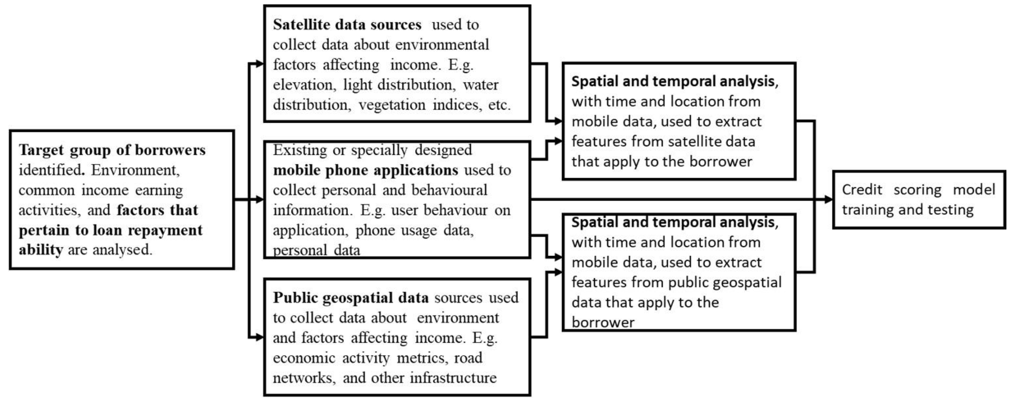
3. Proposed Approach
4. Methods
4.1. Multiple Logistic Regression
4.2. Support Vector Machines (SVM)
4.3. Artificial Neural Networks (ANNs)
4.4. Ensemble Methods
4.5. Model-Evaluation Methods
5. Empirical Evaluation
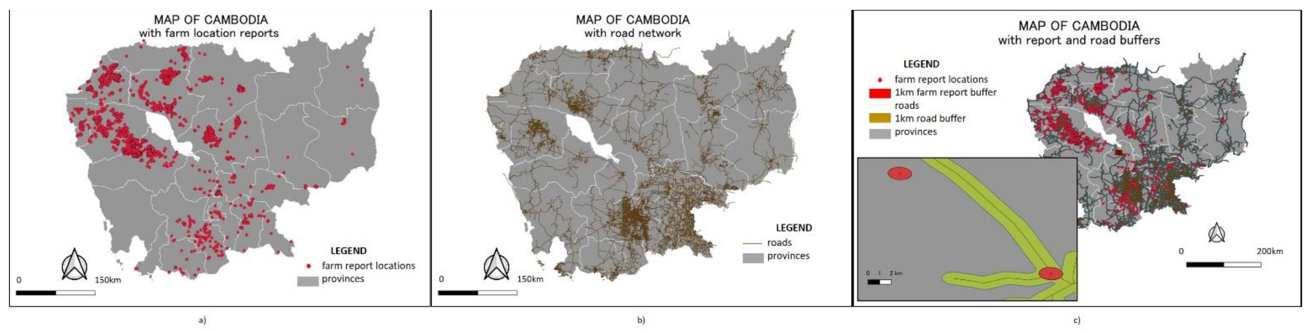
5.1. Study Area
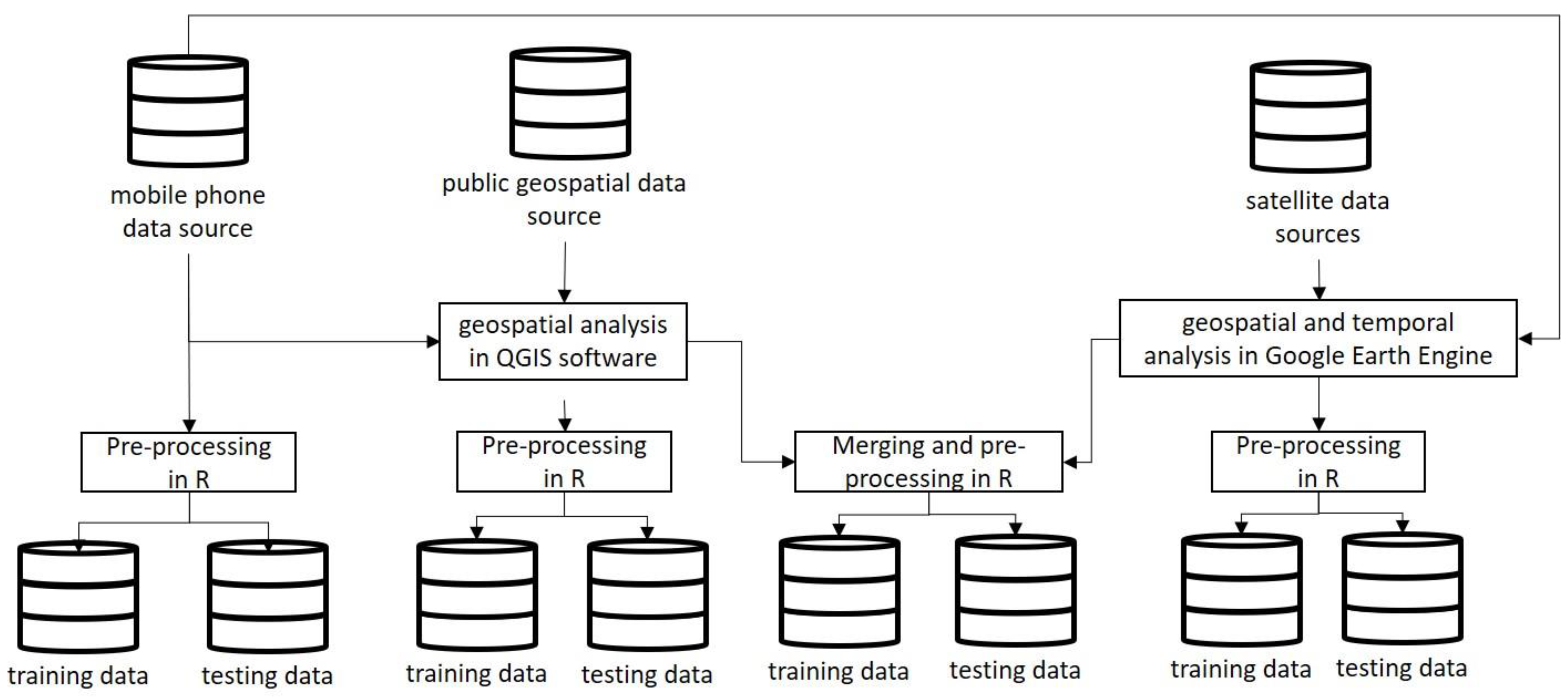
5.2. Data Collection and Preparation
5.2.1. Credit Data
5.2.2. Mobile-Phone Data
5.2.3. Public Geospatial Data
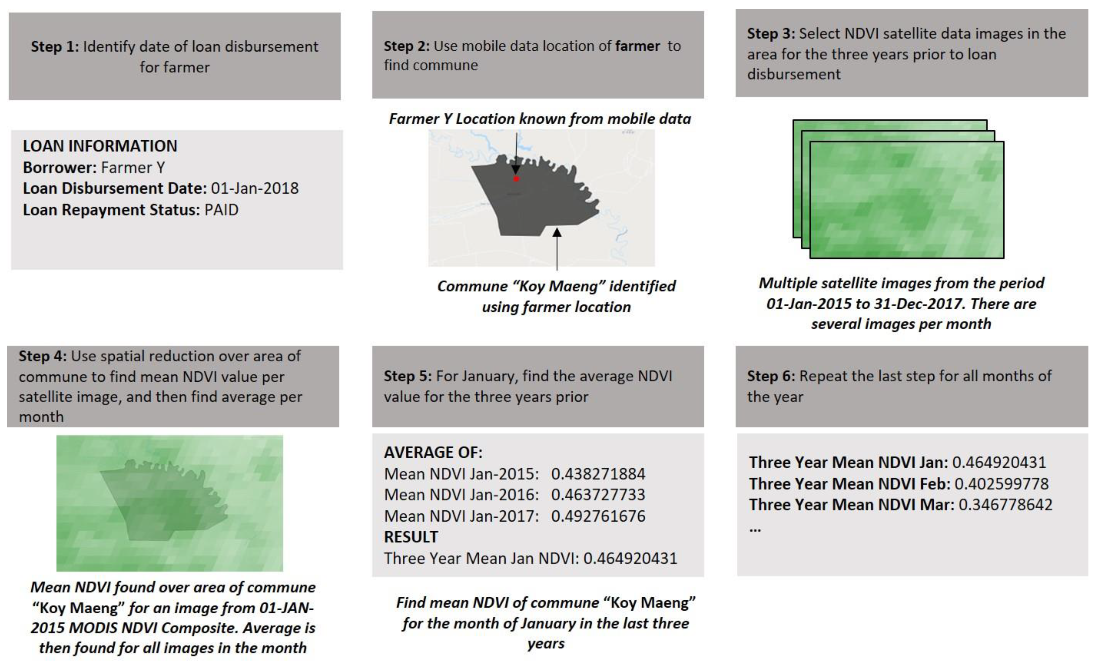
5.2.4. Satellite Data
6. Analysis
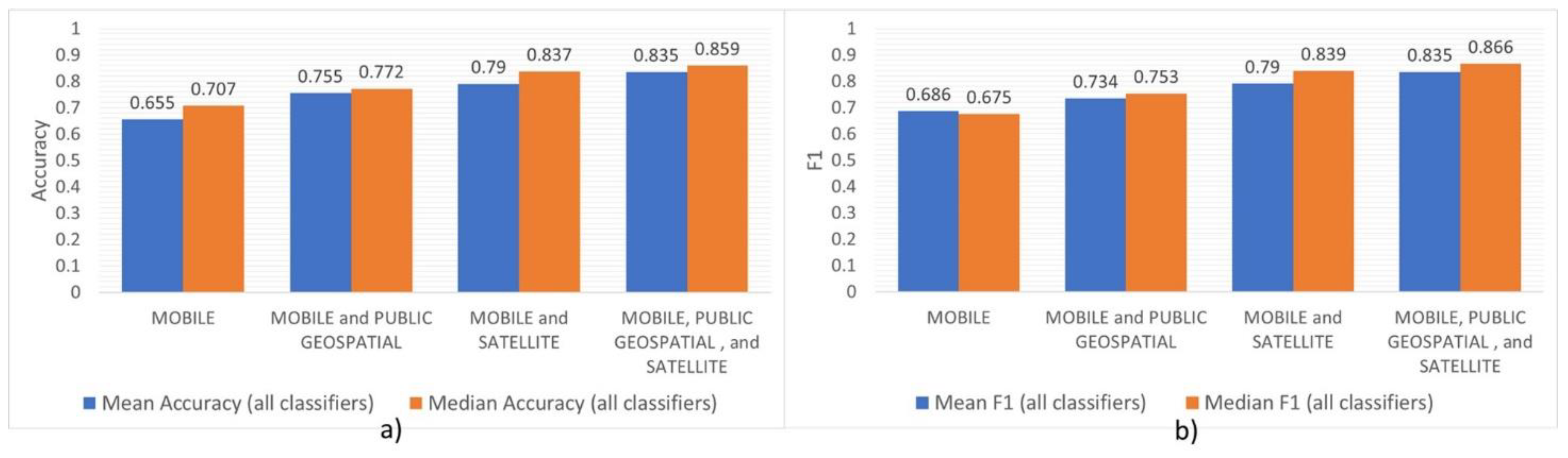
7. Results
8. Discussion
8.1. Data Combination
8.2. Alternative Data
8.3. Classification Methods
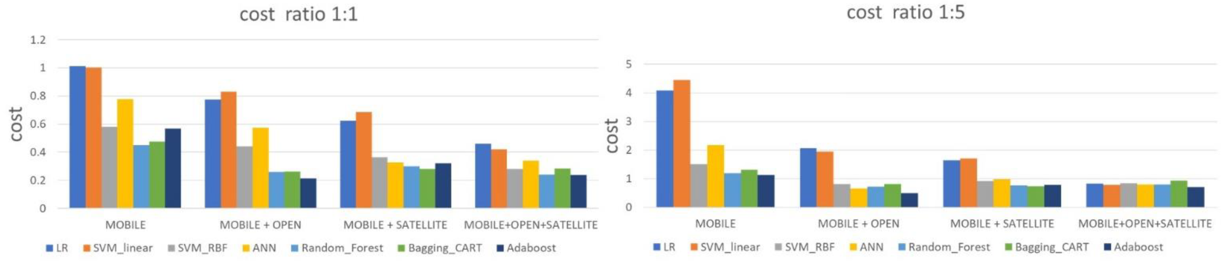
8.4. Cost of Misclassification
8.5. General Implementation
9. Conclusions
10. Future Work
Author Contributions
Funding
Institutional Review Board Statement
Informed Consent Statement
Data Availability Statement
Acknowledgments
Conflicts of Interest
Appendix A

| Classifier | Mobile-Phone Data | Mobile and Public Geospatial Data | Mobile and Satellite Data | Mobile, Satellite, and Public Geospatial Data |
|---|---|---|---|---|
| SVM—linear | cost = 1 | cost = 1 | cost = 1 | cost = 1 |
| SVM—RBF | sigma = 8.915, cost = 64 | sigma = 0.134, cost = 32 | sigma = 0.343, cost = 16 | sigma = 0.074, cost = 128 |
| ANN | size of hidden layer = 5, decay = 0.0001 | size of hidden layer = 5, decay = 0.1 | size of hidden layer = 5, decay = 0.0001 | size of hidden layer = 5, decay = 0.1 |
| Random Forest | Number of variables randomly collected to be sampled at each split time (mtry) = 5 | Number of variables randomly collected to be sampled at each split time (mtry) = 9 | Number of variables randomly collected to be sampled at each split time (mtry) = 3 | Number of variables randomly collected to be sampled at each split time (mtry) = 3 |
| AdaBoost | method = AdaBoost.M1, iterations = 100 | method = AdaBoost.M1, iterations = 50 | method = AdaBoost.M1, iterations = 50 | method = AdaBoost.M1, iterations = 50 |
References
- Demirgüç-Kunt, A.; Klapper, L.; Singer, D.; Ansar, S.; Hess, J. The Global Findex Database; World Bank Group: Washington, DC, USA, 2017. [Google Scholar]
- Grandolini, M.G. Five Challenges Prevent Financial Access for People in Developing Countries. World Bank, 15 10 2015. Available online: https://blogs.worldbank.org/voices/five-challenges-prevent-financial-access-people-developing-countries (accessed on 15 August 2017).
- McEvoy, M.J. Enabling Financial Inclusion through Alternative Data; Mastercard Advisors: New York, NY, USA, 2014. [Google Scholar]
- Turner, M.A.; Walker, P.D.; Chaudhuri, S.; Varghese, R. New Pathway to Financial Inclusion; Policy & Economic Research Council (PERC): Melbourne, Australia, 2012. [Google Scholar]
- Global and Regional ICT Estimates; International Telecommunications Union: Geneva, Switzerland, 2018.
- Costa, A.; Deb, A.; Kubzansky, M. Big data, small credit: The digital revolution and its impact on emerging market consumers. Innov. Technol. Gov. Glob. 2015, 10, 49–80. [Google Scholar] [CrossRef]
- Donaldson, D.; Storeygard, A. The view from above: Applications of satellite data in economics. J. Econ. Perspect. 2016, 30, 171–198. [Google Scholar] [CrossRef]
- QGIS Development Team. QGIS Geographic Information System. Open Source Geospatial Foundation Project. Available online: http://qgis.osgeo.org (accessed on 5 May 2018).
- Gorelick, N.; Hancher, M.; Dixon, M.; Ilyushchenko, S.; Thau, D.; Moore, R. Google earth engine: Planetary-scale geospatial analysis for everyone. Remote Sens. Environ. 2017, 202, 18–27. [Google Scholar] [CrossRef]
- Thomas, L.C.; Edelman, B.D.; Crook, N.J. Credit Scoring and Its Applications; Society for Applied and Industrial Mathematics: Philadelphia, PA, USA, 2002. [Google Scholar]
- Lessmann, S.; Baesens, B.; Seow, H.-V.; Thomas, L.C. Benchmarking state-of-the-art classification algorithms for credit scoring: An update of research. Eur. J. Oper. Res. 2015, 247, 124–136. [Google Scholar] [CrossRef]
- Papouskova, M.; Hajek, P. Two-stage consumer credit risk modelling using heterogeneous ensemble learning. Decis. Support Syst. 2019, 118, 33–45. [Google Scholar] [CrossRef]
- Harris, T. Credit scoring using the clustered support vector machine. Expert Syst. Appl. 2015, 42, 741–750. [Google Scholar] [CrossRef]
- Verbraken, T.; Bravo, C.; Weber, R.; Baesens, B. Development and application of consumer credit scoring models using profit-based classification measures. Eur. J. Oper. Res. 2014, 238, 505–513. [Google Scholar] [CrossRef]
- Serrano-Cinca, C.; Gutiérrez-Nieto, B. The use of profit scoring as an alternative to credit scoring systems in peer-to-peer (P2P) lending. Decis. Support Syst. 2016, 89, 113–122. [Google Scholar] [CrossRef]
- Robinson, D.; Yu, H. Knowing the Score: New Data, Underwriting, and Marketing in the Consumer Credit Marketplace (October 2014). Available online: https://www.upturn.org/static/files/Knowing_the_Score_Oct_2014_v1_1.pdf (accessed on 2 January 2021).
- Bjorkegren, D.; Grissen, D. Behavior revealed in mobile phone usage predicts loan repayment. SSRN Electron. J. 2018. [Google Scholar] [CrossRef]
- Óskarsdóttir, M.; Bravo, C.; Sarraute, C.; Vanthienen, J.; Baesens, B. The value of big data for credit scoring: Enhancing financial inclusion using mobile phone data and social network analytics. Appl. Soft Comput. 2019, 74, 26–39. [Google Scholar] [CrossRef]
- Simumba, N.; Okami, S.; Kodaka, A.; Kohtake, N. Alternative scoring factors using non-financial data for credit decisions in agricultural microfinance. In Proceedings of the IEEE International Symposium on Systems Engineering, Rome, Italy, 1–3 October 2018. [Google Scholar]
- Ntwiga, B.D.; Weke, P. Credit scoring for M-Shwari using hidden markov model. Eur. Sci. J. 2013, 12, 15. [Google Scholar]
- Lohokare, J.; Dani, R.; Sontakke, S. Automated data collection for credit score calculation based on financial transactions and social media. In Proceedings of the 2017 International Conference on Emerging Trends & Innovation in ICT (ICEI), Yashada, Pune, 3–5 February 2017; pp. 134–138. [Google Scholar]
- Li, Y.; Wang, X.; Djehiche, B.; Hu, X. Credit scoring by incorporating dynamic networked information. Eur. J. Oper. Res. 2020, 286, 1103–1112. [Google Scholar] [CrossRef]
- Djeundje, V.B.; Crook, J.; Calabrese, R.; Hamid, M. Enhancing credit scoring with alternative data. Expert Syst. Appl. 2021, 163, 113766. [Google Scholar] [CrossRef]
- Blanco, A.; Pino-Mejías, R.; Lara, J.; Rayo, S. Credit scoring models for the microfinance industry using neural networks: Evidence from Peru. Expert Syst. Appl. 2013, 40, 356–364. [Google Scholar] [CrossRef]
- Djeundje, V.B.; Crook, J. Incorporating heterogeneity and macroeconomic variables into multi-state delinquency models for credit cards. Eur. J. Oper. Res. 2018, 2, 697–709. [Google Scholar] [CrossRef]
- Fernandes, G.B.; Artes, R. Spatial dependence in credit risk and its improvement in credit scoring. Eur. J. Oper. Res. 2016, 249, 517–524. [Google Scholar] [CrossRef]
- Sowers, D.C.; Durand, D. Risk elements in consumer instalment financing. J. Mark. 1942, 6, 407. [Google Scholar] [CrossRef]
- Ben-Hur, A.W.J. A.W.J. A User’s Guide to Support Vector Machines. In Data Mining Techniques for the Life Sciences; Humana Press: Totowa, NJ, USA, 2010; pp. 223–239. [Google Scholar]
- Haltuf, M. Support Vector Machines for Credit Scoring; University of Economics in Prague, Faculty of Finance: Prague, Czech Republic, 2014. [Google Scholar]
- Zheng, R.Y. Neural Networks. In Data Mining Techniques for the Life Sciences; Human Press: Totowa, NJ, USA, 2010; pp. 197–222. [Google Scholar]
- Breiman, L. Bagging predictors. Machin. Learn. 1996, 24, 123–140. [Google Scholar] [CrossRef]
- Schapire, R. The strength of weak learnability. Mach. Learn. 1989, 5, 197–227. [Google Scholar] [CrossRef]
- Freund, Y.; Schapire, R.E. Experiments with a new boosting algorithm. In Proceedings of the Machine Learning: Thirteenth International Conference, Bari, Italy, 3–6 July 1996; pp. 148–156. [Google Scholar]
- Fawcett, T. An introduction to ROC analysis. Pattern Recognit. Lett. 2006, 27, 861–874. [Google Scholar] [CrossRef]
- Economic Research and Regional Cooperation Department. Basic Statistics 2017; Asian Development Bank (ADB): Manila, Philippines, 2017. [Google Scholar]
- National Institute of Statistics, Ministry of Planning. Census of Agriculture in Cambodia 2013; Ministry of Agriculture, Forestry and Fisheries: Phnom Penh, Cambodia, 2015. [Google Scholar]
- Food and Agriculture Organisation of the United Nations. FAO Statistical Pocketbook World Food and Agriculture; Food and Agriculture Organisation of the United Nations: Rome, Italy, 2015. [Google Scholar]
- World Bank. Global Financial Inclusion Statistics; World Bank Group: Washington, DC, USA, 2014. [Google Scholar]
- East-West Management Institute. Open Development Cambodia. Available online: https://opendevelopmentcambodia.net/maps/ (accessed on 10 November 2018).
- Skakun, S.; Kussul, N.; Shelestov, A.; Kussul, O. The use of satellite data for agriculture drought risk quantification in Ukraine. Geomat. Nat. Hazards Risk 2015, 7, 901–917. [Google Scholar] [CrossRef]
- Jarvis, A.; Reuter, H.I.; Nelson, A.; Guevara, E. Hole-filled SRTM for the globe Version 4. Available from the CGIAR-CSI SRTM 90 m Database. Available online: http://srtm.csi.cgiar.org (accessed on 24 November 2019).
- Schaaf, C.W.Z. MCD43A4 MODIS/Terra+Aqua BRDF/Albedo Nadir BRDF Adjusted Ref Daily L3 Global-500 m V006 [Data set]. NASA EOSDIS Land Processes DAAC. Available online: https://lpdaac.usgs.gov/products/mcd43a4v006/ (accessed on 24 November 2019).
- Wan, Z.H.S.H.G. MOD11A1 MODIS/Terra Land Surface Temperature/Emissivity Daily L3 Global 1km SIN Grid V006 [Data set]. NASA EOSDIS Land Processes DAAC. Available online: https://lpdaac.usgs.gov/products/mod11a1v006/ (accessed on 24 November 2019).
- Vermote, E.W.R. MOD09GA MODIS/Terra Surface Reflectance Daily L2G Global 1 km and 500 m SIN Grid V006 [Data set]. NASA EOSDIS Land Processes DAAC. Available online: https://lpdaac.usgs.gov/products/mod09gav006/ (accessed on 24 November 2019).
- Demsar, J. Statistical comparisons of classifiers over multiple data sets. J. Mach. Learn. Res. 2006, 7, 1–30. [Google Scholar]
- Nemenyi, P.B. Distribution-Free Multiple Comparisons; Princeton University: Princeton, NJ, USA, 1963. [Google Scholar]


| Data Source | Variables | Type | Importance |
|---|---|---|---|
| Mobile-phone data | Has uploaded a photo of the family | Nominal | 0.518 |
| Has uploaded a photo of the house | Nominal | 0.508 | |
| Has uploaded a photo of the land document | Nominal | 0.514 | |
| Has uploaded a photo of the ID card | Nominal | 0.508 | |
| Number of farms registered | Numeric | 0.614 | |
| Satellite data | Mean July temperature | Numeric | 0.734 |
| Mean November NDVI | Numeric | 0.697 | |
| Mean September NDWI | Numeric | 0.778 | |
| Farm elevation | Numeric | 0.661 | |
| Farm slope | Numeric | 0.603 | |
| Public geospatial data | Farm is within 1 km of a canal | Nominal | 0.642 |
| Farm is within 2 km of a canal | Nominal | 0.629 | |
| Farm is within 1 km of a road | Nominal | 0.569 | |
| Farm is within 2 km of a road | Nominal | 0.568 | |
| Farm is within 5 km of a river | Nominal | 0.558 |
| Classifier | Mobile-Phone Data | Mobile and Public Geospatial Data | Mobile and Satellite Data | Mobile, Satellite, and Public Geospatial Data |
|---|---|---|---|---|
| LR | 0.582 | 0.679 | 0.814 | 0.824 |
| SVM—linear | 0.484 | 0.637 | 0.800 | 0.821 |
| SVM—RBF | 0.725 | 0.846 | 0.874 | 0.902 |
| ANN | 0.688 | 0.805 | 0.839 | 0.861 |
| Random Forest | 0.814 | 0.922 | 0.93 | 0.938 |
| Bagging CART | 0.863 | 0.917 | 0.917 | 0.919 |
| AdaBoost | 0.687 | 0.771 | 0.831 | 0.828 |
| Classifier | Mobile-Phone Data | Mobile and Public Geospatial Data | Mobile and Satellite Data | Mobile, Satellite, and Public Geospatial Data |
|---|---|---|---|---|
| LR | 0.511 | 0.609 | 0.685 | 0.761 |
| SVM—linear | 0.522 | 0.577 | 0.653 | 0.783 |
| SVM—RBF | 0.707 | 0.772 | 0.816 | 0.859 |
| ANN | 0.609 | 0.696 | 0.837 | 0.827 |
| Random Forest | 0.772 | 0.870 | 0.848 | 0.881 |
| Bagging CART | 0.761 | 0.870 | 0.859 | 0.859 |
| AdaBoost | 0.707 | 0.892 | 0.837 | 0.881 |
| Classifier | Mobile-Phone Data | Mobile and Public Geospatial Data | Mobile and Satellite Data | Mobile, Satellite, and Public Geospatial Data |
|---|---|---|---|---|
| LR | 0.756 | 0.552 | 0.633 | 0.633 |
| SVM—linear | 0.858 | 0.449 | 0.572 | 0.674 |
| SVM—RBF | 0.654 | 0.654 | 0.776 | 0.858 |
| ANN | 0.572 | 0.449 | 0.837 | 0.776 |
| Random Forest | 0.735 | 0.858 | 0.817 | 0.898 |
| Bagging CART | 0.735 | 0.878 | 0.837 | 0.878 |
| AdaBoost | 0.572 | 0.858 | 0.796 | 0.878 |
| Classifier | Mobile-Phone Data | Mobile and Public Geospatial Data | Mobile and Satellite Data | Mobile, Satellite, and Public Geospatial Data |
|---|---|---|---|---|
| LR | 0.233 | 0.675 | 0.745 | 0.907 |
| SVM—linear | 0.140 | 0.721 | 0.745 | 0.907 |
| SVM—RBF | 0.768 | 0.907 | 0.861 | 0.861 |
| ANN | 0.652 | 0.977 | 0.838 | 0.884 |
| Random Forest | 0.814 | 0.884 | 0.884 | 0.861 |
| Bagging CART | 0.791 | 0.861 | 0.884 | 0.838 |
| AdaBoost | 0.861 | 0.931 | 0.884 | 0.884 |
| Classifier | Mobile-Phone Data | Mobile and Public Geospatial Data | Mobile and Satellite Data | Mobile, Satellite, and Public Geospatial Data |
|---|---|---|---|---|
| LR | 0.622 | 0.600 | 0.682 | 0.739 |
| SVM—linear | 0.657 | 0.531 | 0.637 | 0.768 |
| SVM—RBF | 0.704 | 0.753 | 0.818 | 0.866 |
| ANN | 0.609 | 0.612 | 0.846 | 0.827 |
| Random Forest | 0.775 | 0.875 | 0.852 | 0.889 |
| Bagging CART | 0.766 | 0.878 | 0.864 | 0.869 |
| AdaBoost | 0.675 | 0.894 | 0.839 | 0.887 |
| Classifier | Mobile-Phone Data | Mobile and Public Geospatial Data | Mobile and Satellite Data | Mobile, Satellite, and Public Geospatial Data |
|---|---|---|---|---|
| LR | 0.927 | 1.026 | 1.516 | 1.180 |
| SVM—linear | 1.437 | 1.561 | 2.218 | 2.075 |
| SVM—RBF | 15.081 | 15.082 | 18.172 | 16.090 |
| ANN | 10.201 | 11.652 | 12.185 | 12.563 |
| Random Forest | 12.409 | 27.090 | 26.879 | 44.580 |
| Bagging CART | 4.470 | 5.162 | 5.373 | 6.069 |
| AdaBoost | 2.404 | 3.426 | 3.623 | 4.768 |
| Data | Average Ranks | Nemenyi Post Hoc Test p-Values | ||
|---|---|---|---|---|
| Mobile-Phone Data | Mobile and Public Geospatial Data | Mobile and Satellite Data | ||
| Mobile-phone data | 4 | |||
| Mobile and public geospatial data | 2.286 | 0.062 | ||
| Mobile and satellite data | 2.214 | 0.048 | 1 | |
| Mobile, satellite, and public geospatial data | 1.500 | 0.002 | 0.666 | 0.729 |
| Friedman statistic | 14.391 | |||
| Friedman p value | 0.002 | |||
Publisher’s Note: MDPI stays neutral with regard to jurisdictional claims in published maps and institutional affiliations. |
© 2021 by the authors. Licensee MDPI, Basel, Switzerland. This article is an open access article distributed under the terms and conditions of the Creative Commons Attribution (CC BY) license (https://creativecommons.org/licenses/by/4.0/).
Share and Cite
Simumba, N.; Okami, S.; Kodaka, A.; Kohtake, N. Spatiotemporal Integration of Mobile, Satellite, and Public Geospatial Data for Enhanced Credit Scoring. Symmetry 2021, 13, 575. https://doi.org/10.3390/sym13040575
Simumba N, Okami S, Kodaka A, Kohtake N. Spatiotemporal Integration of Mobile, Satellite, and Public Geospatial Data for Enhanced Credit Scoring. Symmetry. 2021; 13(4):575. https://doi.org/10.3390/sym13040575
Chicago/Turabian StyleSimumba, Naomi, Suguru Okami, Akira Kodaka, and Naohiko Kohtake. 2021. "Spatiotemporal Integration of Mobile, Satellite, and Public Geospatial Data for Enhanced Credit Scoring" Symmetry 13, no. 4: 575. https://doi.org/10.3390/sym13040575
APA StyleSimumba, N., Okami, S., Kodaka, A., & Kohtake, N. (2021). Spatiotemporal Integration of Mobile, Satellite, and Public Geospatial Data for Enhanced Credit Scoring. Symmetry, 13(4), 575. https://doi.org/10.3390/sym13040575