A Time-Variant Reliability Analysis Method Based on the Stochastic Process Discretization under Random and Interval Variables

Abstract

In practical engineering, it is a cost-consuming problem to consider the time-variant reliability of both random variables and interval variables, which usually requires a lot of calculation. Therefore, a time-variant reliability analysis approach with hybrid uncertain variables is proposed in this paper. In the design period, the stochastic process is discretized into random variables. Simultaneously, the original random variables and the discrete random variables are converted into independent normal variables, and the interval variables are changed into standard variables. Then it is transformed into a hybrid reliability problem of static series system. At different times, the limited state functions are linearized at the most probable point (MPP) and at the most unfavorable point (MUP). The transformed static system reliability problem with hybrid uncertain variables can be solved effectively by introducing random variables. To solve the double-loop nested optimization in the hybrid reliability calculation, an effective iterative method is proposed. Two numerical examples and an engineering example demonstrate the validity of the present approach.

1. Introduction

Due to structural material performance degradation, changing working environment, time-variant load effects, etc., the reliability of the structure exhibits time-variant properties [1,2,3,4,5,6]. Over the past decades, different time-variant reliability analysis methods have been developed including first-passage approaches, numerical simulation approaches, extreme value approaches and quasi-static approaches. The first-passage methods based on out-crossing events [7] have been developed. The representative methods are the PHI2 method [8], improved PHI2 method [9] and joint out-crossing rate method [10,11]. Although many first-passage methods [10,12,13] aimed at accuracy and efficiency have been developed for two decades, it is generally hard to achieve the first-time out-crossing rate due to complicated mathematical characteristics. Different numerical simulation methods have been developed including Monte Carlo methods [14] and their improved versions, namely important sampling methods [15,16] and subset methods [17,18,19]. Although the numerical simulation method is accurate, it demands huge computational cost. The extremum method [20,21,22,23] mainly focuses on the worst scenario over the time scale, in which surrogate model or probability distribution are used to describe the uncertainty of response extremum for time-variant problem. In some cases, the extreme value distribution may be subject to multi-modal or highly non-linear distribution, and the realistic application of the extreme value method is hindered. Recently, the quasi-static methods have been developed to improve efficiency, such as the stochastic process discretization approach [24] and the envelope method [25]. These methods translate the estimation of time-dependent failure probability into the estimation of time-independent failure probability. The stochastic process discretization approach is considered in this study. Gong and Zhao [26] proposed a structural reliability analysis method considering the change of resistance. Jiang et al. [24] developed a method for solving time-variant reliability based on process discretization (TRPD). The idea is to discretize the stochastic process and obtain several random variables, so that the time-variant reliability problem can be transformed into the time-invariant reliability problem, thus avoiding the solution of the crossover rate. Then the method is extended to the reliability analysis of time-variant systems [27]. Jiang et al. [28] proposed the improved TRPD, in which time invariant reliability analysis is only performed at the component level, and no new random variables are needed. It makes the solving process more concise and clearer, and effectively saves the calculation cost. Cazuguel et al. [29] transformed the time-variant reliability model into the static reliability model by expressing the Gaussian process as multiple independent standard normal distributions. Gong and Frangopol [30] discretized the time interval considered into many uniformly distributed time moments. At each moment, the first-order reliability analysis method (FORM) is used to calculate the instantaneous reliability, and finally the time-variant reliability is calculated by using the multivariate normal distribution function.

The above stochastic process discretization approach only deals with random variables of probability distribution. However, for short enough sample data in engineering, the precise distribution of uncertain parameters is difficult to obtain, and the range of uncertain parameters is often easy to achieve. Interval is suitable to describe such uncertain variables [31,32,33,34,35]. Although the time-variant reliability method based on the discrete stochastic process method has made some progress, the time-variant reliability method based on random parameters and interval parameters is still in its infancy [2], and there are still some technical problems to be solved. First, general forms of time-variant reliability analysis issues with mixed variables are still lacking. Special cases of mixed time-variant reliability have been studied by Shi [36], in which the correlation at each moment has not been considered. Second, the reliability analysis is a multi-level nested optimization problem at each moment, and efficiency is difficult to be guaranteed. Therefore, it is an important engineering significance to study effective time-variant reliability methods.

A reliability analysis method of the time-variant method with stochastic process discretization is presented in this paper to tackle the above issue. The remaining structure of this paper is organized as follows. Section 2 represents the problem of general time-variant reliability. A general time-variant reliability model with random variables and interval variables and its effective solution algorithm are provided in Section 3. An analysis of the examples is given in Section 4. Section 5 is the conclusion.

2. Problem of General Time-Variant Reliability Model

Time-variant reliability of structures refers to the possibility of completing predetermined functions within a specified time and under specified conditions for structures subjected to dynamic uncertainties. For a specific structure whose limit-state function is $g(X(t),Y,t)$, the probability of structural reliability within the time period [0, T] can be defined as:

$$P_s(T)=\mathrm{Pr}\mathrm{ob}\left\{\forall t\in \left[0,T\right]|g(X(t),Y,t)>0\right\}$$

(1)

where Prob stands for probability operation, t is the time, T is the design lifetime, $X(t)=\left[X_1(t),X_2(t),\dots ,X_n(t)\right]$ is the n-dimensional stochastic process vector, and $Y=\left[Y_1,Y_2,\dots ,Y_h\right]$ is the h-dimensional random vector. The out-crossing rate method is the most commonly used method to solve time-variant reliability problems. But sometimes it is difficult to calculate the crossing rate accurately and effectively.

The time-variant reliability analysis method based on stochastic process discretization avoids the calculation of out-crossing rate and simplifies the solving process of time-variant reliability. According to the method in literature [26,27], the design lifetime T is discretized into m equal periods with each time step size $\nabla t=\frac{T}{m}$. According to the reliability calculation theory of series system, Equation (1) can be changed into:

$$P_s(T)=\left\{{\displaystyle \underset{i=1}{\overset{m}{\cap }}\left[g(X_i,Y,t_i)>0,t_i=(i-\frac{1}{2})\Delta t,\Delta t=\frac{T}{m}\right]}\right\}$$

(2)

where $X_i=[X_1(t_i),X_2(t_i),\dots ,X_n(t_i{)]}^T=(X_{i,1},X_{i,2},\dots ,X_{i,n}),i=1,2,\dots ,\mathrm{m},$ $(X_{i,1},X_{i,2},\dots ,X_{i,n}),i=1,2,\dots ,m,$ and $(X_1^T,X_2^T,\dots ,X_m^T)$ is $m\times n$ dimensional random variable obtained by the discrete process X(t). Obviously, Equation (2) is a time-variant reliability problem with only random variables. If all random variables can provide accurate probability distribution, the reliability calculation can be carried out by using the conventional probability model.

3. Problem of General Time-Variant Reliability Model with Random and Interval Variables

Due to the lack of accurate probability distribution of uncertain parameters in the time-variant reliability problem, the interval ranges of uncertain parameters are relatively easy to be given. Therefore, a time-variant reliability analysis model for random variables and interval variables is constructed. The limit-state function of hybrid uncertain variables can be formulated as

$$P_s(T)=\mathrm{Pr}\mathrm{ob}\left\{\forall t\in \left[0,T\right]|g(X(t),Y,q,t)>0\right\}$$

(3)

where $q=\left[q_1,q_2,\dots ,q_l\right]$ is the l-dimensional interval vector. The corresponding interval vector can be defined as

$$q^I\in [q^L,q^R],q_i\in [q_i^L,q_i^R],i=1,2,\dots ,l$$

(4)

where superscript I, L and R represent interval, upper and lower ranges of interval, respectively.

$$P_s(T)=\left\{{\displaystyle \underset{i=1}{\overset{m}{\cap }}\left[g(X_i,Y,q,t_i)>0,t_i=(i-\frac{1}{2})\Delta t,\Delta t=\frac{T}{m}\right]}\right\}$$

(5)

3.1. Normalization of Random Variables

In the process of time-variant reliability analysis, the Nataf transformation [37] is first adopted to transform the random variable (X, Y) at time $t_i$ into the standard normal space:

$$\left[U_i;{\mathsf{\rho }}_U\right]=Nataf\left[X_i;{\mathsf{\rho }}_X\right]$$

(6)

$$(V;{\mathsf{\rho }}_V)=Nataf(Y;{\mathsf{\rho }}_Y)$$

(7)

where Nataf(·) represents the Nataf transformation. ${\mathsf{\rho }}_X$ and ${\mathsf{\rho }}_Y$ are the correlation coefficient matrices of the random variable $X_i$ and Y, respectively. ${\mathsf{\rho }}_U$ and ${\mathsf{\rho }}_V$ are the correlation coefficient matrices of the standard normal variable U and V, respectively.

Let the covariance of the random variable $U=(U_1,U_2,\dots ,U_m{)}^T$ be ${\mathsf{\rho }}_U=[{\rho }_{U_i}{\rho }_{U_j}{]}_{m\times m}$, where $i=1,2,\dots ,m$, $j=1,2,\dots ,m$. The diagonal element is the variance ${\sigma }_{U_i}^2$ of the variable $U_i$, the non-diagonal element is the covariance $C_U=\mathrm{Cov}(U_i,U_j)$ of the variable $U_i$ and $U_j$, and the $C_U=\mathrm{Cov}(U_i,U_j)$ is a symmetric positive definite matrix of order n, which can be expressed as follows:

$${\mathrm{C}}_U={\rho }_U=\left[\begin{array}{l}\begin{array}{cccc}\mathrm{Cov}(U_1,U_1)& \mathrm{Cov}(U_2,U_1)& \cdots & \mathrm{Cov}(U_m,U_1)\end{array}\\ \begin{array}{cccc}\mathrm{Cov}(U_1,U_2)& \mathrm{Cov}(U_2,U_2)& \cdots & \mathrm{Cov}(U_m,U_2)\end{array}\\ \begin{array}{ccc}\begin{array}{ccc}\begin{array}{ccc}\begin{array}{cccc}\begin{array}{cccc}\begin{array}{cc}& \end{array}& ⋮& & \end{array}& & & ⋮\end{array}& & \end{array}& & \end{array}& & ⋮\end{array}\\ \begin{array}{cccc}\mathrm{Cov}(U_1,U_m)& \mathrm{Cov}(U_2,U_m)& \cdots & \mathrm{Cov}(U_m,U_m)\end{array}\end{array}\right]$$

(8)

The above m-order symmetric positive definite matrix ${\mathrm{C}}_U$ has m linearly independent eigenvectors ${\alpha }_1,{\alpha }_2,\dots ,{\alpha }_m$. Let the linear transformation matrix be $A=[{\alpha }_1,{\alpha }_2,\dots ,{\alpha }_m],$ then $A^{-1}{C}_{U}A=\Lambda$. $\Lambda$ denotes an N-order diagonal matrix whose diagonal element is the eigenvalue ${\lambda }_i,i=1,\dots ,m$ of the orthogonal matrix $A$. Relevant normal random variable U can be changed into independent normal random variable P by the method of orthogonal transformation [37].

$$U=AP$$

(9)

The random vector $U$ is changed into a linearly independent random vector $P$. It is known from the matrix theory that $A^{-1}=A^T$, and Equation (9) can be written as

$$P=A^{T}U$$

(10)

Superscript T indicates the transpose of the matrix.

Through the orthogonal transformation of Equation (10), the covariance matrix $C_P$ can be transformed into the following form

$$C_P=\mathrm{Cov}(P_i,P_j)=\mathrm{Cov}(P,P^T)=\mathrm{Cov}(A^{T}U,U^{T}A)=A^T\mathrm{Cov}(U,U^T)A=A^T{\mathrm{C}}_{U}A$$

(11)

Similarly, the correlated random variable V can be transformed into the uncorrelated random variable Q by orthogonal transformation.

$$Q=B^{T}V$$

(12)

where B is a linear transformation matrix.

3.2. Normalization of Interval Variables

The interval variables q can be expressed as

$$q_i\in q_i^I=[q_i^L,q_i^R]=[q_i^C-q_i^W,q_i^C+q_i^W],i=1,2,\dots ,l$$

(13)

where superscript C and W are the midpoint and radius of the interval, respectively.

$$q_i^C=\frac{q_i^L+q_i^R}{2},q_i^w=\frac{q_i^R-q_i^L}{2},i=1,2,\dots ,l$$

(14)

The interval is normalized

$$q_i=q_i^C+{\delta }_i{q}_i^R,i=1,2,\dots ,l$$

(15)

${\delta }_i(i=1,2,\dots ,l)$ is a standardized interval variable. The uncertainty domain $C_{\delta }=\left\{\delta |{\delta }_i\in \left[-1,1\right],i=1,2,\dots ,l\right\}$ becomes a standard multi-dimensional cube, and the center coincides with the origin.

3.3. Solution of Time-Invariant Reliability Problem

After the normalized transformation of the above hybrid uncertain variables, at the time $t_i$, the limit-state function $g(X_i,Y,q,t_i)$ in the original uncertainty variable space is mapped to its standardized form $G(P_i,Q,\delta ,t_i)$.

Because of involving random variables and interval variables, the limit-state equation of a structure $G(P_i,Q,\delta ,t_i)=0$ forms a critical region of a strip. Thus, the entire standard space is divided into three parts: the safety zone, the critical zone and the failure zone. Schematic diagram for two random variables (P, Q) in two-dimensional standard space is shown in Figure 1. Therefore, we define the reliability of the structure in the mixed model: the probability that the structure can perform at least the predetermined function of the structure for any possible implementation of the interval parameter at a certain time. The mathematical formula is expressed as

$$P_h(T)=\left\{{\displaystyle \underset{i=1}{\overset{m}{\cap }}\left[\underset{\_}{G}=G(P_i,Q,\delta ,t_i)>0,t_i=(i-\frac{1}{2})\Delta t,\Delta t=\frac{T}{m}\right]}\right\}$$

(16)

where subscript h represents the mixed model, $\underset{\_}{G}=\underset{\delta }{\min }(P_i,Q,\delta ,t_i)$ and $\underset{\_}{G}=0$ represents the critical failure of the structure.

As an extension of the probabilistic reliability index, the mixed reliability index ${\beta }_h$ can be defined as the shortest distance from the origin to the most probable failure surface G(P, Q) = 0 in the standard space. Mathematically, it is the solution to the following optimization problem:

$$\begin{array}{l}{\beta }_h=\min \Vert {(P_i{}^T,Q_i{}^T)}^T\Vert \\ \mathrm{s}.\mathrm{t}.G(P_i,Q,{\delta }^{*},t_i)=0\end{array}$$

(17)

where ${\delta }^{*}$ is the most unfavorable point (MUP), which can be obtained through the following optimization:

$$\begin{array}{l}\underset{\delta }{\min } G(P_i,Q,\delta ,t_i)\\ \mathrm{s}.\mathrm{t}.{\delta }_i^T{\delta }_i^{}\le 1(i=1,2,\dots ,L)\end{array}$$

(18)

Equations (17) and (18) that define the hybrid reliability index are nested optimization problems. The most probable point (MPP) ${\overline{P}}_i,\overline{Q}$ is obtained in the outer loop optimization, while the most unfavorable point (MUP) ${\delta }^{*}$ is achieved in the inner loop optimization. The nested optimization problem in Equations (17) and (18) are solved by decoupling method. In turn, the inner and outer optimization problems can be solved according to the idea of the two-layer method.

In each iteration, MPP can be expressed as following:

$$\{\begin{array}{l}{\beta }^{k+1}=\frac{G(P_i^k,Q_i^k,{\delta }^{k+1})-{(\nabla G(P_i^k,Q_i^k,{\delta }^{k+1}))}^T{U}^k}{\Vert \nabla G(P_i^k,Q_i^k,{\delta }^{k+1})\Vert }\\ P_i^{k+1},Q_i^{k+1}=-{\beta }^{k+1}\frac{\nabla G(P_i^k,Q_i^k,{\delta }^{k+1})}{\Vert \nabla G(P_i^k,Q_i^k,{\delta }^{k+1})\Vert }\end{array}$$

(19)

In the above algorithm, ${\delta }^{k+1}$ is a fixed value. Once MPP points are obtained, interval variables ${\delta }^{k+1}$ can be obtained through the following optimization.

$$\begin{array}{l}\underset{\delta }{\min } G(P_i^{k+1},Q^{k+1},\delta ,t_i)\\ \mathrm{s}.\mathrm{t}.{\delta }_i^T{\delta }_i^{}\le 1(i=1,2,\dots ,L)\end{array}$$

(20)

In each iteration of MPP search, standardized interval variable $\delta$ is fixed. MPP algorithm updates the random variable, and optimizes the minimum limit-state function when random variable (P, Q) is fixed. The MUP ${\delta }_{}^{*}$ can be obtained by Equation (20).

For the convenience of analysis, the linear expansion of the static limit-state equations is carried out at the MPP and MUP ${\delta }_k^{*}$.

$$P_h(T)=\left\{{\displaystyle \underset{i=1}{\overset{m}{\cap }}\left[{\displaystyle \sum _{j=1}^n{\frac{\partial G_i}{\partial P_{i,j}}|}_{{\overline{P}}_{i,j}}(P_{i,j}-{\overline{P}}_{i,j})+{\displaystyle \sum _{k=1}^h{\frac{\partial G_i}{\partial Q_k}|}_{\overline{Q_k}}(Q_k-{\overline{Q}}_k)+{\displaystyle \sum _{l=1}^L{\frac{\partial G_i}{\partial {\delta }_l}|}_{\overline{{\delta }_l^{*}}}({\delta }_l-{\delta }_l^{*})}>0}}\right]}\right\}$$

(21)

Equation (21) can be converted to the following form:

$$P_h(T)=\left\{{\displaystyle \underset{i=1}{\overset{m}{\cap }}\left[{\displaystyle \sum _{j=1}^n{\frac{\partial G_i}{\partial P_{i,j}}|}_{{\overline{P}}_{i,j}}(-{\overline{P}}_{i,j})+{\displaystyle \sum _{k=1}^h{\frac{\partial G_i}{\partial Q_k}|}_{{\overline{Q}}_{i,k}}(Q_k-{\overline{Q}}_{i,k})+{\displaystyle \sum _{l=1}^L{\frac{\partial G_i}{\partial {\delta }_l}|}_{\overline{{\delta }_{i,l}^{*}}}({\delta }_l-{\delta }_{i,l}^{*})}>-{\displaystyle \sum _{j=1}^n{\frac{\partial G_i}{\partial P_{i,j}}|}_{{\overline{P}}_{i,j}}{P}_{i,j}}}}\right]}\right\}$$

(22)

A new random vector $\xi ={({\xi }_1,\dots ,{\xi }_m)}^T$ is introduced, which can be expressed as:

$${\xi }_i=-{\displaystyle \sum _{j=1}^n{\frac{\partial G_i}{\partial P_{i,j}}|}_{{\overline{P}}_{i,j}}{P}_{i,j},}i=1,2,\cdots ,m$$

(23)

Since $P_{i,j}$ represents a standard normal random variable, the random vector $\xi$ is the m-dimensional normal distribution. According to the properties of mean and covariance matrix of random vectors, we can define mean vector μ and covariance matrix C as:

$${({\mu }_{\xi })}_i=-{\displaystyle \sum _{j=1}^n{\frac{\partial G_i^{\prime }}{\partial P_{i,j}}|}_{{\overline{P}}_{i,j}}}{\mu }_{P_{i,j}}=0,i=1,2,\cdots ,m$$

(24)

$${(C_{\xi })}_{i,v}={\displaystyle \sum _{k=1}^n{\displaystyle \sum _{j=1}^n{\frac{\partial G_i^{\prime }}{\partial P_{i,j}}|}_{{\overline{P}}_{i,j}}}}{\frac{\partial G_v^{\prime }}{\partial P_{v,k}}|}_{{\overline{P}}_{v,k}}{\mathrm{C}}_P((i-1)n+j,(v-1)n+k),i,v=1,2,\dots ,m$$

(25)

where ${\mu }_{P_{i,j}}$ is the mean of ${\mu }_{P_{i,j}}$, and $(i-1)n+j$ and $(v-1)n+k$ in parentheses represent the numbers of rows and columns in the matrix, respectively. In order to understand the construction of ${\mathrm{C}}_P$, this paper gives the specific form of the matrix in four simple cases (See reference [24] for details). Integrating the m-dimensional normal distribution function, we change Equation (22) into the following expression:

$$\begin{array}{cc}{P}_h(T)=& {\displaystyle {\int }_0^{+\infty }{\displaystyle {\int }_0^{+\infty }\cdots }{\displaystyle {\int }_0^{+\infty }{\varphi }_m\left\{\left[{\displaystyle \sum _{j=1}^n{\frac{\partial G_i}{\partial P_{i,j}}|}_{\overline{P_{i,j}}}(-\overline{P_{i,j}})+{\displaystyle \sum _{k=1}^h{\frac{\partial G_i}{\partial Q_k}|}_{\overline{Q_{i,k}}}(Q_k-\overline{Q_{i,k}})+{\displaystyle \sum _{l=1}^L{\frac{\partial G_i}{\partial {\delta }_l}|}_{\overline{{\delta }_{i,l}^{*}}}({\delta }_l-{\delta }_{i,l}^{*})}}}\right],{\mu }_{\theta },{\mathrm{C}}_{\theta }\right\}}}\\ & \times f_Q(Q)\mathrm{d}Q\end{array}$$

(26)

${\varphi }_m$ is the probability distribution function of m-dimensional normal distribution. $f_Q(Q)$ denotes the joint probability density function of the random vector $Q$. Since Equation (26) is a multi-dimensional integration problem, the numerical solution requires a large amount of calculation. Therefore, this paper applies a new random variable $E$ and converts the formula Equation (26) into the following form.

$$\begin{array}{cc}{P}_h& (T)={\displaystyle \iint \cdots {\displaystyle \underset{\Omega }{\int }{f}_E(e)f_Q(Q)\mathrm{d}Q\mathrm{d}e}}\\ & =\mathrm{Pr}\mathrm{ob}\left\{F_E^{-1}\left\{{\varphi }_m\left\{\left[{\displaystyle \sum _{j=1}^n{\frac{\partial G_i}{\partial P_{i,j}}|}_{\overline{P_{i,j}}}(-\overline{P_{i,j}})+{\displaystyle \sum _{k=1}^h{\frac{\partial G_i}{\partial Q_k}|}_{\overline{Q_{i,k}}}(Q_k-\overline{Q_{i,k}})+{\displaystyle \sum _{l=1}^L{\frac{\partial G_i}{\partial {\delta }_l}|}_{\overline{{\delta }_{i,l}^{*}}}({\delta }_l-{\delta }_{i,l}^{*})}}}\right],{\mu }_{\theta },{\mathrm{C}}_{\theta }\right\}\right\}-E>0\right\}\end{array}$$

(27)

where $\Omega$ denotes the integral region, which can be expressed as:

$$\Omega =\left\{E,Q|E<F_E^{-1}\left\{{\varphi }_m\left\{\left[{\displaystyle \sum _{j=1}^n{\frac{\partial G_i}{\partial P_{i,j}}|}_{\overline{P_{i,j}}}(-\overline{P_{i,j}})+{\displaystyle \sum _{k=1}^h{\frac{\partial G_i}{\partial Q_k}|}_{\overline{Q_{i,k}}}(Q_k-\overline{Q_{i,k}})+{\displaystyle \sum _{l=1}^L{\frac{\partial G_i}{\partial {\delta }_l}|}_{\overline{{\delta }_{i,l}^{*}}}({\delta }_l-{\delta }_{i,l}^{*})}}}\right],{\mu }_{\theta },{\mathrm{C}}_{\theta }\right\}\right\}\right\}$$

(28)

$F_E(e)$ and $f_E(e)$ denote the probability distribution function and the probability density function of the random variable E, respectively; $F_E^{-1}(·)$ is the inverse function of $F_E(·)$. Equation (28) is a static reliability analysis model with new limit-state equations.

$$G^{\prime }(Q,E,\delta )=F_E^{-1}\left\{{\varphi }_m\left\{\left[{\displaystyle \sum _{j=1}^n{\frac{\partial G_i}{\partial P_{i,j}}|}_{\overline{P_{i,j}}}(-\overline{P_{i,j}})+{\displaystyle \sum _{k=1}^h{\frac{\partial G_i}{\partial Q_k}|}_{\overline{Q_{i,k}}}(Q_k-\overline{Q_{i,k}})+{\displaystyle \sum _{l=1}^L{\frac{\partial G_i}{\partial {\delta }_l}|}_{\overline{{\delta }_{i,l}^{*}}}({\delta }_l-{\delta }_{i,l}^{*})}}}\right],{\mu }_{\theta },{\mathrm{C}}_{\theta }\right\}\right\}-E$$

(29)

From Equation (29), we can see that the ultimate expression has nothing to do with the specific distribution of E. For the convenience of calculation, we can choose a normal distribution.

Detailed steps of obtaining MPP and MUP are as follows:

(1)

Input initial start points $P_i^{(0)}$, $Q^{(0)}$ and ${\delta }^{(0)}$; set the number of initial iterations k = 0.

(2)

Probability analysis is applied, then MPP points $P_{i,MPP}^{(k)}$ and $Q_{MPP}^{(k)}$ are searched by FORM method, and interval variables ${\delta }^{(k)}$ are set to constant values.

(3)

Interval analysis is carried out and the MUP ${\delta }^{*}$ can be obtained through the optimization problem of Equation (20). The value of the random variable is achieved from the above probability analysis.

(4)

Examine convergence. If $\left|G(P_i^{(k)},Q^{(k)},{\delta }^{(k)},t_i)\right|\le {\epsilon }_1$ and $\Vert {(P_i{}^T,Q^T)}^T-{(P_i{}^T,Q^T)}^T\Vert \le {\epsilon }_2$ (${\epsilon }_1$ and ${\epsilon }_2$ are small positive numbers) go to step 5, otherwise, k = k + 1 go to step (2)

(5)

Achieve the MPP $P_i^{k+1},Q^{k+1}$ and MUP ${\delta }^{*}$.

4. Numerical Examples

The accuracy and effectiveness of this method are verified by Monte Carlo method. The calculation steps of Monte Carlo method are as follows: (1) In outer loop, random variable sample Y is generated, while using the EOLE model [38] to generate stochastic process samples X(t). (2) In inner loop, at each sample, the optimal solution δ* resulting in the minimum response of the limit-state function is obtained by the optimization method. (3) The obtained sample and δ* are used to calculate value of the limit-state function. If $\underset{}{\min } G(X(t),Y,{\mathsf{\delta }}^{*},t)\le 0$, $t\in [0,T]$, the number of failures $n_f=n_f+1$. (4) Repeat the above steps until the total sample size n_s is reached. Thus, the cumulative failure probability $P_f=\frac{n_f}{n_s}$ is obtained.

4.1. Steel Beam

The simply supported steel beam structure [23,24,39] has a span of $L=5\mathrm{m}$ and a rectangular section of $b_0\times h_0$ as shown in Figure 2. It bears uniform load P, and its middle point is affected by a concentrated dynamic load $Q(t)$. The uniform load P can be expressed as $P={\rho }_{st}{b}_0{h}_0$, where ${\rho }_{st}$ = 78,500 N/m³ is the steel force density. Assuming that the corroded part will lose mechanical strength in time, the change rule of the remaining section area $A(t)$ can be expressed as:

$$A(t)=b(t)\times h(t)$$

(30)

where $b(t)=b_0-\kappa t$, $h(t)=h_0-\kappa t$, $\kappa =0.03\mathrm{mm}/\mathrm{year}$. Thus, on the basis of the strength failure criterion, the limited state function is established as follows:

$$G(X,Y(t))=\frac{b(t)h^2(t)}{4}\sigma -(\frac{Q(t)L}{4}+\frac{{\rho }_{st}{b}_0{h}_0{L}^2}{8})$$

(31)

where $\sigma$ represents the material yield stress. The initial dimensions of the beam section $b_0$ and $h_0$ and the material yield stress $\sigma$ are regarded as random variables, and the dynamic load $F(t)$ is treated as a stationary Gaussian process.

Table 1. Distribution of random parameters.

Parameters	Distribution Type	Mean Value	Coefficient of Variation	Autocorrelation Coefficient
Yield stress $\sigma$ (MPa)	Lognormal	160	10	NA
$\mathrm{Beam}\mathrm{width}{b}_0$ (m)	Lognormal	0.2	5	NA
$\mathrm{Beam}\mathrm{height}{h}_0$ (m)	Lognormal	0.04	10	NA
$\mathrm{Stochastic}\mathrm{load}F(t)$ (N)	Gauss process	3500	20	$\exp \left[-{(3\tau )}^2\right]$

and

Table 2. Interval parameters.

Parameters	Nominal Value	Lower Bound	Upper Bound
Beam length $L$ (m)	5	4.5	5.5
$\mathrm{Material}\mathrm{density}{\rho }_{st}$ (N/m3)	78,500	74,575	82,425

respectively list the distribution of specific random parameters and the range of interval parameters.

Figure 3 shows that the time-variant reliability index of the steel beam structure continuously decayed as the design period increased. The algorithm proposed calls the limit-state equations 540 times, 1055 times and 2170 times respectively, and obtains stable calculation results. The Monte Carlo sample size is set to 100,000. The limit-state equation is called 74,441,300 times by using the Monte Carlo method. The proposed approach shows high calculation efficiency. The calculation error can be expressed as the difference between the current method and the Monte Carlo method and divided by the Monte Carlo method. As can be seen from

Table 3. Reliability index in different time step.

	1	2	3	4	5	6	7	8	9	10
Monte carlo method	2.22	2.05	1.95	1.88	1.82	1.78	1.74	1.70	1.66	1.63
Case1	2.56	2.47	2.38	2.29	2.24	2.18	2.14	2.10	2.06	2.03
Deviation (%)	15.3	20.4	22.1	21.8	23.1	22.5	23.0	23.5	24.1	24.5
Case2	2.48	2.30	2.20	2.12	2.07	2.02	1.98	1.94	1.91	1.88
Deviation (%)	11.7	12.2	12.8	12.8	13.7	13.5	13.8	14.1	15.6	15.3
Case3	2.30	2.13	2.08	2.00	1.94	1.88	1.83	1.78	1.74	1.70
Deviation (%)	3.60	3.90	6.67	6.38	6.59	5.62	5.17	4.71	4.82	4.29

, with the decrease of the time step, the accuracy of calculation becomes higher, and the reliability index gradually approaches the accurate value. When Δt = 2 years, the maximum error is 24.5%. When Δt =1 year, the maximum error is 15.6%. When Δt =0.5 year, the maximum error is 6.67%. Thus, the calculation result is accurate and meets the engineering needs.

4.2. A Cantilever Tube Structure

The structure of a tubular cantilever beam [24] is shown in Figure 4, which is subjected to external forces Q(t), F, P and torque U(t). F and P are permanent loads; Q(t) and U(t) are dynamic loads. According to [24], material strength R decays with time due to material degradation, and its decay rule is assumed to be $R(t)=R_0(1-0.01t)$, where R₀ is the initial yield strength.

$$g(t)=R(t)-{\sigma }_{\max }(t)$$

(32)

In the formula, ${\sigma }_{\max }(t)$ is calculated as follows:

$${\sigma }_{\max }(t)=\sqrt{{\sigma }_x^2(t)+3{\tau }_{zx}^2}$$

(33)

$${\sigma }_x(t)=\frac{P+F\sin {\theta }_1+Q(t)\sin {\theta }_2}{A}+\frac{M(t)c}{I}$$

(34)

$$M(t)=F{L}_1\cos {\theta }_1+Q(t)L_2\cos {\theta }_2$$

(35)

$$A=\frac{\pi }{4}\left[d^2-{(d-2h)}^2\right]$$

(36)

$$c=d/2$$

(37)

$$I=\frac{\pi }{64}\left[d^4-{(d-2t)}^4\right]$$

(38)

$${\tau }_{zx}=\frac{U(t)d}{4I}$$

(39)

In this problem, the initial yield strength R₀, the size parameters h and d, and the loads F and P are seen as random variables. The dynamic load Q(t) and U(t) are treated as Gaussian random processes.

Table 4. Random parameter distributions of tubular cantilever structure.

Parameter	Mean	Standard Deviation	Type of Distribution	Autocorrelation Coefficient Function
R0 (Mpa)	550	55	Normal	NA
Q(t) (N)	1800	180	Gaussian process	sin(0.3τ)/0.3τ
U(t) (Nm)	1900	190	Gaussian process	exp(−0.1τ)
F (N)	1800	180	Normal	NA
P (N)	1000	100	Type I extreme value	NA
d (mm)	42	0.5	Normal	NA
h (mm)	5	0.1	Normal	NA

lists the parameters’ distributions. As shown in

Table 5. Interval parameter.

Parameter	Interval
L1	[0.11, 0.13] m
L2	[0.05, 0.07] m

, the L₁ and L₂ are treated as interval variables.

Three cases are considered, that is, Δt = 1 year, Δt = 0.5 year and Δt = 1/3 year. We adopt this method and Monte Carlo to solve the reliability. The random sample number of Monte Carlo is set to 100,000.

Table 6. The reliability indices of different time steps.

Time/Year	1	2	3	4	5
Monte Carlo method	2.64	2.45	2.30	2.19	2.09
Case1	2.96	2.85	2.76	2.68	2.62
Deviation (%)	12.1	16.3	20.0	22.4	25.4
Case2	2.83	2.67	2.48	2.40	2.28
Deviation (%)	7.2	9.0	7.8	9.6	9.1
Case3	2.78	2.54	2.42	2.27	2.15
Deviation (%)	5.3	3.7	5.2	3.7	2.9

and Figure 5 show the calculation results. It can be observed that when Δt = 1 year, Δt = 0.5 year and Δt = 1/3 year, the maximum errors are 25.4%, 9.6% and 5.3% respectively. It can be found that with the decrease of the time step, the accuracy of reliability solution is gradually improved. In terms of efficiency, Monte Carlo needs to call the limit-state function 89,175,543 times, while this method calls the limit-state function 485, 960 and 1340 times, respectively.

4.3. A Vehicle Frame

Consider the frame structure of a commercial vehicle as shown in Figure 6, which consists of two longitudinal beams and multiple transverse beams. The frame is the base of the whole car. Most parts and assemblies of the car are fixed by the frame. These connecting parts produce loads on the frame. The static finite element model of the frame is obtained by simplifying various constraints and structural loads. The maximum displacement in Y direction after frame deformation can represent its stiffness, which is an evaluation standard of vehicle performance. Therefore, the limit-state function can be expressed as follows:

$$g(th,E,\rho ,Q_1(t),t)=d_m(t)-d(th,E,\rho ,Q_1(t),t)$$

(40)

where $d_m(t)=d_0{e}^{-0.01t}$ denotes maximum allowable vertical displacement of structure, $d_0$ represents the maximum allowable initial displacement. $d(th,E,\rho ,Q_1(t),t)$ is the maximum displacement calculated by finite element software. The thickness th₁-th₅ of the key components of the frame are random variables, Q₁(t) is time-variant load, and the density ρ and elastic modulus E of the material are interval variables.

Table 7. Distribution of random parameters of frame.

Parameter	Type of Distribution	Mean	Coefficient of Variation (%)	Autocorrelation Coefficient Function
D0/mm	Type I extreme	3.2	10	NA
th1/mm	Normal	5	10	NA
th2/mm	Normal	5	10	NA
th3/mm	Normal	5	10	NA
th4/mm	Normal	5	10	NA
th5/mm	Normal	5	10	NA
Q1(t)/N	Gaussian process	2000	10	exp[−(2.5τ)2]

and

Table 8. Interval parameters of frame.

Parameter	Interval
E1/GPa	[189,231]
ρ/kg × m−3	[7.41 × 103, 8.19 × 103]

list the random variables and interval variables of the frame, respectively.

The finite element model of the frame consists of 558,178 shell elements and 297,484 nodes in Figure 6. The limit-state function is constructed through the Kriging model to realize parameterization and improve the calculation efficiency of reliability analysis.

Table 9. Reliability analysis results of automobile frame structure.

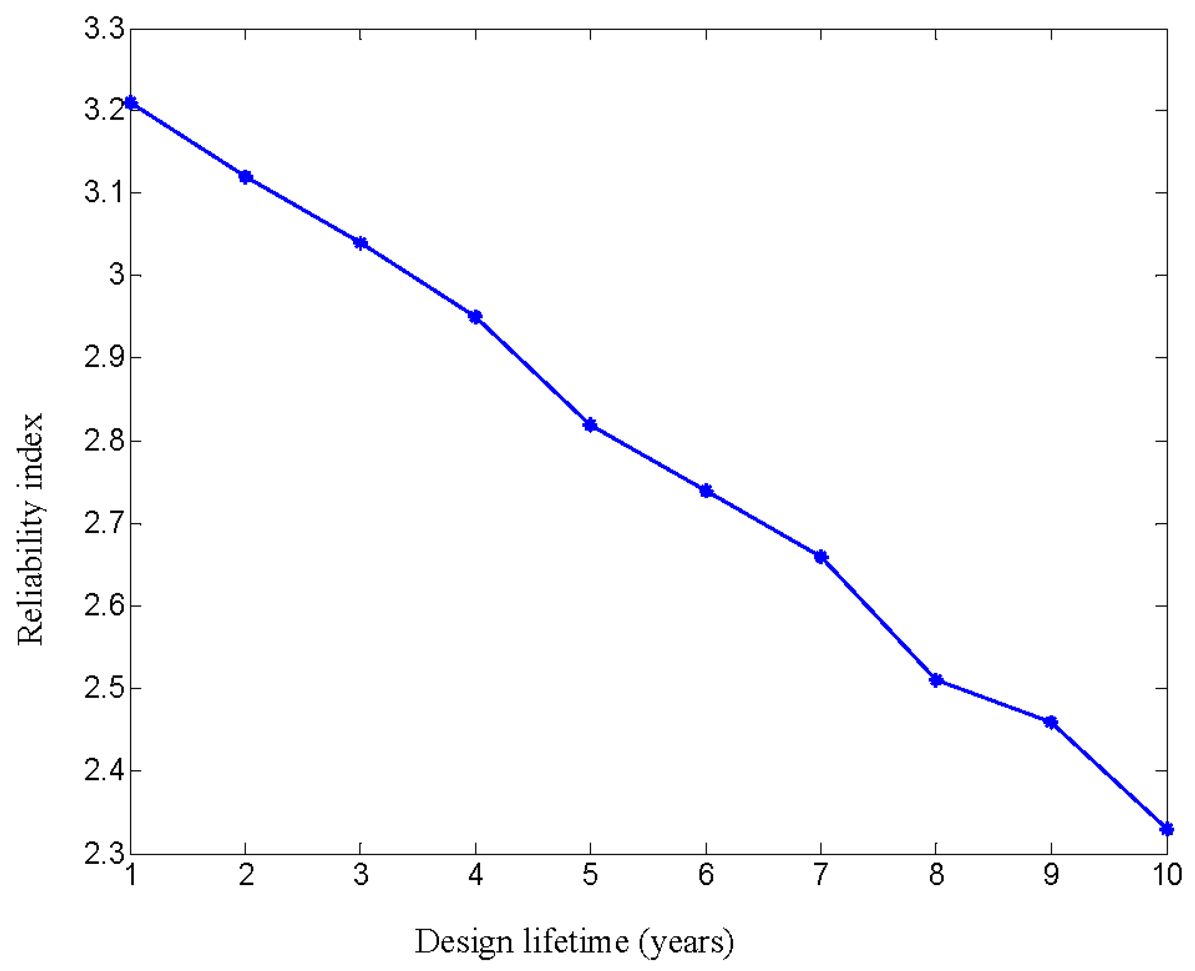
Time/Year	1	2	3	4	5	6	7	8	9	10
Propose method	3.21	3.12	3.04	2.95	2.82	2.74	2.66	2.51	2.46	2.33
Failure probability(10−3)	66	90	118	159	240	307	391	604	695	990

and Figure 7 and Figure 8 show the calculation results. It can be found that when considering the stiffness failure, the reliability of the frame is on the decline. When T = 1, the reliability index is 3.21; when T = 10, the reliability index is 2.33. That means the probability of failure increases. The failure probability is 0.066% in the first year and 0.99% in the tenth year.

5. Conclusions

A time-variant reliability analysis method considering interval variables and stochastic processes is proposed in this paper. This method can handle time-variant reliability calculation when some structural parameters cannot obtain accurate probability distribution due to insufficient samples. By discretizing the stochastic process in time, the time-variant reliability problem is changed into a static hybrid reliability problem. The limit-state function at each time point is expanded at MPP and MUP points. This method avoids the difficulty in solving the crossing rate problem and is easy to understand conceptually. The efficient solution format greatly simplifies the multi-layer nested solution process of time-variant reliability.

The results of numerical example analysis show that the structure’s reliability will not be a fixed value due to the degradation of materials and dynamic uncertain loads but will gradually decrease with the increase of design reference period. Therefore, to ensure the performance of the structure in the whole service period, it is necessary to carry out time-variant reliability analysis of the structure. As the size of time step decreases, the analysis results of the present method approach those of Monte Carlo method. Besides, the approach has high computational efficiency and can satisfy the needs of complex engineering problems. However, this method is mainly applied to the case that the load changes slowly in the time-variant stochastic process. For the dynamic reliability problem that the stochastic process changes violently, the crossing rate method can be used for reliability analysis.

In the future, it is necessary to develop the mixed time-variant reliability of random variables and other uncertain variables, such as fuzzy variables and evidence variables. The hybrid time-varying reliability optimization method is further extended, such as multi-disciplinary reliability design optimization, multi-objective reliability optimization and so on.

References

- Li, F.; Liu, J.; Wen, G.; Rong, J. Extending SORA method for reliability-based design optimization using probability and convex set mixed models. Struct. Multidiscip. Optim. 2019, 59, 1163–1179. [Google Scholar] [CrossRef]
- Li, F.; Liu, J.; Yan, Y.; Rong, J.; Yi, J.; Wen, G. A time-variant reliability analysis method for non-linear limit-state functions with the mixture of random and interval variables. Eng. Struct. 2020, 213, 110588. [Google Scholar] [CrossRef]
- Wu, J.; Zhang, D.; Liu, J.; Jia, X.; Han, X. A computational framework of kinematic accuracy reliability analysis for industrial robots. Appl. Math. Model. 2020, 82, 189–216. [Google Scholar] [CrossRef]
- Liu, J.; Chen, T.; Zhang, Y.; Wen, G.; Qing, Q.; Wang, H.; Sedaghati, R.; Xie, Y. On sound insulation of pyramidal lattice sandwich structure. Compos. Struct. 2019, 208, 385–394. [Google Scholar] [CrossRef]
- Wang, H.; Liu, J.; Wen, G. An efficient evolutionary structural optimization method for multi-resolution designs. Struct. Multidiscip. Optim. 2020, 62, 787–803. [Google Scholar] [CrossRef]
- Zhang, Z.; Li, W.; Yang, J. Analysis of stochastic process to model safety risk in construction industry. J. Civ. Eng. Manag. 2021, 27, 87–99. [Google Scholar] [CrossRef]
- Rice, S.O. Mathematical analysis of random noise. Bell Syst. Tech. J. 1945, 24, 46–156. [Google Scholar] [CrossRef]
- Andrieu-Renaud, C.; Sudret, B.; Lemaire, M. The PHI2 method: A way to compute time-variant reliability. Reliab. Eng. Syst. Saf. 2004, 84, 75–86. [Google Scholar] [CrossRef]
- Sudret, B. Analytical derivation of the outcrossing rate in time-variant reliability problems. Struct. Infrastruct. Eng. 2008, 4, 353–362. [Google Scholar] [CrossRef]
- Hu, Z.; Du, X. Time-dependent reliability analysis with joint upcrossing rates. Struct. Multidiscip. Optim. 2013, 48, 893–907. [Google Scholar] [CrossRef]
- Madsen, P.H.; Krenk, S. An integral equation method for the first-passage problem in random vibration. J. Appl. Mech. 1984, 51, 674–679. [Google Scholar] [CrossRef]
- Jiang, C.; Wei, X.; Huang, Z.; Liu, J. An outcrossing rate model and its efficient calculation for time-dependent system reliability analysis. J. Mech. Des. 2017, 139, 41402. [Google Scholar] [CrossRef]
- Wei, P.; Song, J.; Lu, Z.; Yue, Z. Time-dependent reliability sensitivity analysis of motion mechanisms. Reliab. Eng. Syst. Saf. 2016, 149, 107–120. [Google Scholar] [CrossRef]
- Wang, J.; Gao, X.; Cao, R.; Sun, Z. A multilevel Monte Carlo method for performing time-variant reliability analysis. IEEE Access 2021, 9, 31773–31781. [Google Scholar] [CrossRef]
- Mori, Y.; Ellingwood, B.R. Time-dependent system reliability analysis by adaptive importance sampling. Struct. Saf. 1993, 12, 59–73. [Google Scholar] [CrossRef]
- Wang, J.; Cao, R.; Sun, Z. Importance sampling for time-variant reliability analysis. IEEE Access 2021, 9, 20933–20941. [Google Scholar] [CrossRef]
- Wang, Z.; Mourelatos, Z.P.; Li, J.; Baseski, I.; Singh, A. Time-dependent reliability of dynamic systems using subset simulation with splitting over a series of correlated time intervals. J. Mech. Des. 2014, 136, 61008. [Google Scholar] [CrossRef]
- Li, H.-S.; Wang, T.; Yuan, J.-Y.; Zhang, H. A sampling-based method for high-dimensional time-variant reliability analysis. Mech. Syst. Signal Process. 2019, 126, 505–520. [Google Scholar] [CrossRef]
- Du, W.; Luo, Y.; Wang, Y. Time-variant reliability analysis using the parallel subset simulation. Reliab. Eng. Syst. Saf. 2019, 182, 250–257. [Google Scholar] [CrossRef]
- Hu, Z.; Du, X. Mixed efficient global optimization for time-dependent reliability analysis. J. Mech. Des. 2015, 137, 51401. [Google Scholar] [CrossRef]
- Jiang, C.; Qiu, H.; Gao, L.; Wang, D.; Chen, L. Real-time estimation error-guided active learning Kriging method for time-dependent reliability analysis. Appl. Math. Model. 2020, 77, 82–98. [Google Scholar] [CrossRef]
- Wang, Z.; Chen, W. Time-variant reliability assessment through equivalent stochastic process transformation. Reliab. Eng. Syst. Saf. 2016, 152, 166–175. [Google Scholar] [CrossRef]
- Zhang, D.; Han, X.; Jiang, C.; Liu, J.; Li, Q. Time-dependent reliability analysis through response surface method. J. Mech. Des. 2017, 139, 41404. [Google Scholar] [CrossRef]
- Jiang, C.; Huang, X.; Han, X.; Zhang, D. A time-variant reliability analysis method based on stochastic process discretization. J. Mech. Des. 2014, 136, 91009. [Google Scholar] [CrossRef]
- Du, X. Time-dependent mechanism reliability analysis with envelope functions and first-order approximation. J. Mech. Des. 2014, 136, 81010. [Google Scholar] [CrossRef]
- Gong, J.X.; Zhao, G.F. Reliability analysis for deteriortation structures. J. Build. Struct. 1998, 19, 43–51. (in Chinese). [Google Scholar]
- Jiang, C.; Huang, X.P.; Wei, X.P.; Liu, N.Y. A time-variant reliability analysis method for structural systems based on stochastic process discretization. Int. J. Mech. Mater. Des. 2017, 13, 173–193. [Google Scholar] [CrossRef]
- Jiang, C.; Wei, X.P.; Wu, B.; Huang, Z.L. An improved TRPD method for time-variant reliability analysis. Struct. Multidiscip. Optim. 2018, 58, 1935–1946. [Google Scholar] [CrossRef]
- Cazuguel, M.; Renaud, C.; Cognard, J.Y. Time-variant reliability of nonlinear structures: Application to a representative part of a plate floor. Qual. Reliab. Eng. Int. 2006, 22, 101–118. [Google Scholar] [CrossRef]
- Gong, C.; Frangopol, D.M. An efficient time-dependent reliability method. Struct. Saf. 2019, 81, 101864. [Google Scholar] [CrossRef]
- Ma, Y.; Wang, X.; Wang, L.; Ren, Q. Non-probabilistic interval model-based system reliability assessment for composite laminates. Comput. Mech. 2019, 64, 829–845. [Google Scholar] [CrossRef]
- Qiu, Z.; Huang, R.; Wang, X.; Qi, W. Structural reliability analysis and reliability-based design optimization: Recent advances. Sci. China Phys. Mech. Astron. 2013, 56, 1611–1618. [Google Scholar] [CrossRef]
- Xia, H.; Wang, L.; Liu, Y. Uncertainty-oriented topology optimization of interval parametric structures with local stress and displacement reliability constraints. Comput. Methods Appl. Mech. Eng. 2020, 358, 112644. [Google Scholar] [CrossRef]
- Liu, J.; Wen, G.; Xie, Y.M. Layout optimization of continuum structures considering the probabilistic and fuzzy directional uncertainty of applied loads based on the cloud model. Struct. Multidiscip. Optim. 2016, 53, 81–100. [Google Scholar] [CrossRef]
- Huang, L.; Yin, L.; Liu, B.; Yang, Y. Design and error evaluation of planar 2DOF remote center of motion mechanisms with cable transmissions. J. Mech. Des. 2020, 143, 13301. [Google Scholar] [CrossRef]
- Shi, Y.; Lu, Z. Dynamic reliability analysis model for structure with both random and interval uncertainties. Int. J. Mech. Mater. Des. 2018, 15, 521–537. [Google Scholar] [CrossRef]
- Liu, P.-L.; der Kiureghian, A. Multivariate distribution models with prescribed marginals and covariances. Probab. Eng. Mech. 1986, 1, 105–112. [Google Scholar] [CrossRef]
- Li, C.C.; der Kiureghian, A. Optimal discretization of random fields. J. Eng. Mech. 1993, 119, 1136–1154. [Google Scholar] [CrossRef]
- Ling, C.; Lu, Z. Adaptive kriging coupled with importance sampling strategies for time-variant hybrid reliability analysis. Appl. Math. Model. 2020, 77, 1820–1841. [Google Scholar] [CrossRef]