Abstract
Motivated by the work of Saridakis (Phys. Rev. D 102, 123525 (2020)), the present study reports the cosmological consequences of Barrow holographic dark energy (HDE) and its thermodynamics. The literature demonstrates that dark energy (DE) may result from electroweak symmetry breaking that triggers a phase transition from early inflation to late-time acceleration. In the present study, we incorporated viscosity in the Barrow HDE. A reconstruction scheme is presented for the parameters associated with Barrow holographic dark energy under the purview of viscous cosmology. The equation of state (EoS) parameter is reconstructed in this scenario and quintessence behaviour is observed. Considering Barrow HDE as a specific case of Nojiri–Odintsov (NO) HDE, we have observed quintom behaviour of the EoS parameter and for some values of n the EoS has been observed to be very close to for the current universe. The generalised second law of thermodynamics has come out to be valid in all the scenarios under consideration. Physical viability of considering Barrow HDE as a specific case of NO HDE is demonstrated in this study. Finally, it has been observed that the model under consideration is very close to CDM and cannot go beyond it.
1. Introduction
Gerard ’t Hooft proposed the famous Holographic Principle (HP) inspired by black-hole thermodynamics [1,2]. HP states that all the information contained in a volume of space can be represented as a hologram, which corresponds to a theory located on the boundary of that space [3]. It is widely believed that HP is a fundamental principle of quantum gravity.
In the late 1990s, Reiss et al. [4] and Perlmutter et al. [5] independently reported that the current universe is passing through a phase of accelerated expansion. This started a new era in Modern Cosmology. The authors of [4,5] proved this by observational data. This was further supported by other observational studies [6,7,8,9,10]. Characterised by negative pressure to some exotic matter is thought to be responsible for this acceleration. The exotic matter is dubbed as “dark energy” (DE) [11,12]. It is described by an equation of state (EoS) parameter defined as , where p is the pressure and is the density due to DE. One can easily verify from Friedmann’s equations that is a necessary condition for the accelerated expansion of the universe. The simplest candidate of DE is cosmological constant (), characterised by EoS parameter [13]. Various DE models have been reviewed in the literature [11,12,14,15,16,17,18,19,20,21,22,23,24,25,26]. From References [27,28], currently the DE percentage is . The remaining density is due to dark matter (DM), baryonic matter and radiation. The contributions of baryonic matter and radiation are negligible with respect to the total density of the universe. Dimopoulos and Markkanen [29] have demonstrated that it is possible to obtain DE from the interplay of Higgs boson and inflation, and it has further been demonstrated that a key element for the same result is the electroweak symmetry breaking that can lead to a transition to inflation to late-time acceleration.
One of the broad types of DE candidates is Holographic DE (HDE), which is discussed in References [30,31,32,33,34,35]. The principle of HDE is HP. Its density is given by [31,36,37], where represents a dimensionless constant, is the reduced Planck mass and L stands for infrared (IR) cut-off. To date, there are different modifications in IR cut-off being made. HDE can be accounted for also using corrections without barotropic fluids, for example [38,39]. Observational constraints on DE and HDE can be also found in [40]. In this paper, we will study the Barrow Holographic DE.
In the Covid 19 pandemic, Barrow was very much inspired by its illustrations and deduced that intricate, fractal features on the black-hole structure may be introduced by the quantum-gravitational effects [41]. This complex structure leads to infinite/finite area but with finite volume. Therefore, the entropy expression to a deformed black-hole is [41]
where A is the standard horizon area and is the Planck area. The quantum gravitational deformation is quantified by and corresponds to the standard Bekenstein–Hawking entropy. In addition, corresponds to the most intricate and fractal structure. Note that the usual “ quantum-corrected” entropy with logarithmic corrections is very much different than the “above quantum-gravitationally corrected entropy ”. No doubt, the involved foundation and physical principles are completely different but resemble Tsallis non- extensive entropy.
Gordon M. Barrow quoted “Thermodynamics should be built on energy not on heat and work” [42,43,44,45,46]. The standard HDE is given by , where horizon length and . Therefore, using the Barrow entropy Equation (1) lead to
where C is the parameter with dimension . When , the expression (2) will be standard HDE, i.e., ( is the Planck mass and L is IR cut-off) where and is the model parameter. When the deformation effects quantified by , Barrow HDE will deviate from standard HDE and hence leading to different cosmological consequences. It is very interesting to note that in the limiting case of , the above expression becomes the constant, i.e., .
The concept of viscosity has been analysed from different viewpoints in cosmology [47,48]. The universe consists of various components having different equations of state and cooling rate. Hence, there exist many contexts under which the bulk viscosity causes exponential decay of anisotropy [48]. The viscosity term in the viscosity model dominates the cosmic pressure and exceeds the pressure contribution from other cosmic matter contributions, which contradicts the traditional fluid theory [49]. In this context, let us refer to the extensive review of viscous cosmologies by Medina et al. [50]. In the study of [50], it was demonstrated that bulk viscosity is compatible with the FRW metric and our current study is in line with this. Furthermore, it has been shown by Murphy [51] that the bulk viscosity can lead to a non-singular universe and the consequences of the bulk universe have been discussed in many other studies. In the subsequent sections we are going to demonstrate Barrow HDE under the purview of bulk viscosity and as a specific case of the Nojiri–Odintsov cut-off.
Nojiri and Odintsov [52] developed cosmological models, where the DE and DM were treated as imperfect fluids. Viscous fluids represent one particular case of what was presented in [52]. In the paper, we will incorporate the viscosity term in the various parameters of Barrow HDE. The paper is organised as follows: In Section 2, we will reconstruct the density, thermodynamic pressure of Barrow HDE. We will also reconstruct effective pressure, effective EoS of Viscous Barrow HDE. We will also calculate viscous pressure of Barrow HDE. We will plot density versus ; effective EoS versus redshift z and bulk viscous pressure of viscous Barrow HDE versus redshift z versus C. We will study accordingly. In Section 3, we will study the generalised second law of thermodynamics of viscous Barrow HDE using Barrow entropy. In Section 4, we will reconstruct the density, EoS parameter of Barrow HDE as a Specific NO HDE. We will plot EoS versus redshift z in this case and will study the outcomes. In Section 4.1, we will study the validity of the generalised second law of thermodynamics for Barrow HDE with NO cut-off. Here, we will plot the total entropy of the Barrow HDE with an NO cut-off against the cosmic time t. We give our conclusions in the Concluding Remarks.
2. Viscous Barrow Holographic Dark Energy
In this section we study the effect of viscosity in Barrow HDE. As it is known, viscosity refers to the resistance to flow. By considering many components in the cosmology, there is a contribution of bulk viscosity in the thermodynamic pressure [53], which also plays a very important and crucial role in accelerating the universe. The term bulk viscosity arises because of different cooling rates of the components. We can affirm that the bulk viscous pressure in cosmic media emerges as a result of coupling among the different component of the cosmic substratum [54,55,56,57,58,59,60]. In this context, we would like to mention that in recent years there has been an increased interest in studying cosmic fluid under the purview of bulk viscosity. In a recent work by [61], it has been demonstrated how bulk viscous modifications to the equation of state leads to physically viable results.
Here we will reconstruct the thermodynamic pressure of Barrow HDE with viscosity. Let us assume is the radius of event horizon, then it is given by
or,
Let us assume that infrared (IR) cut-off is the event horizon. Therefore replacing L in Equation (2) with , we get the density of Barrow HDE as
where = radius of event horizon and C is constant. The deformation effect is quantified by . As the DM is in the form of a dust particle, we can consider it as pressureless DM, i.e., . The two Friedmann equations are and , where = Viscous Pressure and .
The conservation equation for pressureless DM is . By solving the expression, we get
Now we are introducing density parameters and and they are given by
and
For , the scenario coincides with cosmology with . Using density parameters from expressions (7) and (8) in the expressions (4) and (5), we obtain
Using from Equation (6) in Equation (7), we obtain
where . Now using the Friedmann Equation and also using Equations (8) and (10), we get
Differentiating Equation (12) with respect to , one gets
where . Equation (13) is the evolution of Barrow HDE in a flat universe for dust matter. For , it coincides with the usual HDE, i.e., . Now from Equation (11), we have
Now using this in Equation (5), we obtain the reconstructed density of Barrow HDE as
As now we have (Equation (16)), H (Equation (14)) and let us take and using these in the conservation equation , we obtain
Therefore, thermodynamic pressure . Hence,
which is the thermodynamic pressure of DE involving the viscous term . As the viscous term is involved here, we can take effective pressure. Hence, effective pressure is Equation (18). As we know the effective Eos, . Thereby, using from Equation (18) and from Equation (16), we get effective EoS as
Now we will insert in , to make it a viscous pressure in Barrow HDE. Now using from Equation (16), from Equation (19) in the conservation equation , we get H. Let us name it as , which is given by
Let us assume the power-law form of scale factor as . As we know that , by using the power-law form of scale factor, we get H. Let us denote this H by , which is given by
It is obvious that is defined for the case , i.e., H will be having singularity at . Now, by using in place of H in i.e., . Then, using this and H as from Equation (20) in , we obtain the viscous pressure in Barrow HDE as
where, , , . Now we will reconstruct a thermodynamic DE pressure i.e., to make it thermodynamic pressure of viscous Barrow HDE. Thus, in the conservation equation , using from Equation (16), from Equation (22), H as from Equation (20), we obtain , which is a thermodynamic pressure of viscous Barrow HDE. Now using Taylor series expansion in the term of Equation (11) and ignoring higher order derivatives, we obtain . From the above equation, we get as
Now, using from Equation (23) in Equation (19), we get and plotted the evolution of effective EoS (19) of viscous Barrow HDE against the redshift z in Figure 1. In this figure, we have made the following choices of parameters: , , , , , , , , . We would like to mention that following Elizalde et al. [62], we have chosen 0.1 km/s/Mpc. In this context we would like to mention that the parameters are not chosen by any standard optimisation technique. Rather, we have confined ourselves to the ranges already mentioned in the existing literature.
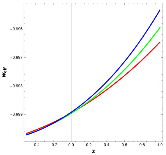
Figure 1.
Evolution of effective equation of state (EoS) (Equation (19)) of viscous Barrow Holographic Dark Energy against redshift z. The red, green and blue lines correspond to , respectively.
From the figure we observe that behaviour of the effective EoS parameter (19) is quintessence. Now we will study the behaviour of (Equation (16)) when . We have plotted the reconstructed density of Barrow HDE against redshift z in Figure 2 for a range of values of .
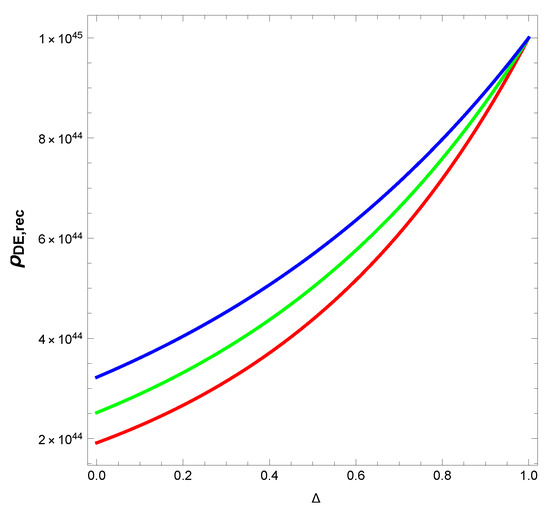
Figure 2.
Evolution of density of Barrow holographic dark energy (HDE) (Equation (16)) against . The red, green and blue line corresponds to , respectively.
In Figure 2 it is observed that density of Barrow HDE has an increasing tendency when the deformation quantifying factor tends to 1. Moreover, at higher values of , the density converges to a point for early current and future universe. This indicates that at that point we can study the evolution of the universe at large for different phases of evolution.
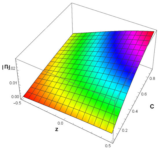
Using the expression of from Equation (23) in the expression of bulk viscous pressure of Barrow HDE , i.e., Equation (22), we have plotted versus redshift z versus C in Figure 3. This figure shows that the constant of Barrow HDE has a significant role to play in the bulk viscous pressure. The effect of bulk viscosity is more for the higher values of C than the lower values. It is further observed that under the current framework the effect of bulk viscosity has a decaying pattern with redshift.
3. Generalised Second Law of Thermodynamics of Viscous Barrow HDE
In this section, we will study the generalised second law of thermodynamics using barrow entropy [46]. We consider the universe horizon to be the boundary of the thermodynamical system. We can take it as an apparent horizon, as it is the most appropriate one. There are many choices in the literature and we chose here the apparent horizon [42,43,44]. The apparent horizon is given by
where k quantifies the spatial curvature and hence , as we considered the universe to be flat. Therefore Equation (24) becomes
From the first Friedmann equation and Equation (25), we get
Now we will check whether the total entropy of the system, i.e., sum of the entropy enclosed by the apparent horizon plus entropy of the apparent horizon of the system is a non-decreasing function of time or not. The apparent horizon is dependent on time. Therefore, changes in apparent horizon in time interval will contribute a change in volume . Hence, the energy and entropy of the system will change by and , respectively. The first law of thermodynamics is . Therefore, the dark energy entropy and dark matter entropy will be [45]:
where DE entropy, DM entropy, DE pressure, DM pressure. V is the universe volume bounded by apparent horizon and is given by . Therefore, . We assume the system to be in equilibrium, so we can consider the temperature of the universe fluids to be same. Dividing Equations (27) and (28) by t, we get
To consider the relationship between thermodynamical quantities and with cosmological quantities and , we use
Now we have , so we can find , from Equation (31), from Equation (32) and hence and . We consider T≈ horizon temperature . Therefore, we can calculate and from Equations (29) and (30), respectively. Now we will calculate horizon entropy . Applying entropy expression to a deformed black hole Equation (1) with standard horizon area , we get , where . Therefore, horizon entropy is given by
Therefore, . After calculating , we plotted it in Figure 4. In this figure, we have considered , , , , , , , , , , . From the figure we have seen that is positive and is non-decreasing. Hence, it satisfies the second law of thermodynamics. This implies the validity of the generalised second law of thermodynamics in the case of viscous Barrow HDE. It is further observed that with evolution of the universe is increasing. This indicates that the validity of the generalised second law of thermodynamics is expected to occur with the evolution of the universe in case of viscous Barrow HDE.
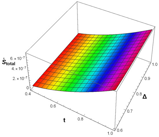
Figure 4.
Plot of of viscous Barrow HDE against the cosmic time t and .
4. Barrow HDE as a Specific NO HDE
In this section, we consider Barrow HDE as a particular case of NO HDE. The NO HDE was proposed in the work of Nojiri and Odintsov [34]. This was further studied in [11]. The DE density for NO HDE is defined as
with
where is the future event horizon discussed in Equations (3) and (4). For the choice of power law form of scale factor , we have IR cut off L as
At this juncture, before passing on to the reconstruction approach let us have an overview of the background of the NO HDE. In this context, it may be noted that Nojiri and Odintsov [34] demonstrated a unifying approach to the early and late-time universe through a phantom cosmology. They considered a gravity-scalar system containing the usual potential and scalar coupling function within the kinetic term. Their study [34] resulted in the possibility of a phantom–non-phantom transition in such a manner that the universe could have the phantom EoS in the early as well as in the late-time. Contrary to the study of [34], our work, a specific case of NO HDE, has led to a quintessence behaviour with no crossing of the phantom boundary; see Figure 1. In this connection, we further note that the generalised HDE with NO cut-off, as proposed in [34], suggested a unified cosmological scenario for tachyon phantoms and for time-dependent phantomic EoS. We further take into account the study of Nojiri and Odintsov [63], where a generalised HDE was proposed with infrared cut-off identified with the combination of the FRW universe parameters. Their study took into account the Hubble rate . However, in our study, we have taken into consideration a Hubble rate , for which we could get a universe where the generalised second law of thermodynamics has come out to be valid. Hence, we can state that the Barrow HDE, a specific case of more general NO HDE can lead to a universe where the generalised second law of thermodynamics is valid. Nojiri et al. [64] established that at late times, the effective fluid can act as the driving force behind the accelerated expansion in the absence of a cosmological constant. Consistent with the findings of [64] in our work on a specific form of NO HDE, the generalised second law appeared to be valid without any cosmological constant. In this context let us mention the work of Nojiri et al. [65], who applied the HP at early times to realise the bounce scenario. The current study with a specific NO HDE cut-off can be further extended to check the realisation of holographic bounce and to study the mechanism of holographic preheating [65] under this framework. Lastly, let us mention the study of Nojiri et al. [66], which confronted the cosmological scenario arising from the application of non-extensive thermodynamics with varying exponents. Their study could provide a description of both inflation and late-time acceleration with the same choices of parameters. We further reiterate that the current Barrow HDE can be examined for its realisation for early inflation and late-time acceleration as a specific case of NO HDE.
Now we demonstrate Barrow HDE as a specific case of NO HDE. In Equations (34)–(36), c, , and are numerical constants and is the constant of integration. Equation (36) represents the NO cut-off as a function of cosmic time t. Now, we consider this NO cut-off as the cut-off for Barrow HDE and from this consideration, we get Barrow HDE generalised by NO HDE and hence, we get the density for Barrow HDE generalised through NO cut-off , which is
We will find the thermodynamic pressure for Barrow HDE generalised through NO cut-off, i.e., from the conservation equation , we get . Hence, the EoS parameter for Barrow HDE generalised through NO cut-off i.e., can be calculated by using from Equation (37) and on equation . In Figure 5, we have plotted the EoS parameter for Barrow HDE as a specific case of NO HDE. In this figure, the evolution of the reconstructed EoS parameter is demonstrated for and the range of values of . It is apparent from this figure that for smaller values of n, the transition from quintessence to phantom is happening at an earlier stage of the universe. However, for , the transition is happening at a later stage. Therefore, in general we can say that the EoS parameter for Barrow HDE reconstructed through NO HDE is characterise by quintom behaviour. Moreover, for , we have for and hence, it is consistent with the observation. Hence, we can conclude that as the IR cut-off for Barrow HDE is reconstructed through NO HDE, the transition from quintessence to phantom is available. It further indicates that under this reconstruction scheme the universe may end with a Big-Rip in the future.
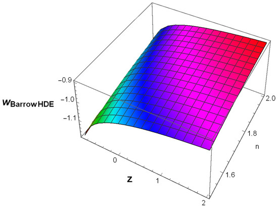
Figure 5.
Evolution of the EoS parameter for Barrow HDE generalised through the Nojiri–Odintsov (NO) cut-off, i.e., against the redshift z and against n.
4.1. Generalised Second Law of Thermodynamics for Barrow HDE with NO Cut-Off
In this subsection, we have studied the generalised second law of thermodynamics for Barrow HDE with NO cut-off using Barrow entropy as in Section 3. We have proceeded similarly as Section 3 just by taking the scale factor as , with . We have calculated the total entropy of the Barrow HDE with NO cut-off, i.e., , and plotted this in Figure 6 against the cosmic time t. In this figure, we have considered , , , , , , , , , , . Figure 6 indicates that is positive and non-decreasing. Therefore, we have observed the validity of the generalised second law of thermodynamics when Barrow HDE is considered as a specific case of NO HDE.
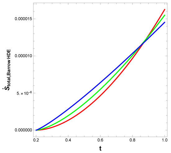
Figure 6.
Plot of of Barrow HDE with NO cut-off against the cosmic time t. The red, green and blue lines correspond to n=, and , respectively.
5. Concluding Remarks
Motivated by the work of Saridakis [41], the present study attempts to probe the cosmological consequences of Barrow HDE and its thermodynamics. In the first phase of the study, we have studied the effect of bulk viscosity in the presence of Barrow HDE. We have reconstructed the density of Barrow HDE as in Equation (16). We also found effective pressure of viscous Barrow HDE as in Equation (18). After finding (Equation (18)), we have derived effective EoS of viscous Barrow HDE as in Equation (19). Thereafter, we calculated viscous pressure in Equation (22) and we also reconstructed thermodynamic pressure of viscous Barrow HDE. In Figure 1, we have plotted (Equation (19)) versus redshift z. From Figure 1, we observed that the behaviour of (Equation (19)) is quintessence. Next, we studied the behaviour of (Equation (16)) as (see Figure 2). It is apparent from this figure that there is an increasing tendency of (Equation (16)) as the deformation quantifying factor , which indicates that we can study the evolution of the universe in its different phases. In addition, we have studied the behaviour of the bulk viscous pressure (Equation (22)) under the purview of Barrow HDE with the evolution of the universe for a range of values of C in Figure 3. The study demonstrated above shows the decaying effect of bulk viscous pressure with the evolution of the universe. Furthermore, the positive impact of the deformation quantifying factor on the bulk viscous pressure is understandable from this figure. This is in contrast with the finding of [67], where the effect of bulk viscosity was found to have an increasing pattern under the purview of holographic Ricci DE.
In Section 3, we have demonstrated the generalised second law of thermodynamics under the purview of the bulk-viscosity of the Barrow HDE. Here, for the study we have taken apparent horizon as the enveloping horizon of the universe. We have calculated the total entropy of the system. The has been plotted in Figure 4, which shows that corresponding to the viscous Barrow HDE is increasing and is staying at a positive level. Therefore, we conclude that the generalised second law of thermodynamics is obeyed by this model [68]. This finding is consistent with the study of [68], where the validity of generalised second law of thermodynamics was examined in the presence of viscous DE and it was observed that the generalised second law of thermodynamics is fulfilled in the presence of bulk viscosity. However, the approach of the current study differs from Setare and Sheykhi [68] in the sense that the standard Eckart approach is adopted here.
In Section 4, we have demonstrated reconstructed schemes of Barrow HDE as a specific NO HDE. We have reconstructed the density, i.e., in Equation (37) for Barrow HDE generalised through NO cut-off. We have also reconstructed the EoS parameter for Barrow HDE generalised through NO cut-off and plotted it in Figure 5. This figure shows the quintom behaviour of . Moreover, at for some values of n. It also suggests that the universe may end with a Big-Rip in the future. Finally, for this reconstructed Barrow HDE we have demonstrated the generalised second law of thermodynamics. For the Barrow HDE with NO cut-off it is observed that (see Figure 6) the time derivative of the total entropy is staying at a positive level and hence, it is concluded that the generalised second law holds if we consider Barrow HDE as a specific case of NO HDE.
While concluding, let us have a look into the reconstructed Barrow HDE for its attainability of a CDM fixed point. It is done through statefinder parameters [69,70] , where q is the deceleration parameter given by . The trajectories in the plane can exhibit different behaviours for different models. The deviation from the point indicates the departure of a model from CDM model. In the present study, the reconstructed Barrow HDE is tested for its deviation from CDM model through the statefinder trajectory plotted in Figure 7 for different values of n. It is observed that this reconstructed Barrow HDE can attain , . Hence, we can conclude that this model is very close to CDM. Furthermore, it is also observed that the statefinder trajectories cannot go beyond the CDM fixed point. In this context, let us comment on the departure of the model from CDM. The attaintment of CDM leads us to interpret that CDM-type cosmology can be reconstructed by Barrow HDE with the Nojiri–Odintsov cut-off in the present formulation that included dark matter. The asymptotic behaviour of density at late times has been observed under this formulation and hence we can interpret that even without a cosmological constant we can reproduce CDM cosmology under the current framework. Hence, we can finally comment that although the current model is deviated from CDM, with appropriate formulation the model can reproduce CDM at late times. However, as the statefinder trajectories could not go beyond the CDM fixed point, we can say that the current model cannot interpolate between dust and CDM.
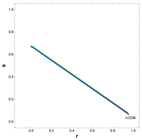
Figure 7.
The statefinder trajectory for the reconstructed Barrow HDE. The CDM fixed point is found to be attainable by the model.
We propose to carry out a similar viscous cosmology under the purview of modified theories of gravity in future with the background evolution as Barrow HDE. While concluding we would like to draw the attention of the readers to the previously published two works [22,23] by the authors of the present paper, where the inflationary cosmology was demonstrated through a scalar field model and a generalised version of HDE. In a similar manner we propose to investigate the slow roll parameters under the consideration of Barrow HDE with NO cut-off as the fluid responsible for the inflationary expansion.
Author Contributions
All authors made equal contributions to the work reported in this paper. All authors have read and agreed to the published version of the manuscript.
Funding
Financial support under the CSIR Grant No. 03(1420)/18/EMR-II is thankfully acknowledged by Surajit Chattopadhyay.
Institutional Review Board Statement
Not applicable.
Informed Consent Statement
Not applicable.
Data Availability Statement
Not applicable.
Acknowledgments
The authors acknowledge the constructive comments from the anonymous reviewers with sincere gratitude. Financial support under the CSIR Grant No. 03(1420)/18/EMR-II is thankfully acknowledged by Surajit Chattopadhyay. Surajit Chattopadhyay and Gargee Chakraborty are thankful to IUCAA, Pune, India, for hospitality during a scientific visit in December 2019-January 2020, when a part of the work was initiated.
Conflicts of Interest
The authors declare no conflict of interest.
References
- Bekenstein, J.D. Black holes and entropy. Phys. Rev. D. 1973, 2333, 7. [Google Scholar] [CrossRef]
- Hawking, S.W. Particle Creation By Black Holes. Commun. Math. Phys. 1975, 199, 43. [Google Scholar] [CrossRef]
- Hooft, G. Dimensional Reduction in Quantam Gravity. arXiv 2009, arXiv:gr-gc/9310026. [Google Scholar]
- Riess, A.G.; Filippenko, A.V.; Challis, P.; Clocchiatti, A.; Diercks, A.; Garnavich, P.M.; Tonry, J. Observational Evidence from Supernovae for an Accelerating Universe and a Cosmological Constant. Astron. J. 1998, 116, 1009. [Google Scholar] [CrossRef]
- Perlmutter, S.; Aldering, G.; Goldhaber, G.; Knop, R.A.; Nugent, P.; Castro, P.G.; Supernova Cosmology Project. Measurements of Ω and Λ from 42 High-Redshift Supernovae. Astrophys. J. 1999, 517, 565. [Google Scholar] [CrossRef]
- Seljak, U.; Makarov, A.; McDonald, P.; Anderson, S.F.; Bahcall, N.A.; Brinkmann, J.; York, D.G. Cosmological parameter analysis including SDSS Lyα forest and galaxy bias: Constraints on the primordial spectrum of fluctuations, neutrino mass, and dark energy. Phys. Rev. D 2005, 71, 103515. [Google Scholar] [CrossRef]
- Astier, P.; Snls Collaboration. The Supernova Legacy Survey: Measurement of OmegaM, OmegaLambda and w from the First Year Data Set. Astron. Astrophys. 2006, 447, 31. [Google Scholar] [CrossRef]
- Abazajian, K.; Adelman-McCarthy, J.K.; Agüeros, M.A.; Allam, S.S.; Anderson, K.S.; Anderson, S.F.; Yocum, D.R. The Third Data Release of the Sloan Digital Sky Survey. Astron. J. 2005, 129, 1755. [Google Scholar] [CrossRef]
- Spergel, D.N. Five-Year Wilkinson Microwave Anisotropy Probe* Observtions: Cosmological Interpretation. Astrophys. J. Suppl. Ser. 2003, 148, 175. [Google Scholar] [CrossRef]
- Komatsu, E.; Dunkley, J.; Nolta, M.R.; Bennett, C.L.; Gold, B.; Hinshaw, G.; Wright, E.L. Five-Year Wilkinson Microwave Anisotropy Probe (WMAP) Observations: Cosmological Interpretation. Astrophys. J. Suppl. 2009, 180, 330. [Google Scholar] [CrossRef]
- Khurshudyan, M. On a holographic dark energy model with a Nojiri-Odintsov cut-off in general relativity. Astrophys. Space Sci. 2016, 361, 232. [Google Scholar] [CrossRef]
- Jawad, A.; Videla, N.; Gulshan, F. Dynamics of warm power-law plateau inflation with a generalized inflaton decay rate: Predictions and constraints after Planck 2015. Eur. Phys. J. C 2017, 77, 271. [Google Scholar] [CrossRef]
- Nojiri, S.; Odintsov, S.D. Inhomogeneous equation of state of the universe: Phantom era, future singularity, and crossing the phantom barrier. Phys. Rev. D 2005, 72, 023003. [Google Scholar] [CrossRef]
- Yu, H.; Ratra, B.; Wang, F.Y. Hubble parameter and Baryon Acoustic Oscillation measurement constraints on the Hubble constant. arXiv 2018, arXiv:1711.03437v2. [Google Scholar]
- Bamba, K.; Capozziello, S.; Nojiri, S.I.; Odintsov, S.D. Dark energy cosmology: The equivalent description via different theoretical models and cosmography tests. Astrophys. Space Sci. 2012, 342, 155–228. [Google Scholar] [CrossRef]
- Nojiri, S.I.; Odintsov, S.D. Final state and thermodynamics of a dark energy universe. Phys. Rev. D. 2004, 70, 103522. [Google Scholar] [CrossRef]
- Nojiri, S.I. Odintsov S.D. Introduction to modified gravity and gravitational alternative for dark energy. Int. J. Geom. Methods Mod. Phys. 2007, 4, 115–145. [Google Scholar] [CrossRef]
- Cognola, G.; Elizalde, E.; Nojiri, S.I.; Odintsov, S.D.; Zerbini, S. Dark energy in modified Gauss-Bonnet gravity: Late-time acceleration and the hierarchy problem. Phys. Rev. D 2006, 73, 084007. [Google Scholar] [CrossRef]
- Capozziello, S.; Cardone, V.F.; Elizalde, E.; Nojiri, S.I.; Odintsov, S.D. Observational constraints on dark energy with generalized equations of state. Phys. Rev. D 2006, 73, 043512. [Google Scholar] [CrossRef]
- Copeland, E.J.; Sami, M.; Tsujikawa, S. Dynamics of dark energy. Int. J. Modern Phys. D 2006, 15, 1753–1935. [Google Scholar] [CrossRef]
- Frusciante, N.; Perenon, L. Effective field theory of dark energy: A review. Phys. Rep. 2020, 857, 1–63. [Google Scholar] [CrossRef]
- Chakraborty, G.; Chattopadhyay, S. Cosmology of a generalised version of holographic dark energy in presence of bulk viscosity and its inflationary dynamics through slow roll parameters. Int. J. Mod. Phys. D 2020, 29, 2050024. [Google Scholar] [CrossRef]
- Chakraborty, G.; Chattopadhyay, S. Modified holographic energy density- driven inflation and some cosmological outcomes. Int. J. Geom. Methods Mod. Phys. 2020, 17, 2050066. [Google Scholar] [CrossRef]
- Chakraborty, G.; Chattopadhyay, S. Investigating inflation driven by DBI-essence scalar field. Int. J. Mod. Phys. D 2020, 29, 2050087. [Google Scholar] [CrossRef]
- Chakraborty, G.; Chattopadhyay, S. Cosmology of Tsallis holographic scalar field models in Chern–Simons modified gravity and optimization of model parameters through χ2 minimization. Z. Naturforsch. 2021, 76, 43–64. [Google Scholar] [CrossRef]
- Chattopadhyay, S.; Chakraborty, G. A reconstruction scheme for f(T) gravity: Variable generalized Chaplygin dark energy gas form. Atron. Nachr. 2021. [Google Scholar] [CrossRef]
- Aghanim, N.; Akrami, Y.; Ashdown, M.; Aumont, J.; Baccigalupi, C.; Ballardini, M.; Roudier, G. Planck 2018 results. VI. Cosmological parameters. Astron. Astrophys. 2020, 641, A6. [Google Scholar]
- NASA. Available online: https://science.nasa.gov/astrophysics/focus-areas/what-is-dark-energy (accessed on 24 March 2021).
- Dimopoulos, K.; Markkanen, T. Dark energy as a remnant of inflation and electroweak symmetry breaking. J. High Energ. Phys. 2019, 2019, 29. [Google Scholar] [CrossRef]
- Li, M. A Model of Holographic Dark Energy. Phys. Lett. B 2004, 603, 1. [Google Scholar] [CrossRef]
- Myung, Y.S. Entropic force and its cosmological implications. arXiv 2011, arXiv:1005.2240. [Google Scholar] [CrossRef]
- Li, M.; Li, X.D.; Wang, S.; Wang, Y.; Zhang, X. Probing interaction and spatial curvature in the holographic dark energy model. JCAP 2009, 0912, 014. [Google Scholar] [CrossRef]
- Nojiri, S.; Odintsov, S.D.; Saridakis, E.N. Holographic inflation. Phys. Lett. B 2019, 797, 134829797. [Google Scholar] [CrossRef]
- Nojiri, S.I.; Odintsov, S.D. Unifying phantom inflation with late-time acceleration: Scalar phantom–non-phantom transition model and generalized holographic dark energy. Gen. Relativ. Gravit. 2006, 38, 1285–1304. [Google Scholar] [CrossRef]
- Nojiri, S.I.; Odintsov, S.D.; Oikonomou, V.K.; Paul, T. Unifying holographic inflation with holographic dark energy: A covariant approach. Phys. Rev. D 2020, 102, 023540. [Google Scholar] [CrossRef]
- Saridakis, E.N.; Bamba, K.; Myrzakulov, R.; Anagnostopoulos, F.K. Holographic dark energy through Tsallis entropy. J. Cosmol. Astropart. Phys. 2018, 2018, 012. [Google Scholar] [CrossRef]
- Elizalde, E.; Nojiri, S.I.; Odintsov, S.D.; Wang, P. Dark energy: Vacuum fluctuations, the effective phantom phase, and holography. Phys. Rev. D 2005, 71, 103504. [Google Scholar] [CrossRef]
- Aviles, A.; Bonanno, L.; Luongo, O.; Quevedo, H. Holographic dark matter and dark energy with second order invariants. Phys. Rev. D 2011, 84, 103520. [Google Scholar] [CrossRef]
- Bueno, P.; Cano, P.A.; Moreno, J.; Murcia, A. All higher-curvature gravities as Generalized quasi-topological gravities. JHEP 2019, 11, 062. [Google Scholar]
- Aviles, A.; Gruber, C.; Luongo, O.; Quevedo, H. Cosmography and constraints on the equation of state of the Universe in various parametrizations. Phys. Rev. D 2012, 86, 123516. [Google Scholar] [CrossRef]
- Saridakis, E.N. Barrow holographic dark energy. Phys. Rev. D 2020, 102, 123525. [Google Scholar] [CrossRef]
- Hayward, S.A. Unified first law of black-hole dynamics and relativistic thermodynamics. Class. Quant. Grav. 1998, 15, 3147–3162. [Google Scholar] [CrossRef]
- Hayward, S.A.; Mukohyama, S.; Ashworth, M. Dynamic black-hole entropy. Phys. Lett. A 1999, 256, 347–350. [Google Scholar] [CrossRef]
- Bak, D.; Rey, S.J. Cosmic holography+. Class. Quant. Grav. 2000, 17, L83. [Google Scholar] [CrossRef]
- Wang, B.; Gong, Y.; Abdalla, E. Thermodynamics of an accelerated expanding universe. Phys. Rev. D 2006, 74, 083520. [Google Scholar] [CrossRef]
- Saridakis, E.N.; Basilakos, S. The generalized second law of thermodynamics with Barrow entropy. arXiv 2006, arXiv:2005.08258v2. [Google Scholar]
- Grøn, Ø. Viscous inflationary universe models. Astrophys. Space Sci. 1990, 173, 191–225. [Google Scholar] [CrossRef]
- Padmanabhan, T.; Chitre, S.M. Viscous universes. Phys. Lett. A 1987, 120, 433–436. [Google Scholar] [CrossRef]
- Xu, D.; Meng, X.H. Bulk Viscous Cosmology: Unified Dark Matter. Adv. Astron. 2010, 2011, 829340. [Google Scholar]
- Medina, S.B.; Nowakowski, M.; Batic, D. Viscous Cosmologies. Class. Quantum Grav. 2019, 36, 215002. [Google Scholar] [CrossRef]
- Murphy, G.L. Big-Bang Model without Singularity. Phys. Rev. D 1973, 8, 4231. [Google Scholar] [CrossRef]
- Nojiri, S.; Odintsov, S.D. The new form of the equation of state for dark energy fluid and accelerating universe. Phys. Lett. B 2006, 639, 144. [Google Scholar] [CrossRef]
- Meng, X.-H.; Dou, X. Singularities and Entropy in Bulk Viscosity Dark Energy Model. Commun. Theor. Phys. 2011, 56, 957. [Google Scholar] [CrossRef]
- Ren, J.; Meng, X.-H. Modified equation of state, scalar field and bulk viscosity in friedmann universe. Phys. Lett. B 2006, 636, 5–12. [Google Scholar] [CrossRef]
- Sharif, M.; Rani, S. Viscous Dark Energy in f(T) Gravity. Mod. Phys. Lett. A. 2013, 28, 1350118. [Google Scholar] [CrossRef]
- Brevik, I.; Grøn, Ø.; de Haro, O.; Odintsov, S.D.; Saridakis, E.N. Viscous cosmology for early-and late-time universe. Int. J. Modern Phys. D 2017, 26, 1730024. [Google Scholar] [CrossRef]
- Brevik, I.; Odintsov, S.D. Cardy-Verlinde entropy formula in viscous cosmology. Phys. Rev. D 2002, 65, 067302. [Google Scholar] [CrossRef]
- Brevik, I.; Gorbunova, O. Dark energy and viscous cosmology. Gen. Relativ. Gravit. 2005, 37, 2039–2045. [Google Scholar] [CrossRef]
- Brevik, I.; Elizalde, E.; Nojiri, S.I.; Odintsov, S.D. Viscous little rip cosmology. Phys. Rev. D 2011, 84, 103508. [Google Scholar] [CrossRef]
- Cruz, M.; Lepe, S.; Odintsov, S.D. Thermodynamically allowed phantom cosmology with viscous fluid. Phys. Rev. D 2018, 98, 083515. [Google Scholar] [CrossRef]
- Brevik, I.; Normann, B.D. Remarks on Cosmological Bulk Viscosity in Different Epochs. Symmetry 2020, 12, 1085. [Google Scholar] [CrossRef]
- Elizalde, E.; Khurshudyan, M.; Odintsov, S.D.; Myrzakulov, R. Analysis of the H0 tension problem in a universe with viscous dark fluid. Phys. Rev. D 2020, 102, 123501. [Google Scholar] [CrossRef]
- Nojiri, S.; Odintsov, S.D. Covariant Generalized Holographic Dark Energy and Accelerating Universe. Eur. Phys. J. C 2017, 77, 8. [Google Scholar] [CrossRef]
- Nojiri, S.; Odintsov, S.D.; Saridakis, E.N.; Myrzakulov, R. Correspondence of cosmology from non-extensive thermodynamics with fluids of generalized equation of state. Nucl. Phys. B 2020, 950, 114850. [Google Scholar] [CrossRef]
- Nojiri, S.; Odintsov, S.D.; Saridakis, E.N. Holographic bounce. Nucl. Phys. B 2019, 949, 114790. [Google Scholar] [CrossRef]
- Nojiri, S.; Odintsov, S.D.; Saridakis, E.N. Modified cosmology from extended entropy with varying exponent. Eur. Phys. J. C 2019, 79, 242. [Google Scholar] [CrossRef]
- Chattopadhyay, S. Viscous extended holographic Ricci dark energy in the framework of standard Eckart theory. Modern Phys. Lett. A 2016, 31, 1650202. [Google Scholar] [CrossRef]
- Setare, M.R.; Sheykhi, A. Viscous dark energy and generalized second law of thermodynamics. Int. J. Modern Phys. D 2010, 19, 1205–1215. [Google Scholar] [CrossRef]
- Sahni, V.; Saini, T.D.; Starobinsky, A.A.; Alam, U. Statefinder—A new geometrical diagnostic of dark energy. JETP Lett. 2003, 77, 201–206. [Google Scholar] [CrossRef]
- Alam, U.; Sahni, V.; Saini, T.D.; Starobinsky, A.A. Exploring the expanding Universe and dark energy using the statefinder diagnostic. Mon. Not. R. Astron. Soc. 2003, 344, 1057–1074. [Google Scholar] [CrossRef]


Publisher’s Note: MDPI stays neutral with regard to jurisdictional claims in published maps and institutional affiliations. |
© 2021 by the authors. Licensee MDPI, Basel, Switzerland. This article is an open access article distributed under the terms and conditions of the Creative Commons Attribution (CC BY) license (http://creativecommons.org/licenses/by/4.0/).