Article

Salt and Pepper Noise Removal Method Based on a Detail-Aware Filter

1
College of Computer Science and Technology, Qilu University of Technology (Shandong Academy of Sciences), Jinan 250023, China
2
Shandong Computer Science Center (National Supercomputing Center in Jinan), Jinan 250101, China
*
Author to whom correspondence should be addressed.
Symmetry 2021, 13(3), 515; https://doi.org/10.3390/sym13030515
Submission received: 27 February 2021 / Revised: 16 March 2021 / Accepted: 18 March 2021 / Published: 21 March 2021
(This article belongs to the Section Computer)

Abstract

:
The median-type filter is an effective technique to remove salt and pepper (SAP) noise; however, such a mechanism cannot always effectively remove noise and preserve details due to the local diversity singularity and local non-stationarity. In this paper, a two-step SAP removal method was proposed based on the analysis of the median-type filter errors. In the first step, a median-type filter was used to process the image corrupted by SAP noise. Then, in the second step, a novel-designed adaptive nonlocal bilateral filter is used to weaken the error of the median-type filter. By building histograms of median-type filter errors, we found that the error almost obeys Gaussian–Laplacian mixture distribution statistically. Following this, an improved bilateral filter was proposed to utilize the nonlocal feature and bilateral filter to weaken the median-type filter errors. In the proposed filter, (1) the nonlocal strategy is introduced to improve the bilateral filter, and the intensity similarity is measured between image patches instead pixels; (2) a novel norm based on half-quadratic estimation is used to measure the image patch- spatial proximity and intensity similarity, instead of fixed L1 and L2 norms; (3) besides, the scale parameters, which were used to control the behavior of the half-quadratic norm, were updated based on the local image feature. Experimental results showed that the proposed method performed better compared with the state-of-the-art methods.

1. Introduction

Detail restoration is a challenging problem that is necessary for some image processing tasks, such as feature extraction, object identification, and pattern recognition. The impulse noise remains in the process of image acquisition and transmission [1,2], which is an inevitable and unwanted phenomenon. The salt and pepper (SAP) noise is a type of impulse noise where the corrupted pixel takes either the maximum or minimum gray value. This noise appears as white and black pixels in the corrupted image [3,4,5]. Moreover, the challenge in detail restoration is further amplified when the images are corrupted by heavy SAP noise owing to the significant destruction of information detail.
In this work, a two-step SAP noise removal method is proposed. The aim of this method is to study the denoising result of the median-type filter further, and propose a novel method to improve the visual quality. First, by analyzing the error of the median-type filter, it was observed to adhere to a Gaussian–Laplacian mixture distribution statistically. Following this observation, in the second step, an adaptive nonlocal bilateral filter has been proposed to utilize the nonlocal feature and bilateral filter to recover the result of median-type filters. In the proposed filter, the difference between the image patch is measured by a modified version of the adaptive norm proposed in [6], which is different from the traditional methods. Moreover, the scale parameters, which were used to control the behavior of the adaptive norm, were updated based on the local feature for higher estimation accuracy.
The contributions of this paper are summarized as follows:
(1)
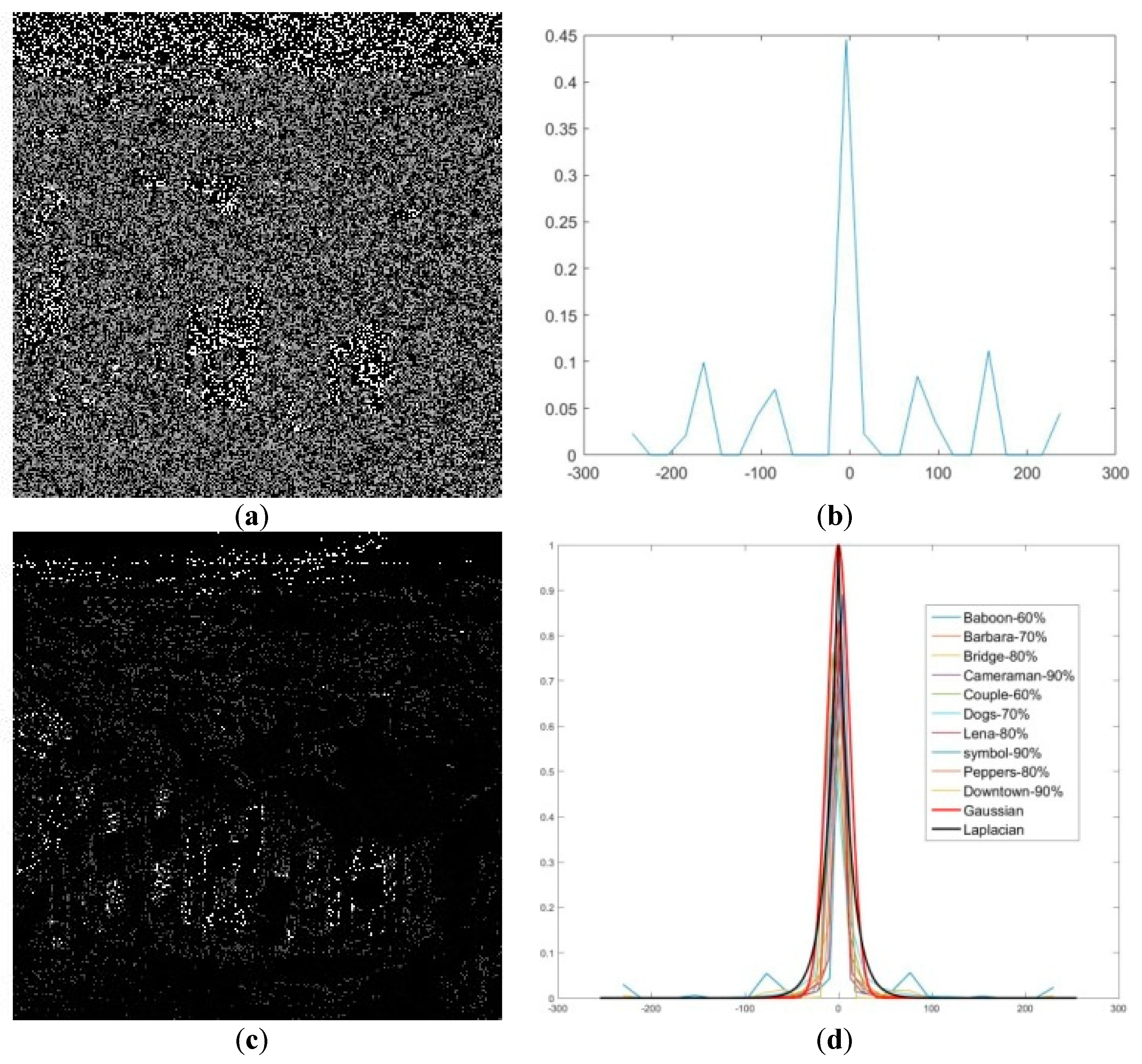
By analyzing the error of the median-type filter statistically, it is found that the error is almost a Gaussian–Laplacian mixture distribution. Therefore, a two-step noise removal method is designed to remove the SAP noise.
(2)
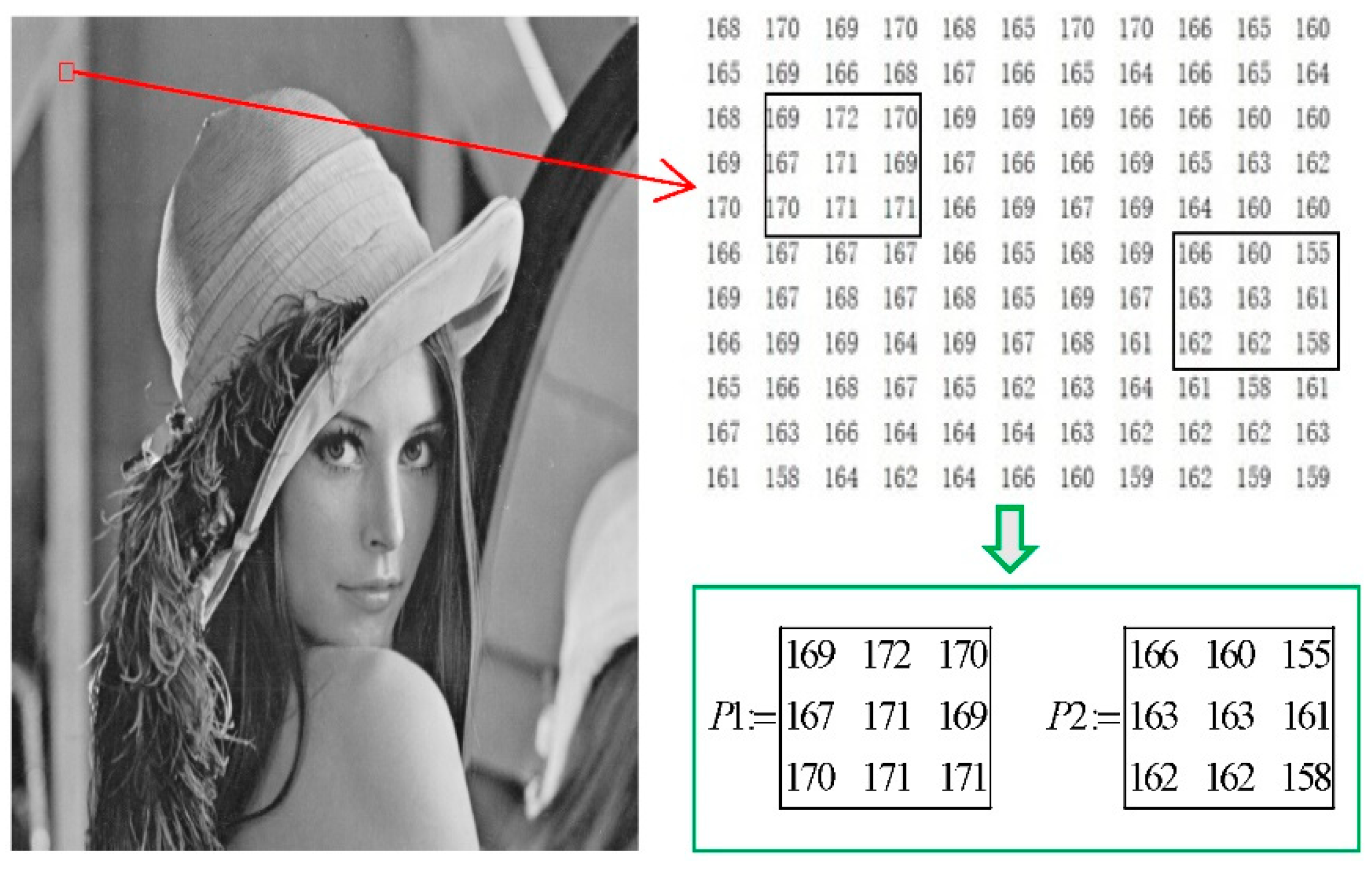
A novel adaptive non-local bilateral filter is proposed to recover the median-type filtered result. Owing to the drawbacks of traditional bilateral filter, a nonlocal operator is used to extract image patches, and the adaptive norm is used to measure the spatial proximity and intensity similarity between the patches.
(3)
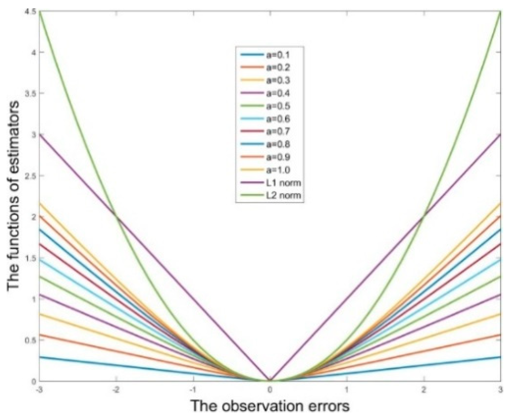
We propose a method to calculate the scale parameters in the adaptive norm. Using this strategy, the context information can be utilized to make the norm adapt to the patch feature.

2. Related Work

There are several methods proposed to reconstruct images corrupted by SAP noise in the past. The research for nonlinear filter is actively pursued in the field of SAP noise removal. Median-type filters [7,8,9,10] are the most popular nonlinear filters. Such as the standard median filter (MF), which is one of the most popular nonlinear filters. MF convolves a moving window with determined size over the image. If the pixel at the center of the window is noisy, its value is replaced with the current window’s median value. However, the noise-free pixels are treated similar to the noisy pixels when these filters are used to restore the corrupted image. These pixels are also replaced with estimated values, which lead to artifacts and blurring. This results in (1) the distortion of original image details and (2) the increase in the computation, especially in the case of low signal–noise ratio.

2.1. Switching Filters

To solve this problem, the switching median-type filters are proposed. The main idea of switching filters is to use a switching process to select the optimal output in the noise detection step or correction step. In [11], first, the authors propose impulse noise detection methods based on evidential reasoning. Then, they design an adaptive switching median filtering which could adaptively determine the size of filtering window according to detection results. The quaternion switching vector median filter, introduced in [12], detects impulse noise based on a quaternion-based color distance and local reachability density. The quaternion-based color distance is used to calculate the local density of a color pixel. Chanu and Singh [13] also propose a switching vector median filter based on quaternion to remove impulse noise, which contains two stages. In the first stage, they use a rank strategy to determine whether the central pixel of the filtering window is noisy pixel or not. Then, in the second stage, the probably corrupted candidate is re-confirmed by using four Laplacian convolution kernels. The noisy pixel is processed by a switching vector median filter based on the quaternion distance.

2.2. Decision Filters

The decision-based method has attracted significant attention for removing SAP noise. Decision filters assume that noisy pixels have a value of 0 or 255 while noise-free pixels have a value between them. As presented in [14], a new filter is established on decision-based filters. The method contains noise detection and restoration. In restoration phase, the uncorrupted pixels keep unchanged and corrupted pixels are interpolated from surrounding uncorrupted pixels using a two-dimensional scattered data interpolation, named natural neighbor Galerkin method. In [15], the noise-free pixels are also left unprocessed and the noisy pixels are replaced with the Kriging interpolation value. The noisy pixels are interpolated from the noise-free pixels in a confined neighborhood. The weights of contributors are calculated using semi-variance between the corrupted pixels and uncorrupted pixels. Besides, an adaptive window size is used for the increasing noise densities.

2.3. Fuzzy Filters

Toh and Isa [16] propose the noise adaptive fuzzy switching median filter (NAFSMF), which is a hybrid between the simple adaptive median filter [17] and the fuzzy switching median filter [18]. NAFSMF contains two stages: noise detection and removal. In the detection stage, the histogram of the corrupted image is utilized to identify noisy pixels. In the removal stage, fuzzy reasoning is employed to deal with uncertainty and design a correction term to estimate noisy pixels. In [19], the authors first improve the maximum absolute luminance difference (ALD) method for detecting noisy pixels more accurately, which helps to classify the pixels into three categories: uncorrupted ones, lightly corrupted ones, and heavily corrupted ones. To restore corrupted pixels, a distance relevant adaptive fuzzy switching weighted mean filter is implemented to remove noise. Afterward, the uncertainty present in the extracted local information as introduced by noise is handled via fuzzy reasoning [20,21].

2.4. Morphological Filters

Morphological filters are non-linear and it can modify the geometrical features locally [22,23]. Mediated morphological filters, introduced in [23], are a combination of median filtering and classical gray-scale morphological operators. After, the mediated morphological filters are applied to remove noise from adult and fetal electrocardiogram (ECG) signal [24,25] and medical images [26]. In [24], mediated morphological filters are used as an efficient preprocessing step to deal with adult and fetal ECG signals. Such a strategy could suppress noise effectively and show low sensitivity to the changes of the structuring element’s length. Compared with [24], the method presented in [25] further concludes the preprocessing result by employing a morphological background normalization. In [26], the mediated morphological filter ability is verified in removing SAP noise, Gaussian noise and Speckle noise from medical images. Compared with the weighted MF, classical MF, and linear filter, the mediated morphological filter shows better performance, even in high abnormal condition of each kind of noise.

2.5. Cascade Filters

The cascade methods use the idea of combining different filters to improve the restoration quality. Such as, the authors of [27] combine the switching adaptive median with fixed weighted mean filter (SAMFWMF). This filter contains switching adaptive median filtering and fixed weighted mean filtering with additional shrinkage window. This filter can achieve optimal edge detection and preservation. In [28], a decision-based median filter is combined with asymmetric trimmed mean filter. In this method, the pixel whose value is equal to 0 or 255 is replaced with the median of the moving window; otherwise, it is replaced with the mean of the window. Raza and Sawant [29] combine a decision-based median filter with a modified decision-based partially trimmed global mean filter (DBPTGMF). Esakkirajan et al. [30] combine a decision-based median filter with a modified decision-based unsymmetrical trimmed median filter (MDBUTMF). Both DBPTGMF and MDBUTMF contain two stages. The first stage is common for both approaches: detect the noisy pixels and replace them with the window’s median. Two main differences exist in the second stage: (I) when detecting the corrupted pixels in the window, if all the pixels in the window (except for the central corrupted pixel) are 0 s (or 1 s), DBPTGMF replaces the corrupted pixel with 0 (or 1). On the other hand, MDBUTMF replaces the corrupted pixel with the window’s mean. (II) If the pixels in the window are a combination of 0 s and 1 s, DBPTGMF replaces the corrupted pixel with the mean of the window. However, the corrupted pixel will be replaced with the median of the window if at least one pixel in the window is different from 0 or 1. For both cases, MDBUTMF replaces the corrupted pixel with the median of the window.

2.6. Nonlocal Means Filter and Bilateral Filter for SAP Noise Removal

Most of the existing SAP noise removal methods are pixel-based methods, which consider the image pixels in a fixed local region only and ignore the image self-similar information. Thus, the image nonlocal structure or the texture structure cannot be preserved properly. To solve this problem, Wang et al. [31] propose the iterative nonlocal means (INLM) filter to remove SAP noise. In this method, switching median filter is first used to mark the pixels as noisy or noise-free pixels and performs filtering on the noisy pixels only. Then, an iterative nonlocal means framework is used to estimate the noisy pixels. In [31], they iteratively exploited the nonlocal similarity feature of the image. They also obtain higher accuracy by updating the similarity weights and the estimated values simultaneously. The bilateral filter is a widely used method for Gaussian noise suppression, and it is barely discussed for SAP noise removal. Veerakumar et al. [32] propose an adaptive bilateral filter by modifying the spatial proximity-based and intensity similarity-based Gaussian function. In the intensity similarity-based Gaussian function, the difference between different pixels is measured by the L2 norm, which penalizes the high-frequency component, and this may blur the edge and texture.

3. Error Analysis and Bilateral Filter

3.1. Error Analysis

In this work, we focused on the statistical characteristics of the results other than the method itself. Based on this idea, we first add salt and pepper noise with various intensities to the image and then remove the noise using the median type filter (i.e., MF, NAFSM)
I ^ m f = M e d i a n F i l t e r ( I )
where I ^ m f denotes the filtered image and I is the image corrupted by the SAP noise. Then, we calculated the error image
I e r r = I ^ m f I o r i
where I e r r is the error image between the filtered image I ^ m f and the original image Iori.
Then, we compute the normalized histogram for the error image. Take the image “Lena” as an example, Figure 1a is the error image between I and the original image Iori, Figure 1b is the histogram for Figure 1a, Figure 1c is the error image between the filtered image I ^ m f and the original image Iori. To verify our hypothesis, we repeated these experiments in different images with different sizes and noise intensities. Furthermore, the histogram of the error of these images is shown in Figure 1d. It can be seen that the curves corresponding to different images are all very close to the red curve (i.e., Gaussian distribution defined in Equation (3)) at both ends, while close to the black curve (i.e., Laplacian distribution defined in Equation (4)) near the peak area. It means that after prefiltering, the noise remained in the image obeys a Gaussian–Laplacian mixture distribution.
If r obeys Gaussian distribution, i.e., r ~ Ν ( μ G , σ G ) , the distribution function is defined as
ρ G ( r ) = 1 2 π σ G exp ( ( r μ G ) 2 2 σ G 2 )
If t obeys Laplacian distribution, i.e., t ~ L a ( μ L , σ L ) , the distribution function is defined as
ρ L ( t ) = 1 2 σ L exp ( | t μ L | σ L )
where, μ G and μ L are position parameter, σ G and σ L are scale parameters.
Intuitively, we deduce that the image obtained by the median-type filter is similar to an image with mixture noise, which can be written as
I ^ m f = I o r i + n G & L
This phenomenon gives us an inspiration that a better denoising performance would be achieved by successfully designing a Gaussian–Laplacian mixed noise filter and introducing it into a SAP noise removal problem. In this paper, this question will be discussed and satisfactory results are obtained by applying the modified bilateral filter into salt-and-pepper noise removal.

3.2. Bilateral Filter

Bilateral filter [33,34] is a kind of nonlinear filter aimed at edge preservation, since it simultaneously considers spatial proximity and the intensity similarity between image pixels. Mathematically, the corrupted image pixel can be estimated by the weighted average of all the neighborhood pixels as
x ( i , j ) = ( k , l ) B ( i , j ) ω d ( i , j , k , l ) ω r ( i , j , k , l ) I ( k , l ) ( k , l ) B ( i , j ) ω d ( i , j , k , l ) ω r ( i , j , k , l )
where x(i, j) denotes the estimated image pixel located at (i, j), B(i, j) denotes the patch whose center pixel is located at (i, j), I ( k , l ) B ( i , j ) , ω d and ω r are both Gaussian functions to measure the spatial proximity and the intensity similarity, respectively. Formally, these functions can be written as
ω d ( i , j , k , l ) = exp ( ( i k ) 2 + ( j l ) 2 2 σ d 2 )
ω r ( i , j , k , l ) = exp ( I ( i , j ) I ( k , l ) 2 2 2 σ r 2 )
where, σd and σr are smoothing parameters.

4. Proposed Two-Step Algorithm

This section presents a detailed explanation of the proposed two-step SAP noise removal algorithm. In the first step, a median-type filter (i.e., NAFSMF) was used to process the corrupted image. Then, in the second step, a novel-designed adaptive nonlocal bilateral (ANB) filter is used to weaken the error of the median-type filter given that it is found to have a Gaussian-like distribution statistically.

4.1. NAFSMF for Preprocessing

In this stage, the noisy image histogram is utilized so as to estimate the noisy pixels in the image corrupted by SAP noise. The local maximum method [18] is first used to detect the noisy pixels. By using this method, it can avoid mistaking noise free intensities in the noisy image histogram for the noisy intensities in the case of low noise intensity. The local maximum is the first peak encountered when traversing the noisy image histogram in a particular direction. The search is started from both ends of the histogram and directed towards the center of the histogram. Two noise intensities are found and used to identify possible noisy pixels in the image. The two local maximums are denoted as NSalt and NPepper, respectively. A noise mask M is designed as follows to mark the location of noisy pixels
M ( i , j ) = { 0 , I ( i , j ) = N S a l t o r I ( i , j ) = N P e p p e r 1 , o t h e r w i s e
where I(i, j) records the gray value at point (i, j). M(i, j) = 1 denotes that the point (i, j) in I is noise-free; otherwise, M(i, j) = 0 denotes that the point (i, j) in I is a noisy point.
To calculate the noisy point I(i, j), first, define a search window W 2 s + 1 ( i , j ) with size (2s + 1) × (2s + 1)
W 2 s + 1 ( i , j ) = { I ( i + m , j + n ) | m , n ( s , s ) }
Then, T 2 s + 1 ( i , j ) is used to count the number of noise-free pixels in W 2 s + 1 ( i , j )
T 2 s + 1 ( i , j ) = m , n ( s , s ) N ( i + m , j + n )
If T 2 s + 1 ( i , j ) > 1 , the value of the noisy pixel is calculated using
I M e d ( i , j ) = m e d i a n { I ( i + m , j + n ) | M ( i + m , j + n ) = 1 ; m , n ( s , s ) }
If T 2 s + 1 ( i , j ) < t , there is not enough noise-free pixels in the current window. In this case, s + 1 s until T 2 s + 1 ( i , j ) > 1 . Finally, y is used to denote the filtering result and the central pixel y(i, j) is calculated using the equation
y ( i , j ) = ( 1 F ( i , j ) ) I ( i , j ) + F ( i , j ) I M e d ( i , j )
where F(i, j) is a fuzzy membership function that is defined as
F ( i , j ) = { 0 , D ( i , j ) < T 1 D ( i , j ) T 1 T 2 T 1 T 1 < D ( i , j ) < T 2 1 D ( i , j ) > T 2
In Equation (14), D(i, j) represents the local information defined as the maximum gray value difference in a 3 × 3 window, and it is defined as
D ( i , j ) = max { | I ( i + k , j + l ) I ( i , j ) | k , l ( 2 , 2 ) , ( i + k , j + l ) ( i , j ) }

4.2. ANB Filter to Improve Result

The bilateral filter has local characteristics due to considering the pertinence of pixels to estimate noisy pixels. The pertinence will be destroyed when encountering high noise intensity, thus the denoising effect will be greatly reduced. To address this problem, we first introduce the nonlocal strategy to the bilateral filter, and a new function to measure the patch intensity similarity is obtained,
ω ¯ r ( i , j , k , l ) = exp ( y ( p , q ) Θ ( i , j ) y ( r , s ) Θ ( k , l ) Θ ( i , j ) , Θ ( k , l ) Ω ( y ( p , q ) y ( r , s ) ) 2 β )
where, Ω represents the search window, Θ ( i , j ) represents the patch centered by y(i, j), Θ ( k , l ) represents the patch centered by y(k, l), β > 0 is a model parameter.
Suppose the vector v R n , the Lp norm of v is defined as v p = ( i = 1 n | v i | p ) 1 p . For the Gaussian noise and Laplacian noise, L2 norm is an excellent choice. However, the L2 norm is outliers, thus, the L2 norm does not perform as well as the L1 norm in preserving sharp edges. Moreover, when using Equations (7) and (16) based method to deal with the preprocessing result, there still exists some problems, such as, (1) all pixels need to be estimated; (2) all pixels in the search window contribute to the estimation; and (3) fixed L2 norm used in Equation (16) is sensitive to high frequency information, which may blur the image edge. Based on the above analysis, we further modified the spatial proximity-based function and the intensity similarity-based function as
ω ^ d ( i , j , k , l ) = { exp ( ( i k ) 2 + ( j l ) 2 α ) 0
ω ^ r ( i , j , k , l ) = { exp ( y ( p , q ) Θ ( i , j ) y ( r , s ) Θ ( k , l ) Θ ( i , j ) , Θ ( k , l ) Ω φ ( y ( p , q ) y ( r , s ) , a ) β ) 0
where, Ω represents the search window, Θ(i, j) represents the patch centered by y(i, j), Θ(k, l) represents the patch centered by y(k, l), α > 0 and β > 0 are model parameters, φ(t, a) is a measure function defined by φ ( t , a ) = a a 2 + t 2 a 2 with scale parameter a > 0. φ(t, a) has self-adaptability of mimicking L1 and L2 norms, and the parameter a controls the transition from L1 norm to L2 norm. Larger a denotes a larger range of difference values that can be discriminated by the L2 norm. In the two patches, Θ(i, j) and Θ(k, l), the difference y(p, q) − y(r, s) may be variational owing to the location. Thus, using the same a to measure the difference is not an excellent choice. In this work, the parameter a is computed based on the local image feature
a p , q , r , s = 1 ( y ( p , q ) y ( r , s ) ) 2 + ε
where ε > 0, which is used to avoid making the dividend zero. Detail analysis about a p , q , r , s is presented in Section 5.
Thus, by substituting a with Equation (19) in Equation (18), we can obtain new functions for the distance in intensity space
ω ^ r ( i , j , k , l ) = { exp ( y ( p , q ) Θ ( i , j ) y ( r , s ) Θ ( k , l ) ψ ( y ( p , q ) y ( r , s ) , a p , q , r , s ) β ) 0
where ψ ( t , a p , q , r , s ) = a p , q , r , s a p , q , r , s 2 + t 2 a p , q , r , s 2 .
Based on Equations (17) and (20), the ANB filter is proposed and defined as
x ^ ( i , j ) = ( k , l ) Θ ( i , j ) ω ^ d ( i , j , k , l ) ω ^ r ( i , j , k , l ) y ( k , l ) ( k , l ) Θ ( i , j ) ω ^ d ( i , j , k , l ) ω ^ r ( i , j , k , l )
In the following section, we will discuss the advantages of the adaptive norm compared with L1 and L2 norms in theory. The experimental comparisons are also shown in Section 6.

4.3. Proposed Two-Stage Noise Removal Algorithm

In this subsection, we summarized the whole salt and pepper noise removal algorithm. The whole algorithm contains two stages: (1) median-type filter and (2) the proposed ANB filter. The proposed algorithm is described as Algorithm 1:
Algorithm 1: Proposed two-stage noise removal algorithm
Input: noisy image I, α, β;
First stage
 1. Obtain M using Equation (9);
 2. 1 s
  Obtain W 2 s + 1 ( i , j ) and T 2 s + 1 ( i , j ) ;
  Do s s + 1 until T 2 s + 1 ( i , j ) > 1 ;
 3. Calculate I M e d ( i , j ) = m e d i a n { I ( i + m , j + n ) | m , n ( s , , 0 , s ) } ;
 4. Calculate y = ( 1 F ( i , j ) ) I ( i , j ) + F ( i , j ) I M e d ( i , j ) using Equations (14) and (15);
Second stage
 5. Calculate the spatial proximity using
ω ^ d ( i , j , k , l ) = { exp ( ( i k ) 2 + ( j l ) 2 α ) 0
 6. Calculate the scale parameters using
a p , q , r , s = 1 ( y ( p , q ) y ( r , s ) ) 2 + ε
 7. Calculate the intensity similarity using
ω ^ r ( i , j , k , l ) = { exp ( y ( p , q ) Θ ( i , j ) y ( r , s ) Θ ( k , l ) ψ ( y ( p , q ) y ( r , s ) , a p , q , r , s ) β ) 0
 8. Obtain the de-noised result
x ( i , j ) = ( k , l ) Θ ( i , j ) ω ^ d ( i , j , k , l ) ω ^ r ( i , j , k , l ) y ( k , l ) ( k , l ) Θ ( i , j ) ω ^ d ( i , j , k , l ) ω ^ r ( i , j , k , l )
Output: de-noised image x

5. Efficiency Analysis

One of the main contributions of this manuscript is the establishment of the ANB filter, which is based on the improved functions ( ω ^ d and ω ^ r ) with regard to the spatial proximity and the intensity similarity, respectively. The efficiency analysis mainly includes three aspects: (1) the error analysis, which provides an explanation to add the following ANB step; (2) the weight analysis, which shows the efficiency of the introduction of ω ^ d and ω ^ r into the ANB filter; and (3) the norm choice analysis, which presents the efficiency of using the adaptive norm to improve ω ^ r . The error analysis has been presented detailed in Section 2, thus, in this section, the efficiency analysis mainly includes two parts: weight analysis and norm choice.

5.1. Weight Analysis

Two improved weight functions were designed in the proposed filter. The two functions were based on spatial proximity and intensity similarity. The efficiency of using the two weights ω ^ d and ω ^ r was analyzed in three special situations as follows:
Case 1: Considering Equations (17) and (20), if the contributed pixel y(k, l) is corrupted, ω ^ d = ( i , j , k , l ) = 0 and ω ^ r = ( i , j , k , l ) = 0 . To this end, the pixel y(k, l) has no effect on estimating y(i, j). This design can avoid misestimation owing to the corrupted points.
Case 2: If the contributed pixel y(k, l) is noise-free in the smooth region, but y(i, j) in an area where the gray value changes dramatically (i.e., edge region), the difference between the two pixels is large. Correspondingly, the difference between the patches centered by y(k, l) and y(i, j) may be large. In this case, the variable ω ^ r is close to 0, and the value of ω ^ d is small. Thus, it is a double insurance to keep the weight of y(k, l) is small enough when computing for y(i, j).
Case 3: If both y(k, l) and y(i, j) are in the smooth region, a small difference is shown among the image pixels. In this situation, the difference between the patches tends to be 0 infinitely. Thus, the weight ω ^ r approaches 1, and only the weight ω ^ d works. Here, the proposed filter works as a Gaussian filter.

5.2. Norm Choice

The proposed norm ψ ( t , a p , q , r , s ) = a p , q , r , s a p , q , r , s 2 + t 2 a p , q , r , s 2 tends to utilize the advantages of L1 norm and L2 norm, and it has a good adaptivity to the local information by avoiding to set the threshold value to control the selection of the norm compared with other estimators (i.e., the Huber norm, the Leclerc norm, and the Lorentzian norm).
From Equation (19), it is noted that when the difference between y(p, q) and y(r, s) is small, the value of ap,q,r,s is large. Here, the modified adaptive norm contains a range where it performs similar to the L2 norm as large as possible. Conversely, ap,q,r,s is small, and the modified adaptive norm performs similar to the L1 norm, which can remove noise and preserve edges. Thus, the proposed adaptive norm can work as L1 norm or L2 norm automatically according to the local features.
In the following equation,
ψ ( t ) = a p , q , r , s a p , q , r , s 2 + t 2 a p , q , r , s 2 .
where ap,q,r,s is used to control the scope of the linear behavior as shown in Figure 2. This norm is shown in Figure 2 with different ap,q,r,s-values where it can be seen that the adaptive norm gets closer to the L1 norm when the sale parameter tends to zero. Specifically, larger sale parameter results in a larger range of error values that can be discriminated by the linear influence function. Moreover, in ψ ( t ) , the sale parameter controls the transition from L1 norm to L2 norm.
In ω r ( i , j , k , l ) , Equation (8), L2 norm was used to measure the difference between the point y(i, j) and y(k, l). Theoretically, when the difference is large, the weight of y(k, l) is correspondingly small, which means that y(k, l) has little impact on the estimation of y(i, j). Meanwhile, when the difference is very small, especially close to 0, y(k, l) is similar to y(i, j). Here, the L2 norm can enlarge the weight of y(k, l), which increases its contribution to y(i, j). Sometimes, the expected effect may not be achieved using the L2 norm.
The intensity difference in the smooth region tending to be zero is an ideal condition; thus, using the L2 norm to control the weight based on the intensity similarity is not an optimal choice. A simple example is shown in Figure 3 where the region in the red block is an almost smooth area, which is noted as region A. Assuming that y ( i , j ) A , y ( k , l ) A , y(i, j) is a corrupted pixel, and y(k, l) is uncorrupted. Intuitively, y(k, l) should make a large contribution for estimating y(i, j), namely, ω ( i , j , k , l ) 1 , where y(i, j) is the center value of region P1 and y(k, l) is the center value of region P2. However, in the real situation, this assumption could not be achieved because the L2 norm will sharpen the difference. However, the adaptive norm would have a good performance. The analysis is discussed as follows.
Let ω ^ r a d a p t i v e and ω ^ r L 2 denote the Gaussian functions to measure the intensity similarity based on the adaptive norm and L2 norm. Formally, they can be presented as
ω ^ r a d a p t i v e ( i , j , k , l ) = exp ( y ( p , q ) P 1 y ( r , s ) P 2 ψ ( y ( p , q ) y ( r , s ) , a p , q , r , s ) β )
ω ^ r L 2 ( i , j , k , l ) = exp ( y ( p , q ) P 1 y ( r , s ) P 2 ( y ( p , q ) y ( r , s ) ) 2 β )
From these expressions, the difference measurement part of the two formulas is ( ψ ( y ( p , q ) y ( r , s ) , a p , q , r , s ) and ( y ( p , q ) y ( r , s ) ) 2 ). Here, we need to prove that ψ ( y ( p , q ) y ( r , s ) , a p , q , r , s ) < ( y ( p , q ) y ( r , s ) ) 2 with the same σr. For convenience, denote y ( p , q ) y ( r , s ) = t , such that
g ( t ) = a p , q , r , s a p , q , r , s 2 + t 2 a p , q , r , s 2 t 2 = a p , q , r , s 2 + t 2 ( a p , q , r , s a p , q , r , s 2 + t 2 )
Obviously, g(t) < 0, ω ^ r a d a p t i v e ( i , j , k , l ) > ω ^ r L 2 ( i , j , k , l ) . Specifically, using the L2 norm to measure the difference will weaken the contribution of y(k, l), which is contrary to the proposed norm.

6. Experimental Results and Discussion

To evaluate the proposed algorithm, several simulation experiments were performed in this section to compare with many state-of-the-art methods. The noisy images are generated by adding salt and pepper noise with nine different intensities from σ = 10% to σ = 90% to the test images shown in Figure 4, which presents gray-scaled image with sizes between 256 × 256 and 512 × 512. Denoising performance was measured by many subjective and objective standards. The subjective standard included reconstructed images and the corresponding error images. The objective standard included image enhancement factor (IEF) [35], structure similarity index (SSIM) [36], and peak signal-to-noise ratio (PSNR) to evaluate the performance of the proposed method.
In this work, we first compared the proposed method using the adaptive norm with L1 norm- and L2 norm-based methods. Then, we compared the proposed method with eight previous works, including the median filter (MF), adaptive center weighted median filter (ACWMF, 2001) [37], NAFSMF (2010) [16], an edge-preserving approach based on adaptive fuzzy switching median filter (NASEPF, 2011) [38], INLM (2016) [31], different applied median filter (DAMF, 2018) [39], decision-based algorithm (DBA, 2011) [40] and adaptive type-2 fuzzy approach for salt-and-pepper noise (FSAP, 2018) [41].
In the proposed method, the related parameters are set as follows: T1 = 10, T2 = 30, α = 50×noise intensity, β = 50× noise intensity, the similar patch size is 3 × 3, and the searching window size is 7 × 7. For the other methods, the parameters are set for the best performance. All codes were running in MATLAB 2015b using an i7-7500U CPU, 16 GB RAM computer under Microsoft Windows 10 operation system. For each comparison method, all parameters were selected under the declarations in their papers.

6.1. Comparison under Different Norm Choice

We will take Barbara and Man-made images shown in Figure 4 as examples to compare our proposed method with the L1-based method and L2-based method. The main difference between these three methods is the norm used to measure the intensity similarity in the second stage.
Table 1, Table 2 and Table 3 show the PSNR value, SSIM value, and IEF value, respectively. According to the results in Table 1, Table 2 and Table 3, the proposed method outperformed the other two methods in most cases, especially in high-intensity noise. For example, the proposed method performs better than the L1-based method (average PSNR(dB): 0.68, 0.66, and 0.12; average SSIM: 0.0151, 0.0178, and 0.0099; average IEF: 10.93, 5.85, and 1.09) in the case of σ = 70 % , σ = 80 % , and σ = 90 % , respectively. Moreover, the proposed method performs better than the L2-based method (average PSNR(dB): 0.69, 1.1, and 1.1; average SSIM: 0.0029, 0.0132, and 0.0172; average IEF: 6.65, 13.74, and 13.14) in the case of σ = 70 % , σ = 80 % , and σ = 90 % , respectively. The L1-based method has the advantage in edge preserving. However, the detail region would be over-smooth. The L2-based method can remove noise effectively, while it always makes the edges blur. The proposed method is based on an adaptive norm which has self-adaptability of mimicking L1 and L2 norms. Thus, our method can balance the noise removal and detail protection, even in high-intensity noise.

6.2. Comparisons between Pre- and Post-Processed Images

In this sub-section, we would like to show the proposed method effectively reducing the error for a preprocessed image. Figure 5 shows three examples based on Couple, Pepper, and Street images. For better comparisons, we show the error images and the enlarged detail parts. From Figure 5, we can see that the post-processed images have more acceptable details and less error. Besides, the corresponding PSNR, SSIM, and IEF values are presented in Table 4, Table 5 and Table 6.
According to these tales, it can be seen that the post-processed images achieves higher PSNR, SSIM, and IEF values. For example, the post-processed images gains higher values than the pre-processed images (average PSNR(dB): 1.41, 1.68, and 2.72; average SSIM: 0.0320, 0.0432, and 0.1031; average IEF: 36.47, 33.46, and 37.94) in the case of σ = 70 % , σ = 80 % , and σ = 90 % , respectively. This indicates that the proposed method could further reduce the error in the preprocessed images. That is because in the proposed two-stage method a novel bilateral filter is used to weaken the median-type filter errors is effective.

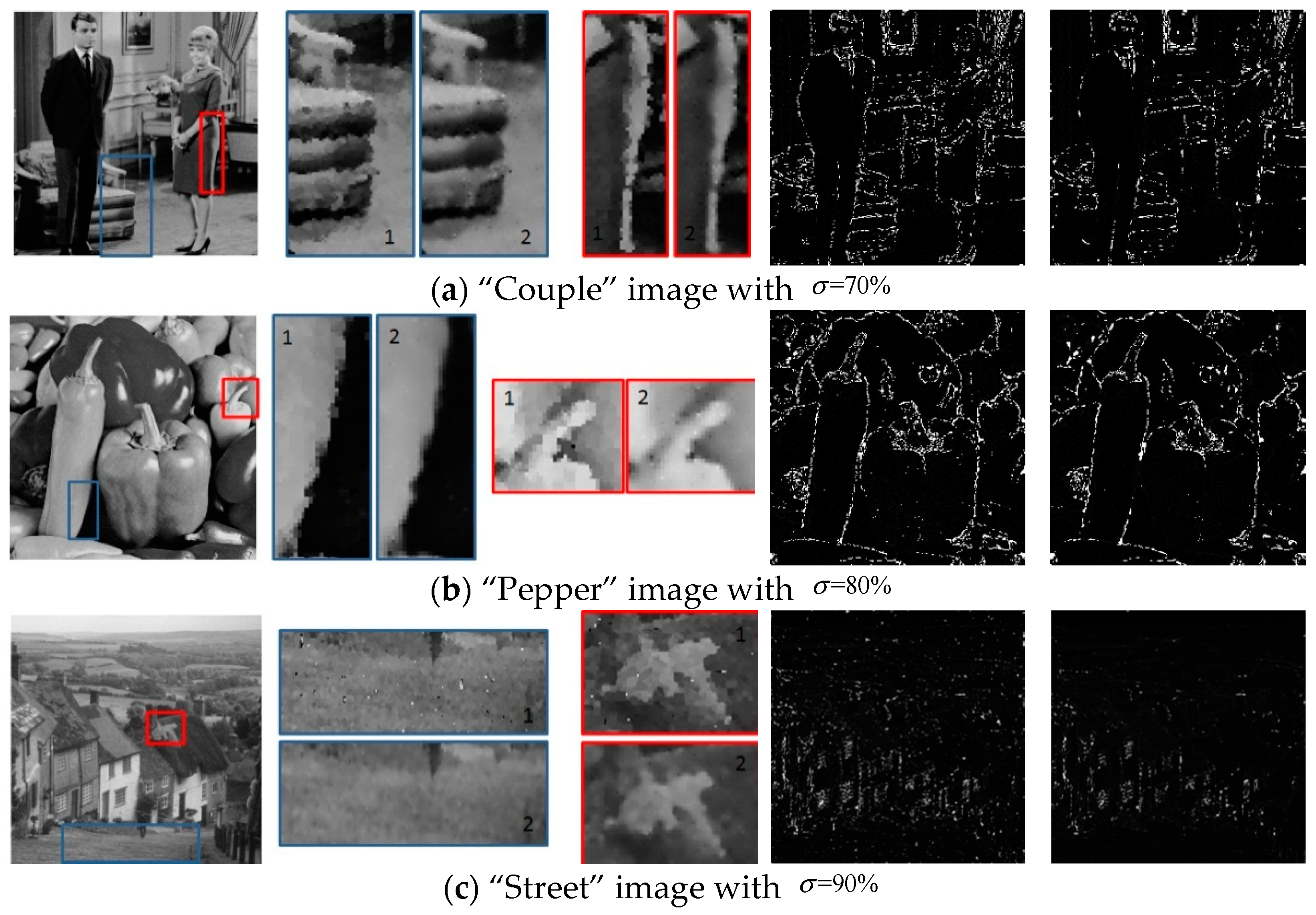
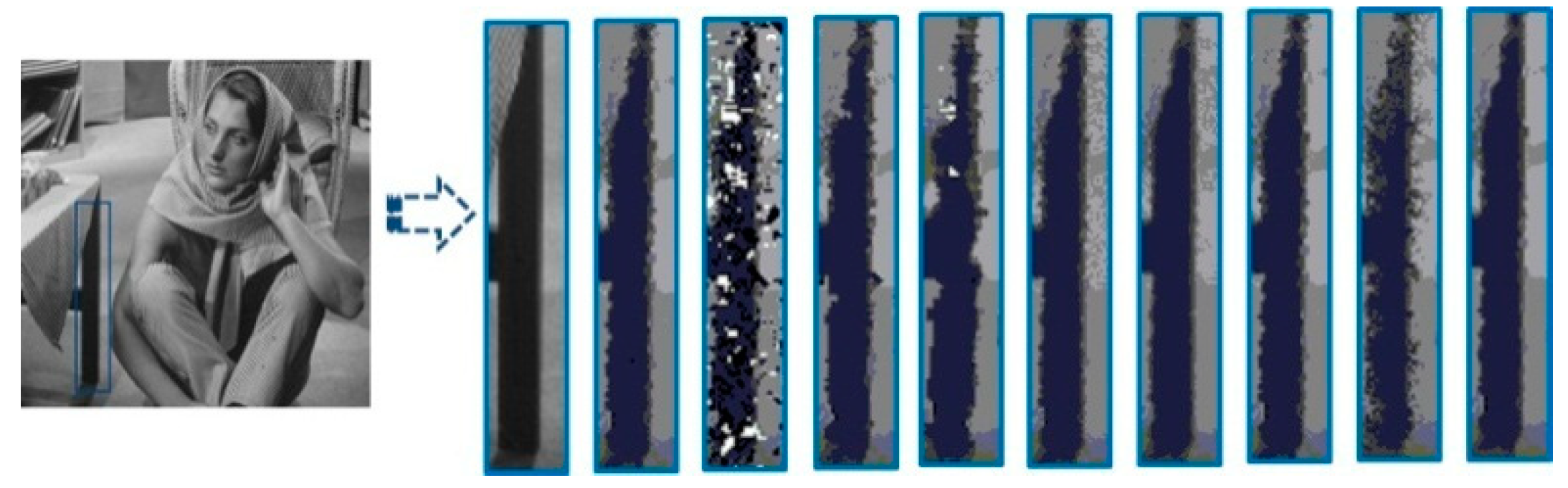
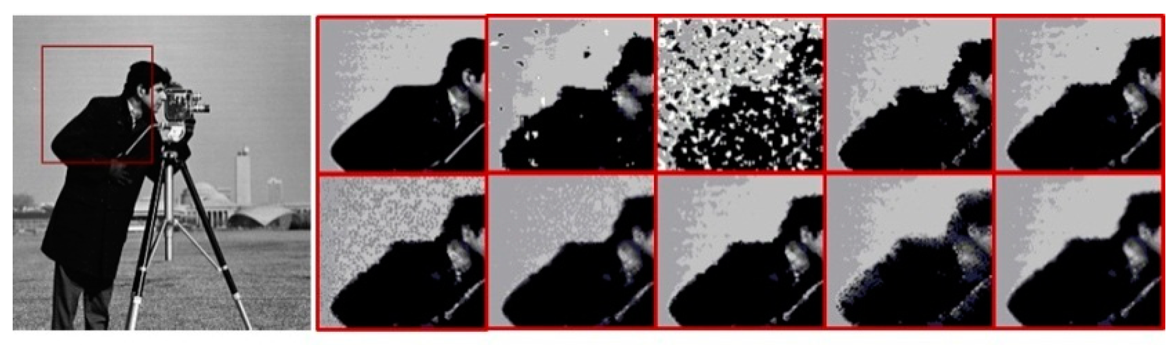
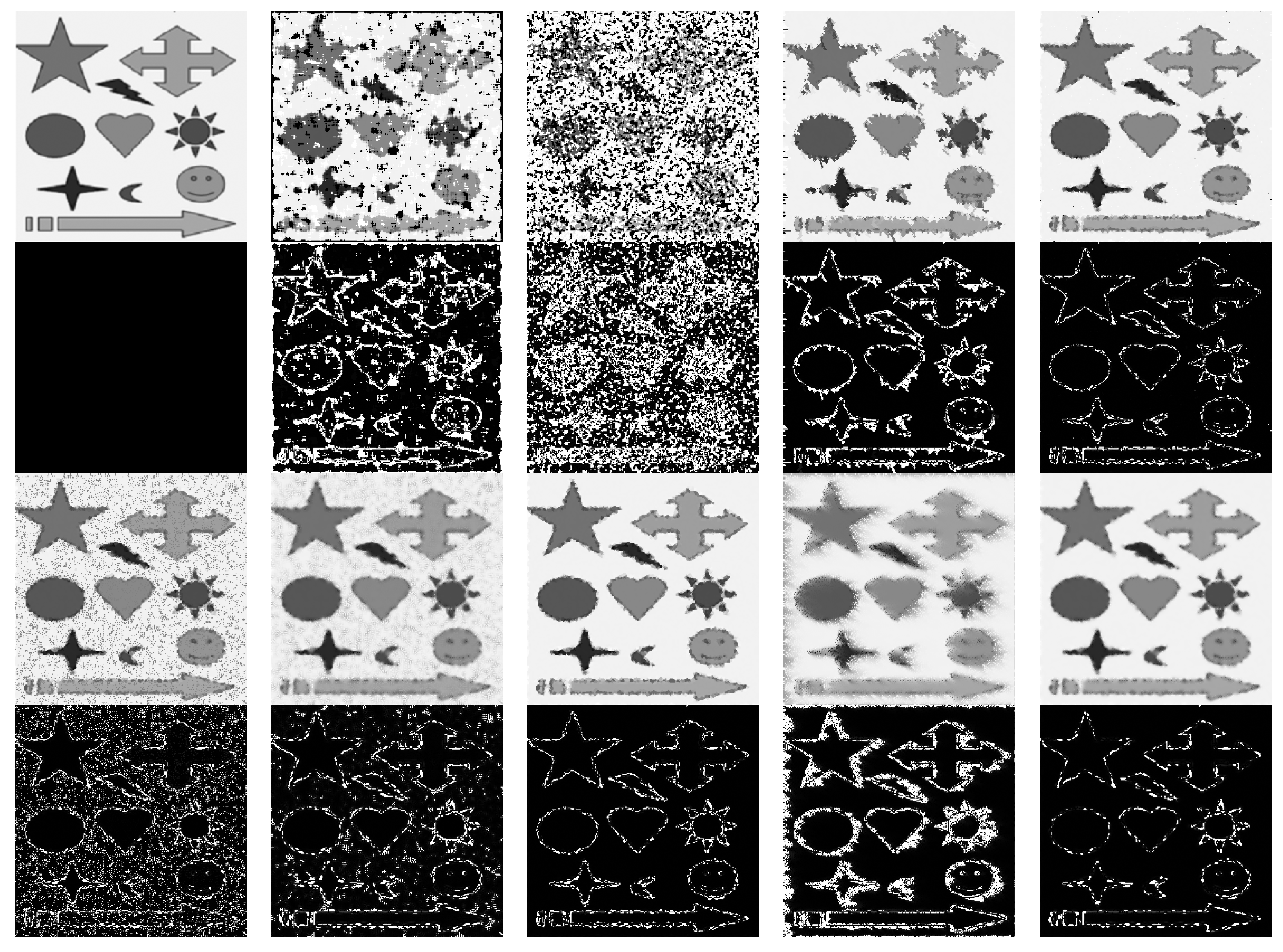
6.3. Subjective Quality Analysis

In this sub-section, three evaluation measures (i.e., PSNR, IEF, and SSIM) were presented to validate the perception-based image quality assessment on different images under different noise levels. We compared the proposed adaptive method with DBA, MF, ACWMF, NASFM, NASEPF, INLM, DAMF, and FSAP. For far comparison, all parameters in each algorithm are under their statements in published papers.
The graphs of IEF for different images with noise levels varying from σ = 10–90% are shown in Figure 6. For the subfigures in Figure 6, x-axis means σ = 10–90% from left to right. The y-axis denotes the IEF value. This figure confirmed that the proposed method obtained better results compared with other considered methods in terms of higher IEF value. Table 7 shows the PSNR values on the restored images corresponding to eight test images, including those shown in Figure 4 with the noise intensity changes from 10% to 90% as well as Table 8 shows the corresponding SSIM values on the restored images. For better comparisons, we have colored the best values into red.
From these tables, we can see that our proposed method gets the highest PSNR and SSIM values both in the low noise intensity and high noise intensity, which demonstrates the efficiency and necessity of incorporating a novel bilateral filter to weaken the median-type filter errors. In the case of low noise intensity, taking σ = 10% as an example, all the methods achieve high PSNR and SSIM values. The PSNR and SSIM values achieved by different methods are shown in the following: MF (22.01 dB, 0.7025), ACWMF (31.20 dB, 0.9524), DBA (35.09 dB, 0.9828), NAFSM (36.71 dB, 0.9807), NASEPF (27.25 dB, 0.8077), INLM (30.52 dB, 0.8750), DAMF (36.93 dB, 0.9850), FSAP (35.56 dB, 0.9831), and OURS (38.15 dB, 0.9865). We can see that in the case of σ = 10%, the PSNR value of the proposed method (38.15 dB) has outperformed that of the MF method, the ACWMF method, the DBA method, the DAMF method, and the FSAP method more than 1.2. Even in the case of σ = 90% (correspondingly a strong noise), the PSNR value of the proposed method (22.81 dB) has outperformed the PSNR values of the MF method, the ACWMF method, the DBA method, the DAMF method, and the FSAP method more than 1.4. In addition, the proposed method also achieves slightly better reconstruction performance than the INLM method (22.27 dB). Compared with the INLM, a novel bilateral filter is proposed in this work, which is more efficient to suppress the Gaussian–Laplacian errors.

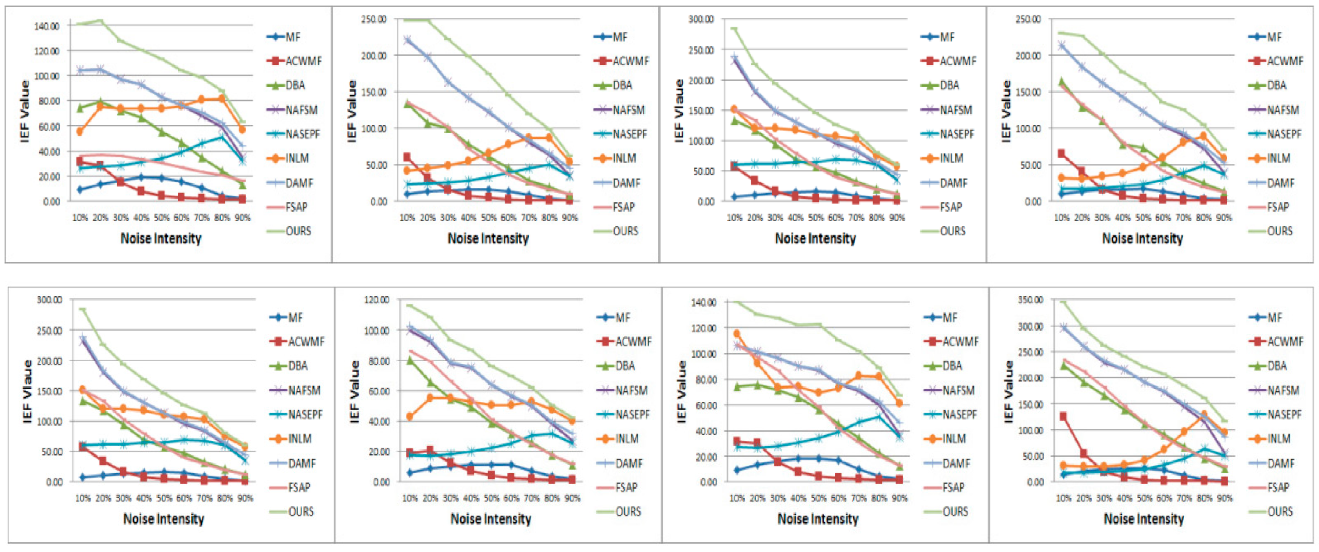
6.4. Objective Quality Analysis

This section presents the visual results obtained by different methods. We evaluated the performance of the proposed method and the methods under comparison via reconstructed images and the corresponding error images, which showed that the error image presented the difference between the original image and the reconstructed image. In the error image, the white point was the error between the de-noised image and the original image. The whiter point denotes the larger difference.
The subjective analysis of the proposed method against the existing methods with different noise intensities were shown in Figure 7, Figure 8, Figure 9 and Figure 10. In these figures, the proposed method was performed in different texture types of images under σ = 60%, 70%, 80%, and 90%.
To explore the visual quality of different methods, we showed the reconstructed images with different noise densities. Figure 7 and Figure 8 show the restoration results of various methods for the test images, which were corrupted by salt and pepper noise with 60% and 70% noise density, respectively. The MF and ACWMF were also found to fail in restoring the corrupted image. In the reconstructions obtained by DBA and NAFSM, many artifacts exist, which make the contours of the estimated images indistinguishable. The DBA, NAFSM, INLM, DAMF, and FSAP can restore the image with better quality. However, the error noise still exists in the reconstructions. Therefore, the results indicated that the proposed method can preserve details better than other methods.
Figure 9 and Figure 10 show the restoration results of different methods for images that were corrupted by heavy salt and pepper noise with 80% and 90% noise density, respectively. In these figures, the first and third rows were the original images and reconstructed images, respectively. The second and fourth rows were the noised image and corresponding error images, respectively. The SM and DWM filters failed to restore images corrupted by the heavy noise. The visual perception of the reconstructions obtained by MDWM filter was bad because some obvious white and black pixels still exist in the restored images.
Figure 7, Figure 8, Figure 9 and Figure 10 show that the proposed method achieved better visual quality. Our proposed method can preserve texture regions or edge regions by adaptively calculating the nonlocal region features and estimate the original pixel value. Thereby, the proposed method reduces reconstruction error as far as possible. Moreover, in the existing methods, undesirable artificial artifacts were inevitably produced in the reconstructed images. As we expected, satisfactory visual effects obtained by our developed algorithm were more natural and have fewer artifacts, especially in high noise intensities.

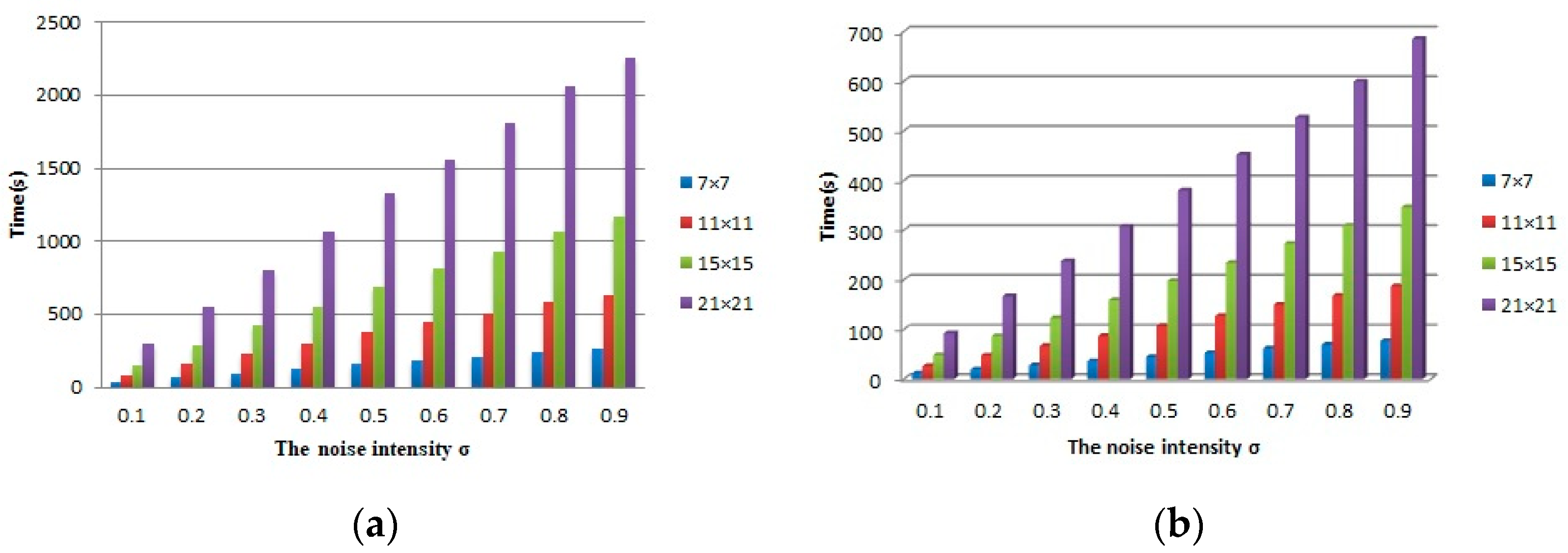
6.5. Effect of Searching Window

In this subsection, we will explore the denoising effect of the proposed method under several searching windows with different size, including 7 × 7, 11 × 11, 15 × 15, and 21 × 21. We take four images as test images, in which two 256 × 256 (i.e., Dog and Zebra images) and two 512 × 512 images (i.e., boat and Man images), and nine noise levels from σ = 10–90% are used to generate synthetic noising images. Table 9 presents the average PSNR and SSIM values of the test images under the contribution of different searching windows. In addition to these two quality metrics, another important aspect is the testing speed. Figure 11 shows the average run times of the proposed method with different searching windows for denoising images with 10 noise levels.
From Figure 11 and Table 9, we can see that the methods based on searching windows with 7 × 7 and 11 × 11 have high speed. With the noise intensity increases, the speed is lower. Compare with the methods based on searching windows with 7 × 7, 11 × 11, 15 × 15, respectively, the method based on 21 × 21 window does not achieve obvious higher PSNR and SSIM values. Although more pixels contribute to the estimation, not all pixels are beneficial to restore the corrupted pixels. Moreover, its speed is fairly slow due to the use of more pixels than other windows. Take the 256 × 256 images for example, the average running time, PSNR and SSIM values achieved corresponding to σ = 10% and searching windows with 7 × 7, 11 × 11, 15 × 15, 21 × 21 respectively are shown in the following: method based on 7 × 7 window (10 s, 30.26 db, 0.9681), method based on 11 × 11 window (26 s, 29.27 db, 0.9682), method based on 15 × 15 window (48 s, 30.17 db, 0.9686), method based on 21 × 12 window (92 s, 30.36 db, 0.9684). In the case of σ = 90%, the average running time, PSNR and SSIM values achieved by different methods are shown in the following: method based on 7 × 7 window (77 s, 18.64 db, 0.5687), method based on 11 × 11 window (187 s, 18.68 db, 0.5557), method based on 15 × 15 window (346 s, 18.67 db, 0.5489), method based on 21 × 12 window (684 s, 18.66 db, 0.5440). Therefore, the searching window with 11 × 11 gains the best performance among all the cases when all of these factors are considered together.

7. Conclusions

This paper presented an adaptive nonlocal bilateral filter for salt and pepper noise removal. First, the NAFSM filter was introduced to distinguish the noisy and noise-free pixels and then conduct preliminary filtering on the noisy pixels. Second, an adaptive norm with scale parameters calculated based on local feature was designed to measure the intensity difference between image patches. Finally, the nonlocal thought, the bilateral thought, and the adaptive norm were combined. Then an adaptive nonlocal bilateral filter was designed to suppress the Gaussian–Laplacian mixture noise and further improve the reconstruction quality.
In Section 6, we demonstrate the benefit of our proposed method on the salt and pepper noise removal problem. We first conduct experiments to verify the effectiveness of the adaptive norm adopted in the novel bilateral filter. We have observed that adaptive norm gives comparable or better results compared to the L1 norm and L2 norm. Then, we demonstrate that the proposed bilateral filter could effectively weaken the median-type filter errors. Especially for the high noisy intensity (σ = 90%), the proposed bilateral filter can obtain satisfactory results. We demonstrate the capability of our proposed method with some state-of-art methods with different noise intensities from σ = 10% to σ = 90%. Numerical results illustrated that the proposed method outperformed the state-of-art methods with better visual quality and higher quality metric values. It indicates the effectiveness of our method to use a two-step framework based on the novel-designed adaptive nonlocal bilateral (ANB) filter. Finally, in order to explore the denoising effect of the proposed method under different searching windows, we also compare the denoising results with different window sizes, including 7 × 7, 11 × 11, 15 × 15, and 21 × 21. Comprehensively considering the running time, PSNR and SSIM values, the searching window with 11 × 11 is proven to be a better choice.

Author Contributions

Data curation, H.L.; Formal analysis, S.Z.; Funding acquisition, H.L., N.L., and S.Z.; Methodology, H.L. and S.Z.; Writing—original draft, H.L.; Writing—review & editing, H.L., N.L., and S.Z. All authors have read and agreed to the published version of the manuscript.

Funding

National Natural Science Foundation of China: 61802213; Shandong Provincial Natural Science Found: ZR2020MF039; National Key Research and Development Project: 2019YFB1404701; The Major Science and Technology Innovation Projects of Key R&D Programs of Shandong Province in 2019 (Development and Industrialization of Pathological Artifificial Intelligence Application Software): 2019JZZY010108; Qilu University of Technology (Shandong Academy of Sciences) Young doctor Cooperation Fund Project: 2019BSHZ009.

Institutional Review Board Statement

Not applicable.

Conflicts of Interest

The authors declare no conflict of interest.

References

  1. Yuan, G.; Ghanem, B. TV: A Sparse Optimization Method for Impulse Noise Image Restoration. IEEE Trans. Pattern Anal. Mach. Intell. 2019, 41, 352–364. [Google Scholar] [CrossRef] [Green Version]
  2. Jin, L.; Zhu, Z.; Song, E.; Xu, X. An Effective Vector Filter for Impulse Noise Reduction Based on Adaptive Quaternion Color Distance Mechanism. Signal Process. 2019, 155, 334–345. [Google Scholar] [CrossRef]
  3. Veerakumar, T.; Subudhi, B.N.; Esakkirajan, S.; Pradhan, P.K. Iterative Adaptive Unsymmetric Trimmed Shock Filter for High-density Salt-and-pepper Noise Removal. Circuits Syst. Signal Process. 2019, 38, 2630–2652. [Google Scholar] [CrossRef]
  4. Fu, B.; Zhao, X.; Song, C.; Li, X.; Wang, X. A Salt and Pepper Noise Image Denoising Method Based on the Generative Classification. Multimed. Tools Appl. 2019, 78, 12043–12053. [Google Scholar] [CrossRef] [Green Version]
  5. Chen, F.; Huang, M.; Ma, Z.; Li, Y.; Huang, Q. An Iterative Weighted-Mean Filter for Removal of High-Density Salt-and-Pepper Noise. Symmetry 2020, 12, 1990. [Google Scholar] [CrossRef]
  6. Zeng, X.; Yang, L. A Robust Multiframe Super-resolution Algorithm Based on Half-quadratic Estimation with Modified BTV Regularization. Digit. Signal Process. Rev. J. 2013, 23, 98–109. [Google Scholar] [CrossRef]
  7. Zhang, X.-M.; Kang, Q.; Cheng, J.-F.; Wang, X. Adaptive Four-dot Median Filter for Removing 1–99% Densities of Salt and-pepper Noise in Images. J. Inf. Technol. Res. 2018, 11, 47–61. [Google Scholar] [CrossRef]
  8. Rhee, K.H. Improvement Feature Vector: Autoregressive Model of Median Filter Error. IEEE Access 2019, 7, 77524–77540. [Google Scholar] [CrossRef]
  9. Storath, M.; Weinmann, A. Fast Median Filtering for Phase or Orientation Data. IEEE Trans. Pattern Anal. Mach. Intell. 2018, 40, 639–652. [Google Scholar] [CrossRef]
  10. Gao, H.; Hu, M.; Gao, T.; Cheng, R. Robust Detection of Median Filtering Based on Combined Features of Difference Image. Signal Process. Image Commun. 2019, 72, 126–133. [Google Scholar] [CrossRef]
  11. Zhang, Z.; Han, D.; Dezert, J.; Yang, Y. A New Adaptive Switching Median Filter for Impulse Noise Reduction with Pre-detection Based on Evidential Reasoning. Signal Process. 2018, 147, 173–189. [Google Scholar] [CrossRef]
  12. Zhu, Z.; Jin, L.; Song, E.; Hung, C.-C. Quaternion Switching Vector Median Filter Based on Local Reachability Density. IEEE Signal Process. Lett. 2018, 25, 843–847. [Google Scholar] [CrossRef]
  13. Chanu, P.R.; Singh, K.M. A Two-stage Switching Vector Median Filter Based on Quaternion for Removing Impulse Noise in Color Images. Multimed. Tools Appl. 2019, 78, 15375–15401. [Google Scholar] [CrossRef]
  14. Sanaee, P.; Moallem, P.; Razzazi, F. An Interpolation Filter Based on Natural Neighbor Galerkin Method for Salt and Pepper Noise Restoration with Adaptive Size Local Filtering Window. Signal Image Video Process. 2019, 13, 895–903. [Google Scholar] [CrossRef]
  15. Varatharajan, R.; Vasanth, K.; Gunasekaran, M.; Priyan, M.; Gao, X.Z. An Adaptive Decision Based Kriging Interpolation Algorithm for the Removal of High Density Salt and Pepper Noise in Images. Comput. Electr. Eng. 2018, 70, 447–461. [Google Scholar] [CrossRef]
  16. Toh, K.K.V.; Isa, N.A.M. Noise Adaptive Fuzzy Switching Median Filter for Salt-and-pepper Noise Reduction. IEEE Signal Process. Lett. 2010, 17, 281–284. [Google Scholar] [CrossRef] [Green Version]
  17. Ibrahim, H.; Kong, N.S.P.; Foo, T.F. Simple Adaptive Median Filter for the Removal of Impulse Noise from Highly Corrupted Images. IEEE Trans. Consum. Electron. 2008, 54, 1920–1927. [Google Scholar] [CrossRef]
  18. Toh, K.K.V.; Ibrahim, H.; Mahyuddin, M.N. Salt-and-pepper Noise Detection and Reduction Using Fuzzy Switching Median Filter. IEEE Trans. Consum. Electron. 2008, 54, 1956–1961. [Google Scholar] [CrossRef]
  19. Wang, Y.; Wang, J.; Song, X.; Han, L. An Efficient Adaptive Fuzzy Switching Weighted Mean Filter for Salt-and-pepper Noise Removal. IEEE Signal Process. Lett. 2016, 23, 1582–1586. [Google Scholar] [CrossRef]
  20. Kumar, S.V.; Nagaraju, C. T2FCS Filter: Type 2 Fuzzy and Cuckoo Search-based Filter Design for Image Restoration. J. Vis. Commun. Image Represent. 2019, 58, 619–641. [Google Scholar] [CrossRef]
  21. González-Hidalgo, M.; Massanet, S.; Mir, A.; Ruiz-Aguilera, D. Improving Salt and Pepper Noise Removal Using a Fuzzy Mathematical Morphology-based Filter. Appl. Soft Comput. J. 2018, 63, 167–180. [Google Scholar] [CrossRef]
  22. Khosravy, M.; Gupta, N.; Marina, N.; Sethi, I.K.; Asharif, M.R. Morphological Filters: An Inspiration from Natural Geometrical Erosion and Dilation. In Nature Inspired Compututer Optimization; Springer: Cham, Switzerland, 2017; pp. 349–379. [Google Scholar]
  23. Sedaaghi, M.H.; Daj, R.; Khosravi, M. Mediated Morphological Filters. In Proceedings of the 2001 International Conference on Image Processing, Thessaloniki, Greece, 7–10 October 2001; 2001; pp. 692–695. [Google Scholar]
  24. Khosravi, M.; Sedaaghi, M.H. Impulsive Noise Suppression of Electrocardiogram Signals with Mediated Morphological Filters. In Proceedings of the 11th Iranian Conference on Biomedical Engineering, Teheran, Iran, 18 February 2004. [Google Scholar]
  25. Khosravy, M.; Asharif, M.R.; Sedaaghi, M.H. Morphological Adult and Fetal ECG Preprocessing: Employing Mediated Morphology. IEICE Med. Imaging 2007, 107, 363–369. [Google Scholar]
  26. Khosravy, M.; Asharif, M.R.; Sedaaghi, M.H. Medical Image Noise Suppression: Using Mediated Morphology. IEICE Tech. Rep. 2008, 107, 265–270. [Google Scholar]
  27. Mafi, M.; Rajaei, H.; Cabrerizo, M.; Malek, A. A Robust Edge Detection Approach in the Presence of High Impulse Noise Intensity through Switching Adaptive Median and Fixed Weighted Mean Filtering. IEEE Trans. Image Process. 2018, 27, 5475–5490. [Google Scholar] [CrossRef]
  28. Balasubramanian, S.; Kalishwaran, S.; Muthuraj, R.; Ebenezer, D.; Jayaraj, V. An Efficient Non-linear Cascade Filtering Algorithm for Removal of High Density Salt and Pepper Noise in Image and Video Sequence. In Proceedings of the IEEE International Conference Control, Automation, Communication and Energy Conservation (INCACEC), Perundurai, Erode, India, 4–6 June 2009; pp. 1–6. [Google Scholar]
  29. Raza, M.T.; Sawant, S. High Density Salt and Pepper Noise Removal through Decision Based Partial Trimmed Global Mean Filter. In Proceedings of the IEEE International Conference Engineering (NUiCONE), Ahmedabad, Gujarat, India, 6–8 December 2012; pp. 1–5. [Google Scholar]
  30. Esakkirajan, S.; Veerakumar, T.; Subramanyam, A.N.; Chand, C.H.P. Removal of High Density Salt and Pepper Noise through Modified Decision Based Unsymmetrical Trimmed Median Filter. IEEE Signal Process. Lett. 2011, 18, 287–290. [Google Scholar] [CrossRef]
  31. Wang, X.; Shen, S.; Shi, G.; Xu, Y.; Zhang, P. Iterative Non-local Means Filter for Salt and Pepper Noise Removal. J. Vis. Commun. Image Represent. 2016, 38, 440–450. [Google Scholar] [CrossRef]
  32. Veerakumar, T.; Subudhi, B.N.; Esakkirajan, S. Empirical Mode Decomposition and Adaptive Bilateral Filter Approach for Impulse Noise Removal. Expert Syst. Appl. 2019, 121, 18–27. [Google Scholar] [CrossRef]
  33. Mafi, M.; Martin, H.; Cabrerizo, M.; Andrian, J.; Barreto, A.; Adjouadi, M. A Comprehensive Survey on Impulse and Gaussian Denoising Filters for Digital Images. Signal Process. 2019, 157, 236–260. [Google Scholar] [CrossRef]
  34. Nair, P.; Chaudhury, K.N. Fast High-dimensional Bilateral and Nonlocal Means Filtering. IEEE Trans. Image Process. 2019, 28, 1470–1481. [Google Scholar] [CrossRef] [PubMed]
  35. Karthikeyan, P.; Vasuki, S. Efficient Decision Based Algorithm for the Removal of High Density Salt and Pepper Noise in Images. J. Commun. Technol. Electron. 2016, 61, 963–970. [Google Scholar] [CrossRef]
  36. Wang, Z.; Bovik, A.C.; Sheikh, H.R.; Simoncelli, E.P. Image Quality Assessment: From Error Visibility to Structural Similarity. IEEE Trans. Image Process. 2004, 13, 600–612. [Google Scholar] [CrossRef] [PubMed] [Green Version]
  37. Chen, T.; Wu, H.R. Adaptive Impulse Detection Using Center Weighted Median Filters. IEEE Signal Process. Lett. 2001, 8, 1–3. [Google Scholar] [CrossRef]
  38. Jiang, D.-S.; Li, X.-B.; Wang, Z.-L.; Liu, C. An Efficient Edge-preserving Approach Based on Adaptive Fuzzy Switching Median Filter. In Proceedings of the 2011 International Conference on Quality, Reliability, Risk, Maintenance, and Safety Engineering, Xi’an, China, 17–19 June 2011; pp. 952–955. [Google Scholar]
  39. Erkan, U.; Gökrem, L.; Enginoğlu, S. Different Applied Median Filter in Salt and Pepper Noise. Comput. Electr. Eng. 2018, 70, 789–798. [Google Scholar] [CrossRef]
  40. Srinivasan, K.S.; Ebenezer, D. A New Fast and Efficient Decision-based Algorithm for Removal of High-density Impulse Noises. IEEE Signal Process. Lett. 2007, 14, 189–192. [Google Scholar] [CrossRef]
  41. Singh, V.; Dev, R.; Dhar, N.K.; Agrawal, P.; Verma, N.K. Adaptive Type-2 Fuzzy Approach for Filtering Salt and Pepper Noise in Grayscale Images. IEEE Trans. Fuzzy Syst. 2018, 26, 3170–3176. [Google Scholar] [CrossRef]
Figure 1. Error image and the corresponding histogram. (a) Error image between I and Iori for image “Lena”; (b) histogram of (a); (c) error image between Iori and I ^ m f for the image “Lena”; (d) histograms of the error image for 10 images.
Symmetry 13 00515 g001
Figure 2. Curve of ψ ( t ) with different a values.
Symmetry 13 00515 g002
Figure 3. Simple example.
Symmetry 13 00515 g003
Figure 4. Twelve test images. (a) Cameraman; (b)Barbara; (c) Couple; (d) Dog; (e) Lena; (f) Man-made; (g) Pepper; (h) Zebra; (i)Baboon; (j) Street; (k) Boat; (l) Man.
Symmetry 13 00515 g004
Figure 5. Comparisons of the pre- and post-processed images. In each line, the left part is the original image, the middle part is the zoomed details. The pre-processed marked “1”, the post-processed marked “2”. The right part is the corresponding error images, the first one is pre-processed error, the second one is post-processed error.
Symmetry 13 00515 g005
Figure 6. Comparison of different methods. From top left to right down: the curves of IEF vs. noise intensity achieved for the images Baboon, Pepper, Man-made, Lena, Couple, Cameraman, Barbara, Street.
Symmetry 13 00515 g006
Figure 7. Results of different algorithms for Barbara image with 60% noise intensity. The subfigures in rounded rectangle are corresponding to original image, MF, ACWMF, DBA, NAFSM, NASEPF, INLM, DAMF, FSAP, and our proposed method, respectively.
Symmetry 13 00515 g007
Figure 8. Results of different algorithms for Cameraman image with 70% noise intensity. The subfigures in the first line from left to right are corresponding to original image, MF, ACWMF, DBA, and NAFSM, respectively. The subfigures in the third line from left to right are NASEPF, INLM, DAMF, FSAP, and our proposed method, respectively.
Symmetry 13 00515 g008
Figure 9. Results of different algorithms for Man-made image with 80% noise intensity. The first and third lines are original image, MF, ACWMF, DBA, NAFSM, NASEPF, INLM, DAMF, FSAP, and our proposed method. The second and fourth lines are noise image and corresponding error images.
Symmetry 13 00515 g009
Figure 10. Results of different algorithms for Lena image with 90% noise intensity. The first and third lines are original image, MF, ACWMF, DBA, NAFSM, NASEPF, INLM, DAMF, FSAP, and our proposed method. The second and fourth lines are noise image and corresponding error images.
Symmetry 13 00515 g010
Figure 11. Average running time comparison based on different search window sizes for (a) 512 × 512 images and (b) 256 × 256 images. The provided values of search window size are 7 × 7, 11 × 11, 15 × 15, and 21 × 21.
Symmetry 13 00515 g011
Table 1. PSNR comparison for our proposed method, L1-based method, and L2-based method with the noise intensity varied from 10% to 90%.
ImageMethodσ = 10%σ = 20%σ = 30%σ = 40%σ = 50%σ = 60%σ = 70%σ = 80%σ = 90%
BarbaraOURS36.2832.9331.0729.6028.6427.4226.3825.2123.47
L1-based36.1932.6030.7729.3128.4027.2426.2224.9923.40
L2-based36.7833.3830.8729.2127.9526.5325.4624.2322.34
Man-madeOURS43.6138.8335.9633.1331.0529.3327.4425.7422.39
L1-based42.8038.6635.5432.7731.5429.1926.2424.6522.23
L2-based42.3438.4835.1632.2830.5928.2226.9924.4621.30
Table 2. SSIM comparison for our proposed method, L1-based method, and L2-based method with the noise intensity varied from 10% to 90%.
ImageMethodσ = 10% σ = 20%σ = 30%σ = 40%σ = 50%σ = 60%σ = 70%σ = 80%σ = 90%
BarbaraOURS0.98370.96430.94310.91790.89550.86410.82500.77660.6927
L1-based0.98290.96170.93920.91260.88980.85790.81780.77180.6901
L2-based0.98630.96970.94480.91800.88800.84960.80790.75190.6639
Man-madeOURS0.99820.99450.98920.97950.96820.95290.92980.90180.8285
L1-based0.99780.99430.98860.97960.97380.95600.90690.87110.8113
L2-based0.99800.99520.99000.98200.97310.95490.94110.90010.8229
Table 3. IEF comparison for our proposed method, L1-based method, and L2-based method with the noise intensity varied from 10% to 90%.
ImageMethodσ = 10% σ = 20%σ = 30%σ = 40%σ = 50%σ = 60%σ = 70%σ = 80%σ = 90%
BarbaraOURS140.416130.547127.952122.382122.607110.510101.75288.89567.242
L1-based139.339121.283120.390114.770116.538106.41598.44385.11566.178
L2-based160.801146.468123.910113.409105.97191.061583.41871.69452.399
Man-madeOURS631.958582.068443.847341.676299.842208.344131.92197.47558.901
L1-based753.249562.153421.249295.480281.036192.859113.37489.55257.791
L2-based678.310542.347388.393265.755226.931154.95136.95987.18847.458
Table 4. PSNR Comparisons between pre- and post-processed images.
ImageMethodσ = 10%σ = 20%σ = 30%σ = 40%σ = 50%σ = 60%σ = 70%σ = 80%σ = 90%
CouplePre-processed38.1034.0831.4829.6828.0726.5325.2723.5220.48
Post-processed39.1035.2932.7330.8629.2127.7926.6425.0622.86
PepperPre-processed37.5433.8731.5029.6128.0526.4424.7823.1420.14
Post-processed37.7635.0132.9131.1529.6228.0126.5425.1322.65
StreetPre-rocessed39.3635.8233.4731.9530.5029.2427.8026.2522.57
Post-rocessed40.2436.4034.0732.4831.1430.0828.9027.7625.84
Table 5. SSIM Comparisons between pre- and post-processed images.
ImageMethodσ = 10%σ = 20%σ = 30%σ = 40%σ = 50%σ = 60%σ = 70%σ = 80%σ = 90%
CouplePre-processed0.98590.97060.95000.92800.90260.86620.82690.76260.6148
Post-processed0.98930.97640.95800.93680.91250.88030.84760.77890.6973
PepperPre-processed0.98710.97070.95470.93000.90520.87270.83100.77350.6456
Post-processed0.98830.97490.96170.94100.92210.89660.86870.83000.7590
StreetPre-processed0.98710.97070.95470.93000.90520.87270.83100.77350.6456
Post-processed0.98830.97490.96170.94100.92210.89660.86870.83000.7590
Table 6. IEF Comparisons between pre- and post-processed images.
ImageMethodσ = 10%σ = 20%σ = 30%σ = 40%σ = 50%σ = 60%σ = 70%σ = 80%σ = 90%
CouplePre-processed232.16180.32148.58130.69112.8695.4383.9862.3535.61
Post-processed284.77226.29194.08168.83145.19126.20113.8280.4060.58
PepperPre-processed221.37197.51163.91141.82122.67102.0681.1763.2035.82
Post-processed248.20248.25222.90199.28174.44145.03120.4598.7163.11
StreetPre-processed295.41260.04229.59215.14191.47172.26144.31115.0355.76
Post-processed345.85293.34261.28241.07220.54207.64184.61161.84117.33
Table 7. Comparison of PSNR values for test images under different noise intensities.
ImageMethodσ = 10%σ = 20%σ = 30%σ = 40%σ = 50%σ = 60%σ = 70%σ = 80%σ = 90%
BarbaraMF24.1322.7421.8821.1720.2819.1816.1911.887.69
ACWMF29.7926.6021.9517.8414.2111.539.177.415.83
DBA33.5630.6928.6827.0725.4523.7221.8919.5416.50
NAFSM34.9731.7829.7828.2127.1025.7724.7323.4420.82
NASEPF29.2826.1424.5623.6923.1722.8922.9422.7220.55
INLM35.4131.4728.7027.4826.2325.6725.5124.8623.07
DAMF34.9731.7829.7828.2127.1225.8024.8223.6421.79
FSAP35.0431.6429.3527.2625.4023.2321.2018.8716.49
OURS36.2832.9331.0729.6028.6427.4226.3825.2123.47
BaboonMF19.5819.3218.9818.6518.2617.3415.2711.317.48
ACWMF25.7623.4520.1616.8113.7511.149.027.245.80
DBA28.0225.9624.2422.8421.5920.2419.0417.7416.15
NAFSM30.8727.8025.9024.3523.0521.8820.7219.4917.69
NASEPF26.5623.6222.0321.0120.3619.9419.5719.0517.55
INLM28.9326.7925.0623.5622.4921.7321.0820.3819.20
DAMF30.8727.8025.9024.3523.0521.8920.7519.5818.15
FSAP30.3527.4525.6024.0322.6221.3720.1318.9717.49
OURS31.2328.0426.0824.5323.3322.3521.4120.4919.35
CameramanMF21.9521.1020.1119.1818.4317.5315.1711.427.58
ACWMF27.7625.2421.3117.6314.3811.609.557.596.09
DBA34.1730.4027.8626.0424.1622.4420.9718.7416.34
NAFSM35.0131.7329.2427.6926.1224.7523.5921.8219.73
NASEPF27.7024.6923.1122.1621.6821.4321.5621.0119.48
INLM31.5129.6627.8526.3125.2324.4223.9422.8621.54
DAMF35.1331.8029.2727.7126.1324.7823.6721.9420.46
FSAP34.4231.1428.5826.3524.2522.4520.6918.6716.43
OURS37.7132.6230.0728.4926.9325.7424.6223.0921.78
CoupleMF22.7921.7521.0620.2419.6618.4515.4811.527.56
ACWMF32.1026.9822.1517.6514.2011.298.907.155.69
DBA35.8432.3429.6827.1125.3823.6421.3419.2216.13
NAFSM38.1034.0831.4829.6828.0726.5325.2723.5220.48
NASEPF32.3429.4527.7326.6525.7325.1824.4023.4120.49
INLM36.2832.3730.6229.2928.0227.0726.1824.4122.66
DAMF38.2234.1431.5129.7028.0926.6525.3223.8121.49
FSAP36.2732.8029.9227.5325.1922.8020.8618.5915.87
OURS39.1035.2932.7330.8629.2127.7926.6425.0622.86
LenaMF25.0023.3922.3221.1520.4918.8116.2612.118.20
ACWMF33.4528.2922.5318.2614.7911.949.687.766.35
DBA37.5433.3430.9628.2427.0224.8922.6420.3317.48
NAFSM38.5434.7332.4630.6629.1027.5626.3124.7121.55
NASEPF27.9924.8423.4022.4722.1322.1722.7223.0321.25
INLM30.4327.2425.8525.0925.0725.3025.9025.6823.39
DAMF38.5434.7332.4630.6629.1127.5826.4624.9522.82
FSAP37.2533.3730.8428.2326.0823.6221.6219.2717.00
OURS39.2535.7333.4631.6330.3028.7627.7726.3624.15
PeppersMF23.8622.2621.0819.9219.1817.8414.8010.956.90
ACWMF31.9226.1121.5816.9113.9310.878.566.805.32
DBA35.4931.3829.5127.2125.2523.1520.5418.5214.67
NAFSM37.5433.8731.5029.6128.0526.4424.7823.1420.14
NASEPF28.1025.1223.7322.7522.4222.3222.2922.1919.96
INLM30.4927.6726.4225.6625.4925.3825.1424.5921.97
DAMF37.5533.8931.5129.6228.0726.4524.9323.3621.17
FSAP35.4331.7929.4726.7724.5222.1919.6817.3114.79
OURS37.7635.0132.9131.1529.6228.0126.5425.1322.65
StreetMF26.1224.9423.6422.7321.8820.4517.0112.067.60
ACWMF35.7429.0422.7718.0214.4311.469.197.365.82
DBA38.2634.6132.1930.2028.3326.6224.6422.3419.47
NAFSM39.3635.8233.4731.9530.5029.2427.8026.2522.57
NASEPF27.3424.4222.8822.1121.8422.1222.8623.7422.13
INLM29.6726.6224.8824.0823.9824.8926.1226.8224.88
DAMF39.3835.8333.5131.9630.5129.2927.9326.5824.42
FSAP38.3634.9532.4730.2728.2326.2924.3222.3619.87
OURS40.2436.4034.0732.4831.1430.0828.9027.7625.84
Man-madeMF23.5920.5718.5117.2116.3015.0213.1010.196.47
ACWMF33.0426.9321.6417.3213.9110.748.636.815.22
DBA37.8133.0230.4027.4324.6522.7520.0917.5914.38
NAFSM39.2935.2632.8330.5428.8927.3525.4023.6919.63
NASEPF18.6915.7614.2413.4713.3513.8315.0116.7717.98
INLM21.4318.2717.1016.9917.6318.8320.8222.6021.48
DAMF40.7435.9133.1930.7228.9827.4425.4423.9520.72
FSAP37.3533.2630.5927.8624.9823.1120.5618.1315.41
OURS43.6138.8335.9633.1331.0529.3327.4425.7422.39
Table 8. Comparison of SSIM values for test images under different noise intensities.
ImageMethodσ = 10%σ = 20%σ = 30%σ = 40%σ = 50%σ = 60%σ = 70%σ = 80%σ = 90%
BarbaraMF0.70480.69690.68520.67490.64710.60840.44660.20350.0466
ACWMF0.94940.89180.73730.50420.29470.15130.07850.03770.0155
DBA0.97690.95070.91740.87970.83190.77290.68640.56780.3945
NAFSM0.97900.95620.92880.89780.86590.82430.77810.71440.5882
NASEPF0.88770.82800.78830.75390.72240.69460.66650.63790.5625
INLM0.97010.93190.88370.85080.81840.79690.77940.75230.6743
DAMF0.97900.95620.92880.89780.86620.82510.78090.72070.6285
FSAP0.97980.95780.92650.88360.82890.74840.64330.50070.3509
OURS0.98340.96410.94270.91740.89490.86330.82420.77570.6898
BaboonMF0.38420.38130.37770.37260.36300.33360.25450.10920.0253
ACWMF0.91890.85780.71910.52110.31620.17060.08570.04120.0188
DBA0.96730.92870.88020.82340.75360.66810.56760.45000.3101
NAFSM0.97040.93730.89890.85570.80310.74280.66880.57450.4240
NASEPF0.86330.79040.73420.68670.63880.59330.54620.49390.3964
INLM0.91410.87850.83060.77590.72240.67330.62250.56180.4605
DAMF0.97040.93730.89890.85570.80320.74320.67000.57890.4463
FSAP0.96830.93450.89290.84070.77000.68680.58090.46320.3315
OURS0.97110.93670.89560.84900.79490.73620.66660.58570.4724
CameramanMF0.72560.72060.71200.69880.67880.63580.48420.18390.0360
ACWMF0.93980.87740.71220.47720.26260.13230.07900.03980.0207
DBA0.98400.96450.93730.90750.86760.81400.76490.67530.5723
NAFSM0.97960.96290.94220.92280.89570.86360.82320.76330.6456
NASEPF0.74350.66410.62210.59280.56970.55010.54310.54080.5597
INLM0.87520.85140.80540.76270.73950.73150.74620.74500.7125
DAMF0.98620.97050.94930.92770.89980.86730.83000.77270.7039
FSAP0.98440.96680.94230.91070.86710.80890.74110.64660.5256
OURS0.98700.97170.95130.92950.90350.87460.84230.79330.7362
CoupleMF0.69410.68620.67580.65680.63650.58530.42750.20180.0521
ACWMF0.96330.90220.74930.53300.32770.16940.08390.04200.0208
DBA0.98610.96700.93780.89960.85680.78930.70240.59020.4184
NAFSM0.98590.97060.95000.92800.90260.86620.82690.76260.6148
NASEPF0.93970.90270.86970.84540.81920.79420.76520.72850.6169
INLM0.97640.95000.92720.90430.87900.85140.82610.76160.6809
DAMF0.98870.97400.95320.93110.90470.86860.82890.76960.6583
FSAP0.98560.96860.94150.90230.84430.75880.65100.51560.3524
OURS0.98930.97640.95800.93680.91250.88030.84760.77890.6973
LenaMF0.76510.75650.74800.73320.70920.65140.47680.19220.0400
ACWMF0.97330.91720.74770.50510.27080.14110.06910.03650.0139
DBA0.98560.96530.94160.90760.86920.81180.73260.62720.4832
NAFSM0.98720.97160.95400.93140.90700.87280.83010.77630.6457
NASEPF0.83100.76040.72020.68870.66890.65040.64370.64180.6035
INLM0.88710.84410.81830.79260.78170.77770.78520.78340.7247
DAMF0.98720.97160.95400.93140.90700.87340.83460.78480.6918
FSAP0.98570.96770.94280.90390.85010.76760.66550.53190.3946
OURS0.98870.97470.95880.93810.91760.88980.85960.82050.7461
PeppersMF0.78810.77650.76680.74690.72370.66740.47880.22340.0546
ACWMF0.96940.89450.74530.49670.31050.16090.07960.04170.0220
DBA0.98560.96330.94250.90580.86460.80640.71340.61500.4374
NAFSM0.98710.97070.95470.93000.90520.87270.83100.77350.6456
NASEPF0.87260.80780.77590.74300.72190.70320.68810.67970.6231
INLM0.91820.87990.86090.83610.82520.81940.81620.80690.7411
DAMF0.98740.97120.95530.93060.90610.87330.83470.78040.6917
FSAP0.98460.96500.94220.90240.84980.77700.67300.54640.3925
OURS0.98830.97490.96170.94100.92210.89660.86870.83000.7590
StreetMF0.67350.66830.65920.64930.63030.58770.43150.17960.0327
ACWMF0.97120.89910.72870.47860.26350.12040.05710.02660.0112
DBA0.98180.95810.92840.88990.84290.78310.69880.59210.4433
NAFSM0.98370.96450.94190.91600.88550.85040.80240.73790.5966
NASEPF0.87130.82550.79310.76440.73750.71180.68200.64710.5626
INLM0.90240.86510.83640.80660.78180.76250.74560.72910.6696
DAMF0.98410.96490.94220.91640.88600.85110.80470.74560.6431
FSAP0.98270.96280.93690.90140.85500.79400.71330.61740.4985
OURS0.98580.96630.94350.91730.88880.85810.81900.77260.6944
Man-madeMF0.88450.87600.86150.84180.81890.74230.57030.30170.0752
ACWMF0.93380.85290.70480.50120.32180.17280.09890.05320.0222
DBA0.99480.98500.97260.94950.91810.87440.80170.71750.5581
NAFSM0.97270.96250.95640.94830.94380.93060.90800.87210.7508
NASEPF0.45270.38860.35750.33810.32940.32850.33860.36790.4477
INLM0.55640.47120.44170.42810.43450.45990.52990.63270.7354
DAMF0.99680.99130.98440.97230.96060.94350.91620.88470.8002
FSAP0.99390.98510.97240.94710.90680.86150.77890.65580.4802
OURS0.99820.99450.98920.97950.96820.95290.92980.90180.8285
Table 9. Comparison of average PSNR/SSIM values for the test images with four search window sizes (SWS) and nine noise intensities.
Image SizeSWSStandardσ = 10%σ = 20%σ = 30%σ = 40%σ = 50%σ = 60%σ = 70%σ = 80%σ = 90%
256 × 256 7 × 7 PSNR 30.26 27.25 26.86 25.62 24.22 23.10 21.97 20.53 18.64
SSIM 0.9681 0.9481 0.9250 0.8939 0.8567 0.8104 0.7539 0.6820 0.5687
11 × 11 APSNR 29.27 26.90 26.54 25.42 24.19 22.97 21.87 20.45 18.68
SSIM 0.9682 0.9472 0.9227 0.8908 0.8510 0.8023 0.7439 0.6687 0.5557
15 × 15 PSNR 30.17 28.27 26.57 25.5428 24.13 22.54 21.79 20.39 18.67
SSIM 0.9686 0.9484 0.9219 0.8892 0.8482 0.7976 0.7389 0.6625 0.5489
21 × 21 PSNR 30.36 28.19 25.81 25.40 24.05 22.78 21.73 20.35 18.66
SSIM 0.9684 0.9479 0.9207 0.8870 0.8453 0.7945 0.7353 0.6591 0.544
512 × 512 7 × 7 PSNR 36.74 34.52 32.47 31.00 29.66 28.40 27.12 25.83 23.82
SSIM 0.9820 0.9667 0.9462 0.9220 0.8937 0.8608 0.8203 0.7698 0.6020
11 × 11 PSNR 35.62 34.16 32.44 30.78 29.41 28.11 26.85 25.60 23.77
SSIM 0.9818 0.9656 0.9442 0.9178 0.8870 0.8510 0.8077 0.7547 0.6784
15 × 15 PSNR 36.53 34.28 32.33 30.66 29.28 27.93 26.65 25.42 23.67
SSIM 0.9818 0.9654 0.9429 0.9154 0.8835 0.8459 0.8010 0.7472 0.6707
21 × 21 PSNR 36.69 34.48 32.24 30.55 29.15 27.76 26.46 25.23 23.52
SSIM 0.9818 0.9653 0.9419 0.9134 0.8806 0.8416 0.7958 0.7413 0.6648
Publisher’s Note: MDPI stays neutral with regard to jurisdictional claims in published maps and institutional affiliations.

