1. Introduction
The multi-criteria analysis is an effective decision-making tool in choosing an appropriate alternative depending on different quantitative and qualitative criteria. The fuzzy logic has many applications in decision-making by using multi-criteria analysis. The fuzzy based multi-criteria decision making (MCDM) methods enable handling of uncertainty during decision-making process.
The sustainable development in passenger railway transport depends on development of the passenger train planning. The transport plan includes the itineraries, the number of trains by category, and the planning of rolling stock. The determination of the transport plan depends on different quantitative and qualitative criteria affecting the transport process, which in many cases cannot be precisely determined. This is due to the unevenness of passenger flows, which affects the choice of transport services. The main objective for railway transport operators is to determine the suitable transport plan by comparing different alternatives. When evaluating the passenger satisfaction in passenger railway transport, it is necessary to take into account the uncertainty of criteria influencing on transport process.
The hypothesis of this research is that the uncertainty of criteria related to transport process have to be taken into account in the choice of a suitable transport plan in passenger railway transport. The research questions are addressed to the following issues: how the decision maker selects the appropriate alternative in the case of uncertainty considering the decisions obtained by applying optimization methods; how to eliminate subjectivism in decision making; how to increase the adequacy of the results.
The sequential interactive model for urban systems method (SIMUS) is based on linear programming. The experts’ assessment of the criteria is not used. The ranking of alternatives is performed according to multiple objectives and consistent application of linear optimization models for each objective. The SIMUS method allows to decision-making to assess different alternatives in the case of certainty, i.e., according predetermined constant values of criteria. However, for some criteria the exact values may not be known or cannot be determined, i.e., the decision-making is in a state of uncertainty and risk. In this case, it is necessary to use methods that allow several values of the criteria to be set in order to determine the appropriate alternative. The fuzzy multi-criteria methods are suitable for decision making.
The aim of this research is to extend the SIMUS method by elaborating a novel fuzzy multi-criteria method, based on the SIMUS approach and fuzzy linear programming, named fuzzy SIMUS for selecting the appropriate alternative.
The application of novel fuzzy SIMUS approach it this paper is presented in railway transport for selecting the appropriate alternative of transport plan for intercity trains.
The advantages of the novel fuzzy SIMUS method are as follows: it does not use expert assessments to evaluate the criteria and rank the alternatives; it permits to decision-maker to solve problems in the case of uncertainty; it uses fuzzy linear optimization for each objective, which allows to determine the score of each objective; it gives a ranking of the alternatives; the multi-criteria and multi-objective approaches to decision making are combined to increase the adequacy of the results; it also allows the weights of the criteria to be determined if the decision-maker wants to analyse them.
This paper is structured as follows.
Section 2 presents a literature review.
Section 3 presents the material and methods, wherein the proposed novel fuzzy SIMUS methodology is explained in detail.
Section 4 includes the presentation of the results obtained by using the new approach.
2. Literature Review
The different multi-criteria methods in fuzzy environment were applied to study various transport problems. The fuzzy set theory that expresses uncertainties is used together with the multi-criteria methods which permit to get more realistic results.
Some fuzzy multi-criteria methods can only be used to determine the weights of criteria, while others serve for ranking the alternatives by setting the weights of the criteria. Others have solved weights of criteria by applying expert’s assessment and a scale of evaluation, and also ranking the alternatives.
Table 1 summarizes the available fuzzy MCDM approaches in the transport area.
The fuzzy multi-criteria methods can be summarized as follows: pair-wise comparisons [
1,
2,
3,
4,
5,
6,
7,
8,
9]; distance based [
10,
11,
12,
13,
14,
15,
16,
17,
18]; utility based [
19,
20,
21,
22,
23,
24,
25,
26]; outranking [
27,
28]; integration of two or more methods [
29,
30,
31,
32,
33,
34,
35,
36].
The main problems solved in the transport planning area are concerned with railway transport [
4,
17,
26,
28,
31,
35], transport planning [
2,
3,
9,
12,
13,
24], railway infrastructure [
6,
16,
23], public transport [
1,
7,
11,
30,
33], logistics [
5,
10,
20,
21,
25,
27,
32,
33,
36].
It can be seen that the most used approaches for multi-criteria decision making in the case of uncertainty are fuzzy AHP [
1,
2,
3,
4,
5,
6,
7], fizzy TOPSIS [
12,
13,
14,
15], and fuzzy VIKOR [
16,
17,
18] techniques, and also integration with additional multi-criteria methods [
29,
30,
31,
32,
33,
34,
35,
36]. New methods based on AHP have also been developed, such as graphical AHP and fuzzy C-Means, [
37].
There are many papers linking fuzzy with AHP, TOPSIS, PROMETHEE, etc., and all of them followed the same procedure, while this paper is something completely different because it links the power of fuzzy with the advantage of the SIMUS method. Not using weights, it works with optimal values.
The different multi-criteria methods applied in transport research area were analyzed in [
38,
39,
40]. An analysis of fuzzy multi criteria decision making methods were presented in [
41,
42]. The fuzzy multi-criteria methods use subjective and objective approaches. The subjective approaches take into account the expert’s subjective opinion. So, the experts influence of the results and decision-making process too. Many methods rank alternatives based on different mathematical approaches, but they require the weights to be set by the decision maker. The subjectivism decreases if the weights of the criteria are determined by the entropic method, correlation methods, and other mathematical approaches. The objective approach to decision making does not affect the results, but uses mathematical approaches and optimizations to give reliable solutions.
The SIMUS method does not use the subjective approach. SIMUS was developed by Nolberto Munier and was applied in many and diverse projects, [
43,
44,
45]. It uses each criterion as an objective and applied linear programming method to make optimization based on each criterion. There is no need to compute weights for criteria, since the method internally calculates their relative importance and applies it in each iteration.
The SIMUS method was applied to evaluate of railway network performance in countries of the TEN-T Orient-East Med Corridor, [
46]. The new integrated approach to decision making in the case of uncertainty based on the SIMUS method was proposed in [
47]. The SIMUS, AHP, and decision tree methods were applied for planning railway passenger transport. The methodology was tested for the Bulgarian railway network. The uncertainty of passenger flows was studied.
The difference of this study and related researches is based on the elaborated approach. The fuzzy extension of SIMUS method in literature is not presented. This paper deal with the problem of uncertainty in decision making by elaborating a novel fuzzy SIMUS method.
3. Materials and Methods
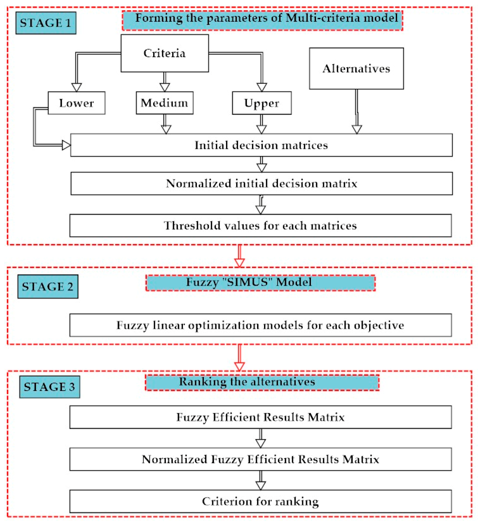
Figure 1 shows the scheme of the methodology of novel fuzzy SIMUS method. The methodology consists tree stages: the first stage includes forming the parameters of a multi-criteria model in the case of uncertainty; in the second stage, the fuzzy SIMUS model for each objective is formed by applying the fuzzy linear programming method. The third stage deals with the ranking of the alternatives.
3.1. Stage 1: Forming the Parameters of Multi-Criteria Model
3.1.1. Step 1. Forming the Initial Decision-Making Matrices
The methodology starts with an initial matrix that has three values, lower (L), medium (M), and upper (U).
For the criteria three values are set: lower, medium and upper. The matrices [
], [
], [
] are formed, as follows, (
is the left-hand side of the inequations):
where:
is the number of criteria (objectives);
is the number of alternatives;
—lower value;
m—medium value;
u—upper value;
are the lower value for criterion
and alternative
j;
are the medium value for criterion
and alternative
j;
are the upper value for criterion
and alternative
j.
The three values for each criterion are averaged for each alternative. With this, the original matrix is reduced to a simple one with averaged values as performance values.
The average value
for each criterion and each alternative is determined as follows:
The average value for each criterion and each alternative could also be determined by the project evaluation and review technique (PERT) method as follows:
So, the average decision matrix is determined [.
3.1.2. Determination of the Normalized Matrices
The normalization could be made by different methods, for example sum of the row, maximum element or other. This step includes normalization of the initial decision-making matrices [], [], [], and also the average matrix []. The normalized matrix [] is determined for the decision matrix on the upper values of the criteria []. The normalized matrix [] for decision-making on the lower values of the criteria is formed. The normalized matrix of the average decision matrix is determined [].
The elements of the normalized matrices are presented as follows:
where:
are the normalized lower value for criterion
and alternative
j;
are the normalized medium value for criterion
and alternative
j;
are the normalized upper value for criterion
and alternative
j;
are the normalized average value for criterion
and alternative
j.
3.1.3. Step 3. Determination of the Threshold Values of the Criteria (), (RHS Is Right Hand Side of Inequations)
For this purpose, the normalized matrices [] and [] are used. The and for these matrices are respectively defined. The threshold values are determined separately of each row of the matrices [] and []. In the case of maximum of objective function, the value of RHS is equal of maximum normalized value of the row. The value of is equal of minimum normalized value of the row when the objective function is of minimum.
3.2. Stage 2 Forming the Fuzzy SIMUS Model for Each Objective
3.2.1. Step 1. Solving SIMUS Procedure for Upper and Lower Initial Decision-Making Matrices
The method works with the optimal lower and upper values. In so doing, the scores for each alternative for upper and lower values are obtained. Then, it becomes be possible to analyze how the rank is altered.
In this step the classical SMUS method is applied for [] and [] decision-making matrices and get for each objective the optimal value for lower and upper matrices. The successive linear optimization models are compiled for each criterion separately. The values of objective function per criterion are determined by solving SIMUS method for [] matrix. The value of objective function per criterion is determined by solving SIMUS method for [] matrix. Both and are used in the next step in fuzzy liner optimization models.
For example, for objective 1, the linear optimization model for lower values of criteria is presented as follows:
Restrictive conditions:
where:
is the score of alternative j when the first criterion is used as an objective.
When the objective function is of maximum, the operator is . In the case of minimum of the objective function, the operator is .
The linear optimization model for upper values of criteria is formed in a similar way.
3.2.2. Step 2. Solving Fuzzy Linear Optimization Models
There are different approaches to represent the fuzzy objective function, such as linear, exponential, etc. [
47,
48,
49]. The most used is the linear membership functions due to the possibility to apply linear optimization.
For each objective, fuzzy linear optimization model with linear membership function is formed and calculated sequentially. This step uses the values of objective function per criterion for lower and upper values determined in the previous one. This is the most important part, because the upper and lower values are not using by guessing, but from an optimal point of view.
In the case of minimum, the objective function
is presented with a linear membership function as follows:
where:
,
—are the upper and lower values of the optimization function received by linear optimization models. These values are determined by individual optimization by SIMUS method with [
] and [
] matrices. where:
is the score of alternative
when the criterion
is used as an objective.
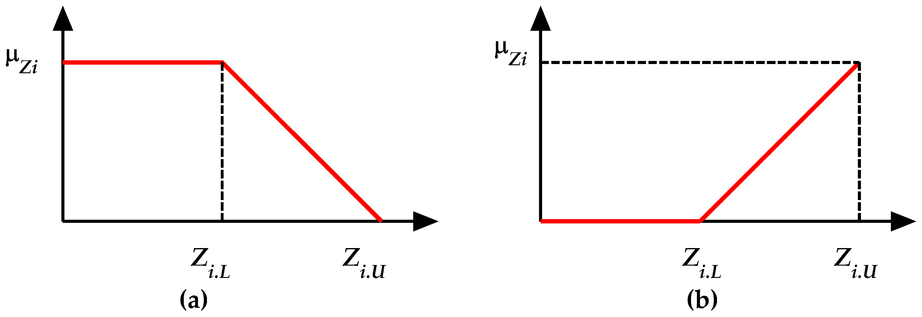
In the case of maximum, the objective function
is presented with a linear membership function as follows:
Figure 2 represents the linear membership function for objectives.
The linear membership function for restrictive conditions in type
is as follows:
where:
are the upper and lower limits for the relevant restrictive conditions.
are the values of
matrix, given by average values of criterion.
The linear membership function for restrictive conditions in type
is as follows:
The solution of the fuzzy linear optimization is performed by introducing a new variable
which serve for reorganization of the fuzzy problem by using the membership function. Introducing a new variable
, the problem is always from maximum.
The optimization models are always of the maximum of lambda.
The fuzzy linear models are formed for each objective. For qualitative and/or quantitative criteria with constant values the restrictive condition are such as these in the linear optimization model.
3.3. Stage 3 Ranking the Alternatives
The results of fuzzy linear models are recorded in fuzzy efficient results matrix [
].
where:
is the score of alternatives
for objective
.
The classical SIMUS method is applied in the case of certainty, i.e., when the criteria are set by one value.
The ranking procedure includes the following parts. First, the normalized fuzzy ERM matrix [ is compiled. Second, the criterion of ranking is determined.
The normalization of the fuzzy ERM matrix is made for example by the sum of all elements in each row.
where:
are the elements of the normalized ERM matrix [
.
The decision-maker could choose another method of normalization.
The procedure for ranking alternatives is as follows:
where:
is the participation factor of alternative
.
is determined as the number of participations of each alternative in each column of normalized ERM-fuzzy matrix [
is the sum of all elements in each column of [
The maximal values of criterion show the best alternative.
The weights of the objectives could be determined using normalized fuzzy ERM matrix [ The weights serve to evaluate the importance of criteria. The ERM matrix gives the relative weight of each objective using the process of fuzzy linear programming and fuzzy SIMUS method. For this purpose, the maximum value ( of each row in normalized fuzzy ERM matrix is determined. These values indicated the importance of each objective.
The weight of each objective
is determined as follows:
The initial decision-making matrices and the normalized ones are formed by using data presented in
Table 2. This study used the sum method to make the normalization.
Table 3,
Table 4 and
Table 5 show the normalized average matrix, the normalized lower matrix and the normalized upper matrix. The average matrix is formed based on Equation (2).
4. Results and Discussion
The new fuzzy SIMUS method was applied to evaluate alternatives for a transportation plan for intercity trains in railway passenger traffic. This study uses the criteria and alternatives defined in [
47]. The model was tested in the Bulgaria’s railway network.
The studied criteria to assess the transport plan are as follows:
C1—Frequency of services, pair trains/day.
C2—Frequency of train stops.
C3—Average distance travelled, km.
C4—Average operating speed, km/h.
C5—Reliability. A coefficient accounting for the average delay of trains is determined.
C6—Directness. If the alternative includes direct service: C6 = 1, otherwise: C6 = 0.
C7—Train capacity, seats/day.
C8—Direct operational costs, EUR/day.
The criterion directness (C6) is qualitative, while the other ones are quantitative. The values of criterion C6 are 0 or 1. For the criterion C5 only one value for each alternative is set.
The criteria frequency of services (C1), average distance travelled (C3), average operating speed (C4), directness (C6) and train capacity (C7) are of a maximum. The criteria frequency of train stops (C2), reliability (C5) and direct operational costs (C8) are of a minimum. The criterion reliability (C5) is solved taking into account of the train delays and is therefore of a minimum.
The model investigates nine alternatives of transport plan for intercity railway services, named A1–A9. The alternatives differ in the number of wagons in the composition and the category of trains. The categories of the trains are three: category 1—express trains with mandatory reservation and service of large centers (transport and administrative); category 2—intercity trains which serve additionally large centers and transport junctions, reservation required; category 3—fast trains which operates between intermediate stations, in this case the reservation is not needed. The model uses the number of wagons in the train-three or four, according the current situation in the Bulgaria’s railway network.
The studied alternative of transport plan of intercity trains in Bulgaria’s railway network are as follows:
A1—Three categories of trains—category 1, category 2 and category 3. The train composition consists 4 wagons.
A2—Three categories of trains—category 1, category 2 and category 3. The train composition consists 3 wagons.
A3—Three categories of trains—category 1, category 2 and category 3. Category 1 are composed with 3 wagons, the other two categories—with 4 wagons.
A4—Two categories of trains—category 1 and category 3. The other two categories are composed with 4 wagons.
A5—Two categories of trains—category 1 and category 3. The other two categories are composed with 3 wagons.
A6—Two categories of trains—category 1 and category 3. Category 1 are composed with 3 wagons, other—with 4 wagons.
A7—Two categories of trains—category 2 and category 3. Both are composed with 4 wagons.
A8—Two categories of trains—category 2 and category 3. The train composition consists 4 wagons.
A9—two categories of trains—category 2 and category 3. Category 2 are composed with 3 wagons, other—with 4 wagons.
4.1. Stage 1: Determination the Parameters of Multi-Criteria Model
The parameters of multi-criteria were formed in the first stage. The three initial values were determined on the basis of an analysis of the passengers transported on Bulgaria’s railway network for a ten-year period (2009–2019). An unevenness of about 4–5% was found (increase, decrease). This means a change in the number of trains, costs, and other indicators studied.
Table 2 shows the values of the criteria for all alternatives. For quantitative criteria, three values are set: lower, medium and upper. Criterion reliability (C5) is quantitative, but has the same values for upper, medium, and lower values. Both last columns of the table present the type of optimization and the operator for restrictive conditions in the SIMUS method.
4.2. Stage 2: Fuzzy SIMUS Procedure
The second stage of the methodology includes a definition of the fuzzy-SIMUS model. First, the SIMUS method is applied for normalized lower and normalized upper matrices in order to determine the values of objective functions.
For example, the SIMUS linear optimization model for a normalized lower matrix (
Table 4) for objective Z1 is presented as follows:
The objective function is:
Table 6 presents the restrictive conditions.
Table 7 represents the results for objective functions for upper and lower values of criteria (
and the threshold values of the criteria (
. These results are used in fuzzy linear models for membership functions. For objectives Z5 and Z6, the results are obtained by using the average matrix and SIMUS linear procedure.
The parameters of fuzzy SIMUS are prepared by using data in
Table 2.
Table 8 and
Table 9 represent the values of coefficients of membership functions for optimization functions and for restrictive conditions. The Equations (8)–(12) were applied.
The fuzzy linear models are formed for each objective. The restrictive condition for qualitative and/or quantitative criteria with constant values are such as these in linear optimization model.
For example, the fuzzy linear model for objective Z1 with membership function is as follows:
The objective function is:
where:
is a new variable.
The restrictive conditions for objective function Z
1 is:
The values of the coefficients of the unknown in Equation (28) are obtained by the first row of
Table 8. The value of the constant term in the Equation (27) are obtained by the sixth column in
Table 9.
Table 10 represents the restrictive conditions for the fuzzy linear optimization. For Z5 and Z6, the linear restrictive condition according to SIMUS method are defined. The procedure is applied for all fuzzy objectives. The results for the score of alternatives
for objective
is added in fuzzy efficient results matrix (FERM).
4.3. Stage 3: Ranking the Alternatives
The third stage of fuzzy-SIMUS method includes the ranking of alternatives. The Efficient results fuzzy matrix is formed.
Table 11 represents the results of FERM and the values of objectives. Each row indicates the values of the scores of the alternatives according to the optimization models. For example, the results show that the alternative A3 has a score 0.701 and alternative A5 has a score 0.298 by the first criterion. For objectives Z1-Z4 and Z7-Z8 are shown the results by applying fuzzy linear optimization. For objectives Z5 and Z6 are presented the results obtained by classical SIMUS model, as they have constants values. The last two columns of
Table 11 represent the value of objective functions for each fuzzy linear model (
and values of objectives Z5 and Z6 for linear models. The values of
do not affect the ranking.
Table 12 shows the normalized fuzzy efficient matrix and the ranking. The first part of the table consists the normalized fuzzy efficient matrix, and the second part show the ranking. The maximum value of each row in normalized fuzzy ERM matrix is determined. These values indicate the importance of each objective. The most important objectives for ranking are the frequency of train stops (Z2) and the direct operational costs (Z9) which have the maximum score.
The results indicates that the Alternative 3 is the best choice for it has the largest score.
It is necessary to bear in mind that SIMUS produces a ERM matrix, filled with optimal data in each row, and in so doing maps the original criteria into objectives. From here uses two different very well-known heuristic procedures, the simple weighted sum, and the outranking. From the first it obtains a ranking and from the second another ranking. The first ranking is shown in
Table 12. Both rankings have a particularity: both are identical. Both different procedures start from a matrix where the performance values in each criterion are optimal. That is, SIMUS using two different procedures, starting from the same matrix, produces the same ranking.
The ranking by outranking procedure is based on the determination project dominance matrix (PDM). For this purpose, is used the data in
Table 11.
Table 13 shows the results. The number of the rows and the columns in
Table 13 are equal to the number of alternatives. The number of dominances is determined for each objective. For example, for objective Z1 according
Table 11, the alternative A3 dominates over all others (value 0.701 is maximum for A3). Then, a “1” is placed in cells (A3;A1), (A3;A2), (A3;A4), (A3;A5), (A3;A6), (A3;A7), (A3;A8), (A3;A9). For objective Z2, the alternative A5 has a clear dominance over all others. This means that a “1” is placed in cell (A5;A1), (A5;A2), (A5;A3), (A5;A4), (A5;A6), (A5;A7), (A5;A8), (A5;A9). This procedure is performed sequentially for each objective. The values in each cell are summed. The sum of the rows (
) and the columns (
) is determined. The differences between the sum of the rows and columns (
−
) for the same alternative is calculated. These values serve for ranking the alternatives. The alternative with maximal value is the best.
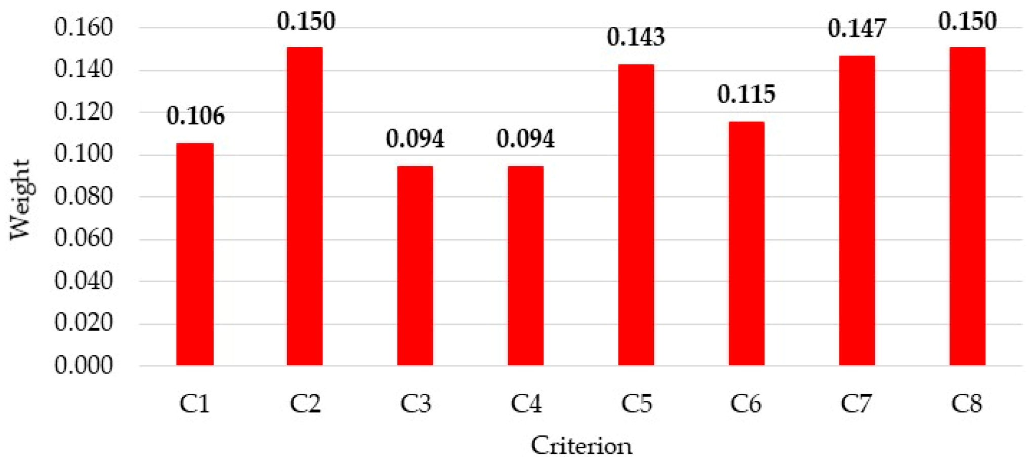
Figure 3 represents the weights of the criteria. The values are obtained by using Formula (24).
It can be concluded that the minimization of the frequency of train stops (C2), the minimization of the direct operational costs (C8) and the maximization of the train’s capacity (C8) have a great influence on the choice of a suitable alternative. The minimization of the train stops increases the operating speed, reduce the travel time and increase the directness of the trip. The maximization of the train’s capacity means to increase the composition of the train i.e., the number of wagons. These criteria are important for improving the quality of railway passenger transport and benefit both passengers and carriers. In this study, reliability (C5) was used to examine the accuracy of the train’s timetable. In this context, increasing the accuracy of the timetable also increases the confidence of passengers in the railway service. The directness means the train services a small number of intermediate stops for the route, i.e., reducing the travel time between the start and the end point. The maximization of the average distance travelled (C3) means attracting passengers for business and tourist travel, as well as increasing the level of preference for railway service. The maximation of the average operating speed means renewal of rolling stock for higher speeds, as well as reconstructions in railway infrastructure.
Increasing the average speed can also be realized by reducing the number of stops. The increase of the train’s frequency expands the convenience and the possibility of passengers to choose a trip.
4.4. Comparison with Classical SIMUS Approach
The fuzzy SIMUS approach can study the influence of the upper, medium, and lower values of criteria by comparing the rank of the alternatives with the classical SIMUS (without fuzzy).
Table 14 shows the results of ranking procedure for each of initial decision matrices with upper, average and lower values of criteria.
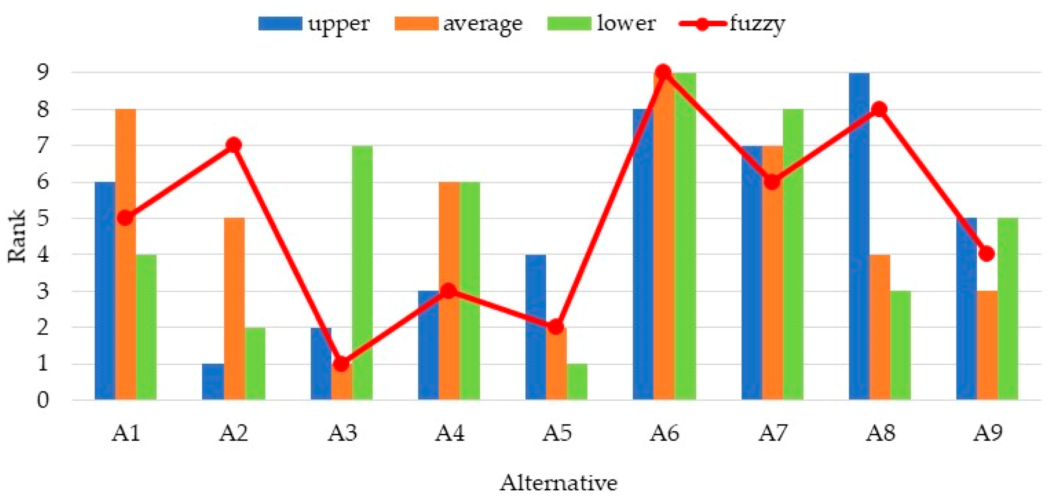
Figure 4 represents a comparison of the ranking by using upper, medium, and lower matrices and the classical SIMUS method, followed by the results obtained by applying the novel fuzzy SIMUS approach.
It can be concluded that there are differences in the ranking. Alternative A3 is the most suitable according to the medium matrix. Alternative A2 is the best according to the lower matrix. Alternative A5 is in the first position for the upper matrix. The fizzy SIMUS procedure puts in the first position the alternative A3. There are differences in the ranking for different positions by using both methods. It can be concluded that the change of the criteria, i.e., upper, middle, and lower values, change the choice of the most appropriate alternative, and these are respectively A2, A3, and A5.
The Fizzy SIMUS makes it possible to obtain the optimal solution in the case of uncertainty. Using fuzzy SIMUS, all elements of the system are considered and interacting. The method works with the optimal lower and upper values. At the same time, it obtains the relative importance of each criterion. The fuzzy SIMUS get two ERM matrices-upper and lower. In so doing, the scores for each alternative for upper and lower values are obtained, and then it would be possible to analyze how the rank is altered.
4.5. Verification of the Results
The authors compared the results obtained by fuzzy SIMUS with the results presented in paper [
47] because the problem solved is the same—three initial matrices (lower, medium, and upper) are set, and also the alternatives and criteria are the same. The methodology on [
47] is not used fuzzy approach but solved a problem in the case of uncertainty. The objective of both approaches is to determine the best alternative when the initial data are not precisely defined and are set with tree values.
To verify the results, the ranking was compared with these presented in [
47] where the same problem was solved by using SIMUS, AHP and Decision Tree methods in the case of uncertainty. The probability of a 10% reduction, saving, or 10% increase in passenger flow and it impact to obtain a sustainable transport plan solution were analysed. So, three matrices with lower, medium and lower values of criteria for each alternative were formed.
The values of the SIMUS ranking criterion for each of matrices and the AHP assessments of variation in passenger flows were used as input to the decision tree in the case of uncertainty. So, the suitable alternative was determined. It was found out that the best is the alternative A3.
To compare the level of coincidence between the results obtained by applying the fuzzy SIMUS method and the integration approach, including SIMUS, AHP, and decision tree methods [
47], the Spearman rank correlation coefficient
is used, [
50].
where
is the distance between the ranks for each data pairs, n is the number of elements.
This coefficient serves to determine the correlation between the ranking obtained by both approaches. The following scale is used: very weak—from 0.00 to 0.19; weak—from 0.20 to 0.39; moderate—from 0.40 to 0.59; strong—from 0.60—to 0.79; very strong—from 0.80 to 1, [
50]. The significant Spearman correlation coefficient value of 0.65 confirms that there is a strong correlation between both ranking.
Table 15 represents the results for Spearman correlation coefficient. The second column of the table shows the value of criterion of ranking by using the novel fuzzy SIMUS method, the third column presents the expected value for each alternative obtained in [
47], while the fourth and fifth columns show the rank obtained by both approaches.
It can be concluded that the results obtained by novel fuzzy SIMUS method are stable. Both approaches rank the same alternatives in first and second position. There are differences in the ranking of the other positions. This is due to the application of the AHP method where the expert assessments of the criteria were made.
The ranking of expected values for alternatives (
) shows that the first three positions are for alternative A3-A5-A2. The first two positions of the ranking using the SIMUS method for lower values of initial decision matrix are, respectively, the alternatives A5 and A2, and for upper values of the initial decision matrix the alternatives are A2 and A3. It is interesting to notice the near coincidences in [
47], the most important is the alternative 3, which is the second most important in upper values by using SIMUS procedure. The second is the alternative A5 which is the most important in low values. The third is the alternative A2 which is the most important in upper, and the second most important in [
47]. This indicates similarity in the results obtained.
4.6. Discussion
In this research, the new approach based on the fuzzy linear optimization and multi-criteria decision making is elaborated to determine the suitable alternative of transport plan of intercity trains on the railway network. The fuzzy logic is adapted to a MCDM method where there are no weights. Usually, in fuzzy, it works with a lower and an upper value adopting a certain function. These values are usually subjective. The difference using SIMUS is that those extreme values are optimal, since they correspond for each criterion to two optimal values, using linear programming, and are Pareto efficient.
Another advantage is that it allows to determine the degree of efficiency reached for each objective.
The optimal solution proposes service with three categories of intercity passenger trains. At present, the Bulgarian railway network serves 36 pairs of intercity trains and two categories of trains. The optimal scheme obtained from the fuzzy SIMUS model offers service between 38 and 42 pair trains per day which allows to increase the satisfaction of passengers’ needs. Three categories of intercity trains are proposed. The new category offers direct services with reduced number of stops for major routes in Bulgarian railway network.
On the other hands the operational costs for the proposed transport plan decrease. According to the existing transport plan they are 57701 EUR/day, while according to the offered service they are between 50515 EUR/day and 56472 EUR/day. This is due to the fact that according to the proposed model the transport scheme is kept within the limits of criteria changes. The number of passenger trains depends on the volume of passenger flows. The proposed model allows to determine the suitable alternative taking into account the variability of passengers as well as the impossibility in some cases to be precisely defined. The fuzzy approach and the linear programming allow the inclusion of the uncertainty factor in the construction of a mathematical model and to increase the adequacy of the results. The obtained results allow transport managers to make operational decisions to change the number of trains, without affecting the chosen optimal transport plan, i.e., routes, train categories, and train compositions. The proposed alternative is based on a set of factors that jointly influence decision making, taking into account the limits of their change.
5. Conclusions
In this paper is elaborated a novel fuzzy multi-criteria method for decision-making in the case of uncertainty. The major contributions of proposed methodology are as follows. (i) The new fizzy SIMUS multi-criteria method was developed. (ii) The criteria are considered as objectives and the assessment of alternatives is based on fuzzy linear optimization of each objectives. (iii) The multi-criteria and multi-objective approaches to decision making are combined to increase the adequacy of the results. (iv) The methodology also allows to solve problems when one part of the criteria is in a state of uncertainty and another is in a state of certainty. (v) The method does not use the weights of criteria. They can be determined in the end of optimization to determine its impact on the studied system. (vi) The decision-making process does not depend on subjective assessments. (vii) The novel method was applied to evaluate railway passenger transport planning.
The methodology was experimented with for planning railway intercity passenger transport in Bulgarian’s railway network. Nine alternatives and eight criteria were studied. It was found that the objective which influences ranking the most are the frequency of train stops (15%), direct operational costs (15%), and the train’s capacity (14.7%) and reliability (14.3%). The practical contribution of this research consists of the proposed transport plan of intercity passenger trains which includes three categories of trains (presented by Alternative 3). By applying this new approach, it is possible to improve the quality of railway passenger transport and thereby benefit both passengers and carriers.


