Least Squares Support Vector Machine-Based Multivariate Generalized Predictive Control for Parabolic Distributed Parameter Systems with Control Constraints

Abstract

This manuscript addresses a new multivariate generalized predictive control strategy using the least squares support vector machine for parabolic distributed parameter systems. First, a set of proper orthogonal decomposition-based spatial basis functions constructed from a carefully selected set of data is used in a Galerkin projection for the building of an approximate low-dimensional lumped parameter systems. Then, the temporal autoregressive exogenous model obtained by the least squares support vector machine is applied in the design of a multivariate generalized predictive control strategy. Finally, the effectiveness of the proposed multivariate generalized predictive control strategy is verified through a numerical simulation study on a typical diffusion-reaction process in radical symmetry.

1. Introduction

Modeling and control issues in the process industry involving distributed parameter systems (DPSs), which are infinite-dimensional systems, are challenging. The identification of unknown parameters of DPSs is much more complex than that of the lumped parameter systems (LPSs). In general, an infinite-dimensional problem is required to be approximated by finite-dimensional LPSs. Then, the model reduction methods are used to reduce the dimension of the approximate LPSs. For further details, see [1].

A system governed by parabolic partial differential equations (PDEs) is a typical DPS. It can be approximated by a set of low-dimensional ordinary differential equations through the use of Proper Orthogonal Decomposition (POD) technique [2], which is also called Karhunen-Loève expansion (K-L expansion) [3] or Principal Component Analysis (PCA) [4]. The POD technique is a popular technique for carrying out the task of model order reduction of parabolic systems. The spatial basis functions constructed from those slow modes of the system can capture the dominant dynamics while those fast modes can be ignored [5]. For the identification of the unknown parameters of the approximate LPSs constructed from the low-dimensional time-series, conventional approaches, such as projection transformation, can be used. The Singular Value Decomposition and K-L expansion is applied to construct a low-dimensional LPS with a simple structure. However, the accuracy of the approximation is low for a nonlinear DPS [6,7]. The K-L expansion combined with the neural network method can be applied to construct a sufficiently accurate approximation for a nonlinear DPS [8,9,10,11,12,13,14]. The support vector machine (SVM) is a general identification approach, and the least-squares support vector machine (LS-SVM) is its modified version. The LS-SVM, which simplifies the calculation by replacing inequality constraints with equality constraints, inherits the characteristics of the global optimization property and high generalization capabilities of SVM [15]. The model reduction approach based on the K-L expansion combined with LS-SVM is applied to regression problems that do not have a large amount of sample data. It is potentially applicable to a wide range of DPSs [16,17]. Several improved PCA methods are available in the literature, such as the incremental POD method [18], the adaptive POD method [19], the adaptive K-L/Fuzzy method [20], and the nonlinear-PCA method [21], for dealing with more complex nonlinear DPSs. For the nonlinear parabolic DPSs with time-dependent spatial domains, a temporally-local model order-reduction technique [22] and sparse POD-Galerkin methodology [23] are proposed and have been successfully applied to handle the moving boundary problem for a hydraulic fracturing process.

Generalized predictive control (GPC) strategy is introduced in [24,25]. Due to its simplicity for implementation, and excellent performance and robustness, it has been successfully implemented in a diversity of industrial applications from single-variable to multi-variable, and linear to nonlinear [26].

In this paper, we present a new multivariate GPC strategy used in conjunction with the POD technique to reduce the model order of weakly nonlinear DPSs of parabolic type. Then, the LS-SVM method is used to identify the unknown parameters of the low-dimensional time-series. Detailed methodology used to construct the generalized predictive temperature control in the tubular chemical reactor [27] will be discussed, and the control constraints and stability analysis will also be considered in the paper. The GPC based on SVM method has been successfully applied to LPSs with nonlinear characteristics [28,29,30]. The predictor obtained using the SVM method combined with the POD technique is found to have higher accuracy. It is applicable to a wider range of nonlinear DPSs. On the other hand, the GPC strategy used in conjunction with POD and recursive least square method has been applied to DPSs [31,32,33]. Thus, it is advantageous to combine GPC with SVM for the modeling and control of DPSs.

The remainder of this paper is structured as follows. First, the system equations are described in Section 2. Then, the POD and LS-SVM for regression are briefly introduced, and the POD and LS-SVM-based predictive model is derived in Section 3. The POD and LS-SVM-based multivariate GPC strategy is presented in Section 4. In Section 5, the numerical simulation of a diffusion-reaction process in radical symmetry is carried out to examine the effectiveness of the proposed algorithm in Section 3. The summary and future work of our paper are included in Section 6.

2. System Description

We consider a class of weakly nonlinear PDEs of parabolic type as given below:

$$\frac{\partial y(x,t)}{\partial t}=\mathcal{A}\frac{{\partial }^{2}y(x,t)}{{\partial }^{2}x}+\mathcal{B}u\left(t\right)+f(x,t,y(x,t),\frac{\partial y(x,t)}{\partial x}),$$

(1)

where t is the time variable, $x\in \Omega$ is the spatial variable, and $\Omega$ is the spatial domain, $y(x,t)$ is the controlled output variable, $u\left(t\right)$ is the control input variable, $\mathcal{A}$ and $\mathcal{B}$ are the linear operators in Hilbert space $\mathcal{H}$, and $f(·)$ is an unknown weakly nonlinear function. System (1) is applicable to model a variety of physical and biochemical processes, such as catalytic reaction rods, steel casting, and the snap oven [5].

For system (1), it contains an unknown weakly nonlinear function $f(·)$. To obtain accurate information of such a system, a sufficient number of sensors need to be placed along the spatial location. Due to actual physical conditions, only a small number of actuators is allowed to be mounted to observe the state. The input-output data are obtained from the actual production process under random signal excitation. The control algorithm is developed in three stages: In Section 3, the output ${\left\{y(x_m,t_n)\right\}}_{m=1,n=1}^{M,N}$ excited by the input ${\left\{u(k,t_n)\right\}}_{k=1,n=1}^{K,N}$ are used by the POD technique to reduce the dimensionality of the approximate model, and M, N, and K are, respectively, the number of the sensors, the sample duration, and the actuators. A low-dimensional time-series obtained after model order reduction is identified by LS-SVM. In Section 4, the POD used in conjunction with the LS-SVM-based multivariate GPC strategy is utilized to design the required controller through solving a receding horizon optimization problem at every sample period.

3. Model Reduction by POD and LS-SVM

The POD and LS-SVM-based model will be established in this section. Since a high dimensional output is not ideal for the design of the controller, the POD technique will be applied first to reduce the dimension of the model. Let the input $u(·,t)\in {\Re }^{K\times N}$, and let $y(x_m,t_n)\in {\Re }^{M\times N}$. The POD basis of rank ℓ can be calculated by Algorithm 1 proposed in [2].

Algorithm 1 Proper Orthogonal Decomposition (POD) basis of rank ℓ

Require: Snapshots ${\left\{y(·,t)\right\}}_{j=1}^M\subset {\Re }^M,PODrank\ell \le M$, where ℓ is the rank of the POD basis. Step 1. Set $Y={[y_1,\cdots ,y_M]}^T\in {\Re }^{M\times N}$. Step 2. Determine $R=Y{Y}^T\in {\Re }^{M\times M}$. Step 3. Compute eigenvalue decomposition $[\Psi ,\Lambda ]=eig\left(R\right)$. Step 4. Set ${\psi }_i={\Psi }_{·,i}\in {\Re }^M,and{\lambda }_i={\Lambda }_{ii},{\lambda }_1\ge {\lambda }_2\ge \cdots \ge {\lambda }_{\ell }\ge \cdots {\lambda }_M,fori=1,\cdots ,M$. Step 5. Compute $\mathcal{E}(\ell )={\sum }_{i=1}^{\ell }{\lambda }_i/{\sum }_{i=1}^M{\lambda }_M$. return POD basis ${\Psi }_{\ell }={\left\{{\psi }_i\right\}}_{i=1}^{\ell }$ and eigenvalues ${\left\{{\lambda }_i\right\}}_{i=1}^{\ell }$.

Choose the minimum ℓ such that $\mathcal{E}(\ell )\ge 99\%$. Then,

$$y_{\ell }(x,t)={\Psi }_{\ell }\left(x\right)Y\left(t\right)\in {\Re }^{M\times N},$$

(2)

$$Y\left(t\right)={\Psi }_{\ell }^T\left(x\right)y(x,t)\in {\Re }^{\ell \times N},$$

(3)

where ${\Psi }_{\ell }^{\left(i\right)}\left(x\right)$ and $Y^{\left(i\right)}\left(t\right)$, $i=1,\cdots ,\ell$, represent, respectively, the i-th basis function and the corresponding low-dimensional time-series, $Y\left(t\right)={[Y^{\left(1\right)}\left(t\right),\cdots ,Y^{(\ell )}\left(t\right)]}^T$. Due to the orthogonality of ${\Psi }_{\ell }^{\left(i\right)}\left(x\right)$, the $Y^{\left(i\right)}\left(t\right)$ are independent. Through the use of the LS-SVM approach proposed in [15], the i-th estimated value of the time-series is:

$${\widehat{Y}}^{\left(i\right)}\left(t_n\right)=w^{\left(i\right)T}{\varphi }^{\left(i\right)}\left(X^{\left(i\right)}\left(t_n\right)\right)+b^{\left(i\right)},$$

(4)

where $X^{\left(i\right)}\left(t_n\right)={[Y^{\left(i\right)}\left(t_{n-1}\right),\cdots ,Y^{\left(i\right)}\left(t_{n-ny}\right),u_1\left(t_{n-1}\right),\cdots ,u_1\left(t_{n-nu}\right),\cdots ,u_M\left(t_{n-1}\right),\cdots ,u_M\left(t_{n-nu}\right)]}^T$, $i=1,\cdots ,\ell$, $w^{\left(i\right)}$ is the scale factor, $b^{\left(i\right)}$ is the bias, ${\varphi }^{\left(i\right)}(·)$ is a function which maps the vector $X^{\left(i\right)}$ from function space into feature space. The optimization problem can be expressed as:

$$\left\{\begin{array}{c}\underset{w^{\left(i\right)},b^{\left(i\right)},{\xi }^{\left(i\right)}}{min}J(w^{\left(i\right)},{\xi }^{\left(i\right)})=\frac{1}{2}{w}^{\left(i\right)T}{w}^{\left(i\right)}+\frac{1}{2}{\gamma }^{\left(i\right)}\sum _{j=1}^N{\xi }^{\left(i\right)2},\hfill \\ s.t.Y^{\left(i\right)}\left(t_n\right)=w^{\left(i\right)T}\varphi \left(X^{\left(i\right)}\left(t_n\right)\right)+b^{\left(i\right)}+{\xi }^{\left(i\right)},j=1,2,\cdots ,N,\hfill \end{array}\right.$$

(5)

where ${\gamma }^{\left(i\right)}$ is the regularization factor, and ${\xi }^{\left(i\right)}$ is the relaxation factor. According to Lagrange multiplier method, the Lagrange function is:

$$\mathcal{L}(w^{\left(i\right)},b^{\left(i\right)},{\xi }^{\left(i\right)},{\alpha }^{\left(i\right)})=\frac{1}{2}{w}^{\left(i\right)T}{w}^{\left(i\right)}+\frac{1}{2}{\gamma }^{\left(i\right)}\sum _{j=1}^N{\xi }^{\left(i\right)2}-\sum _{j=1}^N{\alpha }^{\left(i\right)}\left(j\right)(w^{\left(i\right)T}\varphi \left(X^{\left(i\right)}\right)+b^{\left(i\right)}+{\xi }^{\left(i\right)}-Y_i),$$

(6)

where ${\alpha }^{\left(i\right)}$ is the Lagrange operator. Let $\partial \mathcal{L}/\partial w^{\left(i\right)}=\partial \mathcal{L}/\partial b^{\left(i\right)}=\partial \mathcal{L}/\partial e^{\left(i\right)}=\partial \mathcal{L}/\partial {\alpha }^{\left(i\right)}=0$, the coefficients ${\alpha }^{\left(i\right)}$ and $b^{\left(i\right)}$ are obtained through solving the following linear algebraic equations:

$$\left[\begin{array}{cccc}0& 1& \cdots & 1\\ 1& X^{\left(i\right)}{\left(t_1\right)}^T·X^{\left(i\right)}\left(t_1\right)+\frac{1}{{\gamma }^{\left(i\right)}}& \cdots & X^{\left(i\right)}{\left(t_1\right)}^T·X^{\left(i\right)}\left(t_N\right)\\ ⋮& ⋮& \ddots & ⋮\\ 1& X^{\left(i\right)}{\left(t_N\right)}^T·X^{\left(i\right)}\left(t_1\right)& \cdots & X^{\left(i\right)}{\left(t_N\right)}^T·X^{\left(i\right)}\left(t_N\right)+\frac{1}{{\gamma }^{\left(i\right)}}\end{array}\right]\left[\begin{array}{c}{b}^{\left(i\right)}\\ {\alpha }_1^{\left(i\right)}\\ ⋮\\ {\alpha }_N^{(i})\end{array}\right]=\left[\begin{array}{c}0\\ Y^{\left(i\right)}\left(t_1\right)\\ ⋮\\ Y^{\left(i\right)}\left(t_N\right)\end{array}\right],$$

(7)

The time-series $Y^{\left(i\right)}$ can be obtained as:

$$\begin{array}{cc}\hfill {\widehat{Y}}^{\left(i\right)}\left(t_n\right)=& \sum _{\tau =1}^N{\alpha }_{\tau }^{\left(i\right)}·{\mathcal{K}}^{\left(i\right)}\left(X^{\left(i\right)}\left(t_n\right),X^{\left(i\right)}\left(\tau \right)\right)+b^{\left(i\right)}\hfill \\ \hfill =& \sum _{j=1}^{ny}\sum _{\tau =1}^N{\alpha }_{\tau }^{\left(i\right)}{X}^{\left(i\right)}\left(\tau \right)\left[j\right]z^{-j}·Y^{\left(i\right)}\left(t_n\right)\hfill \\ & +\sum _{k=1}^K\sum _{j=1}^{nu}\sum _{\tau =1}^N{\alpha }_{\tau }^{\left(i\right)}{X}^{\left(i\right)}\left(\tau \right)[ny+(k-1)·nu+j]z^{-j}·u_k\left(t_n\right)+b^{\left(i\right)},\hfill \end{array}$$

(8)

where ${\mathcal{K}}^{\left(i\right)}(·,·)$ is the kernel function. The linear kernel function ${\mathcal{K}}^{\left(i\right)}\left(X^{\left(i\right)}\left(t_n\right),X^{\left(i\right)}\left(\tau \right)\right)=$$X^{\left(i\right)}{\left(t_n\right)}^T·X^{\left(i\right)}\left(\tau \right)$ is chosen, and $X^{\left(i\right)}\left(t_n\right)\left[j\right]$ is the j-th term of $X^{\left(i\right)}\left(t_n\right)$, $z^{-j}$ is the j-step backward shift operator.

The matrix form of the time-series autoregressive exogenous (ARX) model obtained by the LS-SVM approach is:

$$A\left(z^{-1}\right)Y\left(t\right)=B\left(z^{-1}\right)U(t-1)+b,$$

(9)

where $A\left(z^{-1}\right)=\mathit{I}-A_{\ell }$, $A_{\ell }=diag(A^{\left(1\right)},\cdots ,A^{(\ell )})$, $A^{\left(i\right)}={\sum }_{j=1}^{ny}{\sum }_{\tau =1}^N{\alpha }_{\tau }^{\left(i\right)}{X}^{\left(i\right)}\left(\tau \right)\left[j\right]z^{-j}$, $B\left(z^{-1}\right)={[B^{\left(1\right)},\cdots ,B^{(\ell )}]}^{\prime }$, $B^{\left(i\right)}=[B_1^{\left(i\right)},\cdots ,B_K^{\left(i\right)}]$, $B_k^{\left(i\right)}={\sum }_{k=1}^K{\sum }_{j=1}^{nu}{\sum }_{\tau =1}^N{\alpha }_{\tau }^{\left(i\right)}{X}^{\left(i\right)}\left(\tau \right)[ny+(k-1)·nu+j]z^{-j}$, $i=1,\cdots ,\ell$, and $b={[b^{\left(1\right)},\cdots ,b^{(\ell )}]}^T$, $k=1,\cdots ,K$.

4. POD and LS-SVM-Based Multivariate GPC

GPC strategy proposed in [23,24] is a class of predictive control algorithm developed for adaptive control due to its excellent performance and simplicity for implementation. It has been applied in a diversity of actual industrial plants during the past three decades. A multivariate GPC strategy will be proposed for parabolic DPSs with unknown coefficients in this section.

4.1. Multivariate GPC Strategy

Consider the following ARX model containing a zero-mean white noise:

$$A\left(z^{-1}\right)Y\left(t\right)=B\left(z^{-1}\right)U\left(t\right)+C\left(z^{-1}\right)\frac{e\left(t\right)}{\Delta },$$

(10)

where the output $Y\left(t\right)\in \ell \times 1$, the input $U\left(t\right)\in K\times 1$, and the white noise with zero mean $e\left(t\right)\in \ell \times 1$. $\Delta =1-z^{-1}$, $C\left(z^{-1}\right)$ is the identity matrix. Minimizing the quadratic cost function on a finite horizon to obtain the optimal control increment as follows:

$$J(N_p,N_u)=\sum _{j=1}^{N_p}\parallel \widehat{Y}(t+j|t)-w(t+j){\parallel }^2+\sum _{j=1}^{N_u}{\parallel \Delta u(t+j-1)\parallel }_{\lambda }^2,$$

(11)

where $\widehat{Y}(t+j|t)$ is the output predictive j-step ahead value based on previous state up to time t. $\lambda$ is the weighted coefficient of $\Delta u$. $N_p$ and $N_u$ are, respectively, the prediction horizons and control horizons. The reference trajectory $w(t+j)$ is defined as:

$$w(t+j)={\alpha }_{w}w(t+j-1)+(1-{\alpha }_w)Y_{sp}(t+j),$$

(12)

$$Y_{sp}(t+j)=\Psi {}^{\prime }\left(x\right)y_{sp}(x,t+j),$$

(13)

where $y_{sp}$ is the set point value. Consider the Diophantine equation:

$${\mathit{I}}_{\ell \times \ell }=E_j\left(z^{-1}\right)\tilde{A}+z^{-j}{F}_j\left(z^{-1}\right),$$

(14)

where $\tilde{A}=A\Delta$. The order of the polynomial matrix $E_j\left(z^{-1}\right)$ is $j-1$, and that of the polynomial matrix $F_j\left(z^{-1}\right)$ is $ny$. Since b is constant, $\Delta b$ is zero.

Let $E_j\left(z^{-1}\right)B\left(z^{-1}\right)=G_j\left(z^{-1}\right)+z^{-j}{G}_{jp}\left(z^{-1}\right)$ and $f_j=G_{jp}\left(z^{-1}\right)\Delta u(t-1)+F_j\left(z^{-1}\right)Y\left(t\right)$, the j-step prediction is:

$$\widehat{Y}(t+j|t)=G_j\left(z^{-1}\right)\Delta u(t+j-1)+f_j,$$

(15)

By solving $E_j\left(z^{-1}\right)$ recursively, the $N_p$-step prediction value $\widehat{Y}$ can be written as:

$$\left[\begin{array}{c}\widehat{Y}(t+1|t)\\ \widehat{Y}(t+2|t)\\ ⋮\\ \widehat{Y}(t+N_u|t)\\ ⋮\\ \widehat{Y}(t+N_p|t)\end{array}\right]=\left[\begin{array}{cccc}{G}_0& 0& \cdots & 0\\ G_1& G_0& \cdots & 0\\ ⋮& ⋮& \ddots & ⋮\\ G_{N_u}& 0& \cdots & G_0\\ ⋮& ⋮& \cdots & ⋮\\ G_{N_p-1}& G_{N_p-2}& \cdots & G_{N_p-N_u}\end{array}\right]\left[\begin{array}{c}\Delta u\left(t\right)\\ \Delta u(t+1)\\ ⋮\\ \Delta u(t+N_u-1)\end{array}\right]+\left[\begin{array}{c}{f}_1\\ f_2\\ ⋮\\ f_{N_u}\\ ⋮\\ f_{N_p}\end{array}\right],$$

(16)

where $G_j\left(z^{-1}\right)={\sum }_{i=0}^{j-1}{G}_i{z}^{-i}$. The matrix form of the prediction value $\widehat{Y}$ is:

$$Y=G\Delta u+f.$$

(17)

Rewrite the quadratic criterion (11) as:

$$J={(G\Delta u+f-w)}^T(G\Delta u+f-w)+\Delta u^T\lambda \Delta u,$$

(18)

If there are no constraints, the optimum $\Delta u$ without constraint can be obtained as:

$$\Delta u=H{G}^T(w-f),$$

(19)

where $H={(G^{T}G+\lambda \mathit{I})}^{-1}$. It is difficult to avoid control constraints in practical systems. The constrained incremental control law directly truncated at the boundary is not optimal. Considering the control constraints $\Theta \Delta u\le \theta$, the quadratic criterion using a Lagrange multiplier is given as follows [31]:

$$J(N_p,N_u)=\sum _{j=1}^{N_p}{\parallel \widehat{Y}(t+j|t)-w(t+j)\parallel }^2+\sum _{j=1}^{N_u}\left({\parallel \Delta u(t+j-1)\parallel }_{\lambda }^2+{\parallel \Theta \Delta u-\theta \parallel }_{\epsilon }^2\right),$$

(20)

where $\epsilon$ is the weighting marix of control constraint which is positive definite. The optimum $\Delta \tilde{u}$ with constraint can be obtained as:

$$\Delta \tilde{u}=\Delta u-H{\Theta }^T{(\Theta H{\Theta }^T+{\epsilon }^{-1})}^{-1}(\Theta \Delta u-\theta ),$$

(21)

The quadratic criterion is solved repeatedly at the subsequent sampling times, only the first term of $\Delta \tilde{u}$ is applied to the actual system, so the control action is:

$$u(k,t_j)=u(k,t_{j-1})+\Delta \tilde{u}(k,t_j),$$

(22)

where k, $k=1,\cdots ,K$, is defined in Section 2. The constrained control action is handled by the truncated algorithm:

$$u(k,t_j)=\left\{\begin{array}{cc}\hfill u_{min},& u(k,t_j)\le u_{min}\hfill \\ \hfill u(k,t_j),& u_{min}\le u(k,t_j)\le u_{max}\hfill \\ \hfill u_{max},& u(k,t_j)\ge u_{max}\hfill \end{array}\right.,$$

(23)

where $u_{min}\le u(k,t_j)\le u_{max}$.

The proposed POD and LS-SVM-based multivariate GPC algorithm can be summarized in Algorithm 2.

Algorithm 2 The POD and least-squares support vector machine (LS-SVM)-based multivariate generalized predictive control (GPC).

Require: A set of output $y(x_m,t_n)$ is derived by appropriate excitation signals. Step 1. POD basis ${\left\{{\psi }_i\right\}}_{i=1}^{\ell }$ and eigenvalues ${\left\{{\lambda }_i\right\}}_{i=1}^{\ell }$ are obtained by Algorithm 1. Step 2. The predictor $\widehat{Y}$ and the ARX model are built by LS-SVM with a linear kernel. Step 3. Compute $\Delta u$ by Equation (16). If the constrained condition is not satisfied, replaced $\Delta u$ with $\Delta \tilde{u}$ using Equation (18). Step 4. Use the control law $u(k,t_j)$ to the actual system at instant $t_j$. Step 5. Let $j=:j+1$, Repeat Step 3 and Step 4 at instant $t_{j+1}$.

4.2. The Stability Analysis

We assumed that the following assumptions are satisfied throughout:

Assumption 1.

The reference trajectory $w(t+j)$ is bounded, and the prediction error of model (8) is bounded.

Assumption 2.

System (1) is open-loop stable, so that the influence of the control action exerted at the past time tends to zero with the increase of time.

Assumption 3.

The fast modes of the dynamic of system (1) are ignored, so that it suffices to consider the stability conditions of the nominal system (9).

Assumption 4.

The future disturbances are equal to that at time t. The mismatch and any uncertainty of model (15) can be estimated as:

$$\widehat{D}(t+1)={[\widehat{d}{(t+1)}^T\cdots \widehat{d}{(t+N_p)}^T]}^T,$$

(24)

$$\widehat{d}(t+1)=ϵ(Y(t+1)-\widehat{Y}(t+1)),$$

(25)

where $Y(t+1)={\Psi }_{\ell }^T\left(x\right)y(x,t+1)$, and $0\le ϵ\le 1$.

The real value of the nominal system (10) at time $t+1$ are

$$Y(t+1)=\widehat{Y}(t+1)+\widehat{d}(t+1)=G_0\Delta u\left(t\right)+f_1+ϵ(Y\left(t\right)-\widehat{Y}\left(t\right)).$$

(26)

Assume that only $Y(t+1)$ and $u\left(t\right)$ are included in the closed-loop system. Then, $\tilde{Y}(t+1)=[Y(t+1)\Delta u\left(t\right)]$. Let $\mathcal{D}=-H{G}^T$, $\Delta u\left(t\right)={\mathcal{D}}_{1}FY\left(t\right)+{\mathcal{D}}_1$ where ${\mathcal{D}}_1$ is the first ℓ columns of $\mathcal{D}$. Substitute $\Delta u\left(t\right)$ into Equation (26). Then,

$$\tilde{Y}(t+1)=\left[\begin{array}{cc}A+B{\mathcal{D}}_{1}F& 0\\ {\mathcal{D}}_{1}F& \mathit{I}\end{array}\right]\tilde{Y}\left(t\right)+\left[\begin{array}{c}{\mathcal{D}}_1\\ {\mathcal{D}}_1\end{array}\right]\omega +\left[\begin{array}{c}e\left(t\right)\\ 0\end{array}\right].$$

(27)

Lemma 1.

(Unconstrained case) [6] If the eigenvalue ${\lambda }_i$ of the matrix A satisfy $|{\lambda }_i|<1$, then the closed-looped system is asymptotically stable, where

$$\tilde{A}=\left[\begin{array}{cc}A+B{\mathcal{D}}_{1}F& 0\\ {\mathcal{D}}_{1}F& \mathit{I}\end{array}\right].$$

(28)

Proof. 

By Assumptions 1 and 2, the output $\tilde{Y}(t+1)=\tilde{A}\tilde{Y}\left(t\right)+f_1\left(\omega \right)+f_2\left(e\left(t\right)\right)$ is bounded. Thus, the closed-looped system is asymptotically stable if that max $|{\lambda }_i|<1$ and $\parallel f_1\left(\omega \right)\parallel +\parallel f_2\left(e\left(t\right)\right)\parallel \le \delta$, where $\delta$ is a sufficient small number. By Assumption 3, system (1) is stable if the nominal system (10) is stable. □

Let $\tilde{\mathcal{D}}=(\mathit{I}-H{\Theta }^T{(\Theta H{\Theta }^{-1}+{ϵ}^{-1})}^{-1}\Theta )H{G}^T$, $\Delta \widetilde{u\left(t\right)}=\widetilde{{\mathcal{D}}_1}FY\left(t\right)+\widetilde{{\mathcal{D}}_1}$ where $\widetilde{{\mathcal{D}}_1}$ is the first ℓ columns of $\tilde{\mathcal{D}}$.

Lemma 2.

(Constrained case) [6] If the eigenvalue ${\tilde{\lambda }}_i$ of the matrix $\tilde{A}$ satisfy $|{\tilde{\lambda }}_i|<1$, then the closed-looped system is asymptotically stable, where

$$\tilde{A}=\left[\begin{array}{cc}A+B\widetilde{{\mathcal{D}}_1}F& 0\\ \widetilde{{\mathcal{D}}_1}F& \mathit{I}\end{array}\right].$$

(29)

Proof. 

The proof is similar to that given for Lemma 1. □

5. Case Study

The proposed multivariate GPC strategy is applied in the simulation study of an exothermic catalytic reaction in a long thin rod in radical symmetry, which has the form $A\to B$ [34] of transport reaction as shown in Figure 1.

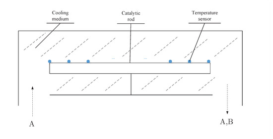
Figure 1. The schematic of the tubular reactor.

The goal is to produce as much product B as possible while consuming the least amount of energy by adjusting the axial cooling medium temperature. Assume that the density and the heat capacity of the rod are constant, and that the reaction rate of the rod is uniform. Due to radial symmetry, the dynamical distribution of the axial temperature on the rod is governed by the following PDE of parabolic type:

$$\frac{\partial T}{\partial t}=\frac{{\partial }^{2}T}{{\partial }^{2}x}+{\beta }_T\left(e^{-\frac{T}{1+T}}-e^{-\overline{\gamma }}\right)+{\beta }_u(T_c-T),$$

(30)

subject to the first kind of boundary conditions, and initial condition:

$$T(0,t)=0,T(L,t)=0,T(x,0)=T_0\left(x\right),$$

where t, x, and L are, respectively, the dimensionless time, axial position, and the length of reactor, and the controlled variables $T(x,t)$ and the control variables $T_c(x,t)$ are, respectively, the axial temperature and the cooling medium temperature of the reactor. In the simulation, let the length of the rod $L=\pi$, the initial temperature $T_0\left(x\right)=0.5$, the heat of reaction ${\beta }_T=50$, the heat transfer coefficient ${\beta }_u=2$, and the activation energy $\overline{\gamma }=4$. The 21 temperature sensors and 4 cooling medium temperatures $T_c(x,t)$ are equally located along the long rod. Each sample period $\Delta t=0.01$, and the total period is $t_s=2$. All the actual simulation values are calculated using Matlab PDE toolbox. The random excitation input signal that varies randomly between $-4$ to 1 are shown in Figure 2 and the corresponding output is shown in Figure 3.

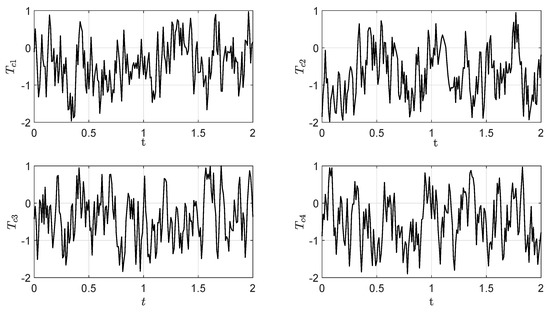
Figure 2. The random excitation input signal.

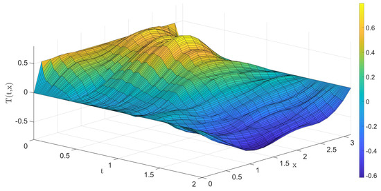
Figure 3. The corresponding output.

From Algorithm 1, the minimum number of the POD basis for ensuring $\mathcal{E}(\ell )\ge 99\%$ is 4. The first four basis functions $\varphi \left(x\right)$ are shown in Figure 4.

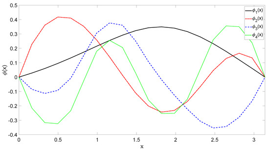
Figure 4. The first four Proper Orthogonal Decomposition (POD) basis functions.

The first 160 groups of data are used as training set, while the latter 40 groups of data are used as testing set. Then, the low-dimensional time-series ${\widehat{Y}}_T^{\left(i\right)}\left(t_n\right)$ are identified by LS-SVM:

$$\begin{array}{cc}\hfill {\widehat{Y}}_T^{\left(i\right)}\left(t_n\right)=& \sum _{j=1}^{ny}\sum _{\tau =1}^N{\alpha }_{\tau }^{\left(i\right)}{X}_T^{\left(i\right)}\left(\tau \right)\left[j\right]z^{-j}·Y_T^{\left(i\right)}\left(t_n\right)\hfill \\ & +\sum _{k=1}^K\sum _{j=1}^{nu}\sum _{\tau =1}^N{\alpha }_{\tau }^{\left(i\right)}{X}_T^{\left(i\right)}\left(\tau \right)[ny+(k-1)·nu+j]z^{-j}·u_k\left(t_n\right)+b^{\left(i\right)},\hfill \end{array}\left(31\right)$$

Different structures of the low-dimensional time-series model are considered for our numerical experiments, and the orders of $ny=4$ and $nu=3$ are finally selected for which the desired accuracy of the corresponding reduced dimensional model is achieved. The parameters $N=160$, and $K=4$. The 10-fold cross-validation is used to obtained the regularization factor $\gamma$. The LS-SVM-based model can approximate the low-dimensional time-series satisfactorily which is shown in Figure 5. The error of the predictive model is between $[-0.02,0.015]$ which is shown in Figure 6, and the mean of the root mean square error is $0.0001$. The average training times of the model are [16.4, 5.5, 20.5, 2.8] ms, respectively.

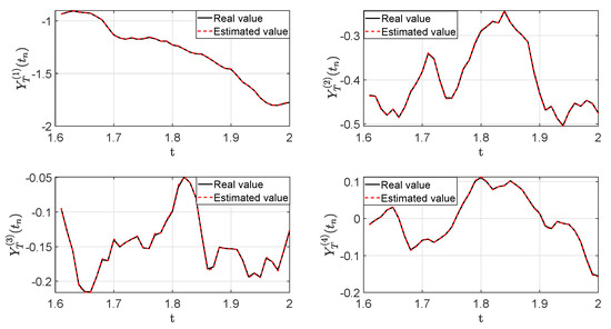
Figure 5. The performance of the least-squares support vector machine (LS-SVM)-based model.

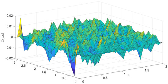
Figure 6. The prediction error of the POD used in conjunction with LS-SVM based model.

For expressions (11) and (12), choose $\lambda =1$, ${\alpha }_w=0.3$, $N_p=3$, $N_u=2$ as the parameters of the controller. The unconstrained control increment and control action are calculated by expressions (19) and (22), and the first column of the control variable $T_c$ is used in the actual system. The process is repeated at every sample period. The control variables $T_c$ and the output response curves for the unconstrained case are shown in Figure 7 and Figure 8, respectively.

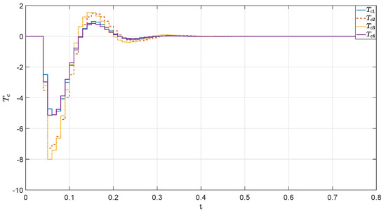
Figure 7. The control variables $T_c$ for the unconstrained case.

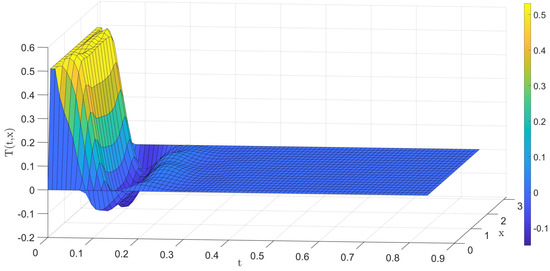
Figure 8. The output response curves for the unconstrained case.

In Figure 7 and Figure 8, the controller can quickly drive the system dynamics back to the steady-state in 30 sample periods, and the steady-state error is below $1\times {10}^{-5}$. From the simulation results, we can see that the proposed controller has excellent tracking performance and can be effectively applied to parabolic DPSs involving unknown coefficients. The fluctuation range of control variables between $-8$ to $1.5$ is large.

We now consider the case of control constraints. More specifically, $-0.5\le \Delta u\le 0.5$, and $-4\le u\le 1$. The constrained control increment and control action are updated by expressions (21) and (23). The control variables $T_c$ and the output response curves under the constrained case are shown in Figure 9 and Figure 10, respectively.

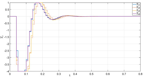
Figure 9. The control variables $T_c$ under the constrained case.

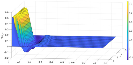
Figure 10. The output response curves under the constrained case.

In Figure 9 and Figure 10, we can see that the controller is working well in the case of control constraints. Due to the presence of the control constraints, the settling time is now extended to 50 sample periods. The time taken for control action calculation in each sampling period is given in Figure 11.

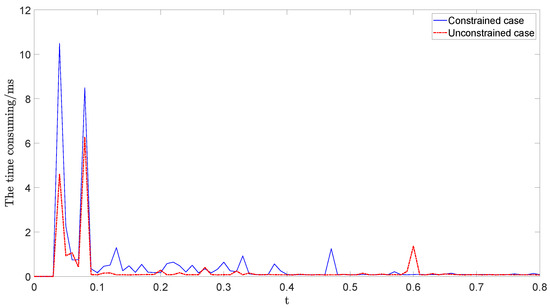
Figure 11. The time consuming of control law calculation.

In Figure 11, we can see that the time taken for unconstrained case is in milliseconds, and it is a bit longer for the constrained case.

6. Conclusions

A new control strategy, named POD and LS-SVM-based multivariate GPC, was developed for weakly nonlinear parabolic DPSs with unknown coefficients. The POD was used for model order reduction, resulting in low-dimensional lumped parameter systems. The desired control was designed based on this low-dimensional model. The LS-SVM with linear kernel function is found effective in the identification issues for linear and weakly nonlinear plants. An interesting question to ask is: Are there kernel functions for general nonlinear systems? The POD used in conjunction with the LS-SVM-based multivariate GPC strategy is easy to implement and is applicable to weakly nonlinear parabolic systems with unknown coefficients. As an illustration, a diffusion-reaction process was considered and solved using the proposed methods. The controller obtained has achieved the desired good performance. For future research, the online LS-SVM and radial basis kernel function will be applied to improve the modeling accuracy and to a more complex problem with nonlinearity. Furthermore, the method will also be extended to handle moving boundary problems, where the single POD basis function is replaced by a temporally-local basis function.

References

- Li, H.X.; Qi, C.K. Spatio-Temporal Modeling of Nonlinear Distributed Parameter Systems—A Time/Space Separation Based Approach; Springer: New York, NY, USA, 2007. [Google Scholar]
- Volkwein, S. Lecture: Proper Orthogonal Decomposition: Theory and Reduced-Order Modelling; Universtity of Konstanz: Konstanz, Germany, 2013. [Google Scholar]
- Mallat, S. A Wavelet Tour of Signal Processing-The Sparse Way, 3rd ed.; Elsevier: Singapore, 2009. [Google Scholar]
- Jolliffe, I. Principal Component Analysis, 2nd ed.; Springer: New York, NY, USA, 2002. [Google Scholar]
- Smyshlyaev, A.; Krstic, M. Adaptive Control of Parabolic PDEs; Princeton University Press: London, UK, 2010. [Google Scholar]
- Zheng, D.; Hoo, K.A. System identification and model-based control for distributed parameter systems. Comput. Chem. Eng. 2004, 28, 1361–1375. [Google Scholar] [CrossRef]
- Jing, X.T.; Li, H.X.; Lei, J.; Yang, N. KL-SVD based One-dimensional Modal Control combining with Diameter Control Subsystem as State Estimator in Czochralski Process. In Proceedings of the 9th International Conference on Intelligent Human-Machine Systems and Cybernetics, Hangzhou, China, 26–27 August 2017; pp. 189–192. [Google Scholar]
- Aggelogiannaki, E.; Sarimveis, H. Nonlinear model predictive control for distributed parameter systems using data driven artificial neural network models. Comput. Chem. Eng. 2008, 32, 1225–1237. [Google Scholar] [CrossRef]
- Li, H.X.; Deng, H.; Zhong, J. Model-based integration of control and supervision for one kind of curing process. IEEE Trans. Electron. Pack. Manuf. 2004, 27, 177–186. [Google Scholar] [CrossRef]
- Deng, H.; Li, H.X.; Chen, J.R. Delay-robust stabilization of a hyperbolic PDE-ODE system. IEEE Trans. Contr. Syst. Technol. 2005, 13, 686–700. [Google Scholar]
- Romijn, R.; Özkan, L.; Weiland, S.; Ludlage, J.; Marquardt, W. A grey-box modeling approach for the reduction of nonlinear systems. J. Process. Contr. 2008, 18, 906–914. [Google Scholar] [CrossRef]
- Bartecki, K. PCA-based approximation of a class of distributed parameter systems classical vs neural network approach. Bull. Pol. Acad. Sci. 2012, 60, 651–660. [Google Scholar] [CrossRef][Green Version]
- Wang, M.L.; Shi, H.B. Spatiotemporal prediction for nonlinear parabolic distributed parameter system using an artificial neural network trained by group search optimization. Neurocomputing 2013, 113, 234–240. [Google Scholar] [CrossRef]
- Wang, M.L.; Shi, H.B. An adaptive neural network prediction for nonlinear parabolic distributed parameter system based on block-wise moving window technique. Neurocomputing 2014, 133, 67–73. [Google Scholar] [CrossRef]
- Suykens, J.A.K.; Vandewalle, J. Least squares support vector machine classifiers. Neural Process. Lett. 1999, 6, 293–300. [Google Scholar] [CrossRef]
- Qi, C.K.; Li, H.X. A LSSVM Modeling Approach for Nolinear Distributed Parameter Processes. In Proceedings of the 7th World Congress on Intelligent Control and Automation, Chongqing, China, 25–27 June 2008; pp. 569–574. [Google Scholar]
- Qi, C.K.; Li, H.X.; Zhang, X.X.; Zhao, X.C.; Li, S.Y.; Gao, F. Time/Space-Separation-Based SVM Modeling for Nonlinear Distributed Parameter Processes. Ind. Eng. Chem. Res. 2011, 50, 332–341. [Google Scholar] [CrossRef]
- Xu, C.; Schuster, E. Model Order Reduction for High Dimensional Linear Systems based on Rank-1 Incremental Proper Orthogonal Decomposition. In Proceedings of the 2011 American Control Conference, San Francisco, CA, USA, 29 June–1 July 2011; pp. 2975–2981. [Google Scholar]
- Pourkargar, D.B.; Armaou, A. APOD Based Control of Linear Distributed Parameter Systems Under Sensor Controller Communication Bandwidth Limitations. AIChE J. 2013, 61, 434–447. [Google Scholar] [CrossRef]
- Lu, X.J.; Zou, W.; Huang, M.H. An adaptive modeling method for time-varying distributed parameter processes with curing process applications. Nonlinear Dynam. 2015, 82, 865–876. [Google Scholar] [CrossRef]
- Wang, M.L.; Qi, C.K.; Yan, H.C.; Shi, H.B. Hybrid neural network predictor for distributed parameter system based on nonlinear dimension reduction. Neurocomputing 2016, 171, 1591–1597. [Google Scholar] [CrossRef]
- Narasingam, A.; Siddhamshetty, P.; Kwon, J.S. Temporal clustering for order reduction of nonlinear parabolic PDE systems with time-dependent spatial domains: Application to a hydraulic fracturing process. AIChE J. 2017, 63, 3818–3831. [Google Scholar] [CrossRef]
- Sidhu, H.S.; Narasingam, A.; Siddhamshetty, P.; Kwon, J.S. Mohtadi and P. S. Tuffs, Model order reduction of nonlinear parabolic PDE systems with moving boundaries using sparse proper orthogonal decomposition: Application to hydraulic fracturing. Comput. Chem. Eng. 2018, 112, 92–100. [Google Scholar] [CrossRef]
- Clarke, D.W.; Mohtadi, C.; Tuffs, P.S. Generalized predictive control–Part I:the basic algorithm. Automatica 1987, 23, 137–148. [Google Scholar] [CrossRef]
- Clarke, D.W.; Mohtadi, C.; Tuffs, P.S. Generalized predictive control–Part II:extensions and interpetations. Automatica 1987, 23, 149–160. [Google Scholar] [CrossRef]
- Camacho, E.F.; Bordons, C. Model Predictive Control, 2nd ed.; Springer: New York, NY, USA, 2007. [Google Scholar]
- Ai, L.; Zhang, D.S.; Teo, K.L.; Deng, L.W. Generalized Predictive Temperature Control in Tubular Chemical Reactors by means of POD and LSSVM. In Proceedings of the 39th Chinese Control Conference, Shenyang, China, 27–29 July 2020; pp. 2407–2412. [Google Scholar]
- Iplikci, S. Support vector machines-based generalized predictive control. Int. J. Robust. Nonlin. 2006, 16, 843–862. [Google Scholar] [CrossRef]
- Iplikci, S. Online trained support vector machines-based generalized predictive control of non-linear systems. Int. J. Adapt. Control. 2006, 20, 599–621. [Google Scholar] [CrossRef]
- Guo, Z.K.; Guan, X.P. Nonlinear generalized predictive control based on online least squares support vector machines. Nonlinear Dynam. 2015, 79, 1163–1168. [Google Scholar] [CrossRef]
- Li, N.; Hua, C.; Wang, H.F.; Li, S.Y.; Ge, S.S. Time-Space Decomposition Based Generalized Predictive Control of a Transport-Reaction Process. Ind. Eng. Chem. Res. 2011, 50, 11628–11635. [Google Scholar] [CrossRef]
- Hua, C.; Li, N.; Li, S.Y. Time-space ARX modeling and predictive control for distributed parameter system. Control Theory Appl. 2011, 28, 1711–1716. [Google Scholar]
- Liu, P.F.; Tao, J.L.; Wang, X.G. Decoupling ARX Time-space model based GPC for distributed parameter system. In Proceedings of the 34th Chinese Control Conference, Hangzhou, China, 28–30 July 2015; pp. 612–617. [Google Scholar]
- Christofides, P.D. Nonlinear and Robust Control of PDE Systems: Methods and Applications to Transport-Reaction Processes; Birkhäuser: Boston, MA, USA, 2001. [Google Scholar]
Publisher’s Note: MDPI stays neutral with regard to jurisdictional claims in published maps and institutional affiliations. |
© 2021 by the authors. Licensee MDPI, Basel, Switzerland. This article is an open access article distributed under the terms and conditions of the Creative Commons Attribution (CC BY) license (http://creativecommons.org/licenses/by/4.0/).