Rotation Invariant Predictor-Corrector for Smoothed Particle Hydrodynamics Data Visualization

Abstract

In order to extract the vortex features more accurately, a new method of vortex feature extraction on the Smoothed Particle Hydrodynamics data is proposed in the current study by combining rotation invariance and predictor-corrector method. There is a limitation in the original rotation invariance, which can only extract the vortex features that perform equal-speed rotations. The limitation is slightly weakened to a situation that the rotation invariance can be used, given that a specific axis is existed in the fluid to replace the axis needed for it. Therefore, as long as the axis exists, the modified rotation invariant method can be used. Meanwhile, the vortex features are extracted by predictor-corrector method. By calculating the cross product of the parallel vector field, the seed candidates of vortex core lines can be obtained, and the real seed points can be gained from the rotation invariant Jacobian. Finally, the seed point and a series of candidates based on the predictor-corrector method are connected to draw the vortex core lines. Compared with the original method, the rotation invariant predictor-corrector method not only expands the application scope, but also ensures the accuracy of extraction. Our method adds the steps of calculating the rotation invariant Jacobian, the performance is slightly lower, but with the increase of the particle number, the performance gradually tends to the original method.

1. Introduction

There are different forms of vortex in nature, such as air and water. Generally, vortex is a spiral structure formed by rapidly rotating fluid. In hydrodynamics, Reynolds number Re can be used to study whether there is vortex separation near the object. When Re > 4000, the fluid is turbulent, and a large number of vortices will be produced.

Fluid flow analysis usually calculates a huge data set composed of various vectors and scalars. In order to solve the problem of tremendous calculation, it has become a new trend to extract flow features and screen valuable information through flow feature visualization. The extraction of vortex features has great research value and is widely used in medicine [1], ocean [2], aviation [3] and other fields. Therefore, how to extract vortex features accurately is a research hotspot in recent years.

Traditionally, flow visualization is classified into four categories: direct methods, geometry-based methods, texture-based methods and feature-based methods [4]. Vortex extraction belongs to the area of feature-based methods, and flow features can abstract data to reduce calculation. Recently, great progress has been made in the visualization of vortex features. However, there is still no formal definition of vortex, which leads to great divergence among researchers in the vortex extraction. Furthermore, the current vortex extraction methods still own many problems, such as over dependence on threshold, low accuracy and large amount of calculation.

Rotation invariance [5] proposed by Günther et al. is a reference frame invariant method, which can extract the vortices more accurately that perform equal-speed rotations. In this method, the rotation axis whose particles rotate around must be calculated in advance, so it cannot be used if frame performs any other type of movement. Besides, the predictor-corrector method [6] proposed by Schindler et al. calculates correcting points through multiple prediction and correction steps, so as to extract vortex core lines. This method has no rotation invariance, so it may fail when the reference frame rotates.

In the current study, a new rotation invariant method is put forward to calculate vortex core lines by predictor-corrector method. The research slightly reduces the constraint of rotation invariance so that it can be used under movement of the frame. By combining the rotation invariance and predictor-corrector method, rotation invariant vortex core lines are obtained, and then each vortex feature can be extracted more accurately.

The research applies rotation invariance under the general circumstance, and meanwhile weaken the effect of rotation factors on the accuracy of results. Firstly, a specific axis must be obtained as the rotation axis of modified rotation invariance. Secondly, points whose cross product of parallel vector field is 0 are defined as seed candidate of vortex features. When calculating the real seed points, the present study uses rotation invariant Jacobian instead of the general Jacobian. According to the predictor-corrector method, a series of candidates of each seed point are gained, and the vortex axis, namely, vortex core line, is extracted.

The main contributions of this research are as follows:

• Considering that original rotation invariance makes only sense for flows that induced by a rotating movement around an axis, there are some limitations. Hereby, the improvement of rotation invariance in the current study can be used in most cases.
• It employs the modified rotation invariant method rather than the predictor-corrector method, and meanwhile uses the modified Jacobian to calculate the seed points.
• When there are multiple rotating axes in data set, it divides the data set and extracts vortex core lines of each part respectively.

2. Related Work

2.1. Methods of Vortex Extraction

The frequently used methods of vortex feature extraction can be divided into four categories, including region-based, geometric and integration-based, machine learning-based and line-based methods, which are introduced briefly in this section. More importantly, as the line-based method is used in the present study to extract the vortex features, it may be primarily elaborated.

As we all know, the region-based method is used to extract vortices by calculating some physical quantity of particles, such as pressure [7] and helicity [8]. These methods have some disadvantages that the value of threshold has a direct impact on the results, such as lack of universality and error-causing in the extraction of weak vortex features. In recent years, Liu et al. introduced the Ω method, and found that when the threshold value Ω was 0.52, it had good adaptability to all situations, which reduced the influence of threshold on the results to a certain extent [9]. Nevertheless, the extraction results also had false-positive and false-negative, and the value of ε also had certain effect on the results.

For the geometric and integration-based method, it can be employed to extract vortex features by exploring the geometric features of streamlines or path lines, such as curvature rotation center method [10] and winding-angle method [11] proposed by Sadarjoen and Post. Because of the higher time complexity of this method and many limitations of its application in three-dimensional space, the use frequency is relatively low.

Recently, the machine learning-based method has attracted much attention. This method promotes the accuracy of vortex feature extraction by training the model in advance. Bin and Yi proposed a method based on a convolutional neural network (CNN). The results proved that the accuracy of result was as high as 96.67%. It can only extract the vortex features in the two-dimensional flow field. In addition, multiple artificial operations must be conducted [12]. Deng et al. proposed an objective extraction method, that is, in the preconditioning, IDV [13] method was used to mark the particles in the data set, and the CNN model was trained in the vortex network part. The output data of the preconditioning was sub-divided into vortex and non-vortex points [14]. The time complexity of this method is usually large, and a large number of data preconditioning must be calculated before the formal extraction of vortex features.

For the line-based method, it calculates the vortex axis (i.e., vortex core line) to extract vortex features. Sujudi and Haimes proposed an algorithm to extract vortices from three-dimensional vector fields. From their studies, one of the conditions for the existence of vortex core line was that Jacobian possessed complex eigenvalues [15]. Weinkauf et al. put forward the concept of feature flow field and extended Sujudi and Haimes method to unsteady flow. After adding time dimension, he deduced the formula of path line $P(x,y,z,t)$ under unsteady three-dimensional flow field, as follows,

$$P\left(x,y,z,t\right)=\left(\begin{array}{c}V\left(x,y,z,t\right)\\ 1\end{array}\right)=\left(\begin{array}{c}u\left(x,y,z,t\right)\\ v\left(w,y,z,t\right)\\ w\left(w,y,z,t\right)\\ 1\end{array}\right),$$

(1)

where V(x,y,z,t) is an unsteady 3D flow field. Moreover, Jacobian owns four eigenvalues e₁, e₂, e₃, 0 and their corresponding eigenvectors

$$\left(\begin{array}{c}{e}_1\\ 0\end{array}\right),\left(\begin{array}{c}{e}_2\\ 0\end{array}\right),\left(\begin{array}{c}{e}_3\\ 0\end{array}\right)=:e^S,f,$$

(2)

If two of these eigenvalues have imaginary components, vortex features exist, and the plane of the eigenvectors corresponding to the two eigenvalues are the plane of the vortex feature [16].

In most cases, the line-based method can be modified by calculating the parallel vector operator [17]. Peikert and Roth transformed Sujudi and Haimes method into finding the position where velocity v is parallel to the product of Jacobian matrix and velocity Jv, and replaced the complex steps of solving eigenvalues and eigenvectors through calculating matrix product [17]. Based on Fuchs et al., there were vortices in the region where $\nabla u·u\parallel u$, and the eigenvector n corresponding to the real eigenvalue was parallel to u [18]. Roth and Peikert proposed a method to extract vortices by solving the second derivative of velocity, and simplified Sujudi and Haimes method, that was, the vortices existed in a point, whose curvature is 0 or the velocity v and acceleration a are parallel [19].

However, there are still some problems in the line-based method, as following. A large number of Jacobian eigenvalues are calculated in this method. And the time complexity is high. Last but not least, in the steps of drawing, vortex core line is easy to be broken into multiple parts.

2.2. Reference Frame Invariance

Vortex extraction can also be classified according to the motion types of the reference frame. When extracting the vortex features, the motion of the reference frame does not affect the extraction of the vortex features, so various reference frame invariant methods are created, such as Galilean invariance, Lagrange invariance and rotation invariance.

Generally, many vortices are defined with Galilean invariant. Jeong and Hussain proposed λ₂-method, who extracted the vortex features by the second eigenvalue less than 0 [20]. And Sahner et al. adopted parallel vector to extract Galilean invariant ridge line or valley line [21]. When the reference frame is moving at a constant speed, the result of Galilean invariant vortex extraction is invariant. Nevertheless, there are certain errors in Galilean invariance when the reference frame is moving in other forms.

Ideally, Lagrange invariance, also famous for its objectivity, is the best method for vortex extraction. Objectivity means that, no matter what kind of motion the reference frame makes, the extraction results are objective and invariant. Tabor et al. shifted the Q-criterion [22] into an objective form, and extracted the vortex by solving the time derivative of the unit eigenvector of the strain rate tensor S [23]. Hadwiger et al. combined the global and local reference frame to calculate the time-dependent observer velocity field and approximate killing field, and accurately extracted the vortex features under different observing perspectives [24]. Additionally, Günther and Theisel extracted the Lagrangian invariant vortex features of inertial particles. But it is necessary to calculate six-dimensional parallel vector field, which greatly affected the performance [25]. At present, most of the objective methods still have strong restrictions on the vortex, so the expected extraction results are almost impossible to obtain. Moreover, the computation is more complex than the rotation invariant methods and Galilean invariant methods.

Rotation invariance [5] is a new concept proposed in recent years, which is used to extract vortices that perform equal-speed rotations more accurately. A vortex measure is rotation invariant if for any transformation, rotation invariant reference frame x’ is as follows:

$$x^{\prime }=Q\left(t\right)\left(x-x_0\right)+x_0,$$

(3)

where Q(t) is the constant velocity rotation matrix and x₀ is the rotation center. Compared with Galilean invariance, rotation invariance can extract the vortex features of rotating fluid more accurately.

Most of Galilean invariant methods can be transformed to rotation invariance, such as Q-criterion [22] and λ₂-criterion [20]. By changing the Jacobian J in the original method to the rotation invariant Jacobian Jr, we have

$$S_r=\frac{1}{2}\left(J_r+J_r^T\right),{\mathsf{\Omega }}_r=\frac{1}{2}\left(J_r-J_r^T\right),$$

(4)

Then, the rotation invariant strain rate tensor Sr and the rotation invariant vorticity tensor ${\mathsf{\Omega }}_r$ are obtained. Q-criterion and λ₂-criterion can be modified into the following rotation invariant form

$$\begin{array}{c}{Q}_r=\frac{1}{2}\left(\parallel {\mathsf{\Omega }}_r{\parallel }^2-\parallel S_r{\parallel }^2\right)>0\\ {\lambda }_{2r}={\lambda }_2\left(S_r^2+{\mathsf{\Omega }}_r^2\right)<0,\end{array}$$

(5)

When Sr and ${\mathsf{\Omega }}_r$ satisfy formula (5), the vortex features are extracted.

One limitation of this method is that the researcher must get the rotation center and the rotation axis in advance. A detailed description of rotation invariance is given in the Section 3.2.

3. Rotation Invariant Predictor-Corrector Method

The rotation invariant predictor-corrector method implements a direct algorithm:

• Calculate the cross product V × W at each particle;
• If V × W = 0:

  2.1.

  Extract the point as a seed candidate;

  2.1.

  Calculate rotation invariant Jacobian J_r;

• If there is a virtual eigenvalue in Jr, the point is extracted as a seed point;
• By multiple prediction and correction steps, the correcting points are calculated;
• Connect the seed point and correcting points to get a vortex core line.

The text continues here.

3.1. Extracting Seed Candidates by Parallel Vector Field

It is a tedious step to calculate Jacobian and its eigenvalues for each particle in the data set. Especially, when computing large data sets, it obviously becomes a key part that affects performance. Therefore, before extracting seed points, parallel vector field is used to preprocess the data set. In this step, it is required to screen quickly and simply. Herein, points satisfying the condition of parallel vector field are called seed candidates.

In this study, the seed candidates are extracted by searching for the parallel parts of two vector fields V and W in the fluid. Generally, at least one of the two vector fields V and W involves velocity gradient. And we use Levy criterion [8] to calculate cross products.

According to Levy criterion, we have

$$\begin{array}{c}{V}_i=u_i\\ W_i=g_{i+2}^{i+1}-g_{i+1}^{i+2}\\ \nabla V_i=\nabla u_i\\ \nabla W_i=\nabla g_{i+2}^{i+1}-\nabla g_{i+1}^{i+2},\end{array}$$

(6)

where u is the velocity and $g^i=$($g_i^1,g_i^2,g_i^3$) is a particle attribute, $\nabla V$ is the velocity gradient, then the seed candidates are extracted where V × W = 0. Due to practical reasons, the number of seed candidates whose cross products are exactly 0 may be too small. In this case, a threshold close to 0 is set, and points whose cross products are within the threshold range are regarded as seed candidates.

Meanwhile, the smoothed particle hydrodynamics (SPH) method is used to regard the fluid as a large number of particles which have the same size, each particle carries three-dimension positions, velocity, acceleration, mass and other attributes. Furthermore, A(r) of all particles in the neighborhood are weighted and summed to calculate a certain attribute A(r) of particles, e.g., gⁱ, and it satisfies

$$A\left(r\right)={\displaystyle \sum }_j{m}_j\frac{A_j}{{\rho }_j}W\left(r-r_j,h\right)$$

(7)

where m_j is particle mass, ρ_j is particle density, and W (r−r_j, h) is the SPH kernel. In order to reduce the time complexity, the data in the raw data set is directly used for cross product calculation. Through the comparative experiment, it is found that the error is too small to be noticed.

3.2. Extracting Seed Points by Modified Jacobian

It is a necessary condition for the existence of vortex that Jacobian has complex eigenvalues. Therefore, eigenvalues of Jacobian of seed candidates are calculated. Only candidates with complex eigenvalues can be taken as the real vortex seed points. And when calculating Jacobian, it is necessary to search the neighborhood of SPH particles. In order to reduce the time complexity, we use the consistent grid to segment three-dimensional space, in which the edge length of each grid is 1.5 times the particle radius, which is the same as neighborhood range set in experiment. When searching the neighborhood in three-dimensional space, only two kinds of points will be searched, including the points in the grid located by the seed candidate and the points that belong to its around 3 × 3 × 3 grid. Then, particles whose distance from the seed point is 1.5 times less than radius are searched in these grids.

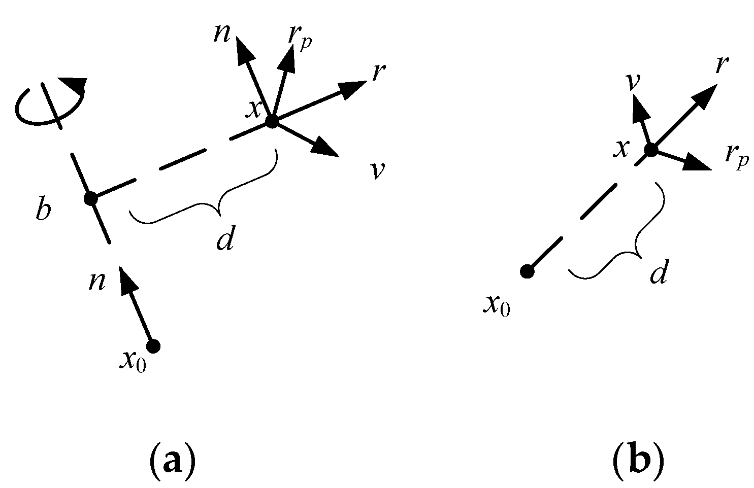
Next, the seed points are extracted under rotation invariant frame. Firstly, the rotation center and axis which the fluid around are calculated, as shown in Figure 1. Herein, x₀ is the rotation center, n is the three-dimensional rotation axis, and x is a particle in data set, whose rotation center is x₀. A vertical line is made through point x, which intersects the rotation axis n at point b, v is the velocity of particle.

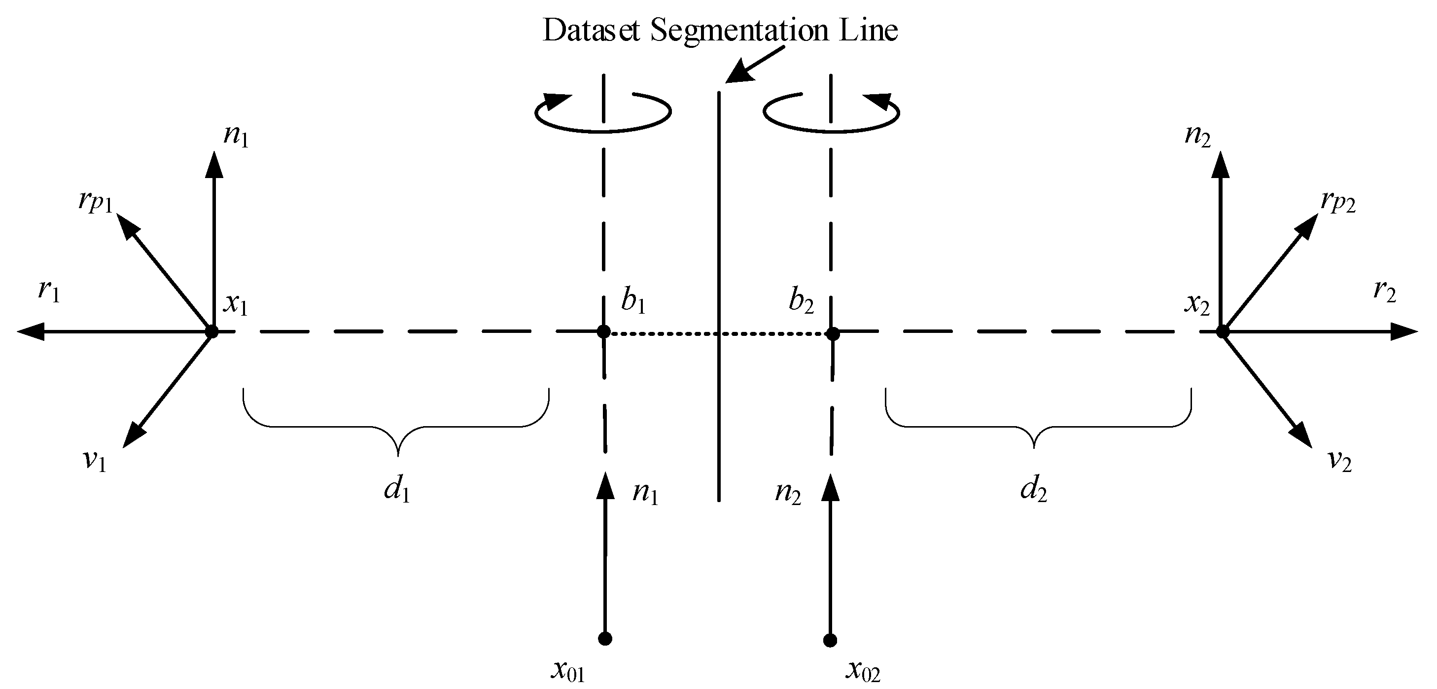
When data set has more than one rotation axis, it is segmented and the vortex features are extracted independently. Here we illustrate the case where there are two axes in the data set, as shown in Figure 2. x₀₁ and x₀₂ are two rotation centers, so the data set is divided into two parts. A line (a plane in 3D space) parallel to the z axis is made through the midpoint of segment b₁b₂. This line (plane) is used as the dataset segmentation line (plane).

After the step of dataset segmentation, the complex scene is divided into several simple scenes with a single rotation center, then the modified rotation invariance method is used.

The size and density of elements have changed after domain transformation, in this case, calculation of Jacobian is complicated, so the calculation of rotation invariant Jacobian $J_r$ is still carried out in Cartesian frame. We have

$$J_r=J+\frac{1}{d}RH{R}^T,$$

(8)

where $d=\parallel x-b\parallel ,R=\left(r_p,r,p\right),r=\frac{x-b}{d},r_p=r\times n$, and the three-dimensional matrix

$$H=\left(\begin{array}{c}-v^{T}r -v^T{r}_p 0\\ v^T{r}_p 0 0\\ 0 0 0\end{array}\right),$$

(9)

The rotation invariant Jacobian J_r and its eigenvalues are calculated by formulas (8) and (9). Only the seed candidates with complex eigenvalues of rotation invariant Jacobian will become the real seed points, the remaining seed candidates are discarded. In order to reduce the calculation time of Jacobian, the neighborhood of SPH particles is set to 1.5 times the particle radius, so that the neighborhood range is minimum and reliable.

3.3. Predictor-Corrector

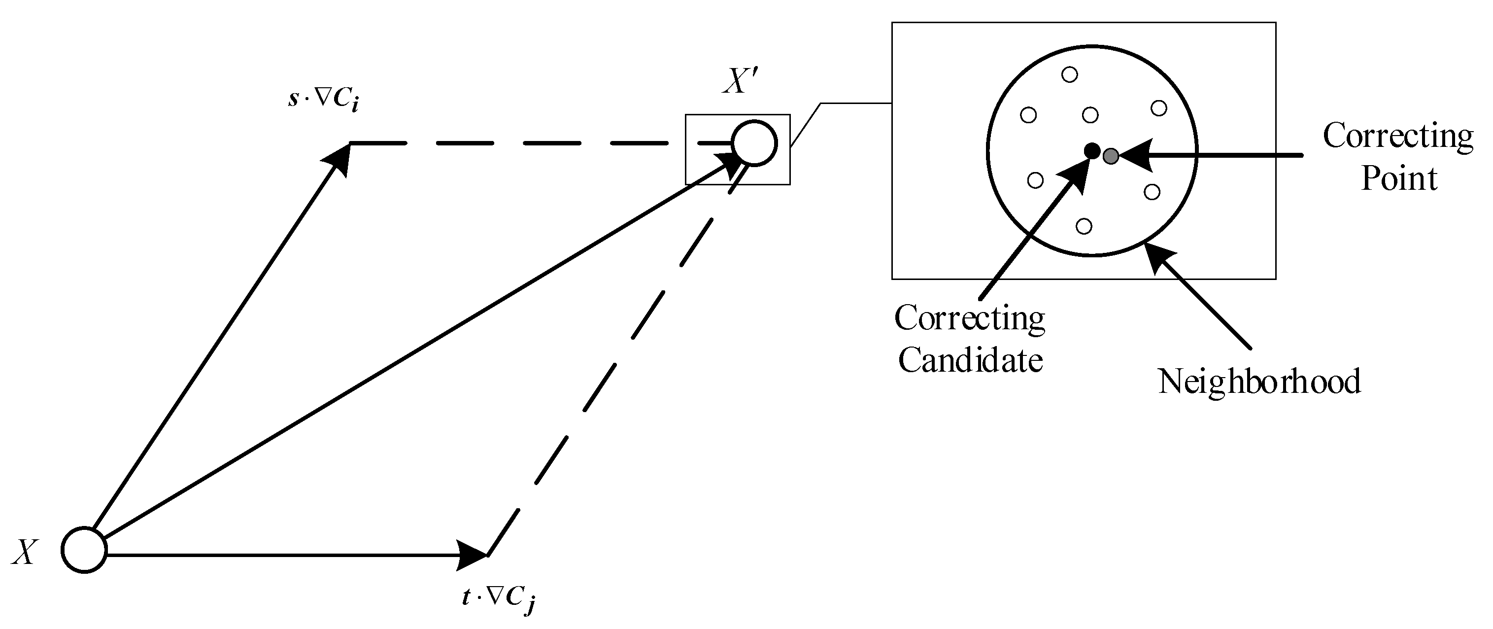
The vortex core line is connected by a series of correcting points starting from seed point. The step of finding the next correcting point from the seed point or one correcting point is called predictor-corrector. First, we calculate the gradient $\nabla C_1,\nabla C_2,\nabla C_3$ of the component of C = (C₁, C₂, C₃) = V × W and select the largest pair i, j of $\nabla C_i\times \nabla C_j$, if the value of cross product is positive, the cross product direction is taken as the tangent direction of vortex core line; if negative, the opposite direction is taken. The position of correcting candidate

$$X^{\prime }=X+s·\nabla C_i+t·\nabla C_j,$$

(10)

where X is the position of the seed point or previous correcting point, s and t are variable, which are used to calculate the step size of prediction. At the position of correcting candidate X’, we have

$$C_k{}^{\prime }\approx C_k+\left(s·\nabla C_i+t·\nabla C_j\right)·\nabla C_k=0,$$

(11)

where, k = i or j. The correcting candidate X’ is calculated by solving s and t and bringing them into formula (10). Here we consider a practical problem, if the correcting candidate does not belong to any particle in the data set, it will be regarded as the nearest particle in the neighborhood as the real correcting point, and also the starting point of the next prediction step, as shown in Figure 3. If there are no other points in the neighborhood, the prediction and correction step of seed point X is finished.

If the correcting points obtained by the prediction and correction steps still meet the vortex constraint, that is, the Jacobian has complex eigenvalues, the above prediction and correction steps are repeated. When the Jacobian has only real eigenvalues, or there is no other particle in the neighborhood of candidate, or reaches the boundary of fluid, the vortex core line of this seed point is finished.

In the drawing step, the correcting points which belong to the same seed point are connected by Bezier curve, and they compose the vortex core line. Coordinates B(T) of points on Bezier curve can be described as

$$\begin{array}{ll}\hfill B\left(T\right)={\displaystyle {\displaystyle \sum }_{i=0}^n}\left(\begin{array}{c}n\\ i\end{array}\right)& {\left(1-T\right)}^{n-i}{T}^i{P}_i\hfill \\ & =\left(\begin{array}{c}n\\ 0\end{array}\right){\left(1-T\right)}^n{T}^0{P}_0+\left(\begin{array}{c}n\\ 1\end{array}\right){\left(1-T\right)}^{n-1}{T}^1{P}_1+\dots \hfill \\ & +\left(\begin{array}{c}n\\ n-1\end{array}\right){\left(1-T\right)}^1{T}^{n-1}{P}_{n-1}+\left(\begin{array}{c}n\\ n\end{array}\right){\left(1-T\right)}^0{T}^n{P}_{n,}\hfill \end{array}$$

(12)

where T∈[0,1], T = i/(n + 1), and P₀, P₁, ..., P_n−1, P_n are the control points of Bezier curve, namely seed point and a series of correcting points.

In order to have a better extraction result, Bezier curve will show vortex strength and direction of vortex core line. Since the absolute value of imaginary part of Jacobian eigenvalue is positively correlated with the vortex strength, we take the absolute value as vortex strength and display it in the form of the width of Bezier curve. By changing the width between two control points, a vortex core line with a positive correlation between width and vortex strength is obtained. As shown in Figure 4, where X₀, ..., X₅ are the control points of Bezier curve. The RGB color gradient is used to represent the direction of vortex core line. From the seed point to the last correcting point, the RGB value changes from (255, 0, 0) to (0, 0, 255).

4. Results

Based on the rotation invariant predictor-corrector method, we implemented two sets of experiments of vortex feature extraction and compared with the original predictor-corrector method in the same experimental condition. The experiments are carried on a system with an AMD Ryzen 5 2600 CPU with 8 GB RAM, and the drawing step uses OpenGL library.

We mainly take four sets of experiments, and each step has a comparative experiment to confirm the accuracy of our method. Moreover, the comparative experiment uses the original predictor-corrector method [6]. In order to reduce the occlusion of sight, particle radius in the figures is reduced by 10 times.

The first test data set is SPH simulation for tracking cylinder movement, as shown in Figure 5, which is described as follows. There is a vertical cylinder in right half of the cuboid tank with fluid, and the lower part of the cylinder is in fluid. The data set simulates its movement to the left. In addition, there are 78,988 fluid particles and 8000 time steps in the test data set.

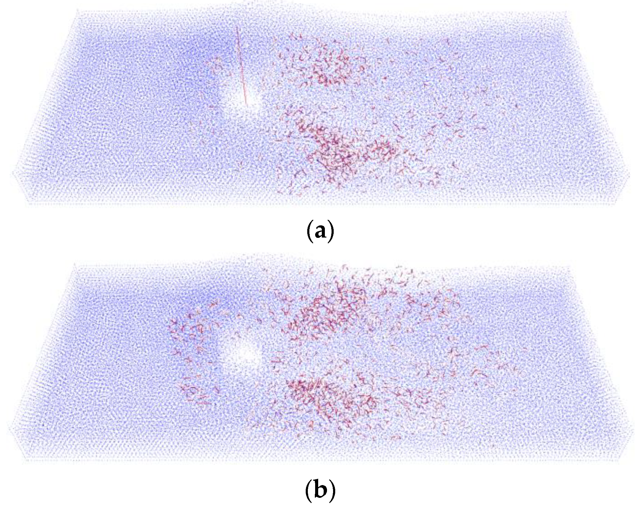
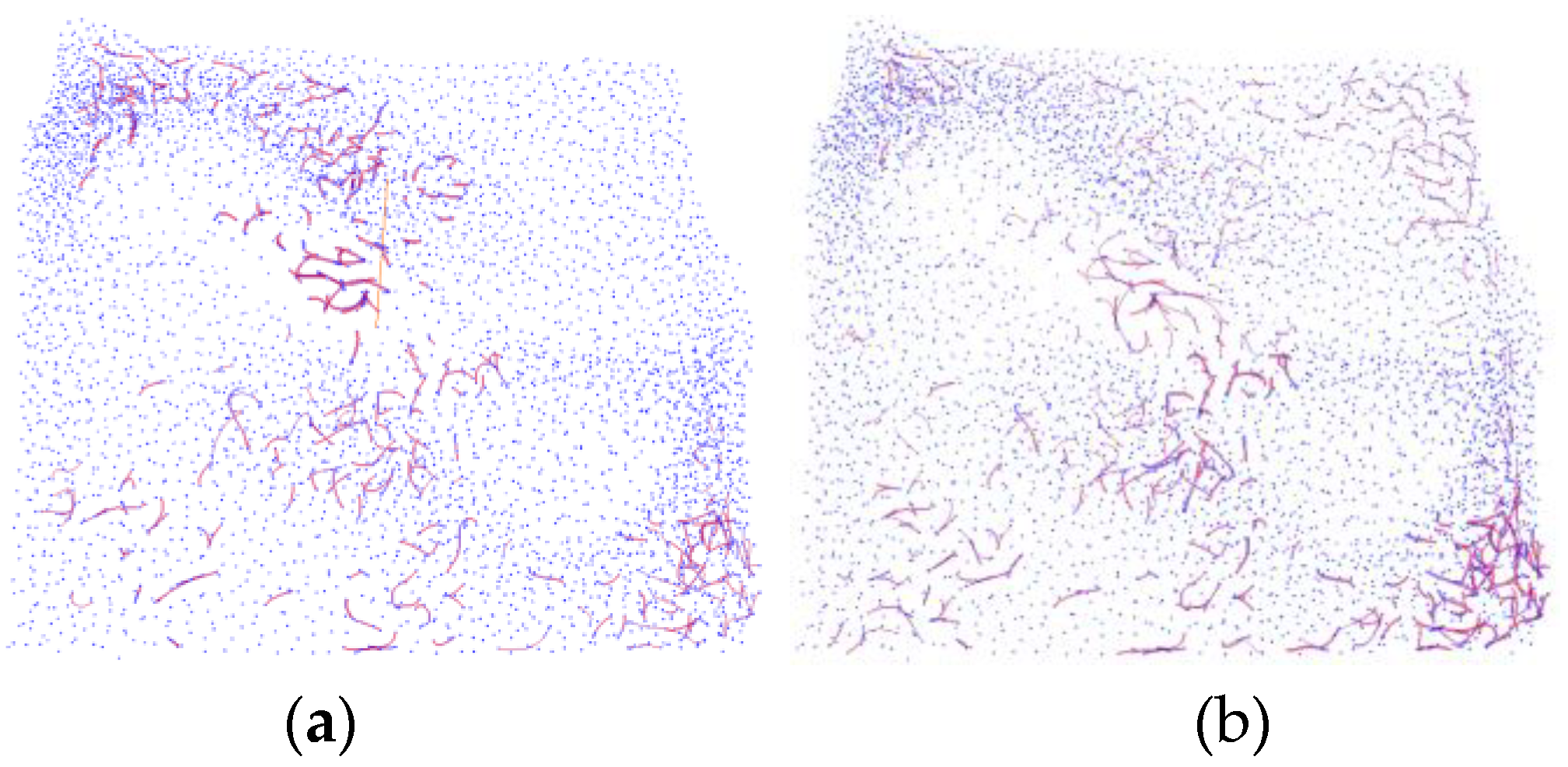
The vortex core line extraction results are shown in Figure 6 when cylinder moves to the 4968 time step. For instance, Figure 6a shows the rotation invariant vortex core line extraction, and Figure 6b displays the vortex core line extraction in the comparative experiment. At this time step, Re = 43, so the condition of generating Karman vortex street has not been reached. When fluid passes round the cylinder, it does not produce regular vortex features, and only generate features on both sides of the moving path of the cylinder. The beginning part of vortex core line is red, and it turns blue gradually. The width and density of vortex core line is positively correlated with the strength of vortex. The red line in Figure 6a is the rotation invariant axis. In the step of selecting rotation axis, we carry out many experiments and finally extract a particle which is always near the bottom rotation center of the cylinder. Starting from the particle, a straight line along the z-axis direction in three-dimensional space is made as the rotation invariant axis.

Because the velocity of fluid around the cylinder is faster than that of other regions, differences between the extraction results can be clearly seen. Furthermore, there is less false positive in our method. Compared with the original predictor-corrector method, it can reflect the vortex feature region more clearly and accurately.

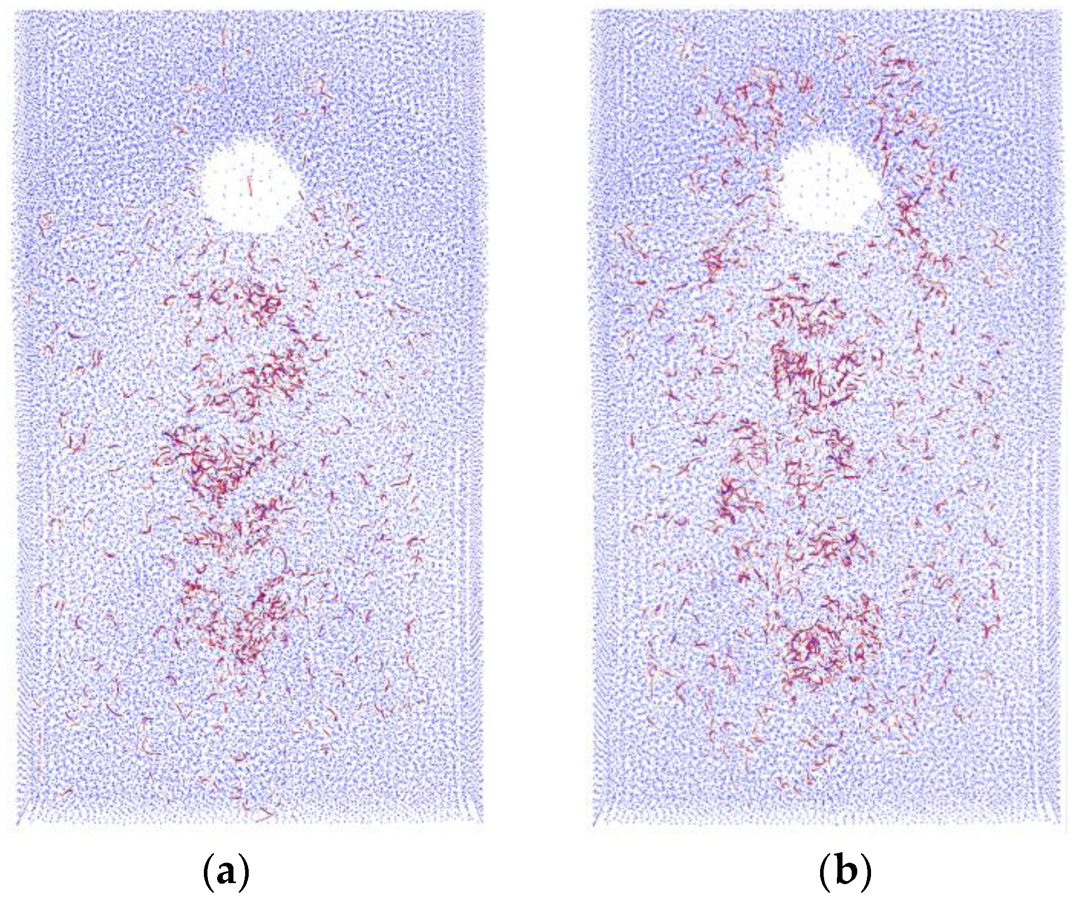
The second test data set is used to simulate the Karman vortex street. In this simulation, a cylinder obstacle is fixed and fluid particles move from top to bottom. There are 71,352 fluid particles and 500 time steps in the test data set. Besides, in Figure 7, the extraction results with Re = 70 has been shown. Moreover, Figure 7a presents the rotation invariant vortex core line extraction, and Figure 7b depicts the vortex core line extraction in the comparative experiment. The round blank part in figure is the position of cylinder. In Figure 7a, the red line at the center of obstacle is the rotation invariant axis.

Theoretically, Karman vortex street has been generated when Re = 70, and vortices with opposite rotation direction and regular arrangement are extracted behind the obstacle. However, the original predictor-corrector method owns many false positives around obstacle and feature regions. Compared with the original predictor-corrector method, our method extracts five vortex feature regions more obviously, and its false positives are greatly reduced. Additionally, the accuracy of our method can be confirmed by results of several papers [26,27,28] using similar data set.

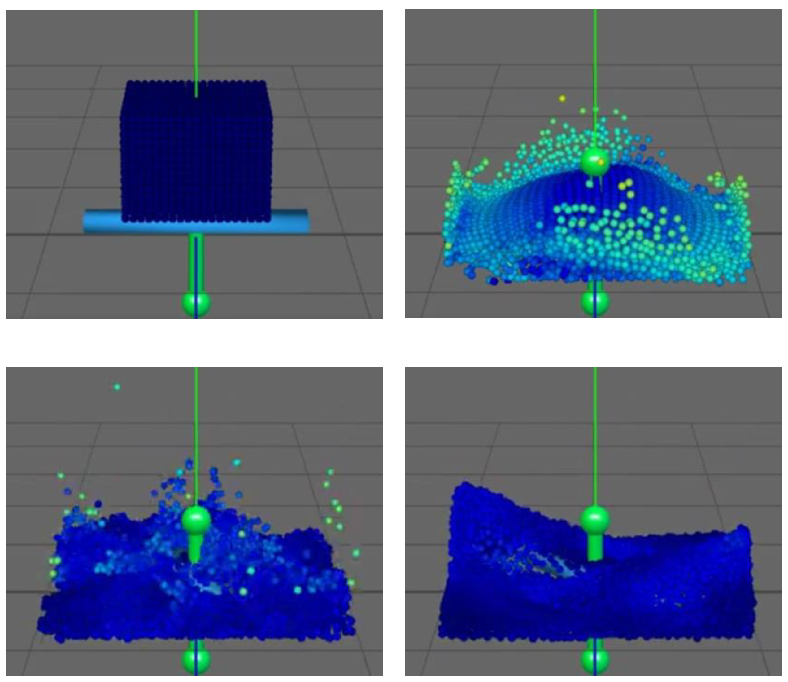
Our third dataset is a simulation of the agitator case with 5054 fluid particles and 200 time steps, as shown in Figure 8. In this case, particles fall out of the air, and there is a paddle at the bottom that alternately moves clockwise and anticlockwise. At the beginning, the paddle rotates clockwise by 30 degrees, and later, its rotation angle of each movement turns to 60 degrees. Importantly, the experiment mainly displays vortex features in the front of rotation path, top and both ends of the paddle. In Figure 9a, the red line at the center of paddle is the rotation invariant axis.

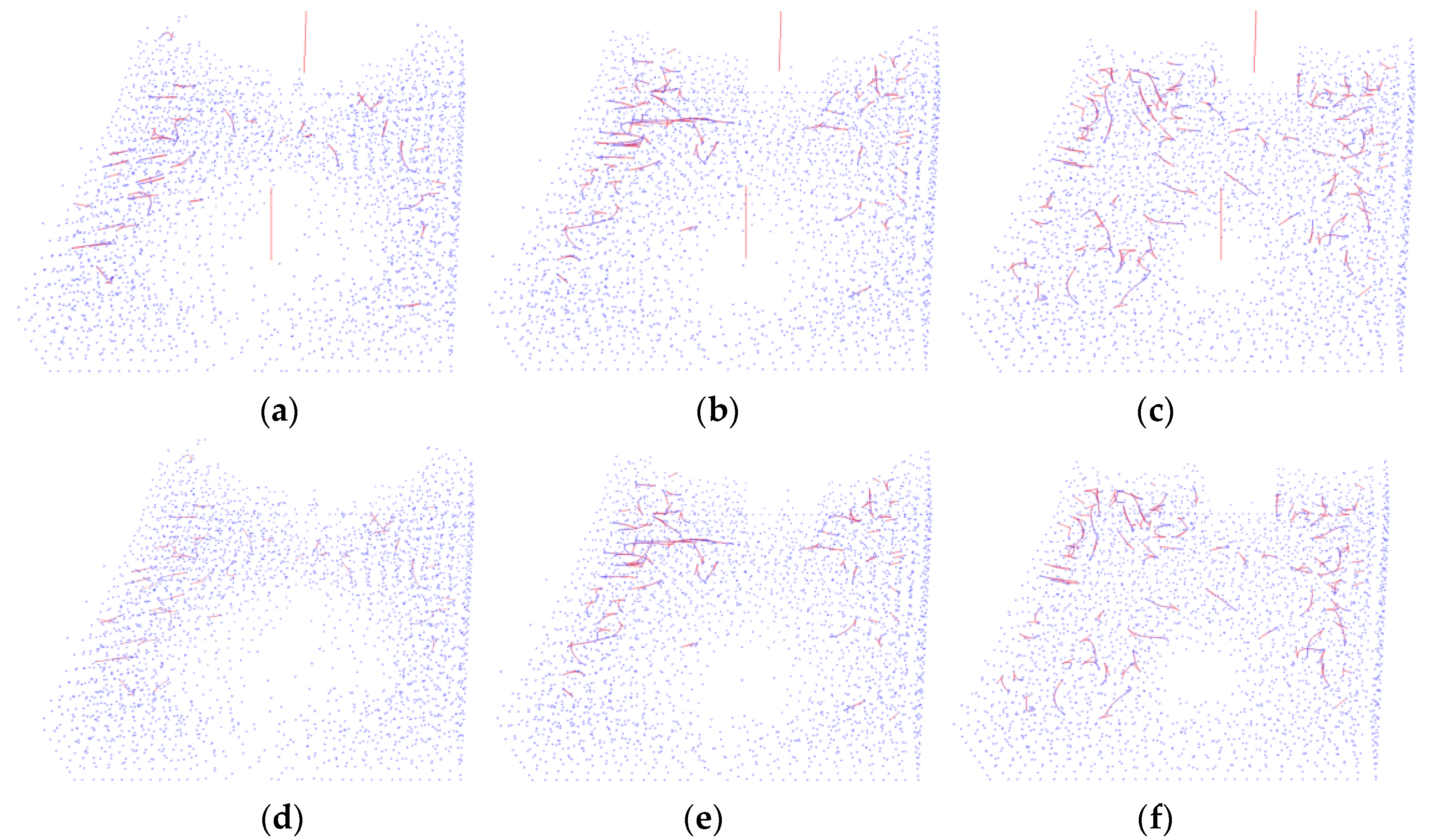
The fourth test data set is SPH simulation of the falling movement of spheres, which is described as follows. It has 3174 particles and 400 time steps. There are two spheres of the same size above a cuboid tank with fluid, which fall into the cuboid tank at the same time. The results of vortex core line extraction are shown in Figure 10.

There are two spheres fall off in this experiment, so we divide the data set into two parts and extract vortex core lines respectively. From the data set, we know the coordinates of the center of the spheres when they fall. Then, we make a red line along the z-axis in three-dimensional space at the center of each sphere as the axis of rotation invariance. Rotation center of these spheres are connected and the middle point between them is taken as the segmentation point of data set. At this point, the data set is divided into two parts by a plane composed of the perpendicular bisector of two spheres and a red line parallel to the z-axis.

The experiment shows vortex features in following regions:

• The left and right sides of two spheres;
• The region between two spheres;
• The region closes to fluid boundary.

According to Figure 10, the extraction results of our multi-axis scene rotation invariant predictor-corrector method are similar to the original predictor-corrector method, which can ensure the accuracy. At present, we simply seek data set segmentation plane at the midpoint of two axes. Obviously, this method ignores many factors, such as vortex intensity. In the future, we will discuss how to segment the data set more reasonably. A more effective method is to calculate the segmentation plane based on vortex strength or direction of fluid, but this will undoubtedly increase the amount of calculation.

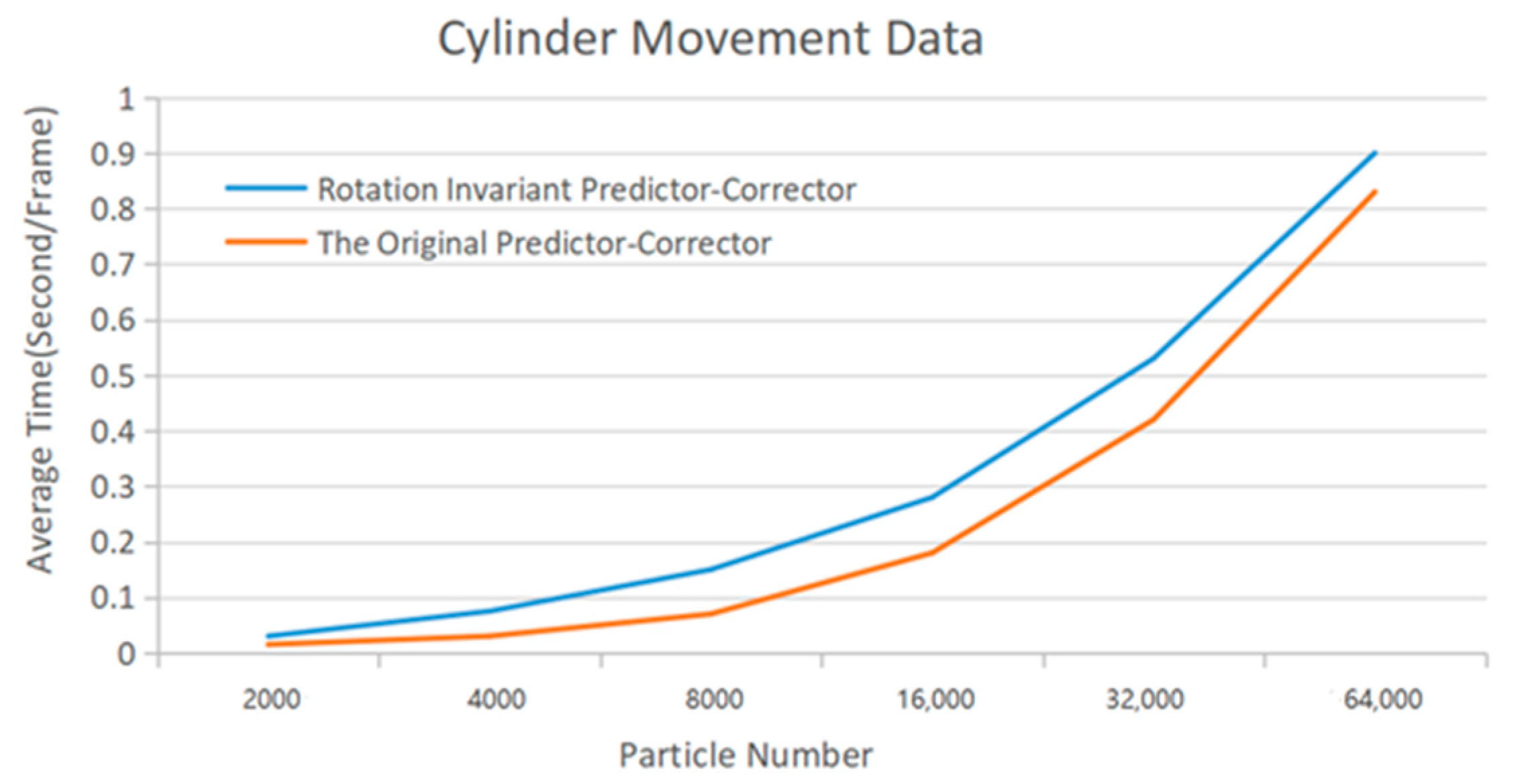
In terms of performance, compared with the original predictor-corrector method, we have made several improvements. Firstly, in order to reduce the computing time of Jacobian, the neighborhood of SPH particles is set to 1.5 times the particle radius, so that neighborhood range is kept minimum and reliable. In addition, the consistent grid is used to improve the performance of searching neighborhood particles. Secondly, when calculating the rotation invariant Jacobian, an additional correction term must be calculated, which slightly increases the calculated amount. Finally, the work of calculating rotation invariant axes and segmenting data set is carried out in pre-treatment, and performance of formal calculation is not reduced. The overall performance of our method is slightly lower than that of the original method, but when the particle number in the data set increases gradually, the performance difference between the two methods becomes smaller, mainly for the following two reasons:

• When the particle number increases, the number of seed points increases much less than that of non-seed points, the proportion of filtering time of non-seed points in the total time increases gradually, and the proportion of computing time of rotation invariant Jacobian decreases.
• In our method, the criterion of seed points is whether the rotation invariant Jacobian has virtual eigenvalues or not, instead of using the general Jacobian to calculate, which makes the steps of extracting seed points stricter and the number of seed points is less than that of the original method. As a result, the calculation times of rotation invariant Jacobian are much less than that of the original method in the prediction and correction steps.

Therefore, with the increase of the particle number, the proportion of the time of filtering non seed points in the total time increases gradually, and the proportion of the calculation time of rotation invariant Jacobian in the total time decreases.

For the cylinder movement data, we set six levels of particle number to calculate the average time of each frame. As can be seen clearly in Figure 11, with the increase of the particle number, the performance of our method tends to the original method.

In the future, we will seek an appropriate data set, which is used to confirm rotation invariance to improve the accuracy of predictor-corrector method under movement of the reference frame. Furthermore, we will investigate the rotation invariant predictor-corrector method on the GPU to promote performance.

5. Conclusions

Above all, it comes to a conclusion that the current study is equipped with two strengths. On the one hand, it modified the predictor-corrector method to adapt to the reference frame which performs any type of movement. In general, there are two types of scenes. In the first kind of scene, there is only one rotation axis, rotation invariance can be used directly. And the second kind of scene is a complex scene with multiple rotation axes, whose data set is divided, and rotation axes and vortex core lines are calculated separately.

On the other hand, the modified predictor-corrector method is applied to rotation invariance, which reduces the influence of the frame that performs rotation on the accuracy of results. The calculation of rotation axis and data set segmentation are carried out in pretreatment procedures, and the results are directly brought into the formal process of vortex extraction. We modify several steps of the original method. Compared with the original predictor-corrector method, the noise of our method is less, and the contour of the feature area is more obvious; in terms of performance, although the overall performance is slightly lower than the original method, the performance of our method tends to the original method in the data with large particle number.

Nevertheless, since the rotation invariant predictor-corrector method has divided the vortex extraction into smaller parts, such as the calculation of seed points, and prediction and correction steps by using rotation invariance, which inevitably inherits problems of the line-based method. One of the problems is that the vortex core line is over segmented, which makes it impossible to accurately present the direction and strength of vortex even if seed points are accurately calculated. In the present study, the possible factors of breaking up vortex core line are reduced. The only basis for judging seed points and correction points relies on that the rotation invariant Jacobian has imaginary eigenvalues. More importantly, the constraint of parallel vector field and the prediction and correction steps should be appropriately decreased to ensure the output quality of vortex core line.

In the future, the authors will mainly improve the method from the following aspects.

First of all, when selecting the axis, the subjectivity should be reduced as much as possible, and a method will be examined to directly extract the axis from the data set. Secondly, when the data set has multiple axes, it is necessary to propose a intelligent method for segmenting it. Thirdly, there is a phenomenon that vortex core lines are sheltered from each other, and adaptive processing will be used in areas with higher density of vortex features.