A Model Predictive Control with Preview-Follower Theory Algorithm for Trajectory Tracking Control in Autonomous Vehicles

Abstract

Research on trajectory tracking is crucial for the development of autonomous vehicles. This paper presents a trajectory tracking scheme by utilizing model predictive control (MPC) and preview-follower theory (PFT), which includes a reference generation module and a MPC controller. The reference generation module could calculate reference lateral acceleration at the preview point by PFT to update state variables, and generate a reference yaw rate in each prediction point. Since the preview range is increased, PFT makes the calculation of yaw rate more accurate. Through physical constraints, the MPC controller can achieve the best tracking of the reference path. The MPC problem is formulated as a linear time-varying (LTV) MPC controller to achieve a predictive model from nonlinear vehicle dynamics to continuous online linearization. The MPC-PFT controller method performs well by increasing the effective length of the reference path. Compared with MPC and PFT controllers, the effectiveness and robustness of the proposed method are proved by simulations of two typical working conditions.

1. Introduction

Due to the worldwide sustained growth in the number of vehicles, it is urgent to reduce traffic accidents caused by the improper operation of the driver and to make the road safe [1]. With the rapid development of electro-control technology and the burgeoning demand for vehicle active safety functions, autonomous vehicles are recognized as a priority for development of the automobile industry in future. For autonomous vehicles, the most important problem to be solved is how to control the vehicle to follow the desired path. Visual servo control, sliding mode control, fuzzy control, linear quadratic regulator (LQR), and model predictive control (MPC) are used for trajectory tracking [2,3,4,5,6]. Although there are many investigations of trajectory tracking, the steering control is still a challenging area involving how to balance vehicle lateral stability and tracking accuracy.

Based on the driver–vehicle–road closed-loop system, driver model is the most critical crux related to the performance of trajectory tracking. It was proposed that a driver model using optimal preview control is a useful and direct method for representing closed-loop automobile driving by CC. Macadam [7]. Preview-follower theory (PFT) was brought forward by K. Guo and P.S. Fancher for modeling the behavior of drivers in the tracking process [8]. The theory describes that the driver’s operation in a path tracking system is always aimed at stabilizing a vehicle along a desired path. R.S. Sharp proposed an autonomous vehicle steering mathematical model based on linear optimal discrete time preview control theory [9]. On the basis of PFT and the error elimination algorithm (EEA), an analytical method in driver modeling was presented to establish a directional control driver model with efficiency, accuracy and driver preference by K. Guo et al. [10]. Additionally, Ding et al. discussed the preview optimal artificial neural network (POSANN) driver model which improved from PFT and EEA applied to arbitrary path following at varying vehicle speed, and J. Cao et al. established a new POSANN driver model taking into consideration jerky dynamics and tracing error between the real track and the planned path [11,12]. S. R. Liu proposed a steering control strategy on the basis of improved preview follower, which avoids the path curvature caused by excessive road traffic and improves the accuracy of steering control strategy [13]. Based on the vehicle dynamics and the preview follower theory. S. Zhang [14] established a lateral preview deviation dynamics model of a vehicle system to deal with parameters perturbations and external disturbances, which improved the accuracy of the trajectory tracking control. G Huang [15] investigated an adaptivity-enhanced path tracking system (AEPTS), which achieved preview distance adaptivity by a dynamic multipoint preview model (DMPPM), and was proved to realize the path tracking with high accuracy at high speeds.

In recent years, model predictive control (MPC) is coming into sight. The idea appearing in MPC is basically [16,17]:

(1)

Predicting the process output at a finite control horizon on account of past and current values;

(2)

Calculating a control sequence by the optimizer taking into account the cost function and the constraints;

(3)

Taking the first control actions at each moment, and repeating the procedure in a receding horizon.

Compared with other control methods, MPC has superiority in trajectory tracking, as it can handle both ‘soft’ and hard constraints on the state variables and control input/output in a multivariable control framework, which improves the performance and achieves the stability. B. Ren [18] proposed a MPC controller, which focused on yaw stability control of in-wheel-motored electric vehicle (EV). C. E. Beal et al. utilized a model predictive envelope controller to binding the vehicle motion within the stable region of the state space defined by estimations of the vehicle sideslip and the tire–road friction coefficient [19,20]. To prevent the infeasible solution of the MPC trajectory tracking controller under strict constraints, a linear MPC with softening constraints path tracking control strategy is proposed by H. Ye [21]. K. Zhang [22] proposed an adaptive learning model predictive control (ALMPC) scheme with a robustness constraint to handle parametric and additive uncertainties in trajectory tracking control. A tube-based robust Model Predictive Control (MPC) approach considering strict constraints in the control signal and the lateral path following error was presented by S. Mata [23]. Based on a defined enveloped stable zone utilizing the friction limits of both the front and rear tires, S. E. Li [24] proposed a linear predictive lateral control method to stabilize a vehicle when tracking a tight desired path at a high speed even on a low-adhesion road. L. Tang [25] discussed a cascaded controller using the kinematic MPC to handle the disturbances on road curvature, which has been conducted to validate the robustness against sensor disturbances and time lag.

The MPC calculations are repeated at each time step and only the first actions are taken, which is a prodigious challenge for real-time capability [26]. It may compromise accuracy of the trajectory tracking or stability of the controlled plant that uses short prediction and control horizons or simple prediction model for favoring fast calculations. In this regard, Paolo Falcone et al. adopted a higher efficiency nonlinear optimal solver [27]. F. Borrelli, P. Falcone et al. [19,28] discussed a MPC controller, which was applied to stabilize a vehicle along a desired path while fulfilling its physical constraints, and relied on the MPC formulation used in the MPC controller mentioned above. P Falcone et al. [29] presented two combined MPC controllers based on vehicle models with different complexities, which concluded that the controller of a simpler vehicle model is not able to stabilize the vehicle at high entry speeds. B. Kim et al. showed a MPC having dual prediction horizons to reduce the length of prediction horizon and obtain the optimal solution rapidly [30]. S. Lee et al. [3,31] proposed a proximate model predictive control (PMPC) and a multilevel approximate model predictive control (MAMPC) to realize the lateral control of the autonomous vehicle and reduce computation load by warm-start online optimization. Based on an autoregressive with exogenous input (ARX) vehicle model, J. Wu [32] proposed an adaptive model predictive control (AMPC) scheme for direct yaw moment control (DYC), which can generate a smoother yaw rate signal with the computational time reduced by half.

The main contributions of this paper are proposing a new MPC scheme combining PFT for increasing reference trajectory range with no increase in computation, which can improve vehicle lateral stability and following accuracy during path following. Based on the above scheme, the process of following the desired path is finally achieved by controlling the front steering wheel angle calculated by the MPC-PFT controller. In order to verify the superiority of the MPC-PFT controller, this paper attempts to compare three different controllers: PFT, MPC and MPC-PFT. The CarSim and MATLAB/Simulink joint simulation method was used. The effectiveness of MPC-PFT control method is proved by simulation analysis of path tracking under typical conditions.

The paper is organized as follows: Section 2 introduces nonlinear vehicle dynamic model used for LTV MPC controller design. Strategy of the MPC-PFT controller and solution on LTV MPC are described in Section 3. In order to verify the proposed controller, two maneuver simulation results are provided in Section 4. Finally, conclusions are summarized in Section 5.

2. Vehicle Dynamics Modeling for Predictive Model of MPC

In this study, a mathematical model of the vehicle should be derived to design the path tracking controllers. We describe the vehicle model considering dynamics aspects in inertial coordinate system. Previous studies implementing MPC controllers based on vehicle models with different complexities have shown that simulations are very time consuming and the tuning is difficult due to more complex vehicle models [29]. Additionally, the target of this research is how to track the desired trajectory fast and steadily, which belongs to the vehicle handling stability, hence a simplified ‘bicycle’ model with a linear tire model is used in this paper.

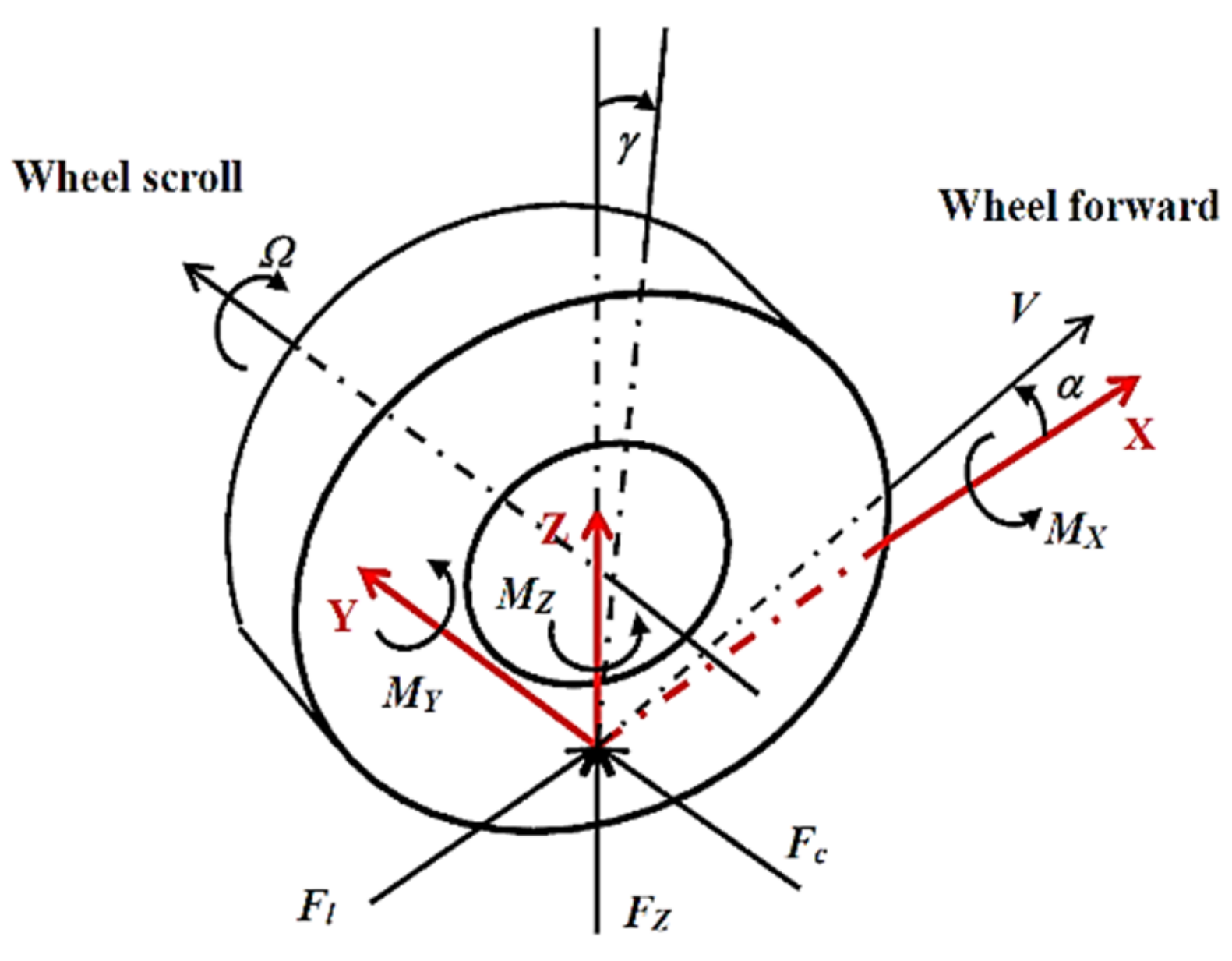
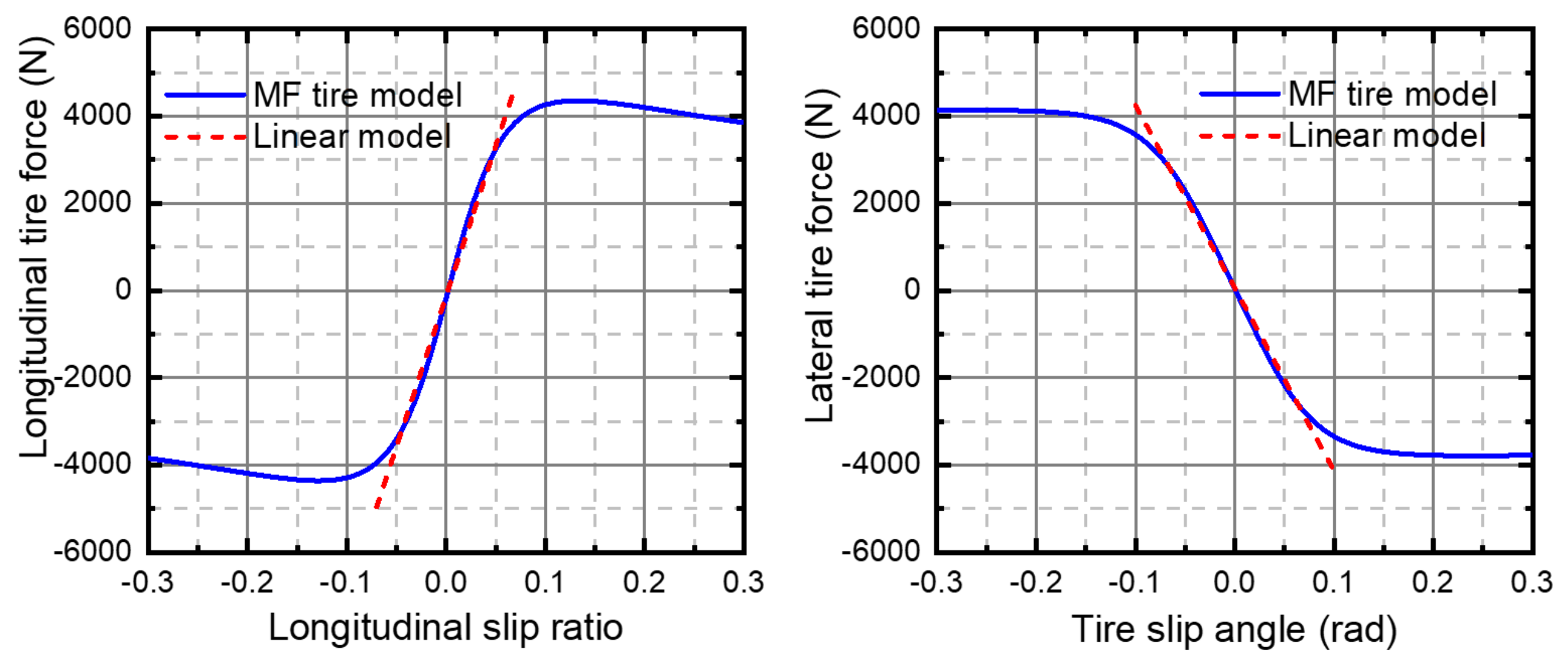
2.1. Linear Tire Model

As the mechanical properties of tires exert measurable effect on vehicle handling stability, as shown in Figure 1, a tire model is essential to establish the vehicle dynamics model and design the control strategy. Generally speaking, a tire model falls into three main categories due to the differential modeling methods: empirical tire model; semiempirical tire model; theoretical tire model. Most of the tire models are too complicated to design the MPC controller, so simplification of the tire model is a crucial issue.

Tire forces can be expressed by:

$$F_l=f_l\left(\alpha ,s,\mu ,F_z\right), F_c=f_c\left(\alpha ,s,\mu ,F_z\right).$$

(1)

where $F_l$ and $F_c$ are the longitudinal and the cornering of the tire force, $\alpha$ stands for the tire slip angle, $s$ denotes the longitudinal slip ratio, μ denotes the road friction coefficient, $F_z$ is the vertical load, $f_l$ and $f_c$ are complex functions of $\alpha$, $s$, $\mu$, and $F_z$.

On the basis of magic formula (MF), H. B. Pacejka provided an empirical tire model fitted to the experimental data by the combination formula of the trigonometric function [33,34], which is widely recognized.

As shown in Figure 2, the lateral tire force and the longitudinal tire force is modeled by the MF tire model. When both the slip angle and the slip ratio are restricted to have small values, the tire model can be considered a linear model:

$$F_l=C_{l}s,F_c=C_{\alpha }\alpha ,$$

(2)

where $C_l$ and $C_{\alpha }$ are the longitudinal and the cornering of the tire stiffness coefficient, respectively.

In Figure 3, $x$ denotes horizontal axis of vehicle coordinate system, ${\delta }_f$ stands for the steering angle for front wheel, $F_{yr}$ and $F_{xr}$ are the lateral force and the longitudinal force for the rear tire, $u_1$ is the speed at the midpoint of the front axle, $u_2$ is the speed at the midpoint of the rear axle. The front tire slip angle ${\alpha }_f$ and rear tire slip angle ${\alpha }_r$ are related to the movement parameters of the vehicle. In Figure 3, ${\alpha }_f$ and ${\alpha }_r$ can be written as:

$${\alpha }_f={\delta }_f-\frac{\dot{y}+a\dot{\phi }}{\dot{x}},{\alpha }_r=-\frac{\dot{y}+b\dot{\phi }}{\dot{x}}.$$

(3)

where $\phi$ is defined as the vehicle yaw angle. Additionally, the system parameters a and b are the distance from center of gravity (COG) to the front axle and from the COG to the rear axle; x and y are the longitudinal displacement and the lateral displacement of COG of the vehicle.

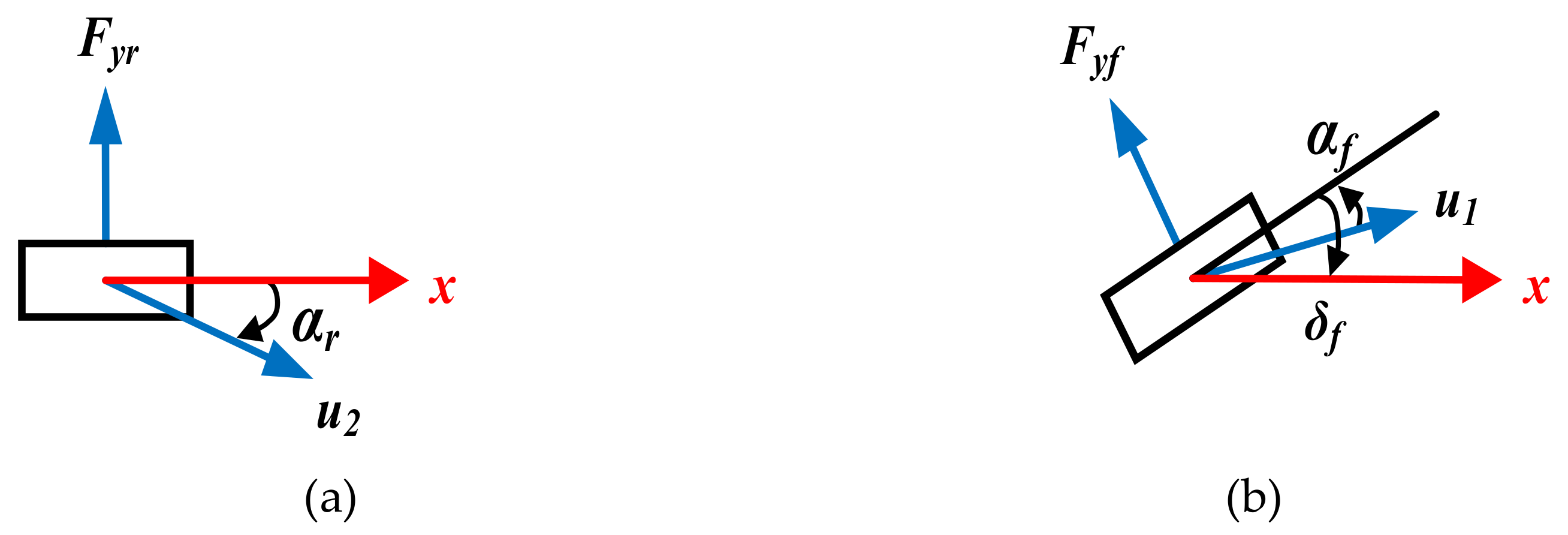
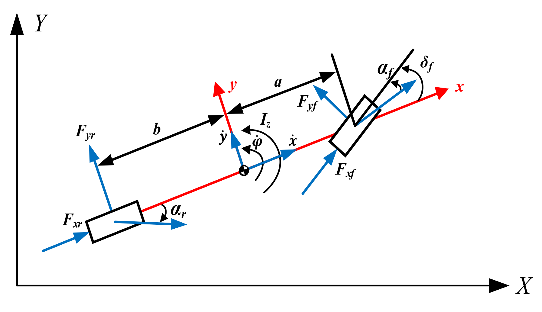
2.2. Vehicle Dynamics Model

Figure 4 illustrates the schematic of a simplified ‘bicycle’ model based on the following simplification [35,36]. Our hypotheses are as follows:

(1)

Lumping the left and right tires together at the front and rear wheel axels.

(2)

Controlling the front wheel angle only.

(3)

Traveling at a constant longitudinal velocity.

The equilibrium equations for a vehicle’s longitudinal, lateral, and yaw movement under the vehicle coordinates can be written by applying Newton’s second law of motion as follows:

$$\left\{\begin{array}{c}m{a}_y=2F_{yf}cos{\delta }_f+2F_{yr}+2F_{xf}sin{\delta }_f\hfill \\ m{a}_x=2F_{xf}cos{\delta }_f+2F_{xr}+2F_{yf}sin{\delta }_f\hfill \\ I_z\ddot{\phi }=2a{F}_{yf}cos{\delta }_f+2a{F}_{xf}sin{\delta }_f-2b{F}_{yr}\hfill \end{array}\right..$$

(4)

where ${\delta }_f$, $\ddot{\phi }$, m, and $I_z$ are the steering angle for front wheel, the vehicle yaw rate acceleration, mass of the vehicle, and the vehicle moment of inertia around the Z-axis. a_y and $a_x$ are the lateral and the longitudinal acceleration of COG of the vehicle along the Y-axis and the X-axis, respectively. $F_{yf}$ and $F_{xf}$ are the lateral and the longitudinal force for the front tire, and $F_{yr}$ and $F_{xr}$ are the lateral force and the longitudinal force for the rear tire.

As the translation and the rotation occur simultaneously during steering, the lateral acceleration a_y and the longitudinal acceleration $a_x$ both consist of two parts

$$a_y=\ddot{y}+\dot{x}\dot{\phi },a_x=\ddot{x}-\dot{y}\dot{\phi }.$$

(5)

The reference trajectory is given in inertial coordinate system, while the vehicle dynamics model is established in the vehicle coordinate system. Transformations among two coordinate systems are determined as follows:

$$\left\{\begin{array}{c}\dot{Y}=\dot{x}sin\phi +\dot{y}cos\phi , \hfill \\ \dot{X}=\dot{x}cos\phi -\dot{y}sin\phi .\hfill \end{array}\right.$$

(6)

where X and Y are the longitudinal and the lateral position in inertial coordinate system, respectively.

3. Design of Control Strategy Basing on MPC-PFT

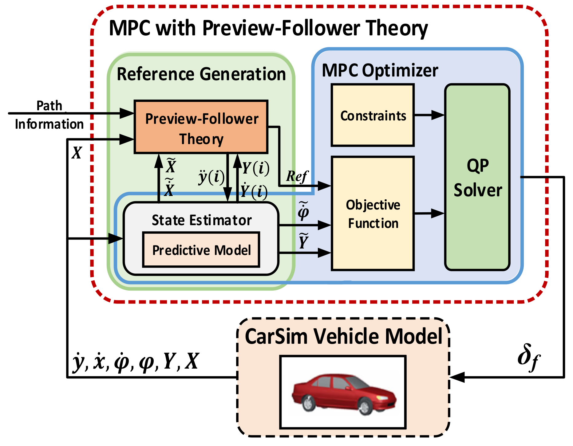
3.1. Overview of the MPC-PFT Theory

Figure 5 shows the association of MPC and PFT, where t represents the current time, X and Y are the longitudinal and the lateral position in the inertial coordinate system, p and T denote the prediction horizon of MPC and the preview time of PFT, respectively. Based on the MPC theory, state variables are predicted at each sample point during a prediction horizon. Combining the predicted vehicle speed and the optimal preview curvature determined by using the PFT with the predicted state variable, the reference yaw rate is derived on every sampling point. Figure 5 shows that in a prediction horizon, the red line represents the reference path which is followed by PFT, and the blue line represents the reference path of the MPC. The reference yaw rate can be calculated by the red line outside the MPC prediction horizon and the reference lateral displacement is shown by the blue line. The reference yaw rate and the reference lateral displacement are executed simultaneously as the set-point for designing the MPC optimizer. Figure 5 demonstrates a metonymical approach towards expanding the effective reference trajectory range in the original basis. On the premise of few additional calculations, the vehicle lateral stability and the following accuracy during the path following can be improved by increasing the length of the effective reference path.

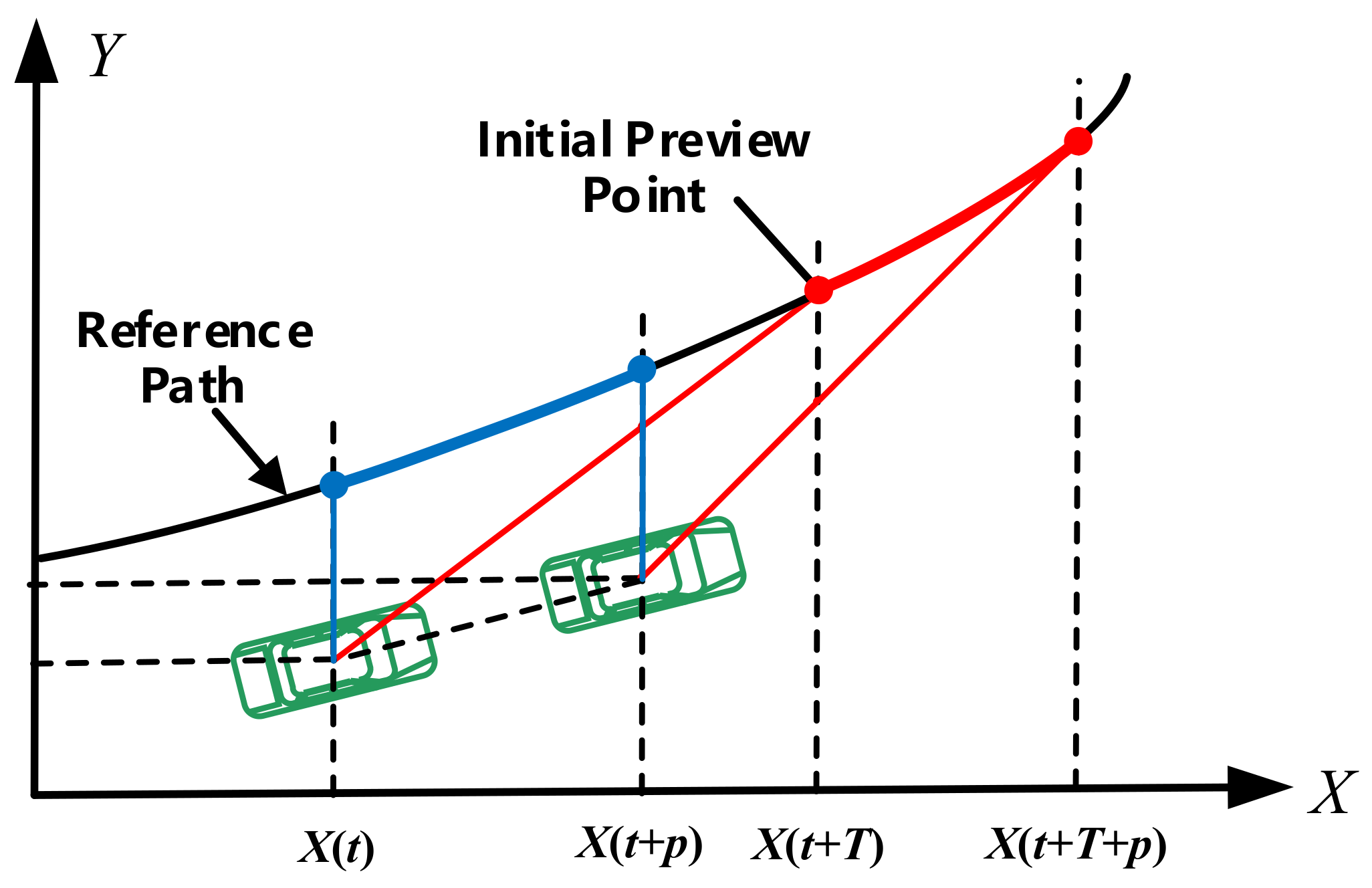
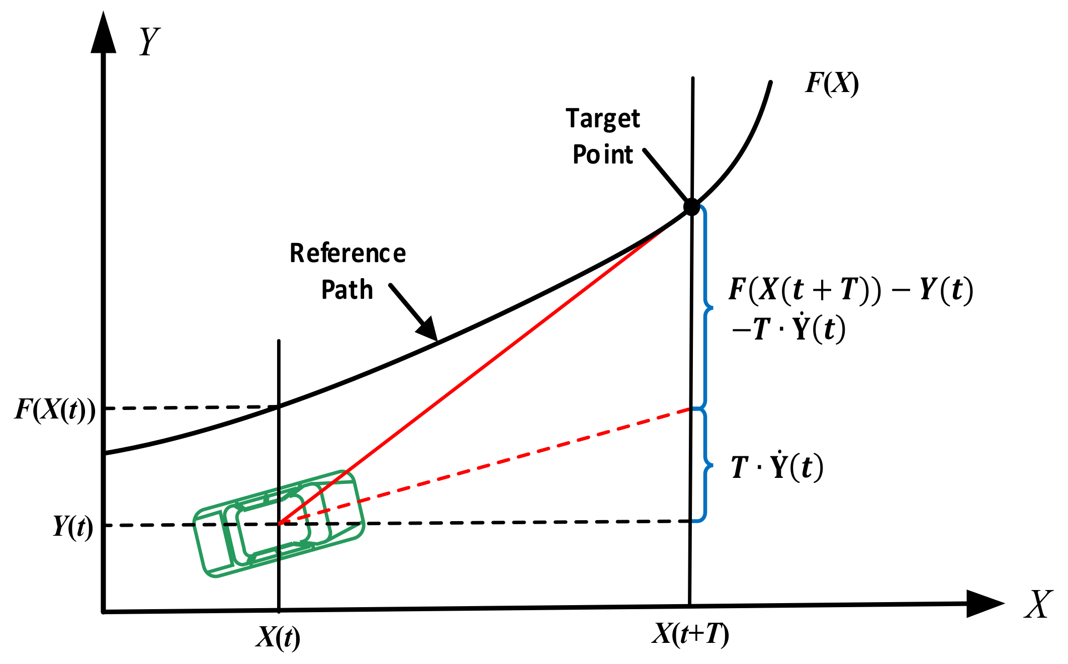
3.2. Preview Follower Theory

In this section, PFT [37] is presented tersely. The movement of the vehicle adheres to the principle of Ackerman mechanism:

$$\ddot{y}=\frac{V^2}{R}.$$

(7)

where R and V stand for the radius of the road curvature and the speed of the vehicle.

In Figure 6, F(X) is the equation of the reference path and at time t, and vehicle states are $y=Y\left(t\right)$ and $\dot{y}=\dot{Y}\left(t\right)$. We indicate that the driver’s preview distance is d, and the preview time is $T=d/V$. The steering angle reaches the target point expressed as $F\left(X\left(t+T\right)\right)$ determined by the trajectory curvature $1/R$ and lateral acceleration $\ddot{Y}\left(t\right)$. After the time T, the lateral displacement of the vehicle can be described as follows:

$$Y\left(t+T\right)=Y\left(t\right)+T\dot{Y}\left(t\right)+\frac{T^2}{2}\ddot{Y}\left(t\right).$$

(8)

The optimal trajectory curvature and lateral acceleration are expected for aligning the lateral displacement $Y\left(t+T\right)$ with the target point $F\left(X\left(t+T\right)\right)$:

$$\begin{array}{c}{\ddot{y}}^{*}\left(t\right)=\frac{2}{T^2}\left[F\left(X\left(t+T\right)\right)-Y\left(t\right)-T\dot{Y}\left(T\right)\right],\\ \frac{1}{R^{*}}=\frac{2}{d^2}\left[F\left(X\left(t+T\right)\right)-Y\left(t\right)-T\dot{Y}\left(T\right)\right].\end{array}$$

(9)

In the vehicle steering process, the yaw rate $\dot{\phi }$ is decided by the vehicle speed and the trajectory curvature:

$$\dot{\phi }=\frac{V}{R^{*}}.$$

(10)

3.3. Strategy of MPC-PFT

3.3.1. Control Scheme of MPC-PFT

The architecture shown in Figure 7 describes the main elements of a path-tracking system using MPC-PFT to determine the front wheel steering angle and the vehicle controller consists of three parts: the reference generation, the MPC optimizer and the CarSim vehicle model. The reference generation module precomputes the reference yaw rate together with the estimated vehicle state. At each sampling time of every prediction horizon, the lateral acceleration calculated by PET will change the estimated vehicle state at next sampling time. Then, the changed state variables at next sampling time will produce a new optimal preview lateral acceleration, thus the reference yaw rate is calculated by the repeatable process of obtaining the optimal preview lateral acceleration and predicting vehicle states. In other words, the state estimation completes at one time in general MPC, but once PFT is applied, the lateral vehicle speed and acceleration will be changed at the next sample time, hence the rolling computation is indispensable for reducing the accumulating error and procuring more accurate reference yaw rate. The reference is composed of two modules: the reference lateral displacement and the reference yaw rate. The reference lateral displacement is derived from the reference path in the predictive horizon while the reference yaw rate is developed by the desired trajectory in the preview distance superimposed on the predictive horizon. Compared with the general MPC, this system extends the length of the effective reference path without extra calculation burden. The MPC optimizer with input and output constraints computes the steering wheel angle in order to follow the reference path, and the solution of MPC-PFT joint control algorithm with constraints is transformed into a quadratic programming problem with constraints.

3.3.2. Reference Trajectory Generation

The variable $r\left(k+i\right)={\left[{\dot{\phi }}_{ref}\left(k+i\right),Y_{ref}\left(k+i\right)\right]}^T$ denotes the reference trajectory at the time $k+i$ based on the information available at time k. $Y_{ref} \left(k+i\right)$ is the desired path at the time $k+i$ and ${\dot{\phi }}_{ref}\left(k+i\right)$ is calculated by PFT. The method of obtaining the reference yaw rate is described in Algorithm 1.

Algorithm 1 Reference yaw rate generation

Input: Vehicle longitudinal speed, lateral speed, longitudinal position, and lateral position at the time k are denoted by $v_x\left(k\right)$, $v_y\left(k\right)$, $X\left(k\right)$, and $Y\left(k\right)$. Output: Vehicle reference yaw rate ${\dot{\phi }}_{ref}$ at the time k. Repeat until getting Np reference point, or $i = Np+1$. Step 1: State estimator: generate $X\left(k+i\right)$ via $X\left(k+i\right)=X\left(k\right)+v_x\left(k\right)*i*t$, where $t$ is the sample time, $i$ represents the $i-\mathrm{th}$ prediction point. Step 2: Update: $v_y\left(k+i\right)$ and $Y\left(k+i\right)$ by $v_y\left(k+i\right)=v_y\left(k+i-1\right)+{\ddot{y}}_{ref}\left(k+i-1\right)*T$ and $Y\left(k+i\right)=v_y\left(k+i-1\right)*T+0.5*{\ddot{y}}_{ref}\left(k+i-1\right)*T^2$. Step 3: Preview-Follower Theory: obtain ${\ddot{y}}_{ref}\left(k+i\right)$ and ${\dot{\phi }}_{ref}\left(k+i\right)$ by optimal preview driver model: ${\ddot{y}}_{ref}\left(k+i\right)=\frac{2}{T^2}\left[F\left(X\left(k+i\right)\right)-Y\left(k+i\right)-T\dot{Y}\left(k+i\right)\right],$ ${\dot{\phi }}_{ref}\left(k+i\right)=\frac{V}{R^{*}}=\frac{2V}{d^2}\left[F\left(X\left(k+i\right)\right)-Y\left(k+i\right)-T\dot{Y}\left(k+i\right)\right],$ where ${\ddot{y}}_{ref}\left(k+i\right)$ and ${\dot{\phi }}_{ref}\left(k+i\right)$ are the reference lateral acceleration and yaw rate at the $i-\mathrm{th}$ prediction point, respectively. Step 4: $i=i+1$. End repeat

Based on the preview-follower theory, the reference yaw rate and trajectory are shown as follows:

$$\tilde{\mathit{r}}\left(k\right)=\left[\begin{array}{c}\mathit{r}\left(k+1\right)\\ \mathit{r}\left(k+2\right)\\ ⋮\\ \mathit{r}\left(k+m\right)\\ ⋮\\ \mathit{r}\left(k+N_p\right)\end{array}\right].$$

(11)

3.3.3. Approximation of Linear Time Varying (LTV) Model

The discrete-time state space equation of the nonlinear vehicle dynamics model described by Equations (2)–(6) is developed as follows:

$${\mathit{x}}_{nl}\left(k+1\right)=f_{nl}\left({\mathit{x}}_{nl}\left(k\right),\mathit{u}\left(k\right)\right).$$

(12)

where $i\ge 0$, $f_{nl}\left({\mathit{x}}_{\mathit{n}\mathit{l}}\left(k\right),\mathit{u}\left(k\right)\right)$ represents the state update function of the nonlinear vehicle dynamics model, ${\mathit{x}}_{\mathit{n}\mathit{l}}$ is the state, the control input $\mathit{u}$ is the front steering angle. The significant theory of the linearization method obtains the part linear pattern behind the series expansion at the work-point [38,39]. Equation (12) at the state ${\mathit{x}}_0\left(k\right)$ and input ${\mathit{u}}_0$ can be linearized as:

$$\overline{\mathit{x}}\left(k+1\right)={\mathit{A}}_0\left(k\right)\overline{\mathit{x}}\left(k\right)+{\mathit{B}}_0\left(k\right)\overline{\mathit{u}}\left(k\right).$$

(13)

where:

$$\overline{\mathit{x}}\left(k\right)=\mathit{x}\left(k\right)-{\mathit{x}}_0\left(k\right),\overline{\mathit{u}}\left(k\right)=\mathit{u}\left(k\right)-{\mathit{u}}_0,$$

(14)

$${\mathit{A}}_0\left(i\right)={\left.\frac{\partial f_{nl}}{\partial \mathit{x}}\right|}_{\begin{array}{c}{x}_0\left(i\right)\\ {\mathit{u}}_0\end{array}},{\mathit{B}}_0\left(i\right)={\left.\frac{\partial f_{nl}}{\partial \mathit{u}}\right|}_{\begin{array}{c}{x}_0\left(i\right)\\ {\mathit{u}}_0\end{array}},$$

(15)

At the prediction point $i$, the LTV system can be rewritten as:

$$\begin{array}{c}\mathit{x}\left(k+i+1\right)={\mathit{A}}_i\left(k\right)x\left(k+i\right)+{\mathit{B}}_{i,k}u\left(k+i\right)+{\mathit{e}}_i\left(k+i\right),\\ \mathit{y}\left(k\right)=\mathit{C}\mathit{x}\left(k+1\right).\end{array}$$

(16)

where $\mathit{x}={\left[\dot{y}, \dot{x}, \dot{\phi }, \phi , Y, X\right]}^T$ is the state vector, $\mathit{u}={\delta }_f$ is the control input, $\mathit{C}={\left[0 0 1 0 0;0 0 0 0 1 0\right]}^T$, and $\mathit{y}={\left[\dot{\phi }, Y\right]}^T$ is the state output.

In a prediction horizon, $\mathit{A}i\left(k\right), \mathit{B}i\left(k\right), \mathit{x}\left(k+i\right), \mathit{e}\left(k+i\right)$, and $\mathit{u}\left(k+i\right)$ are updated at each time i. In order to simplify calculation, assuming that

$$\begin{array}{c}\mathit{x}\left(k+i\right)=\mathit{x}\left(k\right),i=1,\dots ,N_p-1,\\ \mathit{u}\left(k+i\right)=\mathit{u}\left(k\right),i=1,\dots ,N_c-1,\\ {\mathit{A}}_i\left(k\right)=\mathit{A}={\left.\frac{\partial f_{nl}}{\partial \mathit{x}}\right|}_{\begin{array}{c}\mathit{x}\left(k\right)\\ \mathit{u}\left(k\right)\end{array}},i=1,\dots ,N_p-1.\\ {\mathit{B}}_i\left(k\right)=\mathit{B}={\left.\frac{\partial f_{nl}}{\partial \mathit{u}}\right|}_{\begin{array}{c}\mathit{x}\left(k\right)\\ u\left(k\right)\end{array}},i=1,\dots ,N_p-1,\\ \mathit{e}\left(k+i\right)=\mathit{e}\left(k\right)=\mathit{x}\left(k+1\right)-{\mathit{A}}_i\left(k\right)\mathit{x}\left(k\right)-{\mathit{B}}_i\left(k\right)\mathit{u}\left(k\right),i=1,\dots ,N_p-1.\end{array}$$

(17)

where N_p and N_c are called the prediction horizon and the control horizon.

Since the model input is the control increment Δu(t) instead of the control signal u(t), an incremental state space model [17,40] is derived as follows:

$$\begin{array}{c}\stackrel{{\mathit{x}}_m\left(k+1\right)}{\overbrace{\left[\begin{array}{c}\mathit{x}\left(k+1\right)\\ \mathit{u}\left(k\right)\end{array}\right]}}=\stackrel{{\mathit{A}}_m}{\overbrace{\left[\begin{array}{cc}\mathit{A}& \mathit{B}\\ 0& \mathit{I}\end{array}\right]}}\stackrel{{\mathit{x}}_m\left(k\right)}{\overbrace{\left[\begin{array}{c}\mathit{x}\left(k\right)\\ \mathit{u}\left(k-1\right)\end{array}\right]}}+\stackrel{{\mathit{B}}_m}{\overbrace{\left[\begin{array}{c}\mathit{B}\\ \mathit{I}\end{array}\right]}}\Delta \mathit{u}\left(k\right)+\stackrel{{\mathit{G}}_m}{\overbrace{\left[\begin{array}{c}\mathit{I}\\ 0\end{array}\right]}}\mathit{e}\left(k\right),\\ \mathit{y}\left(k\right)=\stackrel{{\mathit{C}}_m}{\overbrace{\left[\begin{array}{cc}\mathit{C}& 0\end{array}\right]}}\left[\begin{array}{c}\mathit{x}\left(k\right)\\ \mathit{u}\left(k-1\right)\end{array}\right].\end{array}$$

(18)

The general form of Equation (18) is given by:

$$\begin{array}{c}{\mathit{x}}_m\left(k+1\right)={\mathit{A}}_m{\mathit{x}}_m\left(k\right)+{\mathit{B}}_m\Delta \mathit{u}\left(k\right)+{\mathit{G}}_m\mathit{e}\left(k\right),\\ \mathit{y}\left(k\right)={\mathit{C}}_m{\mathit{x}}_m\left(k\right).\end{array}$$

(19)

for the sake of reducing computational burden, the change of lateral dynamic caused by PFT is neglected. At the sampling instant k, k > 0, the future vehicle states, the future state variables, and the future control movements formulated in terms of current state variable information x(k) are denoted by [41]:

$$\tilde{\mathit{y}}\left(k\right)=\left[\begin{array}{c}\mathit{y}\left(k+1\right)\\ \mathit{y}\left(k+2\right)\\ ⋮\\ \mathit{y}\left(k+m\right)\\ ⋮\\ \mathit{y}\left(k+N_p\right)\end{array}\right],\Delta \tilde{\mathit{u}}\left(k\right)=\left[\begin{array}{c}\Delta \mathit{u}\left(k\right)\\ \Delta \mathit{u}\left(k+1\right)\\ ⋮\\ \Delta \mathit{u}\left(k+N_c+1\right)\end{array}\right],\tilde{\mathit{e}}\left(k\right)=\left[\begin{array}{c}\mathit{e}\left(k\right)\\ \mathit{e}\left(k+1\right)\\ ⋮\\ \mathit{e}\left(k+m\right)\\ ⋮\\ \mathit{e}\left(k+N_p-1\right)\end{array}\right].$$

(20)

From Equation (19), the output prediction is described by:

$$\tilde{\mathit{y}}\left(k\right)=\mathit{F}{\mathit{x}}_m\left(k\right)+\mathit{\Phi }\Delta \tilde{\mathit{u}}\left(k\right)+\mathit{\Theta }\tilde{\mathit{e}}\left(k\right).$$

(21)

where:

$$\begin{array}{c}\mathit{F}=\left[\begin{array}{c}{\mathit{C}}_m{\mathit{A}}_m\\ {\mathit{C}}_m{\mathit{A}}_m{}^2\\ {\mathit{C}}_m{\mathit{A}}_m{}^3\\ ⋮\\ {\mathit{C}}_m{\mathit{A}}_m{}^{Np}\end{array}\right],\\ \mathit{\Phi }=\left[\begin{array}{ccccc}{\mathit{C}}_m{\mathit{B}}_m& 0& 0& \cdots & 0\\ {\mathit{C}}_m{\mathit{A}}_m{\mathit{B}}_m& {\mathit{C}}_m{\mathit{B}}_m& 0& \cdots & 0\\ {\mathit{C}}_m{\mathit{A}}_m{}^2{\mathit{B}}_m& {\mathit{C}}_m{\mathit{A}}_m{\mathit{B}}_m& {\mathit{C}}_m{\mathit{B}}_m& \cdots & 0\\ ⋮& ⋮& ⋮& \ddots & ⋮\\ {\mathit{C}}_m{\mathit{A}}_m{}^{N_p-1}{\mathit{B}}_m& {\mathit{C}}_m{\mathit{A}}_m{}^{N_p-2}{\mathit{B}}_m& {\mathit{C}}_m{\mathit{A}}_m{}^{N_p-3}{\mathit{B}}_m& \cdots & {\mathit{C}}_m{\mathit{A}}_m{}^{N_p-N_c}{\mathit{B}}_m\end{array}\right]\\ \mathit{\Theta }=\left[\begin{array}{ccccc}{\mathit{C}}_m{\mathit{G}}_m& 0& 0& \cdots & 0\\ {\mathit{C}}_m{\mathit{A}}_m{\mathit{G}}_m& {\mathit{C}}_m{\mathit{G}}_m& 0& \cdots & 0\\ {\mathit{C}}_m{\mathit{A}}_m{}^2{\mathit{G}}_m& {\mathit{C}}_m{\mathit{A}}_m{\mathit{G}}_m& {\mathit{C}}_m{\mathit{G}}_m& \cdots & 0\\ ⋮& ⋮& ⋮& \ddots & ⋮\\ {\mathit{C}}_m{\mathit{A}}_m{}^{N_p-1}{\mathit{G}}_m& {\mathit{C}}_m{\mathit{A}}_m{}^{N_p-2}{\mathit{G}}_m& {\mathit{C}}_m{\mathit{A}}_m{}^{N_p-3}{\mathit{G}}_m& \cdots & {\mathit{C}}_m{\mathit{G}}_m\end{array}\right]\end{array}$$

(22)

3.3.4. Formulation and Calculation of MPC Problem

The primary objective of the controller is to determine the sequence of control moves that will minimize the sum of the squared deviations of the predicted output from the reference trajectory. The objective function J is:

$$J\left(k\right)={\left(\tilde{\mathit{r}}\left(k\right)-\tilde{\mathit{y}}\left(k\right)\right)}^T\mathit{Q}\left(\tilde{\mathit{r}}\left(k\right)-\tilde{\mathit{y}}\left(k\right)\right)+\Delta {\tilde{\mathit{u}}}^T\left(k\right)\mathit{R}\Delta \tilde{\mathit{u}}\left(k\right)+\rho {\epsilon }^2.$$

(23)

where Q, R represent weight matrices, ρ is the weight coefficient, ε is the relaxing factor. In Equation (23), the first term brings the predicted output as close as possible to the reference signal, while the second term is linked to consider a direct limiting of the control increment Δu, and the third term is desired for preventing emerging the infeasible solution during execution.

With taking into account the constrained condition relaxation, it was more suitable for the optimization of trajectory tracking with the driver’s operation. Thus, the constraints are expressed as:

$$\left\{\begin{array}{c}\Delta {\mathit{u}}_{\min }\le \Delta \mathit{u}\le \Delta {\mathit{u}}_{\max }\\ {\mathit{u}}_{\min }\le \mathit{u}\le {\mathit{u}}_{\max }\\ {\mathit{Y}}_{\min }\le \mathit{Y}\le {\mathit{Y}}_{\max }\\ 0\le \epsilon \le M\end{array}\right..$$

(24)

The constraints as the inequalities with linear-in-the-parameter $\Delta \tilde{\mathit{u}}$ are:

$$\begin{gathered} \left[\begin{array}{c}-{\mathit{I}}_m\\ {\mathit{I}}_m\end{array}\right]\Delta \tilde{\mathit{u}}\le \left[\begin{array}{c}-\Delta {\tilde{\mathit{u}}}_{\min }\\ \Delta {\tilde{\mathit{u}}}_{\max }\end{array}\right], \\ \left[\begin{array}{c}-{\mathit{C}}_2\\ {\mathit{C}}_2\end{array}\right]\Delta \tilde{\mathit{u}}\le \left[\begin{array}{c}-{\tilde{\mathit{u}}}_{\min }+{\mathit{C}}_1\mathit{u}\left(k-1\right)\\ {\tilde{\mathit{u}}}_{\max }-{\mathit{C}}_1\mathit{u}\left(k-1\right)\end{array}\right], \end{gathered}$$

(25)

where:

$${\mathit{C}}_1={\left[\begin{array}{c}{\mathit{I}}_m\\ {\mathit{I}}_m\\ {\mathit{I}}_m\\ ⋮\\ {\mathit{I}}_m\end{array}\right]}_{m{N}_c\times m},{\mathit{C}}_2={\left[\begin{array}{ccccc}{\mathit{I}}_m& 0_m& 0_m& \cdots & 0_m\\ {\mathit{I}}_m& {\mathit{I}}_m& 0_m& \cdots & 0_m\\ {\mathit{I}}_m& {\mathit{I}}_m& {\mathit{I}}_m& \cdots & 0_m\\ ⋮& ⋮& ⋮& \ddots & ⋮\\ {\mathit{I}}_m& {\mathit{I}}_m& {\mathit{I}}_m& \cdots & {\mathit{I}}_m\end{array}\right]}_{m{N}_c\times m{N}_c},$$

(26)

$$\left[\begin{array}{c}-\mathit{\Phi }\\ \mathit{\Phi }\end{array}\right]\Delta \tilde{\mathit{u}}\le \left[\begin{array}{c}-{\tilde{\mathit{Y}}}_{\min }+\mathit{F}{\mathit{x}}_m\left(k\right)\\ {\tilde{\mathit{Y}}}_{\max }-\mathit{F}{\mathit{x}}_m\left(k\right)\end{array}\right].$$

(27)

where m is the dimension of control input.

The constrained MPC for tracking problem can be casted into solving the quadratic programming (QP) problem which has been extensively studied, and the objective function J and the constraints are described as:

$$\begin{array}{c}J=\frac{1}{2}\Delta {\tilde{\mathit{u}}}^T\left(k\right)\mathit{H}\Delta \tilde{\mathit{u}}\left(k\right)+\Delta {\tilde{\mathit{u}}}^T\mathit{b},\\ \mathit{M}\Delta \tilde{\mathit{u}}\le \mathit{\Gamma },\\ \Delta {\tilde{\mathit{u}}}_{\min }\le \Delta \tilde{\mathit{u}}\le \Delta {\tilde{\mathit{u}}}_{\max }.\end{array}$$

(28)

where:

$$\begin{array}{c}\mathit{H}={\mathit{\Phi }}^T\mathit{Q}\mathit{\Phi }+\mathit{R},\\ \mathit{b}=\left(\mathit{F}\tilde{\mathit{x}}\left(k\right)+\mathit{\Theta }\mathit{e}-\tilde{\mathit{r}}\left(k\right)\right)\mathit{Q}\mathit{\Phi },\end{array}$$

(29)

$$\mathit{M}=\left[\begin{array}{c}-{\mathit{C}}_2\\ {\mathit{C}}_2\\ -\mathit{\Phi }\\ \mathit{\Phi }\end{array}\right],\mathit{\Gamma }=\left[\begin{array}{c}-{\tilde{\mathit{u}}}_{\min }+{\mathit{C}}_1\mathit{u}\left(k-1\right)\\ {\tilde{\mathit{u}}}_{\max }-{\mathit{C}}_1\mathit{u}\left(k-1\right)\\ -{\tilde{\mathit{Y}}}_{\min }+\mathit{F}{\mathit{x}}_m\left(k\right)\\ {\tilde{\mathit{Y}}}_{\max }-\mathit{F}{\mathit{x}}_m\left(k\right)\end{array}\right].$$

(30)

To prevent over-constraint problems, there are soft constraints on this QP problem:

$$J_{soft}=\frac{1}{2}{\left[\begin{array}{c}\Delta \tilde{\mathit{u}}\left(k\right)\\ \epsilon \end{array}\right]}^T\left[\begin{array}{cc}\mathit{H}& 0_{m{N}_c\times 1}\\ 0_{1\times m{N}_c}& \rho \end{array}\right]\left[\begin{array}{c}\Delta \tilde{\mathit{u}}\left(k\right)\\ \epsilon \end{array}\right]+{\left[\begin{array}{c}\Delta \tilde{\mathit{u}}\\ \epsilon \end{array}\right]}^T\left[\begin{array}{cc}\mathit{b}& 0\end{array}\right],$$

(31)

$$\left[\begin{array}{c}\begin{array}{cc}-{\mathit{C}}_2& 0_{m{N}_c\times 1}\\ {\mathit{C}}_2& 0_{m{N}_c\times 1}\end{array}\\ \begin{array}{cc}-\mathit{\Phi } & 0_{m{N}_y\times 1}\\ \mathit{\Phi }& 0_{m{N}_y\times 1}\end{array}\end{array}\right]\left[\begin{array}{c}\Delta \tilde{\mathit{u}}\\ \epsilon \end{array}\right]\le \Gamma ,$$

(32)

$$\left[\begin{array}{c}\Delta {\tilde{\mathit{u}}}_{\min }\\ 0\end{array}\right]\le \left[\begin{array}{c}\Delta \tilde{\mathit{u}}\\ \epsilon \end{array}\right]\le \left[\begin{array}{c}\Delta {\tilde{\mathit{u}}}_{\max }\\ M\end{array}\right].$$

(33)

By combining Equations (31)–(33), the sequence of the optimal steering commands computed at the time k is:

$$\Delta {\tilde{\mathit{u}}}^{*}\left(k\right)=\left[\Delta {\mathit{u}}^{*}\left(k\right) \Delta {\mathit{u}}^{*}\left(k+1\right) \cdots \Delta u^{*}\left(k+N_c-1\right)\right]{ }^T.$$

(34)

As it is a receding horizon strategy, only the first vector Δu*(k) of $\Delta {\tilde{\mathit{u}}}^{*}\left(k\right)$ is used, rejecting the rest and repeating the calculations at the next sampling time:

$$u\left(k\right)=u\left(k-1\right)+{\left[\stackrel{N_c}{\overbrace{\begin{array}{cc}{\mathit{I}}_m& \begin{array}{ccc}{0}_m& \dots & 0_m\end{array}\end{array}}}\right]}^T\Delta {\tilde{\mathit{u}}}^{*}\left(k\right).$$

(35)

4. Simulation Results and Analysis

In this section, using Matlab/Simulink and CarSim joint simulation, through two representative experiments, comparative simulations on the proposed controller were performed to evaluate the effectiveness of the controller. CarSim is a proven professional simulation software whose vehicle model is highly accurate. The vehicle model of CarSim is embedded as a Simulink S-function while the MPC-PFT controller is also coded in S-function.

Two other kinds of controllers were used to indicate the validation of MPC-PFT control algorithm, which are the MPC controller and PFT controller. Vehicle parameters are identical with an E-class Sedan in CARSIM selected as the subject vehicle and some main parameters of the controllers are listed in

Table 1. Part of the main parameters of the controller.

Parameter	Value	Units
$T_s$	0.02	-
$N_p$	30	-
$N_c$	12	-
$u_{max}$	25	deg
$u_{min}$	−25	deg
$\Delta {\mathrm{u}}_{\max }$	0.5	deg
$\Delta {\mathrm{u}}_{\min }$	−0.5	deg

.

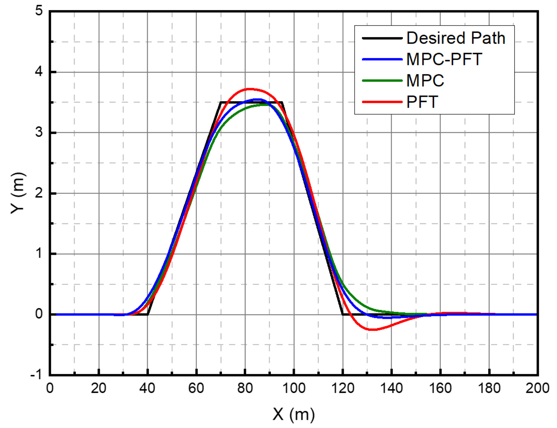
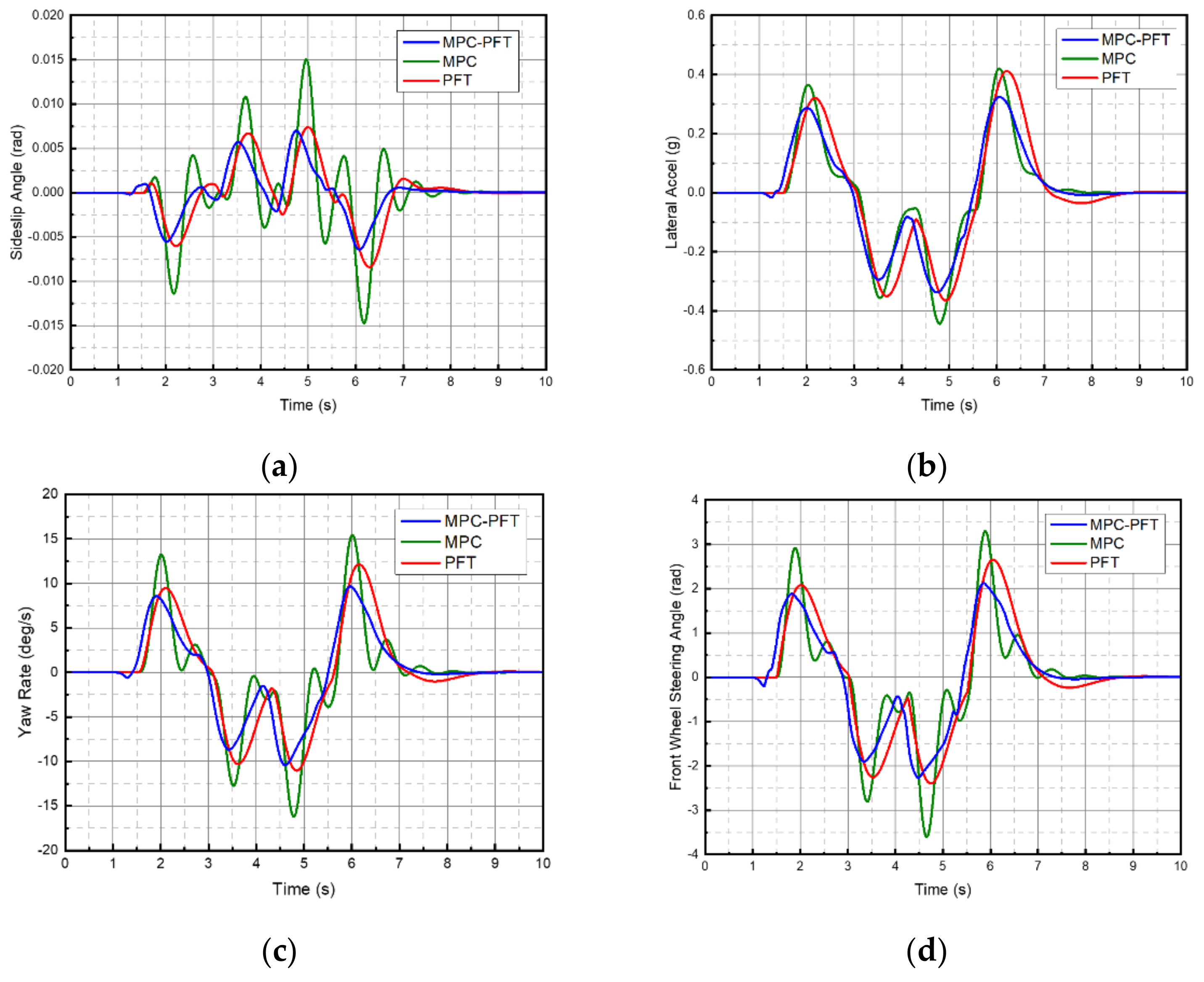
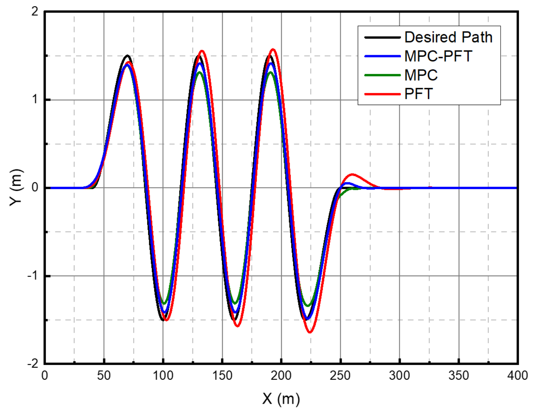
4.1. Double Lane Change (DLC) Maneuver

The test scenario is a DLC maneuver, with the vehicle traveling at 20 m/s. The road trajectory of the controlled vehicle is shown in Figure 8. Since the yaw rate, the lateral acceleration and the sideslip angle are crucial factors for the stability of vehicle lateral dynamics, simulation results of the three states are presented in Figure 9a–c, the front wheel steering angle calculated in each controller is presented in Figure 9d.

In Figure 8, it can be seen that MPC-PFT has a quicker response than the MPC controller and better tracking performance than the PFT controller. In Figure 9a, the sideslip angle of MPC controller behaves badly, and the MPC-PFT controller is superior to the PFT controller from amplitude, reaction speed and stability. Although there is no wide gap between those three controllers on lateral acceleration shown in Figure 9b, the MPC-PFT controller also plays a better role in rapidity and stability. Figure 9c illustrates the vehicle yaw rate, and the results show that both PFT and MPC-PFT controllers have a good stability performance, the numerical value of the yaw rate from the MPC-PFT controller is smaller. Actually, the tracking accuracy and the handling stability are in conflict in a critical situation such as a DLC maneuver [42]. Through expanding prediction horizon by PFT, the MPC-PFT controller combines advantages with the tracking performance of the MPC controller and the handling performance of the PFT controller. The MPC-PFT controller solves the conflict mentioned above.

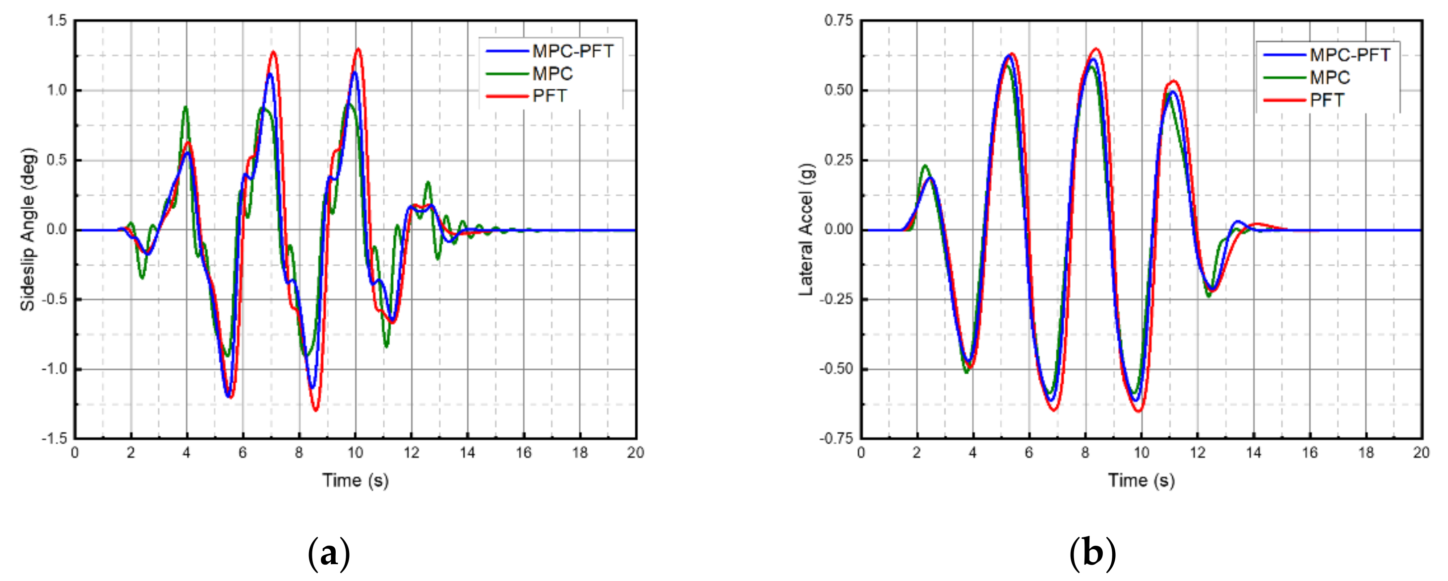
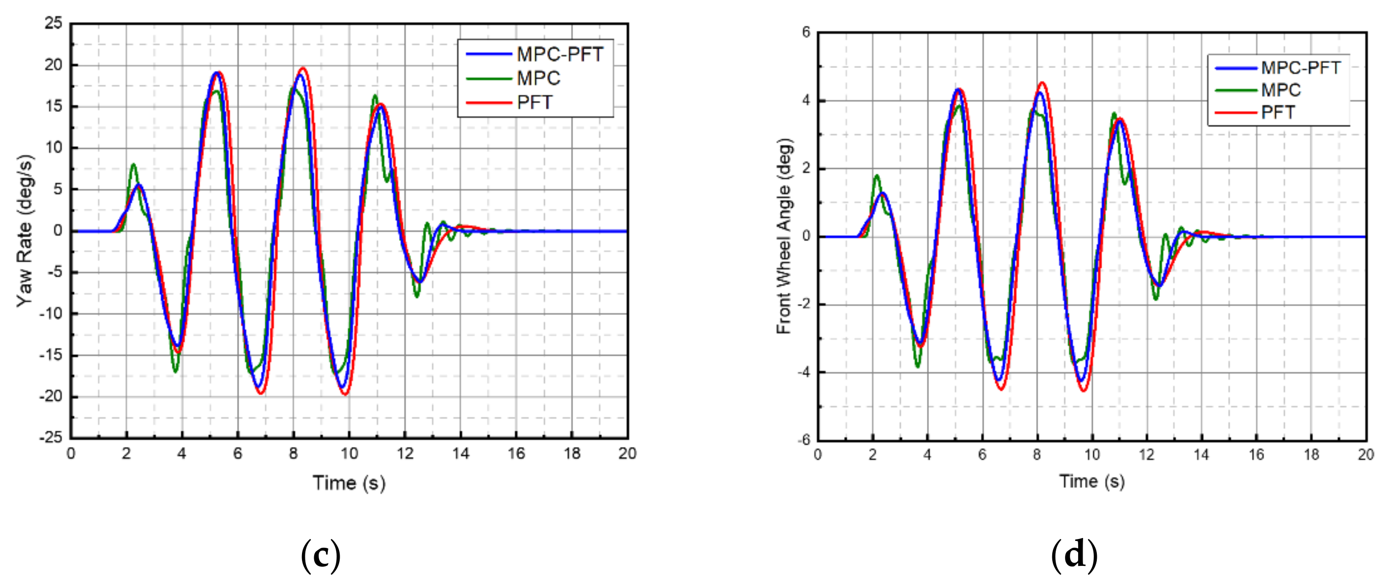
4.2. Slalom Maneuver

This scenario is a slalom maneuver. We assume that the longitudinal speed is 20 m/s. Figure 10 and Figure 11 show the simulation results of each state of MPC, MPC-PFT and PFT controllers, respectively. Simulation results of the path that controlled vehicles travel, the sideslip angle, the lateral acceleration, and the yaw rate are presented in Figure 10 and Figure 11a–c, the front wheel steering angle calculated in each controller is presented in Figure 11d.

It can be seen from these simulation results that MPC controller performs badly under extreme conditions like a slalom maneuver. Figure 10 shows the trajectory of the vehicle, indicating that the tracking performance of the MPC controller is poor, while the tracking error and delay of the PFT controller are gradually increasing. In Figure 11a, although the sideslip angle of the MPC controller is smaller than other two controllers, it is not stable. Figure 11a illustrates that the MPC-PFT controller is more stable than the PFT controller. In Figure 11b, all of three controllers perform well in lateral acceleration while the MPC controller is not stable enough in the first and last curve, and the lateral acceleration of the PFT controller is bigger than the MPC and MPC-PFT controllers. The yaw rate and the front wheel angle of MPC controller are also not stable as shown in Figure 11c,d, and the yaw rate amplitude of the PFT controller is bigger than the other two controllers, so its stability is not good.

In Figure 10, it shows that compared with the PFT controller, the MPC-PFT controller runs rapidly and has significant advantages in tracking performance and stability.

5. Conclusions and Future Work

In order to improve the tracking accuracy and lateral stability, a new control scheme by combining MPC and PFT was presented to realize the path tracking of autonomous vehicles. In which, PFT was used to design a MPC controller, and LTV MPC was used to continuously online linearize the nonlinear vehicle dynamics model. We obtained the reference yaw rate which was used to form the reference trajectory of LTV MPC controller by PFT in a prediction horizon. The advantages of this control scheme are that the length of effective reference path can be increased within an invariable prediction horizon. In order to verify the MPC-PFT control algorithm, the contrast simulations of MPC and PFT controllers were completed. Simulation results of the different conditions showed the effectiveness and robustness of the MPC-PFT controller. The MPC-PFT controller has better tracking performance and handling performance than the MPC and PFT controllers due to the increase in length of effective reference path.

The performance of the MPC-PFT algorithm was verified by the joint simulation method of CarSim and MATLAB/Simulink. In the future, an online MPC-PFT controller for path tracking should be built. Combined with the research of the longitudinal control methods, we are going to apply the MPC-PFT scheme in a collision avoidance system and finally apply it to a real car.

References

1. World Health Organization. Global Status Report on Road Safety 2015; World Health Organization: Geneva, Switzerland, 2015. [Google Scholar]
2. Han, Y.; Cheng, Y.; Xu, G. Trajectory tracking control of AGV based on sliding mode control with the improved reaching law. IEEE Access 2019, 7, 20748–20755. [Google Scholar] [CrossRef]
3. Lee, S.H.; Lee, Y.O.; Kim, B.A. Proximate model predictive control strategy for autonomous vehicle lateral control. In Proceedings of the 2012 American Control Conference (ACC), Montreal, QC, Canada, 27–29 June 2012; pp. 3605–3610. [Google Scholar]
4. Yan, F.; Li, B.; Shi, W.; Wang, D. Hybrid visual servo trajectory tracking of wheeled mobile robots. IEEE Access 2018, 6, 24291–24298. [Google Scholar] [CrossRef]
5. Peng, S.; Shi, W. Adaptive fuzzy output feedback control of a nonholonomic wheeled mobile robot. IEEE Access 2018, 6, 43414–43424. [Google Scholar] [CrossRef]
6. Levinson, J.; Askeland, J.; Becker, J. Towards fully autonomous driving: Systems and algorithms. In Proceedings of the 2011 IEEE Intelligent Vehicles Symposium (IV), Baden-Baden, Germany, 5–9 June 2011; pp. 163–168. [Google Scholar]
7. MacAdam, C.C. Application of an optimal preview control for simulation of closed-loop automobile driving. IEEE Trans. Syst. Man Cyber. 1981, 11, 393–399. [Google Scholar] [CrossRef]
8. Guo, K.; Fancher, P. Preview-Follower method for modelling closed-loop vehicle directional control. In Proceedings of the Nineteenth Annual Conference on Manual Control, Cambridge, MA, USA, 1 January 1983. [Google Scholar]
9. Sharp, R.; Casanova, D.; Symonds, P. A mathematical model for driver steering control with design tuning and performance results. Veh. Syst. Dyn. 2000, 33, 289–326. [Google Scholar]
10. Guo, K.; Cheng, Y.; Ding, Y. Analytical method for modeling driver in vehicle directional control. Veh. Syst. Dyn. 2004, 41, 401–410. [Google Scholar]
11. Ding, H.; Guo, K.; Wan, F. An analytical driver model for arbitrary path following at varying vehicle speed. Veh. Syst. Dyn. 2008, 5, 204–218. [Google Scholar] [CrossRef]
12. Cao, J.; Lu, H.; Guo, K.; Zhang, J. A driver modeling based on the preview-follower theory and the jerky dynamics. Math. Prob. Eng. 2013, 2013. [Google Scholar] [CrossRef]
13. Liu, S. The improved algorithm to preview follower control applied research on intelligent electric vehicle. Adv. Mater. Res. 2015, 1079, 1022–1025. [Google Scholar] [CrossRef]
14. Zhang, S.; Zhao, X.; Zhu, G.; Shi, P.; Hao, Y.; Kong, L. Adaptive trajectory tracking control strategy of intelligent vehicle. Int. J. Distrib. Sens. Netw. 2020, 16, 1550147720916988. [Google Scholar] [CrossRef]
15. Huang, G.; Yuan, X.; Shi, K.; Liu, Z.; Wu, X. Adaptivity-Enhanced path tracking system for autonomous vehicles at high speeds. IEEE trans. Intell. Transp. Syst. 2020, 5, 626–634. [Google Scholar] [CrossRef]
16. Richalet, J.; Rault, A.; Testud, J. Model predictive heuristic control. Automatica 1978, 14, 413–428. [Google Scholar] [CrossRef]
17. Camacho, E.F.; Bordons, E. Model predictive control. Int. J. Robust Nonlin. 2008, 18, 799–810. [Google Scholar]
18. Ren, B.; Chen, H.; Zhao, H.; Yuan, L. MPC-Based yaw stability control in in-wheel-motored EV via active front steering and motor torque distribution. Mechatronics 2016, 38, 103–114. [Google Scholar] [CrossRef]
19. Borrelli, F.; Falcone, P.; Keviczky, T. MPC-Based approach to active steering for autonomous vehicle systems. IJVAS 2005, 3, 265–291. [Google Scholar] [CrossRef]
20. Beal, C.; Gerdes, J. Model predictive control for vehicle stabilization at the limits of handling. IEEE Trans. Control Sys. Tech. 2013, 21, 1258–1269. [Google Scholar] [CrossRef]
21. Ye, H.; Jiang, H.; Ma, S. Linear model predictive control of automatic parking path tracking with soft constraints. Int. J. Adv. Robot. Syst. 2019, 16, 1729881419852201. [Google Scholar] [CrossRef] [Green Version]
22. Zhang, K.; Sun, Q.; Shi, Y. Trajectory tracking control of autonomous ground vehicles using adaptive learning MPC. IEEE Trans. Neural Netw. Learn. Syst. 2021, 1–11. [Google Scholar] [CrossRef]
23. Zubizarreta, A.; Pinto, C. Robust tube-based model predictive control for lateral path tracking. IEEE trans. Intell. Transp. Syst. 2019, 4, 569–577. [Google Scholar]
24. Li, S.E.; Chen, H.; Li, R. Predictive lateral control to stabilise highly automated vehicles at tire-road friction limits. Veh. Syst. Dyn. 2020, 58, 768–786. [Google Scholar] [CrossRef]
25. Tang, L.; Yan, F.; Zou, B. An improved kinematic model predictive control for high-speed path tracking of autonomous vehicles. IEEE Access 2020, 8, 51400–51413. [Google Scholar] [CrossRef]
26. Sharp, R.; Peng, H. Vehicle dynamics applications of optimal control theory. Veh. Syst. Dyn. 2011, 49, 1073–1111. [Google Scholar] [CrossRef]
27. Falcone, P.; Borrelli, F.; Asgari, J. Towards Real-time model predictive control approach for autonomous active steering. In Proceedings of the 6th International Symposium on Advanced Vehicle Control, Taipei, Taiwan, 20–24 August 2006; pp. 599–604. [Google Scholar]
28. Falcone, P.; Borrelli, F.; Asgari, J.; Tseng, H.E.; Hrovat, D. Predictive active steering control for autonomous vehicle systems. IEEE Trans. Control Syst. Tech. 2007, 15, 566–580. [Google Scholar] [CrossRef]
29. Falcone, P.; Tseng, H.; Borrelli, F.; Asgari, J.; Hrovat, D. MPC-Based yaw and lateral stabilisation via active front steering and braking. Veh. Syst. Dyn. 2008, 46, 611–628. [Google Scholar] [CrossRef]
30. Kim, B.; Son, Y.; Lee, S. Model predictive control using dual prediction horizons for lateral control. IFAC Proc. Vol. 2013, 46, 280–285. [Google Scholar] [CrossRef]
31. Lee, S.; Chung, C. Multilevel approximate model predictive control and its application to autonomous vehicle active steering. In Proceedings of the 52nd IEEE Conference on Decision and Control, Florence, Italy, 10–13 December 2013; pp. 5746–5751. [Google Scholar]
32. Wu, J.; Wang, Z.; Zhang, L. Unbiased-Estimation-Based and computation-efficient adaptive MPC for four-wheel-independently-actuated electric vehicles. Mech. Mach. Theory 2020, 154, 104100. [Google Scholar] [CrossRef]
33. Pacejka, H.; Bakker, E. The magic formula tyre model. Veh. Syst. Dyn. 1992, 21, 1–18. [Google Scholar] [CrossRef]
34. Doria, A.; Tognazzo, M.; Cusimano, G. Identification of the mechanical properties of bicycle tyres for modelling of bicycle dynamics. Veh. Syst. Dyn. 2013, 51, 405–420. [Google Scholar] [CrossRef]
35. Falcone, P.; Borrelli, F.; Asgari, J. A model predictive control approach for combined braking and steering in autonomous vehicles. In Proceedings of the 2007 Mediterranean Conference on Control & Automation, Athens, Greece, 27–29 June 2007; pp. 1–6. [Google Scholar]
36. Gao, Y. Model predictive control for autonomous and semiautonomous vehicles. Ph.D. Thesis, UC Berkeley, Berkeley, CA, USA, 2014. [Google Scholar]
37. Guo, K. Drivers-Vehicle close-loop simulation of handing by "Preselect Optimal Curvature Method". Auto. Eng. 1984, 3, 1–16. [Google Scholar]
38. Falcone, P.; Borrelli, F.; Tseng, H. Linear time-varying model predictive control and its application to active steering systems: Stability analysis and experimental validation. Int. J. Robust Nonlin. 2007, 18, 862–875. [Google Scholar] [CrossRef]
39. Falcone, P.; Tufo, M.; Borrelli, F. A linear time varying model predictive control approach to the integrated vehicle dynamics control problem in autonomous systems. In Proceedings of the 2007 46th IEEE Conference on Decision and Control, New Orleans, LA, USA, 12–14 December 2007; pp. 2980–2985. [Google Scholar]
40. Maciejowski, J.M. Predictive Control: With Constraints; Pearson Education: London, UK, 2002. [Google Scholar]
41. Wang, L. Model Predictive Control System Design and Implementation Using MATLAB; Springer Science & Business Media: Berlin, Germany, 2009; pp. 25–36. [Google Scholar]
42. Cao, H.; Song, X.; Zhao, S. An optimal model-based trajectory following architecture synthesising the lateral adaptive preview strategy and longitudinal velocity planning for highly automated vehicle. Veh. Syst. Dyn. 2017, 55, 1143–1188. [Google Scholar] [CrossRef]
Figure 1. Tire model.
Symmetry 13 00381 g001
Figure 2. Longitudinal and lateral tire forces.
Symmetry 13 00381 g002
Figure 3. Vehicle slip angle. (a) Rear wheel slip angle. (b) Front wheel slip angle.
Symmetry 13 00381 g003
Figure 4. Vehicle dynamics model.
Symmetry 13 00381 g004
Figure 5. Predictive horizon of combining MPC and preview-follower theory.
Symmetry 13 00381 g005
Figure 6. Preview-follower theory.
Symmetry 13 00381 g006
Figure 7. Control scheme of MPC-PFT.
Symmetry 13 00381 g007
Figure 8. Path following results of DLC maneuver at 20 m/s.
Symmetry 13 00381 g008
Figure 9. Simulation results of DLC maneuver at 20 m/s. (a) Sideslip angle, (b) lateral acceleration results, (c) yaw rate, (d) steering wheel angle results.
Symmetry 13 00381 g009
Figure 10. Path following results of a slalom maneuver at 20 m/s.
Symmetry 13 00381 g010
Figure 11. Simulation results of a slalom maneuver at 20 m/s. (a) Sideslip angle, (b) lateral acceleration results, (c) yaw rate, (d) steering wheel angle results.
Symmetry 13 00381 g011aSymmetry 13 00381 g011b