Abstract
Inspired by the large number of applications for symmetric nonlinear equations, an improved full waveform inversion algorithm is proposed in this paper in order to quantitatively measure the bone density and realize the early diagnosis of osteoporosis. The isotropic elastic wave equation is used to simulate ultrasonic propagation between bone and soft tissue, and the Gauss–Newton algorithm based on symmetric nonlinear equations is applied to solve the optimal solution in the inversion. In addition, the authors use several strategies including the frequency-grid multiscale method, the envelope inversion and the new joint velocity–density inversion to improve the result of conventional full-waveform inversion method. The effects of various inversion settings are also tested to find a balanced way of keeping good accuracy and high computational efficiency. Numerical inversion experiments showed that the improved full waveform inversion (FWI) method proposed in this paper shows superior inversion results as it can detect small velocity–density changes in bones, and the relative error of the numerical model is within 10%. This method can also avoid interference from small amounts of noise and satisfy the high precision requirements for quantitative ultrasound measurements of bone.
1. Introduction
Nowadays, osteoporosis is a major health issue affecting millions of people in the world [1], where the bone mineral density (BMD) measurement is one of kind important determination standards for the objective reflection of reduced bone mass and the evaluation of bone changes [2]. Dual energy X-ray absorptiometry (DXA) utilizes differences in the penetration of different tissues by X-ray to calculate BMD. Although it is simple to operate, and has a short scanning time and high accuracy, the DXA method lacks information about bone structure or bone mechanical performance. Additionally, even though the radiation dose used in DXA is low, multiple uses will cause radiation accumulation [3]. Quantitative computed tomography (QCT) uses the principles of CT imaging and can analyze structural details between the cortical bone and the trabecular bone [4]. High-resolution methods, such as microcomputed tomography and nuclear magnetic resonance imaging, were gradually developed on the foundation of QCT [5,6]. These methods can be used to obtain detailed bone geometric distribution and structural images. However, since they are expensive and have a high radiation dose (around 100 times that of DXA), it is difficult to promote these methods in normal hospitals [7].
Quantitative ultrasound (QUS) is a new technology developed in recent decades as a replacement for X-ray [8,9]. In 1984, Langton et al. [10] firstly proposed the concept of ultrasonic bone measurement. This QUS does not directly measure BMD but uses several parameter values of bone, such as broadband ultrasound attenuation (BUA), speed of sound (SOS), and broadband ultrasound backscatter (BUB). Not only can these parameters laterally reflect BMD, but they are also intimately associated with bone structure and biomechanical properties [11]. Compared to X-ray, the QUS method is inexpensive and does not cause radiation injury, but involves more parameters. Up to now the physical theoretical model is not perfect and the measurement accuracy and application scope need to be further studied [12,13,14].
The full-waveform inversion (FWI) method is a kind of quantitative estimation method of underground media by minimizing the misfit between observational data and simulated data based on the numerical modeling of seismic wave propagation [15]. In recent years, the FWI algorithm has been applied in medical ultrasound image processing [16], especially in the ultrasound tomography algorithm for the chest and other soft tissues [17]. In 2017, Bernard et al. [18] used the FWI algorithm for BMD measurements. However, for simplicity, they only used simple fluid isotropic media and neglected the effect of shear wave propagation inside the bones. In addition, the highest velocity set in their theoretical bone model was only 2600 m/s, which is too low when compared with the propagation velocity of ultrasonic waves in real cortical bone (approximately 3500–4000 m/s). Compared to seismic image processing, using the FWI algorithm in ultrasonic BMD measurements still faces two difficulties: (1) the seismic source is usually 10 Hz to 30 Hz while the frequency of ultrasonic sources is usually above 100 kHz and has higher accuracy requirements for the algorithm; (2) since there are large differences in the propagation velocity of ultrasonic waves in the bones and the surrounding soft tissues, the inversion process tends to fall into the local minimum and generate the cycle-skipping phenomenon.
In this study, we successfully employed the FWI algorithm in the ultrasound quantitative measurement of BMD. This overcomes the difficulties encountered when seismic image inversion is converted to ultrasound image inversion, while retaining the high resolution and high precision of the FWI algorithm. We elaborately designed four objective models to examine the feasibility of our improved full-waveform inversion algorithm in bone quantitative measurement. Furthermore, we consider the media as elastic and isotropic. In traditional UCT algorithms, two-dimensional sections that are perpendicular to the bone central axis are usually chosen for inversion. Therefore, the assumption of isotropy is consistent with the fact that the image plane is perpendicular to the axis of bone. In this paper, we will first introduce the theoretical aspects of this problem and provide solutions to avoid getting trapped into local minimum and the cycle skipping phenomenon. We also discuss how to increase inversion efficiency and improve poor results in density inversion. After a series of numerical experiments, we present that our improved method can be used to accurately obtain the distribution images for the velocity and density of different bone model, with an error below 10% from the objective model. Additionally, good inversion images can still be obtained after the addition of different noise.
2. Theory of the Full-Waveform Inversion Algorithm
With regard to the subject of this study, the basic steps for using the full-waveform algorithm to solve nonlinear inversion problems were as follows: First, the initial model was inputted as the initial model. The forward simulation of the propagation of ultrasonic waves in human tissues was used to obtain the observed numerical records for the initial model at the receiver. The difference between the actual numerical records and the observed numerical records was used as an objective function to modify the parameters of the initial model. After multiple iterations of the aforementioned process, the optimized approximation model for human tissues could be obtained. In general, the full waveform inversion (FWT) algorithm aims to estimate the parameters of elastic medium underground by solving symmetric nonlinear optimization problems that minimize the mismatched energy between modeling data and field data.
2.1. Forward Algorithm
The two-dimensional acoustic equation in the time domain of variable density is shown as follows:
where, represents divergence and is a position parameter, and expressed as a two-dimensional vector in two-dimensional space. is the volume modulus, and the specific form is as follows:
The main numerical techniques for seismic wave field modeling include the finite-element method [19], pseudo-spectral method [20], and finite-difference method [21,22]. Due to its easy implementation and the satisfactory compromise between accuracy and efficiency, the finite-difference method is preferred. For a comprehensive overview of applications of the finite-difference method, see Moczo et al. [23]. Compared to low-order schemes, high-order finite-difference schemes can control this numerical dispersion by using larger grid spacing. In this study, we employed the fourth-order staggered-grid finite-difference method [24].
2.2. Inversion Algorithm
2.2.1. Objective Function
Generally, the physical parameter of the model m can be used to describe the displacement u of forward numerical simulation at the receiver. The relationship between the two can be expressed abstractly in the following nonlinear function:
For every pair of source and receiver, the difference between the observed data and the forward simulation data can be used to calculate the residual:
The norm form of the of the residual vector is defined (i.e., the residual function can also be termed as the objective function). Therefore, the solution of the corresponding model physical parameter m when the objective function takes a minimum is the final solution to the model in the inversion results. The observed data of the r-th receiver in the s-th source is expressed as , and the value of the forward wave field is expressed as ; then, the objective function is as follows:
2.2.2. Least Squares Local Optimization Method
There are many waveform inversion methods (e.g., the steepest descent method [25], conjugate gradient method [26], Gauss–Newton method [27,28], and quasi-Newton method [29]). Most methods require certain constraints and assumptions. Some require good background values, some are only effective for horizontal medium models, and some have excessive iterations and cumbersome calculations, while others are at the theoretical research stage and do not have good numerical simulation results. In this study, the authors used the Gauss–Newton method based on symmetric nonlinear equations combined with regularization and the least squares method for bone quantitative ultrasound imaging. The residual between the forward wave field and the observed data were used for back-propagation in the medium so that the parameter values at every point in the model were corrected through the inversion symmetry. Therefore, a real model can be inversed, even without a priori estimation of the model. This method has good stability and uses a smaller number of iterations compared to gradient methods.
In the time domain, the invisible summation in Equation (5) is based on the number of source and receiver pairs and the number of time samples. This is because, in full-waveform inversion, the amount of data and model parameters involved are large, and local optimization methods are usually used to solve the Equation (5) An example is Equation (6) in which an initial model was defined, and the model was iteratively updated. Assume an updated M × N dimensional model parameter matrix m, which can be written as the summation of the initial model and the perturbation model . In this matrix, M and N represent the number of horizontal and vertical grids of the two-dimensional model, respectively:
By conducting a second-order Taylor–Lagrange expansion of the objective function at the domain and ignoring terms above the second order, we obtain:
where H is an M × N order Hessian second-derivative matrix that defines the curvature of the function at point . The elements in the Hessian matrix are obtained from the following equation:
When the derivative of Equation (9) is set to zero, the following is obtained:
is a matrix with M dimensions. By taking in the above equation, the descent direction of the perturbation model in Equation (9) can be obtained. The method for solving Equation (9) is usually known as Newton’s method. The characteristic of this algorithm is that the front of the gradient is multiplied by the inverse operator of the Hessian matrix, which is comparable to carrying out preprocessing of the gradient and can significantly increase the rate of convergence. However, the disadvantages of Newton’s method are also very significant as it requires calculation of the entire Hessian matrix. When the number of model parameters is relatively large, the amount of observation data will also correspondingly increase. Then, the computational load for the Hessian matrix will become extremely large.
In the Gauss–Newton algorithm, the Hessian operator in Equation (8) is expressed using the approximate Hessian operator , which is a diagonal-dominated matrix. Then the Newton equation Equation (9) can be degenerated into the Gauss–Newton equation:
2.2.3. Gradient
For the elastic wave Equation (1), assuming a perturbations of model parameter cause a perturbation of displacement . Define the adjoint wave field which is adopted by propagating the residual data from the receiver positions backwards through the elastic medium. Then the gradient for Lame parameters , and density can be written as [30]:
Using the chain rule to obtain the corresponding gradient expression for the P-wave velocity, S-wave velocity, and density parameters:
2.2.4. Regularization
It is widely known that full-waveform inversion algorithm is an ill-posed problem, and its solution faces a difficult problem, which is the instability of approximate solutions. The method typically used to solve these problems is to introduce a smoothing functional in the objective function so that instability is avoided by regularization. The following functional substitutions are suitable for this study [31]:
where and are second-order smoothing matrices in the x and z directions, respectively, and and are regular parameters used to determine the proportion of the smoothing function. When Equations (10) and (13) are introduced into the calculation formula for matrix parameters Equation (6), the following equation is obtained:
From this equation, updated images can be obtained through step-by-step Gauss–Newton regularized inversion.
2.3. Improvements on the Full-Waveform Inversion Algorithm
As mentioned in the introduction section, the ultrasound quantitative measurement of bone is more complicated than seismic measurement. First, the source frequency of ultrasound is relatively high, which will make the low-frequency information of inversion inadequate; second, it would be difficult to get good inversion results and easy to fall into local minimum because of the high contrast of parameters between the bone and surrounding soft tissue; third, the bone quantitative measurement is generally applied in clinical, so improving the efficiency of inversion is also necessary. Therefore, we made some improvements to the traditional full-waveform inversion algorithm in order to meet the needs of bone quantitative measurement.
2.3.1. Cycle Skipping
One factor affecting the full-waveform inversion result is the phenomenon of cycle skipping. For nonlinear objective functions, the Born approximation requires the travel time error between the forward-recorded data and the observed data to be smaller than one time period [32]. When the error between the initial model and the real model is relatively large, the cycle skipping will result in the objective function converging to the local minimum.
Prattle et al. expressed the aforementioned conditions using relative time error and the number of propagated wavelengths as follows [33], where represents the total time for forward simulation:
Passing the inversion process through a low-pass filter can prevent cycle skipping. The obtained model can be used as the initial model for the subsequent higher frequency inversion, until the inversion covers the range of all usable frequencies.
According to the difference dispersion condition, large scale of grid can also satisfy the dispersion condition when the low frequency is used, which means that the number of spatial discrete points can be reduced as well as the computational complexity. So the frequency multiscale propagation can be combined with grid multiscale inversion, as shown in Figure 1. The idea of grid multiscale method [34] is to divide the model parameters into several grids of different scales, and the problem is solved sequentially from coarse grids (large scale) to fine grids (small scale). The inversion results for the coarse grid are interpolated and continue to be used as an initial model for finer grids. The finest grid is determined from the source frequency and calculation precision. Usually, the method for getting coarse grids is to take two times the previous grid size as the sampling operator (Figure 2, left); and the method for getting fine grids, is to simply take the mean value of four corners as the interpolation operator (Figure 2, right).
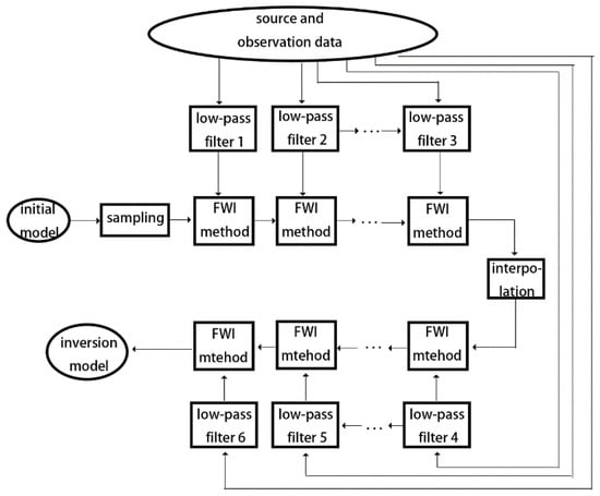
Figure 1.
Schematic diagram of the frequency-grid multiscale method.
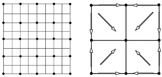
Figure 2.
Schematic diagram of sampling operators (left) and interpolation operators (right).
2.3.2. Envelope Inversion
In theory, nonlinear waveform inversion is difficult because there are many local minimums in the objective function. These local minimums will obstruct the search for the global minimum, and the inversion method will only converge to minimum values that are the nearest to the initial data, as shown in Figure 3.
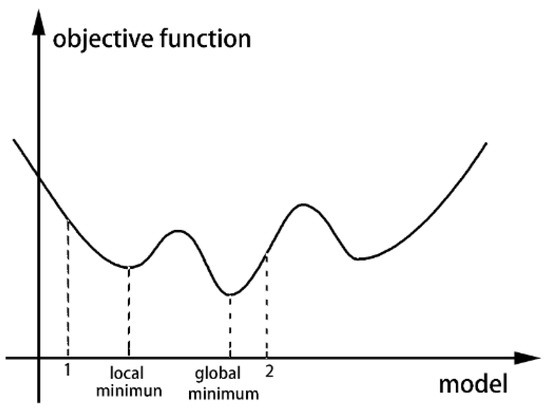
Figure 3.
Schematic diagram of local minimum in the objective function.
When the initial model is close to the actual model, the forward-record data will fall near the global minimum, as in initial value 2; then, inversion iterations can converge to the right solution. When the initial model is further from the actual model, the forward records may fall around the local minimum, as in initial value 1. Then, the inversion iteration results will erroneously converge to the local minimum. This proves that the full-waveform inversion is highly dependent on the initial model, and a good initial model is easier to obtain a better inversion result. Envelope inversion can alleviate this situation. In recent years, many scholars have studied the envelope function and its corresponding properties [35]. By demodulating the low-frequency modulation signal hidden in the observation data with envelope operator, the background field of the medium parameters can be effectively restored and the nonlinear of waveform inversion can be reduced.
The objective function of envelope inversion is as follows:
where and is the envelope of the observed data and the forward simulation data , respectively. , H(u) is the Hilbert transform of seismic records. The gradient derivation of elastic wave envelope inversion is
Equation (17) shows that the inversion based on envelope objective function is identical to the traditional full-waveform inversion except for the back-propagation residuals. Thus, as shown in Figure 4, the envelope inversion was firstly performed and then the results of envelope inversion would be used as the initial model of frequency-grid multiscale method.
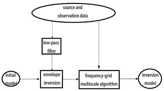
Figure 4.
Schematic diagram of the envelope inversion method.
2.3.3. Joint Velocity–Density Inversion
Forgues and Lambare [36] used ray-approximation and Born-approximation conditions to derive the mathematical expression of the corresponding radiation modes for velocity and density parameterization in a variable-density acoustic wave equation; eigenvalue decomposition analysis of the Hessian matrix was used to show that density inversion is more difficult than velocity inversion. In a 2013 paper, Dong et al. [37] analyzed the relationship between the perturbations of different model parameters and changes in objective function and found that perturbations by long waves in velocity will severely interfere with the density inversion results. One proposed solution is to first carry out large-offset velocity inversion to obtain the medium and long wavelength component in velocity before carrying out simultaneous velocity and density inversion. However, this method cannot avoid the influence of high-frequency components of density on velocity inversion.
Therefore, this study employed another joint inversion method [38,39]: First, the simultaneous inversion of velocity and density was conducted to obtain better velocity parameters and worse density parameters. Then, the velocity obtained in the first step and the initial density were used in the second step as the initial model for velocity and density to conduct another simultaneous inversion. This was able to obtain a better velocity model as well as a better density model.
3. Numerical Experiment
In this chapter, full waveform inversion algorithm is applied to ultrasonic bone density detection. The sound source waveform used is Ricker wavelet:
The source used Ricker wavelets with a central frequency of = 400 kHz. Figure 5 shows the schematic diagram for the waveforms ().
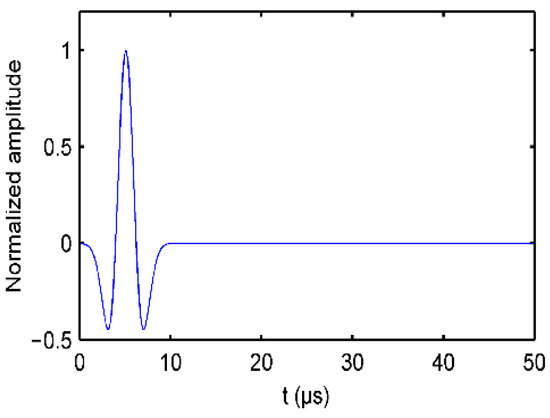
Figure 5.
Full waveforms of Ricker wavelets at the time domain.
3.1. Inversion Results of the Simple Cancellous Bone
When full-waveform inversion was used for bone quantitative measurements, the inversion results were mainly dependent on whether accurate cancellous bone or cortical bone velocity–density parameters could be obtained. Therefore, before conducting complex bone quantitative inversion, we first conducted a detailed assessment of the inversion status of simple cancellous bone or cortical bone. Figure 6 shows the simple cancellous bone model parameters.
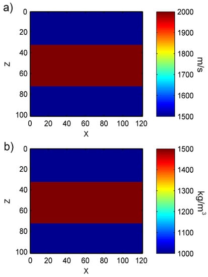
Figure 6.
Cancellous bone model parameters: (a) velocity parameters, (b) density parameters.
As shown in Figure 6, the velocity for the cancellous bone layer is set as 2000 m/s, and density is set as 1500 kg/m3. The velocity for the surrounding soft tissues and couplant is set as 1500 m/s, the density is 1000 kg/m3. Figure 7 shows the inversion results.

Figure 7.
Cancellous bone inversion results based on the improved full-waveform inversion algorithm: (a) velocity model, (b) density model.
From the Figure 7, we can see that our improved full-waveform inversion algorithm can clearly obtain the velocity structure and density structure for cancellous bone. However, the model does not show good effect for velocity and density on the left or right side. This is because there is overlap between the coverage ranges for wavenumber for the diffraction angle of every source–receiver pair. The number of overlapping regions in the center is higher; thus, the inversion results are better. Meanwhile, the number of overlapping regions on the left and right sides is lower; thus, the inversion results are worse. This situation does not pose a significant problem. In actual measurements, the horizontal size of the model can be slightly expanded. In the inversion results thus obtained, the left and right sides that have larger errors can be ignored while only focusing on the bone quantitative parameters in the central region. The next sections will discuss some parameter settings in the inversion method.
3.2. The Influence of Observation System on Inversion Results
The observation system is the array of ultrasonic source point and receiving point. The conventional seismic exploration field can only set up the observation system on the surface, but in the bone density measurement, the setting of the observation system can be more flexible. As shown in Figure 8, ultrasonic source and receiving point arrays can be set on both upper and lower surfaces in bone mineral density measurement. Then we will explore the influence of observation system setting on inversion results.
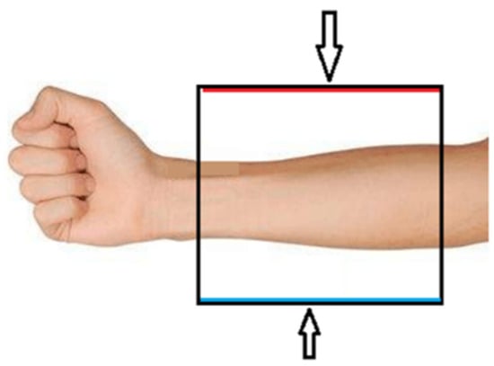
Figure 8.
Settings of the actual observation system.
3.2.1. Distribution of Sources and Receivers
Figure 9 shows a few distribution modes for sources and receivers. In (a), the 20 sources are uniformly distributed on the 0–40 mm on red line at the left of the top of the model, and the spacing is 2 mm. The 60 receivers are uniformly located at the 60–120 mm blue line at the right of the top, and the spacing is 1 mm. In (b), the 20 sources are uniformly distributed on the red line at the top, and the spacing is 6 mm. The 60 receivers are uniformly located on the blue line at the top, and the spacing is 2 mm. The red and blue lines coincide. In (c), the 20 sources are uniformly distributed on the red line at the top and the spacing is 6 mm. The 60 receivers are uniformly located on the blue line at the bottom, and the spacing is 2 mm. In (d), the 20 sources are uniformly distributed on the red line at the top, and the spacing is 6 mm. 30 receivers are uniformly located on the blue line at the top, while the rest 30 receivers are uniformly located on the blue line at the bottom, the spacing is 4 mm.
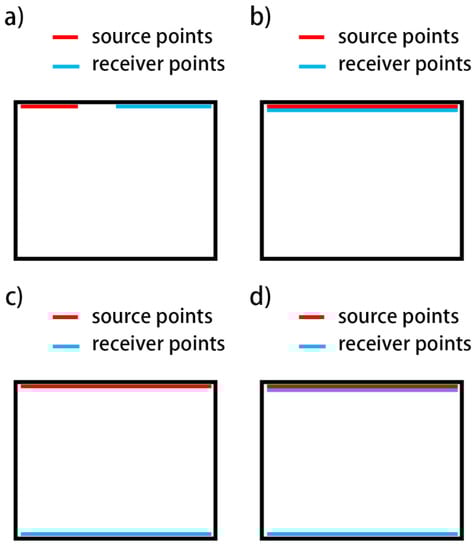
Figure 9.
Different distributions of sources and receivers. (a) the 20 sources are uniformly distributed on the 0–40 mm on red line at the left of the top of the model, and the spacing is 2 mm. The 60 receivers are uniformly located at the 60–120 mm blue line at the right of the top, and the spacing is 1 mm; (b) the 20 sources are uniformly distributed on the red line at the top, and the spacing is 6 mm. The 60 receivers are uniformly located on the blue line at the top, and the spacing is 2 mm. The red and blue lines coincide; (c) the 20 sources are uniformly distributed on the red line at the top and the spacing is 6 mm. The 60 receivers are uniformly located on the blue line at the bottom, and the spacing is 2 mm; (d) the 20 sources are uniformly distributed on the red line at the top, and the spacing is 6 mm. 30 receivers are uniformly located on the blue line at the top, while the rest 30 receivers are uniformly located on the blue line at the bottom, the spacing is 4 mm.
Figure 10 shows the velocity inversion results for four distribution types. In Figure 10a, the velocity distribution of cancellous bone in Figure 7 can hardly be seen, which is a failure of inversion. The main reason for this is insufficient wavenumber coverage range. The inversion image in Figure 10b is a little similar to the objective model while the inversion results at the top half are better than the bottom half. This is because the sources and receivers are mostly located at the top half of the model while the velocity parameters at the bottom half of the inversion results were hardly updated and have a larger overall error. In Figure 10c, the velocity result at the bottom half is getting better because the coverage ability in the vertical direction are strengthened. The inversion results for Figure 10d are the best since they effectively reflect the velocity parameters for the objective model. This shows that the receivers at the bottom half have compensated for the insufficient diffraction angle in the top half. Figure 11 shows the comparison of the velocity inversion results of the four graphs in Figure 10 with the velocity of the objective model. In Figure 11, the x-coordinates represent the number of grid points in the vertical direction while the y-coordinates represent the mean velocity of every row. In this figure, we can see that when the receivers are located at the two sides of the model, the inversion velocity and objective model velocity have the smaller errors, followed by when the sources and receivers are both located on the top surface. Under these conditions, the variation pattern of density is the same as the velocity, which will not be elaborated here. The velocity inversion results were used only as a reference.
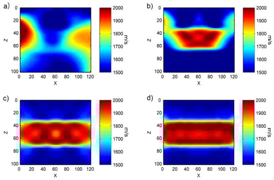
Figure 10.
Velocity inversion results for the four different source-receiver distributions; (a–d) correspond to the source-receiver distribution statuses in Figure 9a–d, respectively.
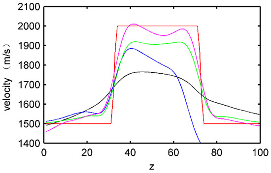
Figure 11.
Comparison of inversion velocity and objective velocity under different source-receiver distributions. In the figure, the red lines represent the velocity of the objective model, and black, blue, green, and magenta lines represent the mean values for each row of inversion velocity under the four source-receiver distributions in Figure 10a–d, respectively.
3.2.2. Quantity of Sources and Receivers
During normal inversion, a suitable quantity of sources and receivers should be selected. If the number is too many, the computational load will increase, and errors will accumulate. If the number is too little, insufficient data will also cause larger errors. Figure 12 shows the velocity inversion results under different numbers of sources and the same number of receivers.
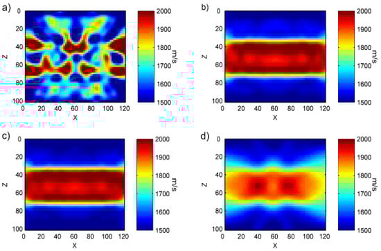
Figure 12.
Velocity inversion results under different numbers of sources. In (a), 60 sources are uniformly distributed at the top of the model, and the spacing is 2 mm; in (b), 30 sources are uniformly distributed at the top of the model, and the spacing is 4 mm; in (c), 20 sources are uniformly distributed at the top of the model, and the spacing is 8 mm; in (d), 10 sources are uniformly distributed at the top of the model, and the spacing is 12 mm.
We can see from the velocity inversion images that an accurate velocity image was almost not obtained in Figure 12a. This is because when there is an excessive number of sources, the wave field values superimposed on every receiver will increase, thereby causing the residual between the forward data and the observed data to be overly large, and accurate least squares solutions cannot be obtained. This results in inversion failure. In Figure 12d, an approximate image of velocity with a large error was obtained. This is because the number of sources is too little, and there is insufficient coverage, causing accurate inversion results to be obtained for some areas while other areas show large differences. Therefore, an accurate selection of the number of sources can not only enable accurate inversion results to be obtained (Figure 12b), but also reduce computational load.
Figure 13 shows the velocity inversion results under different numbers of receivers and the same number of sources. Figure 13a,b show almost consistent inversion results. This indicates that when the number of receivers reaches a certain quantity, the continued addition of receivers will not result in better inversion results but instead will increase computational load. Figure 13c,d is similar to Figure 12c since only a velocity for the approximate model with a larger error was obtained. This is because when the number of receivers is too low, the information used for inversion is too little, and some of forward data are missing. This results in poor inversion results, and the fine updating of model parameters cannot be carried out, causing the output image to have a smooth effect. Figure 14 shows the comparison of the velocity inversion results between Figure 13 and Figure 12. In Figure 14, the x-coordinates represent the number of grid points in the vertical direction while the y-coordinates represent the mean velocity of every row. We can clearly see in Figure 14 that the magenta and blue dotted lines almost coincide, with the green solid and blue solid lines being slightly worse, and the green dotted line being the worst. This is consistent with our abovementioned conclusions.
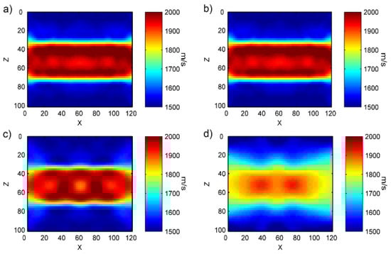
Figure 13.
Velocity inversion results of Figure 12 under different numbers of receivers.
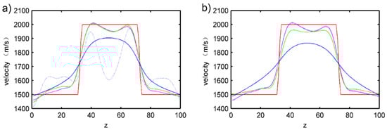
Figure 14.
Comparison of inversion velocity and objective velocity under different source-receiver quantities. In (a), the red lines represent the velocity of the objective model, and blue dotted, green, magenta, and blue solid lines represent the mean values for each row of inversion velocity under the four source distributions in Figure 12a–c, respectively; In (b), the red lines represent the velocity of the objective model, and blue dotted, magenta, green, and blue solid lines represent the mean values for each row of inversion velocity under the four receiver distributions in Figure 13a–d, respectively. Figure 12c and Figure 13b has the same distribution status.
3.2.3. Time Sampling
Appropriate time point sampling during the inversion process can significantly reduce computational load without reducing inversion quality. The example in Figure 15 shows the velocity inversion images under different time sampling rates. We can see from the figure that an appropriate increase in the sampling time interval will not affect the inversion results: there are not many differences in the results between data sampling at every eight time steps, every four time steps, and every two time steps. Figure 16 shows the error between inversion velocity and the objective model under different sampling rates. The x-coordinates represent the number of grid points in the vertical direction while the y-coordinates represent the mean velocity of every row. It can be seen that the three velocity curves are close to the velocity curve of the objective model.
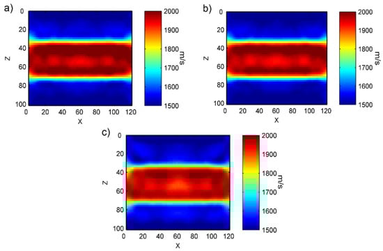
Figure 15.
Velocity inversion results under different time sampling rates in forward simulation data. (a) Data are extracted every 2 time steps for participation in the inversion algorithm. (b) Data are extracted every 4 time steps for participation in the inversion algorithm. (c) Data are extracted every 8 time steps for participation in the inversion algorithm.
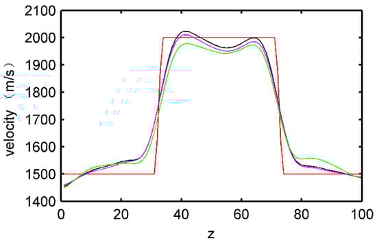
Figure 16.
Comparison of inversion velocity and objective velocity under different time sampling rates. In the figure, the red lines represent the velocity of the objective model, and black, magenta, and green lines represent the mean values for each row of inversion velocity under the three different time sampling rates in Figure 15a–c, respectively.
3.2.4. Resolution Ability of Parameter Variation
An advantage of the full-waveform inversion algorithm is that it can be used to obtain the geometric distribution of bone model structural parameters and not just the mean density. During the early stage of osteoporosis, only some density changes occur in bone tissues, and the density is extremely close to that of the surrounding normal bone tissues. It is easy to overlook these changes if only an averaging method is used to obtain BMD or if the resolution of the measurement algorithm is not high. Therefore, the ability to differentiate minor parameter changes in bone tissues is also a judgment criterion for whether the method used for bone quantitative measurement is good. We designed a model, as shown in Figure 16, to validate the resolution of the modified full-waveform algorithm in small-parameter variations.
In Figure 17, cancellous bone is divided into two parts, with the upper half having a velocity of 1950 m/s, and a density of 1450 kg/m3, and the bottom half having a velocity of 2000 m/s, and a density of 1500 kg/m3. The difference between the two velocities is 50 m/s and the difference between the two densities is 50 kg/m3.
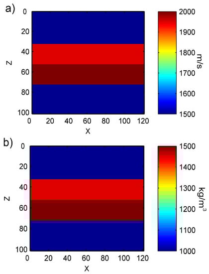
Figure 17.
Objective model parameters for small-parameter variations in cancellous bone: (a) velocity parameters, (b) density parameters.
In Figure 18, we can see that the inversion results for the velocity model are relatively good as the velocity difference between the two layers could be clearly reflected. The density inversion results are slightly worse. It can still invert the different densities of the two layers, but the dividing line is not flat. This experiment demonstrates the resolution capabilities of full-waveform inversion on small-parameter variations. Figure 19 shows the comparison chart for velocity and density between the inversion results and the objective model. The x-coordinates represent the number of grid points in the vertical direction while the y-coordinates represent the mean velocity of every row.
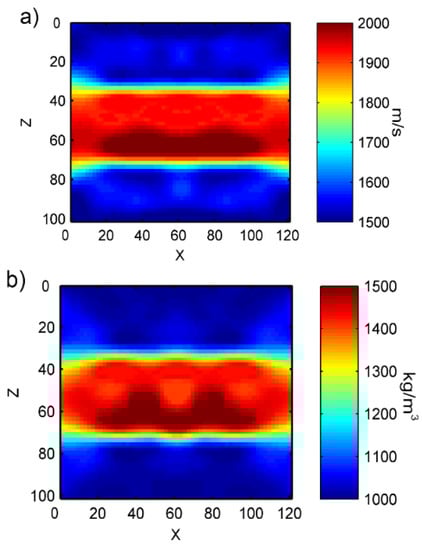
Figure 18.
Inversion results for small-parameter variations in cancellous bone: (a) velocity model; (b) density model.
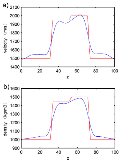
Figure 19.
Comparison of inversion velocity and objective velocity for small-parameter variations in cancellous bone. The red lines represent the parameters of the objective model, and the blue lines represent inversion parameters. (a) Velocity parameters, (b) density parameters.
3.3. The Inversion Results of Simple Cortical Bone Model
With regard to cortical bone models, since the model parameter differences between bones and the surrounding soft tissues are relatively large, the objective function tends to easily fall into local minimum during inversion. The use of a frequency-grid multiscale algorithm can effectively prevent the generation of local minimum. Figure 20 shows the simple cortical bone model parameters.
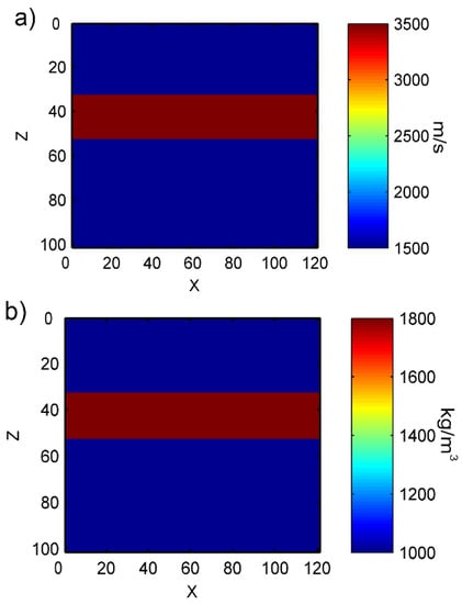
Figure 20.
Cortical bone model parameters: (a) velocity parameters, (b) density parameters.
As shown in Figure 20, the velocity for the cortical bone layer is set as 3500 m/s, and density is set as 1800 kg/m3. The velocity for the surrounding soft tissues and couplant is set as 1500 m/s, and the density is 1000 kg/m3. We can see in Figure 21 that accurate inversion results were obtained using the frequency-grid multiscale algorithm.
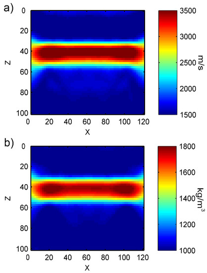
Figure 21.
Cortical bone inversion results based on the improved full-waveform inversion algorithm: (a) velocity model, (b) density model.
3.4. The Long Bone Inversion
3.4.1. Gridding of Long Bone Model Parameters
In the above two large experiments, we discussed the inversion methods and results for cancellous bone and cortical bone. If good inversion results could be obtained for both cancellous bone and cortical bone, it would demonstrate that the improved full-waveform inversion algorithm proposed in this study can be used in bone quantitative measurements for complex bone structures. Below, we describe the numerical experiment in which inversion was used for long bones.
In Figure 22, we can see that long bones are mainly composed of cortical bone, cancellous bone, medullary cavity, epiphysis, and periosteum. Based on differences in the velocities of ultrasonic waves in different parts of long bones, we can obtain the geometric distribution of long bone velocity and density parameters using FWI, thereby obtaining the internal structure of long bones and calculating their BMD. We divided the long bone into two segments and designed the objective model as shown in Figure 23.
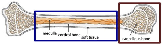
Figure 22.
A long bone structure.
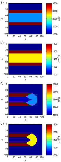
Figure 23.
Gridding of long bone model approximation parameters; (a,b) are the velocity parameters and density parameters, respectively, in the middle segments of long bone; (c,d) are the velocity parameters and density parameters, respectively, in the end segments of long bone.
In the middle segment of long bone, the deep-red color represents the velocity and density of cortical bone media, set at 3500 m/s and 1800 kg/m3 respectively. Light-blue represents the velocity parameters for bone marrow, and yellow represents the density. Bone marrow usually fills the gap between the medullary cavity and cancellous bone. In this study, the velocity and density parameters are assumed to be 2000 m/s and 1500 kg/m3, respectively. The blue at the top and bottom of the deep-red regions represents the surrounding soft tissues of the bone, and the velocity is set at 1500 m/s, and the density is 1000 kg/m3. In the ends of long bone, the deep-red color also represents cortical bone media, with a velocity of 3500 m/s and a density of 1800 kg/m3. The light-blue on the right represents cancellous bone, with a velocity of 2000 m/s and a density of 1500 kg/m3. The deep-red middle represents the bone marrow. As the bone marrow content in the medullary cavities at the ends of long bone is relatively less, the velocity is set at 1600 m/s and the density is 1000 kg/m3. The top and bottom sides of the deep-red similarly represent soft tissues with a velocity of 1500 m/s and a density of 1000 kg/m3.
3.4.2. Results of Long Bone Middle Segment Inversion
In Figure 24a,b, we can clearly see the distribution status of velocity parameters and density parameters, with clear boundaries. To better compare the differences between the inversion results and the objective model, Equations (19) and (20) were used to calculate the row mean relative error and column mean relative error between the inversion model parameters and the objective model parameters. In the equation, and represent the number of grid points in a row and a column, respectively. represents the model parameter value of the inversion result at the x row and z column. represents the objective model parameter value at the x row and z column. Figure 25 shows the curves for and . In this figure, we can see that the error for the density inversion results is slightly lower than for the velocity inversion results. This is because, in the long bone model, the density changes between bones and soft tissue are gentler than the velocity changes. With regard to row mean relative error, places with drastic parameter changes have larger errors. The maximum value for velocity error is 0.07, while the maximum value for density error is 0.06, and the minimum values are both close to 0. With regard to column mean relative error, the errors at the left and right ends are relatively larger while the central region is more uniform. The maximum value for velocity error is around 0.035 and the minimum value is around 0.017, while the maximum value for density error is around 0.025 and the minimum value is around 0.01. Equation (21) was used to calculate the mean relative error of the entire inversion result as . The mean relative error for the obtained velocity is 0.0257, and density is 0.0163. This means the error between the inversion velocity and the actual velocity is only around 2%, which conforms to the standards for actual applications.
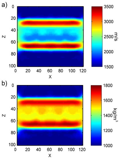
Figure 24.
Inversion results of the long bone middle segment: (a) velocity model; (b) density model.
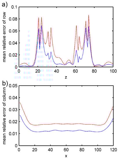
Figure 25.
Mean relative error between the inversion model and objective model of the long bone middle segment. Red shows the error between velocity parameters and blue shows the error between density parameters (a) mean relative error of row; (b) mean relative error of column.
3.4.3. Results of Long Bone End Segment Inversion
Similar to the long bone middle segment inversion results in the previous section, Figure 26a,b clearly show the distribution of velocity and density parameters, whose boundaries are clear. We can see in this figure that the overall trend is similar to the inversion of the long bone middle segment. In Figure 27, with regard to row mean relative error, places with drastic parameter changes have larger errors. The maximum value for velocity error is 0.07, the minimum is close to 0; while for density error, the maximum is 0.06, and the minimum is close to 0. With regard to column mean relative error, the errors at the left are relatively larger while the central region is more uniform, and the right end is the smallest. The maximum value for velocity error is around 0.04 and the minimum is around 0; so are for the density error. The mean relative error for the obtained velocity is 0.0198, and density is 0.0185. This means the errors between inversion velocity and actual velocity as well as inversion density and actual density are both less than 2%, which also conforms to the standards of actual application.
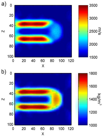
Figure 26.
Inversion results of the long bone end segment: (a) velocity model; (b) density model.
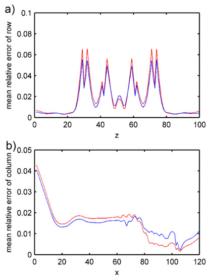
Figure 27.
Mean relative error between the inversion model and objective model of the long bone end segment. Red shows the error between velocity parameters and blue shows the error between density parameters (a) mean relative error of row; (b) mean relative error of column.
3.4.4. Noise
To simulate electromagnetic noise during measurement or other small interference noise in the environment, we added suitable amounts of observation noise to the observation data. The specific steps were as follows: Gaussian noise with a standard deviation of 10% was added to the wave field records obtained from the forward simulation of the objective model. The noise generation method is shown in [40]. The wave field record containing noise interference was taken as observation data for inversion. As shown in Figure 28, we selected three receivers (the second and thirteenth points from the left on the top surface, and the seventh point from the left of the bottom surface) to observe the forward records of the objective model after adding noise.
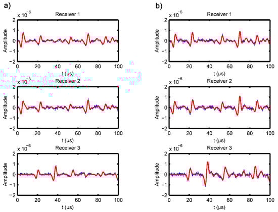
Figure 28.
Forward records of different receivers, red line is the record with no noise, while blue line is the record with 10% Gauss noise: (a) middle segment model of long bone; (b) end segment model of long bone.
We can see in Figure 29 that after the addition of 5% Gaussian noise, there was not much difference in the inversion results compared to the inversion results without added noise, with only some nonuniform regions in background velocity caused by noise interference. This is mainly because the smoothing function introduced in this paper was used to regularize the objective function, which decreases the effects of noise in the observation data. The inversion results in Figure 29 demonstrate the robustness of our improved full-waveform inversion algorithm for bone quantitative measurement.
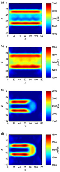
Figure 29.
Inversion results of long bone model parameters containing noise: (a) velocity inversion results for middle segment of long bone; (b) density inversion results for middle segment of long bone; (c) velocity inversion results for end segment of long bone; (d) density inversion results for end segment of long bone.
3.5. Inversion Results of the Tibia and Fibula Model
The tibia is an important bone in the calf that supports the weight of the body while the fibula is attached to the calf muscles and bears one-sixth of body weight. The two bones are connected as one by the superior tibia–fibula joint and the inferior tibia–fibula joint, and they are important bones in human BMD measurements. As shown in Figure 30, we selected a segment in the middle of the tibia–fibula pair as an objective model to better validate the extensiveness of our modified FWI algorithm. The approximate objective model is as follows:
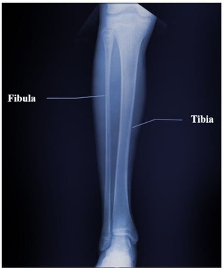
Figure 30.
Structure of the tibia–fibula bone pair.
As in Figure 31, the deep-red color represents the velocity and density of bone tissues, set at 3500 m/s and 1800 kg/m3, respectively. The blue regions represents the surrounding soft tissues of the bone, and the velocity is set at 1500 m/s, and the density is 1000 kg/m3. We present the inversion results in Figure 32. Like the previous results, our method can clearly get the good distribution of the velocity and density parameters of tibia–fibula bone pair model. There are some bad results on the left and right side of the image, because there are more cortical bone structures in the objective model, thus increasing the contrast with the surrounding soft tissue parameters and affecting the inversion results. As before, we can also expand the range of the measurement part in the actual situation and intercept the middle part of the inversion image. Figure 33 shows the row mean relative error and column mean relative error between the inversion model parameters and the objective model parameters. With regard to row mean relative error, the maximum value for velocity error is 0.08, the minimum is close to 0; while for density error, the maximum is 0.04, and the minimum is close to 0. With regard to column mean relative error, the maximum value for velocity error is around 0.04 and the minimum is around 0.03; while the maximum value for density error is around 0.04 and the minimum value is around 0.01. The mean relative error for the obtained velocity is 0.0386, and density is 0.0207.
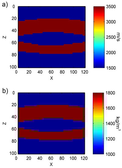
Figure 31.
Gridding of a tibia–fibula bone pair model approximation parameters: (a) velocity parameters; (b) density parameters.
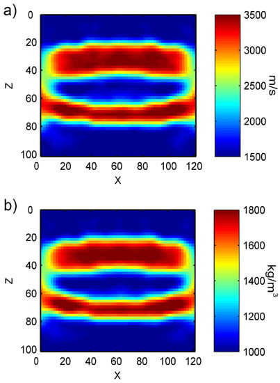
Figure 32.
Inversion results of tibia–fibula bone pair model: (a) velocity model; (b) density model.
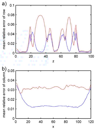
Figure 33.
Mean relative error between the inversion model and objective model of tibia–fibula bone pair model. Red shows the error between velocity parameters and blue shows the error between density parameters (a) mean relative error of row; (b) mean relative error of column.
We also add 10% Gauss noise to the observed record to imitate the additional interference in the measurement as shown in Figure 34. We selected three receivers (the second and thirteenth points from the left on the top surface, and the seventh point from the left of the bottom surface) to observe the forward records of the objective model after adding noise as well. As can be seen from Figure 35, the added noise has little effect on the inversion result.
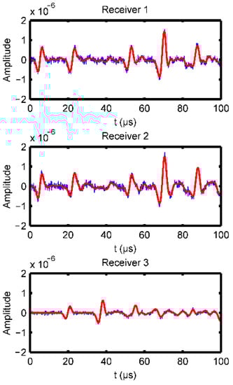
Figure 34.
Forward records of different receivers, red line is the record with no noise, while blue line is the record with 10% Gauss noise.
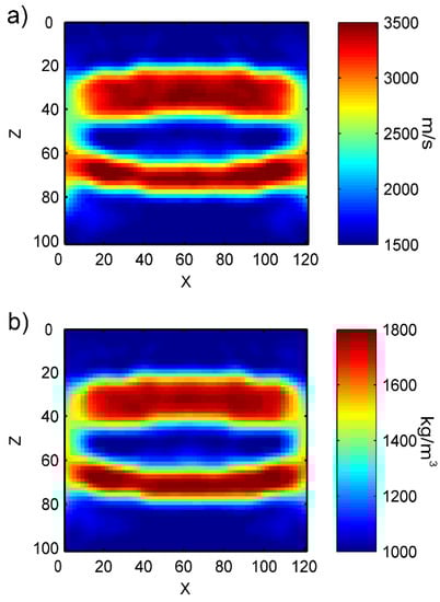
Figure 35.
Inversion results of tibia–fibula bone pair model parameters containing noise: (a) velocity inversion results; (b) density inversion results.
4. Discussion
The numerical experiments showed that the proposed method in this study could successfully obtain the value and distribution of the velocity parameters and density parameters of the designed model. In the inversion section, the authors examined and adopted numerical experiments to verify the effects of the distribution and quantity of source-receivers, time sampling rate, and parameter resolution on the inversion results. The experiments showed that when the measurement image is a two-dimensional section along the long axis of the bone, the broader the distance range between the sources and receivers, the better the results. In addition, the receivers should be located on both sides, with some located on the same side of the sources and some located on the opposite side of the sources. At the same time, an appropriate number of sources and receivers should be selected. When the number of source or receivers is too many, “over-sampling” may sometimes lead to inversion failure or increased computational load. When the number of source or receivers is too few, insufficient sampling may lead to overly large errors in the inversion results. The experiments also showed that an appropriate time sampling rate can greatly reduce computational load without affecting the inversion results. When the measurement part contains more cortical bone, and the differences between the initial model and objective model parameters are too great, the use of a frequency-grid multiscale algorithm can improve the inversion results.
In summary, the improved FWI method proposed in this paper shows superior inversion results as it can detect small velocity–density changes in bones, and the relative error of the numerical model is within 2%. This method can also avoid interference from small amounts of noise and satisfy the high precision requirements for quantitative ultrasound measurements of bone.
5. Conclusions
This study improved the FWI algorithm which is usually used in conventional seismic image processing and successfully applied it to quantitative ultrasound measurement for bones. Numerical experiments demonstrated that our modified full-waveform inversion algorithm is effective and robust for clinical bone quantitative measurement. However, bones should be considered as anisotropic media in actual measurement rather than isotropic elastic hypothesis. This requires more computational load, and will be a challenge for our future work in actual bone quantitative measurements.
Author Contributions
Conceptualization, Methodology, Writing—original Draft Preparation, and Writing—review and editing, M.S.; Validation and Supervision D.Z. and Y.Y. All authors have read and agreed to the published version of the manuscript.
Funding
We are grateful for the financial support from the Major National Science and Technology Project of China (Grant number: 2011ZX05003-003).
Institutional Review Board Statement
Not applicable.
Informed Consent Statement
Not applicable.
Data Availability Statement
Publicly available datasets were analyzed in this study. This data can be found here: https://doi.org/10.3390/sym13020260.
Conflicts of Interest
The authors declare no conflict of interest.
References
- Rayalam, S.; Della-Fera, M.A.; Baile, C.A. Synergism between resveratrol and other phytochemicals: Implications for obesity and osteoporosis. Mol. Nutr. Food Res. 2011, 55, 1177–1185. [Google Scholar] [CrossRef]
- Chin, K.-Y.; Ima-Nirwana, S. Can Soy Prevent Male Osteoporosis? A Review of the Current Evidence. Curr. Drug Targets 2013, 14, 1632–1641. [Google Scholar] [CrossRef]
- Schuit, S.C.E.; van der Klift, M.; Weel, A.; de Laet, C.; Burger, H.; Seeman, E.; Hofman, A.; Uitterlinden, A.G.; van Leeuwen, J.; Pols, H.A.P. Fracture incidence and association with bone mineral density in elderly men and women: The Rotterdam Study. Bone 2004, 34, 195–202. [Google Scholar] [CrossRef]
- Kalender, W.A.; Felsenberg, D.; Genant, H.K.; Fischer, M.; Dequeker, J.; Reeve, J. The European spine phantom—A tool for standardization and quality-control in spinal bone-mineral measurements by DXA and QCT. Eur. J. Radiol. 1995, 20, 83–92. [Google Scholar] [CrossRef]
- Guglielmi, G.; Damilakis, J.; Solomou, G.; Bazzocchi, A. Quality assurance of imaging techniques used in the clinical management of osteoporosis. Radiol. Med. 2012, 117, 1347–1354. [Google Scholar] [CrossRef]
- Ruegsegger, P.; Koller, B.; Muller, R. A microtomographic system for the nondestructive evaluation of bone architecture. Calcif. Tissue Int. 1996, 58, 24–29. [Google Scholar] [CrossRef] [PubMed]
- Schneider, R. Imaging of Osteoporosis. Rheum. Dis. Clin. N. Am. 2013, 39, 609. [Google Scholar] [CrossRef]
- Laugier, P.; Droin, P.; LavalJeantet, A.M.; Berger, G. In vitro assessment of the relationship between acoustic properties and bone mass density of the calcaneus by comparison of ultrasound parametric imaging and quantitative computed tomography. Bone 1997, 20, 157–165. [Google Scholar] [CrossRef]
- Edelmann-Schaefer, B.; Berthold, L.D.; Stracke, H.; Luehrmann, P.M.; Neuhaeuser-Berthold, M. Identifying elderly women with osteoporosis by spinal dual X-Ray absorptiometry, calcaneal quantitative ultrasound and spinal quantitative computed tomography: A comparative study. Ultrasound Med. Biol. 2011, 37, 29–36. [Google Scholar] [CrossRef] [PubMed]
- Langton, C.; Palmer, S.; Porter, R. The Measurement of Broadband Ultrasonic Attenuation in Cancellous Bone. Eng. Med. 1984, 13, 89–91. [Google Scholar] [CrossRef] [PubMed]
- Raum, K.; Grimal, Q.; Varga, P.; Barkmann, R.; Glueer, C.C.; Laugier, P. Ultrasound to Assess Bone Quality. Curr. Osteoporos. Rep. 2014, 12, 154–162. [Google Scholar] [CrossRef]
- Glüer, C.; Yang, L.; Reid, D.; Felsenberg, D.; Roux, C.; Barkmann, R.; Timm, W.; Blenk, T.; Armbrecht, G.; Stewart, A.; et al. Association of Five Quantitative Ultrasound Devices and Bone Densitometry with Osteoporotic Vertebral Fractures in a Population-Based Sample: The OPUS Study. J. Bone Miner. Res. Off. J. Am. Soc. Bone Miner. Res. 2004, 19, 782–793. [Google Scholar] [CrossRef]
- Krieg, M.-A.; Cornuz, J.; Ruffieux, C.; Melle, G.; Bueche, D.; Dambacher, M.; Hans, D.; Hartl, F.; Häuselmann, H.; Kraenzlin, M.; et al. Prediction of Hip Fracture Risk by Quantitative Ultrasound in More than 7000 Swiss Women ≥ 70 Years of Age: Comparison of Three Technologically Different Bone Ultrasound Devices in the SEMOF Study. J. Bone Miner. Res. Off. J. Am. Soc. Bone Miner. Res. 2006, 21, 1457–1463. [Google Scholar] [CrossRef]
- Marin, F.; Gonzalez-Macias, J.; Diez-Perez, A.; Palma, S.; Delgado-Rodriguez, M. Relationship Between Bone Quantitative Ultrasound and Fractures: A Meta-Analysis. J. Bone Miner. Res. Off. J. Am. Soc. Bone Miner. Res. 2006, 21, 1126–1135. [Google Scholar] [CrossRef] [PubMed]
- Tarantola, A. Inversion of seismic data in acoustic approximation. Geophysics 1984, 49, 1259–1266. [Google Scholar] [CrossRef]
- van Dongen, K.W.A.; Wright, W. A forward model and conjugate gradient inversion technique for low-frequency ultrasonic imaging. J. Acoust. Soc. Am. 2006, 120, 2086–2095. [Google Scholar] [CrossRef] [PubMed]
- Li, C.; Duric, N.; Littrup, P.; Huang, L. In vivo Breast Sound-Speed Imaging with Ultrasound Tomography. Ultrasound Med. Biol. 2009, 35, 1615–1628. [Google Scholar] [CrossRef]
- Bernard, S.; Monteiller, V.; Komatitsch, D.; Lasaygues, P. Ultrasonic computed tomography based on full-waveform inversion for bone quantitative imaging. Phys. Med. Biol. 2017, 62, 7011–7035. [Google Scholar] [CrossRef]
- Marfurt, K.J. Accuracy of finite-difference and finite-element modeling of the scalar and elastic wave-equations. Geophysics 1984, 49, 533–549. [Google Scholar] [CrossRef]
- Kreiss, H.-O.; Oliger, J. Comparison of accurate methods for the integration of hyperbolic equations. Tellus 1972, 24, 199. [Google Scholar] [CrossRef]
- Virieux, J. P-SV wave propagation in heterogeneous media; velocity-stress finite-difference method. Geophysics 1986, 51, 889–901. [Google Scholar] [CrossRef]
- Kelly, K.R.; Ward, R.W.; Treitel, S.; Alford, R.M. Synthetic seismograms: A finite-difference approach. Geophysics 1976, 41, 2–27. [Google Scholar] [CrossRef]
- Moczo, P.; Kristek, J.; Gális, M. The Finite-Difference Modelling of Earthquake Motions: Waves and Ruptures; Cambridge University Press: Cambridge, UK, 2014. [Google Scholar]
- Moczo, P.; Kristek, J.; Galis, M.; Chaljub, E.; Etienne, V. 3-D finite-difference, finite-element, discontinuous-Galerkin and spectral-element schemes analysed for their accuracy with respect to P-wave to S-wave speed ratio. Geophys. J. Int. 2011, 187, 1645–1667. [Google Scholar] [CrossRef]
- Sourbier, F.; Operto, S.; Virieux, J.; Amestoy, P.; L’Excellent, J.-Y. FWT2D: A massively parallel program for frequency-domain full-waveform tomography of wide-aperture seismic data-Part 2 Numerical examples and scalability analysis. Comput. Geosci. 2009, 35, 496–514. [Google Scholar] [CrossRef]
- Crase, E.; Pica, A.; Noble, M.; McDonald, J.; Tarantola, A. Robust elastic nonlinear wave-form inversion-application to real data. Geophysics 1990, 55, 527–538. [Google Scholar] [CrossRef]
- Pratt, R.G.; Shin, C.; Hicks, G.J. Gauss-Newton and full Newton methods in frequency-space seismic waveform inversion. Geophys. J. Int. 1998, 133, 341–362. [Google Scholar] [CrossRef]
- Shin, G.; Jang, S.; Min, D.J. Improved amplitude preservation for prestack depth migration by inverse scattering theory. Geophys. Prospect. 2001, 49, 592–606. [Google Scholar] [CrossRef]
- Nocedal, J. Updating quasi-newton matrices with limited storage. Math. Comput. 1980, 35, 773–782. [Google Scholar] [CrossRef]
- Köhn, D. Time Domain 2D Elastic Full Waveform Tomography. Ph.D. Thesis, Christian-Albrechts-Universität zu Kiel, Kiel, Germany, July 2011. [Google Scholar]
- Wang, S.-D.; Huang, W.-H. A method of velocity inversionof two dimensional acousticwave equation. Chin. J. Geophys. 1995, 38, 833–839. [Google Scholar]
- Beydoun, W.B.; Tarantola, A. 1st born and rytov approximations-modeling and inversion conditions in a canonical example. J. Acoust. Soc. Am. 1988, 83, 1045–1055. [Google Scholar] [CrossRef]
- Pratt, R.; Sirgue, L.; Hornby, B.; Wolfe, J. Crosswell Waveform Tomography in Fine-Layered Sediments-Meeting the Challenges of Anisotropy. In Proceedings of the 70th EAGE Conference and Exhibition incorporating SPE EUROPEC 2008, Rome, Italy, 9–12 June 2008. cp-40-00141. [Google Scholar]
- Bunks, C.; Saleck, F.M.; Zaleski, S.; Chavent, G. Multiscale seismic wave-form inversion. Geophysics 1995, 60, 1457–1473. [Google Scholar] [CrossRef]
- Chi, B.; Dong, L.; Liu, Y. Full waveform inversion method using envelope objective function without low frequency data. J. Appl. Geophys. 2014, 109, 36–46. [Google Scholar] [CrossRef]
- Forgoes, E.; Lambaré, G. Parameterization study for acoustic and elastic ray+born inversion. J. Seism. Explor. 1997, 6, 253–277. [Google Scholar]
- Dong, L.; Ben-Xin, C.H.I.; Ji-Xia, T.A.O.; Liu, Y. Objective-Function Behavior in Acoustic Full-Waveform Inversion. Chin. J. Geophys. 2013, 56, 685–703. [Google Scholar]
- Yang, J.-Z.; Liu, Y.-Z.; Dong, L.-G. A multi-parameter full waveform inversion strategy for acoustic media with variable density. Chin. J. Geophys. Chin. Ed. 2014, 57, 628–643. [Google Scholar]
- Günerhan, H.; Çelik, E. Analytical and approximate solutions of Fractional Partial Differential-Algebraic Equations. Appl. Math. Nonlinear Sci. 2020, 5, 109–120. [Google Scholar] [CrossRef]
- Shin, C.; Min, D.-J. Waveform inversion using a logarithmic wavefield. Geophysics 2006, 71, R31–R42. [Google Scholar] [CrossRef]
Publisher’s Note: MDPI stays neutral with regard to jurisdictional claims in published maps and institutional affiliations. |
© 2021 by the authors. Licensee MDPI, Basel, Switzerland. This article is an open access article distributed under the terms and conditions of the Creative Commons Attribution (CC BY) license (http://creativecommons.org/licenses/by/4.0/).