Fourier Spectral High-Order Time-Stepping Method for Numerical Simulation of the Multi-Dimensional Allen–Cahn Equations

Abstract

This paper introduces the Fourier spectral method combined with the strongly stable exponential time difference method as an attractive and easy-to-implement alternative for the integration of the multi-dimensional Allen–Cahn equation with no-flux boundary conditions. The main advantages of the proposed method are that it utilizes the discrete fast Fourier transform, which ensures efficiency, allows an extension to two and three spatial dimensions in a similar fashion as one-dimensional problems, and deals with various boundary conditions. Several numerical experiments are carried out on multi-dimensional Allen–Cahn equations including a two-dimensional Allen–Cahn equation with a radially symmetric circular interface initial condition to demonstrate the fourth-order temporal accuracy and stability of the method. The numerical results show that the proposed method is fourth-order accurate in the time direction and is able to satisfy the discrete energy law.

1. Introduction

In this paper, we consider the following nonlinear Allen–Cahn (AC) equation with the homogeneous Neumann boundary condition:

$$\begin{array}{ccc}\hfill & \frac{\partial u(x,t)}{\partial t}=\Delta u(x,t)-\frac{1}{{ϵ}^2}f\left(u(x,t)\right),(x,t)\in \mathsf{\Omega }\times (0,T]\hfill & \hfill \\ \hfill & u(x,0)=u_0\left(x\right),x\in \mathsf{\Omega }\subset {\mathbb{R}}^d,d=1,2,3.\hfill & \hfill \\ \hfill & \nabla u·\mathbf{n}=0\mathrm{on}\partial \mathsf{\Omega },\hfill & \hfill \end{array}$$

(1)

In the above equation, u represents the concentration of one of the two metallic components of the alloy, $\mathbf{n}$ is the unit normal vector to $\partial \mathsf{\Omega }$, and the parameter $ϵ>0$ represents the interfacial width, which is small with respect to the characteristic length of the laboratory scale. The no-flux boundary condition implies that no mass loss occurs across the boundary of the bounded domain $\mathsf{\Omega }.$$f\left(u\right)$ is a reaction term with $f\left(u\right)=F^{\prime }\left(u\right),$ where $F\left(u\right)$ is a double-well potential.

We assume that the reaction term f is an odd, locally Lipschitz function. In particular, we let $f\left(u\right)=-u(1-u^2),$ so that $F\left(u\right)=\frac{1}{4}{(u^2-1)}^2.$

The Lyapunov energy functional $E\left(u\right)$ corresponding to the AC equation is given by:

$$\begin{array}{cc}\hfill & E\left(u\right)={\int }_{\mathsf{\Omega }}\left(\frac{1}{2}{|\nabla u|}^2+\frac{1}{{ϵ}^2}F(u)\right)dx\hfill \end{array}$$

(2)

which yields the following energy decay property of the system:

$$\begin{array}{cc}\hfill & E^{{}^{\prime }}\left(t\right)\le 0,t\ge 0\hfill \end{array}$$

(3)

and the decreasing property of the energy function guarantees the existence of solutions for the AC equation for the reaction term defined as above [1,2,3].

The AC equation was originally introduced by John W. Cahn and Sam M. Allen in 1979 [4] to describe the phase separation in multicomponent alloy systems, for example, iron-aluminum (Fe-Al) alloy. Allen and Cahn studied the anti-phase boundaries in binary alloys to discover topical changes by creating a phase-field model. These equations are a special type of nonlinear partial differential equations and used initially to solve the phase transition problems, such as transforming a thermodynamic system from one phase to another. The AC equation has also been widely used in many complicated moving interface problems in material science and fluid dynamics, such as the motion by mean curvature flows, image analysis, crystal growth, vesicle membrane fluidity, the nucleation of solids, and the mixture of two incompressible fluids [4,5,6,7,8,9,10,11,12]. In order to develop an understanding related to the nonlinear phenomenon associated with the AC equation, either the exact or numerical solution is required. Since the exact solution of the AC equation is rarely possible due to its nonlinearity, numerical methods play an essential and important role in solving the equation. Therefore, the development of an efficient and accurate numerical method has practical significance and has drawn the attention of many researchers.

The AC equation has been numerically extensively studied in [13,14,15,16,17,18,19,20,21]. For example, Choi et al. [13] developed an unconditionally gradient stable scheme, which is second-order accurate in space and first-order accurate in time to solve the AC equation. T. Tang et al. in [18,19] studied the maximum principle preserving schemes for the generalized AC equation. In [18], the authors used a semi-implicit scheme, whereas in [19], they used an implicit-explicit scheme to discretize the time variable.

The authors in [14,15,16,20] proposed the operator splitting schemesfor the AC equation. H. G. Lee et al. in [15] proposed a simple and stable second-order operator splitting method by decomposing the original equation into three subequations with the free-energy evolution term, the heat evolution term, and a nonlinear source term. Yibao Li et al. in [16] proposed an unconditionally stable second-order hybrid numerical method for solving the AC equation by decomposing the original equation into linear and nonlinear equations. They used a Crank–Nicolson scheme to discretize the linear equation and used a fast solver to solve the resulting discrete system of equations. They then solved the nonlinear equation analytically. Zhang and Du in [21] studied the performance of numerical approximations to the AC-type diffuse interface models, with a particular focus on their performance in the sharp interface limit and the effectiveness of high-order discretization schemes. They first compared the different spatial discretizations of an energy functional in the diffuse interface framework and analyzed discretizations of the time-dependent equation using various time-stepping schemes and an adaptive finite element spatial approximation. In [22,23,24], the authors studied various nonlinear equations for numerical solutions using iterative methods. Gottlieb and Wang in [25] analyzed the stability and convergence of the Fourier pseudospectral method coupled with a variety of specially designed time-stepping methods of up to fourth-order, for the numerical solution of a three-dimensional viscous Burgers’ equation. The long-time stability properties of a few multi-step time discretization schemes with the Fourier pseudospectral method for the two-dimensional incompressible Navier–Stokes equations were studied in [26]. In [27], Chen et al. discussed the long-time energy stability and error analysis of higher order linear exponential time differential (ETD) multi-step methods for gradient flows based on the energy method. A second-order energy stable BDFnumerical scheme was proposed in [28] to solve the Cahn–Hilliard equation.

In this paper, our main aim is to propose a high-order numerical method that can solve the AC equation with a relatively larger time step by explicitly treating the nonlinear term. We propose a Fourier spectral method combined with a strongly stable exponential time difference method as an attractive and easy-to-implement alternative for integrating multi-dimensional AC equations with no-flux boundary conditions. The main benefits of the proposed method are that it utilizes the discrete fast Fourier transform, which ensures efficiency, allows an extension to two and three spatial dimensions in a similar fashion as in the one-dimensional problem, and deals with various boundary conditions. In addition, the proposed method is able to capture the motion of a circle solution of the AC equation with a radially symmetric circular interface initial condition and also satisfies the discrete energy law.

The remainder of the paper is organized as follows. In Section 2, the Fourier spectral method is briefly reviewed. The proposed time-stepping method, with its implementation for 3D AC problems, is explained in Section 3. In Section 4, numerical experiments are performed to test the accuracy and applicability of the proposed method. The conclusions are presented in Section 5, which briefly summarizes the computational results.

2. Fourier Spatial Discretization

In order to utilize the Fourier spectral method on Equation (1) with $x\in \mathsf{\Omega }={(a,b)}^d,d=1,2,3$, we followed the procedure introduced in [29] for a homogenous Neumann boundary condition. Let ${\varphi }_i,{\varphi }_{i,j},\mathrm{or}{\varphi }_{i,j,l}$ be the complete set of orthonormal eigenfunctions corresponding to eigenvalues ${\lambda }_i,{\lambda }_{i,j},\mathrm{or}{\lambda }_{i,j,l}$ of the Laplacian operator $(-\Delta )$ on a bounded region $\mathsf{\Omega }\subset {\mathbb{R}}^d$ with the homogeneous Neumann boundary condition, i.e.,

$$\begin{array}{ccc}\hfill & (-\Delta ){\varphi }_i={\lambda }_i{\varphi }_i,\mathrm{if}d=1\hfill & \\ \hfill & (-\Delta ){\varphi }_{i,j}={\lambda }_{i,j}{\varphi }_{i,j},\mathrm{if}d=2\hfill & \\ \hfill & (-\Delta ){\varphi }_{i,j,l}={\lambda }_{i,j,l}{\varphi }_{i,j,l},\mathrm{if}d=3,i,j,l=0,1,2,\cdots \hfill & \hfill .\end{array}$$

Let:

$$\begin{array}{ccc}\hfill & u=\sum _{i=0}^{\infty }{\widehat{u}}_i{\varphi }_i,{\widehat{u}}_i=\langle u,{\varphi }_i\rangle ,\sum _{i=0}^{\infty }|{\widehat{u}}_i{|}^2\left|{\lambda }_i\right|<\infty ,\mathrm{if}d=1,\hfill & \\ \hfill & u=\sum _{i=0}^{\infty }\sum _{j=0}^{\infty }{\widehat{u}}_{i,j}{\varphi }_{i,j},{\widehat{u}}_{i,j}=\langle u,{\varphi }_{i,j}\rangle ,\mathrm{if}d=2,\hfill & \\ \hfill & u=\sum _{i=0}^{\infty }\sum _{j=0}^{\infty }\sum _{l=0}^{\infty }{\widehat{u}}_{i,j,l}{\varphi }_{i,j,l},{\widehat{u}}_{i,j,l}=\langle u,{\varphi }_{i,j,l}\rangle ,\mathrm{if}d=3,\hfill \end{array}$$

then we have:

$$\begin{array}{ccc}\hfill & (-\Delta )u=\sum _{i=0}^{\infty }{\lambda }_i{\widehat{u}}_i{\varphi }_i,{\lambda }_i={\pi }^2\left(\frac{i^2}{L^2}\right),{\varphi }_i=\sqrt{\frac{2}{L}}cos\left(\frac{i\pi (x-a)}{L}\right),\mathrm{if}d=1\hfill & \\ \hfill & (-\Delta )u=\sum _{i=0}^{\infty }\sum _{j=0}^{\infty }{\lambda }_{i,j}{\widehat{u}}_{i,j}{\varphi }_{i,j},{\lambda }_{i,j}={\pi }^2\left(\frac{i^2+j^2}{L^2}\right),{\varphi }_{i,j}=\frac{2}{L}cos\left(\frac{i\pi (x-a)}{L}\right)cos\left(\frac{j\pi (y-a)}{L}\right),\mathrm{if}d=2\hfill & \\ \hfill & (-\Delta )u=\sum _{i=0}^{\infty }\sum _{j=0}^{\infty }\sum _{l=0}^{\infty }{\lambda }_{i,j,l}{\widehat{u}}_{i,j,l}{\varphi }_{i,j,l},{\lambda }_{i,j,l}={\pi }^2\left(\frac{i^2+j^2+l^2}{L^2}\right),{\varphi }_{i,j,l}={\left(\sqrt{\frac{2}{L}}\right)}^{3}cos\left(\frac{i\pi (x-a)}{L}\right)\hfill & \\ & cos\left(\frac{j\pi (y-a)}{L}\right)cos\left(\frac{l\pi (z-a)}{L}\right),\mathrm{if}d=3\hfill \end{array}$$

where $L=b-a$ and, for example, $\langle u,\varphi \rangle ={\int }_{\mathsf{\Omega }}u\varphi dx$ for $d=1$.

If we consider a finite number of the orthonormal trigonometric eigenfunctions $\left\{{\varphi }_i\right\}$ (equal to the number of discretization points), then $(-\Delta )u$ is approximated by a truncated series, for example, for $d=1$:   

$$\begin{array}{cc}\hfill & (-\Delta )u\approx \sum _{i=0}^{N_x-1}{\lambda }_i{\widehat{u}}_i{\varphi }_i,\hfill \end{array}$$

where $N_x$ represents the number of internal equispaced mesh points.

For the homogeneous Neumann boundary conditions, coefficients ${\widehat{u}}_j$, as well as the inverse reconstruction of u in physical space can be efficiently computed by fast and robust existing algorithms (direct and inverse discrete cosine transforms [29]). The choice of the mesh for homogeneous Neumann boundary conditions is given by $x_i=a+(i-1)h+\frac{h}{2},h=\frac{L}{N_x},i=1,2,\cdots ,Nx.$

Remark 1.

The present remark is taken from Wikipedia (https://en.Wikipedia.org/wiki/Discrete_cosine_transform). A DCT is a Fourier-related transform similar to the discrete Fourier transform (DFT), but using only real numbers. The DCTs are generally related to Fourier series coefficients of a periodically and symmetrically extended sequence whereas, DFTs are related to Fourier series coefficients of a periodically extended sequence. DCTs are equivalent to DFTs of roughly twice the length, operating on real data with even symmetry (since the Fourier transform of a real and even function is real and even).

After applying the Fourier transform to Equation (1) with $d=1$, its Fourier space representation can be written as:

$$\begin{array}{c}\hfill \frac{\partial }{\partial t}\widehat{u}(x,t)=-\mathsf{\Lambda }\widehat{u}(x,t)+\widehat{f}(u,t),\end{array}$$

where $\mathsf{\Lambda }=\mathrm{diag}({\lambda }_0,{\lambda }_1,\cdots ,{\lambda }_{N_x-1}),$ and $\widehat{u}(x,t),\widehat{f}(u,t)$ are the Fourier transforms of $u(x,t)$ and $f(u,t)$, respectively.

Remark 2

([30]). This approach gives a diagonal representation of the Laplacian operator and achieves spectral convergence in the spatial direction.

3. Temporal Discretization

In order to introduce the time stepping method, we consider the following nonlinear initial value problem:

$$U_t+\mathcal{A}U=\mathcal{F}(U,t),\in \mathsf{\Omega },t=(0,T],$$

(4)

where $\mathcal{A}$ represents a spatial discretization of the Laplacian operator and $\mathcal{F}$ is the discretization vector of the nonlinear term. Let k be the temporal step size, then using Duhamel’s principle, the following formula is obtained:

$$\begin{array}{c}\hfill \mathbf{U}\left(t_{n+1}\right)=e^{-k\mathcal{A}}\mathbf{U}\left(t_n\right)+k{\int }_0^1{e}^{-k\mathcal{A}(1-\tau )}\mathcal{F}\left(\mathbf{U}(t_n+\tau k),t_n+\tau k\right)d\tau .\end{array}$$

(5)

Equation (5) is exact and considered the source of various time integrations, including ETD methods. The ETD methods solve the linear part involving the highest order derivative exactly and then explicitly approximate the integral part by polynomial approximation. Consequently, the stability constraint associated with the linear part is fully removed, and a larger time step can be utilized. In the paper [31], Cox and Mathews derived time-stepping methods by using polynomial formulas, which give a multi-step or Runge–Kutta-type higher order approximation. Here, we utilize a fourth-order time-stepping method, ETDRK4-P13, developed by Bhatt et al. [32]. which is the modified version of Cox and Matthew’s ETDRK4 based on the fourth-order Padé (1, 3) approximation to $e^{-k\mathcal{A}}$.

The ETDRK4-P13 method reads as follows:

$$\begin{array}{ccc}\hfill & {\mathbf{U}}_{n+1}=R_{1,3}\left(k\mathcal{A}\right){\mathbf{U}}_n+P_1\left(k\mathcal{A}\right)\mathcal{F}({\mathbf{U}}_n,t_n)+P_2\left(k\mathcal{A}\right)\left(\mathcal{F}({\mathbf{a}}_n,t_n+\frac{k}{2})+\mathcal{F}({\mathbf{b}}_n,t_n+\frac{k}{2})\right)+\hfill & \hfill \end{array}$$

$$\begin{array}{c}\hfill P_3\left(k\mathcal{A}\right)\mathcal{F}({\mathbf{c}}_n,t_n+k),\end{array}$$

(6)

where:

$$\begin{array}{ccc}\hfill & \tilde{P}=(24I+18k\mathcal{A}+6k^2{\mathcal{A}}^2+k^3{\mathcal{A}}^3),\hfill & \\ \hfill & R_{1,3}\left(k\mathcal{A}\right)=(24I-6k\mathcal{A}){\tilde{P}}^{-1},\hfill & \\ \hfill & P_1\left(k\mathcal{A}\right)=k(4I-k\mathcal{A}){\tilde{P}}^{-1},\hfill & \\ \hfill & P_2\left(k\mathcal{A}\right)=2k(4I+k\mathcal{A}){\tilde{P}}^{-1},\hfill & \\ \hfill & P_3\left(k\mathcal{A}\right)=k(4I+3k\mathcal{A}+k^2{\mathcal{A}}^2){\tilde{P}}^{-1}.\hfill \end{array}$$

In addition, we have:

$$\begin{array}{ccc}\hfill & {\mathbf{a}}_n={\tilde{R}}_{1,3}\left(k\mathcal{A}\right){\mathbf{U}}_n+\tilde{P}\left(k\mathcal{A}\right)\mathcal{F}({\mathbf{U}}_n,t_n),\hfill & \\ \hfill & {\mathbf{b}}_n={\tilde{R}}_{1,3}\left(k\mathcal{A}\right){\mathbf{U}}_n+\tilde{P}\left(k\mathcal{A}\right)\mathcal{F}({\mathbf{a}}_n,t_n+\frac{k}{2}),\hfill & \\ \hfill & {\mathbf{c}}_n={\tilde{R}}_{1,3}\left(k\mathcal{A}\right){\mathbf{a}}_n+\tilde{P}\left(k\mathcal{A}\right)\left(2\mathcal{F}({\mathbf{b}}_n,t_n+\frac{k}{2})-\mathcal{F}({\mathbf{U}}_n,t_n)\right),\hfill \end{array}$$

with:

$$\begin{array}{ccc}\hfill & \tilde{Q}=(192I+72k\mathcal{A}+12k^2{\mathcal{A}}^2+k^3{\mathcal{A}}^3),\hfill & \\ \hfill & {\tilde{R}}_{1,3}\left(k\mathcal{A}\right)=24(8I-k\mathcal{A}){\tilde{Q}}^{-1},\hfill & \\ \hfill & \tilde{P}\left(k\mathcal{A}\right)=k(96I+12k\mathcal{A}+k^2{\mathcal{A}}^2){\tilde{Q}}^{-1}.\hfill \end{array}$$

Remark 3.

For the local truncation error and linear stability analysis of the proposed method, the readers are referred to [32]. In [32], the authors’ showed that the method ETDRK4-P13 is $L-$ stable and has the ability to dampen spurious oscillations caused by high frequency components in the solution. The theoretical nonlinear convergence and error analysis of the proposed method will be discussed in our future work.

FFT Implementation of the ETDRK4-P13 Method

For the efficient implementation of ETDRK4-P13, in the following algorithm, the FFT computations of the ETDRK4-P13 method are provided for the case of 3D reaction-diffusion with Neumann boundary conditions.

Remark 4.

In Algorithm 1, “dctn” represents the multi-dimensional direct cosine transformation, and “idctn” represents its inversion.

Algorithm 1 ETDRK4-P13 method.

1: Given $\mathsf{\Lambda }$. 2: Set $L=k\mathsf{\Lambda }$. 3: Precompute the following 3D arrays: 4: $P=(24+18L+6L{\odot }^2+L{\odot }^3)$.   ▹ The operator ⊙ stands for element-by-element multiplication 5: $Q=(192+72L+12L{\odot }^2+L{\odot }^3)$. 6: $R_{13}=(24-6L)\odot /P$. 7: ${\tilde{R}}_{13}=24(8-L)\odot /Q$. 8: $\tilde{P}=k(96+12L+L{\odot }^2)\odot /Q$. 9: $P_1=k(4-L)\odot /P$. 10: $P_2=2k(4+L)\odot /P$. 11: $P_3=k(4+3L+L{\odot }^2)\odot /P$. 12: for$l=1,\cdots ,M$do         ▹$M=\frac{T}{k}$ 13:     $t_n=(l-1)k$. 14:     $v=\mathit{dctn}(U_n,\left[\right])$.        ▹ MATLAB built-in function 15:     Compute $\mathcal{F}(U_n,t_n)$ as ${\mathcal{F}}_n$. 16:     $a_n=\mathit{idctn}\left({\tilde{R}}_{13}\odot v+\tilde{P}\odot \mathit{dctn}({\mathcal{F}}_n,\left[\right]),\left[\right]\right)$. 17:     Compute $\mathcal{F}(a_n,t_n+k/2)$ as ${\mathcal{F}}_{a_n}$. 18:      $b_n=\mathit{idctn}\left({\tilde{R}}_{13}\odot v+\tilde{P}\odot \mathit{dctn}({\mathcal{F}}_{a_n},\left[\right]),\left[\right]\right)$. 19:     Compute $\mathcal{F}(b_n,t_n+k/2)$ as ${\mathcal{F}}_{b_n}$. 20:      $c_n=\mathit{idctn}\left({\tilde{R}}_{13}\odot \mathit{dctn}(a_n,\left[\right])+\tilde{P}\odot \mathit{dctn}(2{\mathcal{F}}_{b_n}-{\mathcal{F}}_n,\left[\right]),\left[\right]\right)$. 21:     Compute $\mathcal{F}(c_k,t_k+k)$ as ${\mathcal{F}}_{c_n}$. 22:     $U_{n+1}=\mathit{idctn}\left(R_{13}\odot v+P_1\odot \mathit{dctn}({\mathcal{F}}_n,\left[\right])+P_2\odot \mathit{dctn}({\mathcal{F}}_{a_n}+{\mathcal{F}}_{b_n},\left[\right])+P_3\odot \mathit{dctn}({\mathcal{F}}_{c_n},\left[\right]),\left[\right]\right)$. 23: end for

4. Computational Results and Discussion

In this section, four test problems are presented to check the accuracy and stability of the proposed method for different values of h and k. All the computations were conducted in the MATLAB 2020b on a MacBook Pro (Apple, USA) with a 2.6 GHz 6-Core Intel Core i7 CPU and 16 GB RAM. The accuracy of the schemes is measured in terms of maximum error norm $L_{\infty }$, which is defined as:

$$L_{\infty }=\underset{i}{max}\left|e_i\right|,$$

where $e_i=u_i-U_i$, $u_i$, and $U_i$ are the $i^{th}$ exact and numerical solutions, respectively. The empirical order of convergence in the time direction of the method, when the exact solution of the problem(s) is (are) available, is calculated by the formula:

$$\mathrm{Order}=\frac{\log (\parallel u-u_{k_i}\parallel /\parallel u-u_{k_{i+1}}\parallel )}{\log (k_i/k_{i+1})},$$

where $\parallel ·\parallel$ represents the $L_{\infty }$ norm, u is the exact solution, and $u_{k_i}$ is the numerical solution with temporal step size $k_i$, respectively.

On the other hand, when the exact solution of the problem(s) is (are) unavailable, the following formula is used to measure the temporal rates of convergence of the method:

$$\frac{\log (E_k/E_{\frac{k}{2}})}{\log \left(2\right)},$$

where $E_k=\parallel u_k-u_{2k}\parallel$ and $E_{\frac{k}{2}}=\parallel u_{\frac{k}{2}}-u_k\parallel$ are discrete maximum norm errors at k and $\frac{k}{2}$.

4.1. Problem 1 (Traveling Wave Solution)

In this example, we consider Equation (1) within the domain $\mathsf{\Omega }=[0,4]$, where the initial conditions are obtained from the exact equation. The exact solution (traveling wave solution) of the problem is given by $u(x,t)=\frac{1}{2}\left(1-tanh\frac{x-0.5-st}{2\sqrt{2}ϵ}\right)$, where s is the speed of the wave.

We selected Problem 1 with an exact solution as a benchmark problem in order to test whether or not the proposed method demonstrates the expected fourth-order accuracy in the time direction. The empirical convergence analysis was carried by running simulations with fixed $h=2^{-5}$ and different k values until final time $T=\frac{1}{s}$. We set the parameters $ϵ=0.03\sqrt{2}$ and $s=\frac{3}{\sqrt{2}ϵ}$ and captured the maximum error and rates of convergence for the proposed scheme in

Table 1. The empirical convergence analysis of the ETDRK4-P13 scheme for Problem 1.

k	${\mathit{L}}_{\mathit{\infty }}$	Order
$hT$	3.6080 $\times {10}^{-4}$	-
$\frac{hT}{2}$	2.6027 × ${10}^{-5}$	3.7931
$\frac{hT}{4}$	1.7485 × ${10}^{-6}$	3.8959
$\frac{hT}{8}$	1.13476 × ${10}^{-7}$	3.9456

. As we can see in Table 1, the scheme is indeed fourth-order accurate in time.

In [30], the authors’ mentioned that the Fourier spectral method provides spectral convergence in the spatial direction, so in order to see whether the method provides spectral convergence to solve Problem 1, we ran the simulations with fixed $k=0.00001$ and for various values of N starting with $N=20$ and captured the results in Figure 1. From Figure 1, we notice that the Fourier spectral method achieves spectral accuracy in the spatial direction.

In Figure 2a, the numerical traveling wave solution obtained via the proposed method is compared with the analytical traveling wave solution, and it can be seen that the numerical solution is in good agreement with an exact solution. In Figure 2b, the numerical traveling wave solution is presented with the surface plot.

4.2. Problem 2 (Mean Curvature Problem)

One of the well-analyzed solutions of the AC equation is the motion of a circle, so here, we consider Equation (1) with a radially symmetric circular interface centered at $(0.5,0.5)$ as an initial condition on the domain $\mathsf{\Omega }=[0,1]\times [0,1]$:

$$\begin{array}{cc}\hfill & u_0(x,y)=tanh\frac{R_0-\sqrt{{(x-0.5)}^2+{(y-0.5)}^2}}{\sqrt{2}ϵ}.\hfill \end{array}$$

We ran an experiment with the initial radius $R_0=0.2,ϵ=0.01$ with the proposed method until time $T=0.0325$ and capture the solution profiles for $t=0,0.0075,0.015,\mathrm{and}t=0.0352$ in Figure 3. As we can see in Figure 3, as time evolves, the radius of the circle shrinks at the rate of curvature of the circle and disappears when time T is larger than $\frac{R_0^2}{2}$. The results in Figure 3 are in good agreement with the theory proposed for the disappearance of the circle for time greater than $\frac{R_0^2}{2}$ [33].

In another set of experiments, we considered the following initial condition on the domain $\mathsf{\Omega }=[0,1]\times [0,1]$:

$$\begin{array}{cc}\hfill & u_0(x,y)=tanh\frac{R_0+0.1cos\left(7\theta \right)-\sqrt{{(x-0.5)}^2+{(y-0.5)}^2}}{\sqrt{2}ϵ},\hfill \end{array}$$

(7)

where:

$$\theta =\left\{\begin{array}{cc}{tan}^{-1}\left(\frac{y-0.5}{x-0.5}\right),\hfill & \hfill x>0.5\\ \pi +{tan}^{-1}\left(\frac{y-0.5}{x-0.5}\right),\hfill & \hfill \mathrm{otherwise}\end{array}\right.$$

In this experiment, the order of accuracy in the temporal direction of the proposed method was checked by running the simulation until time $T=0.02$ with the parameter $ϵ=\frac{4h}{\left(2\sqrt{2}{tanh}^{-1}\left(0.9\right)\right)},\mathrm{and}{R}_0=0.25$. To reduce the effect of the spatial dimension, spatial step size length $h=2^{-7}$ was selected small enough so that the discretization error in space was negligible. Initially, $k={10}^{-5}$ was set and repeatedly halved at each time. The computed results are captured in

Table 2. The empirical convergence analysis of the ETDRK4-P13 scheme for Problem 2.

k	${\mathit{E}}_{\mathit{k}}$	Order
$\frac{{10}^{-5}}{2}$	1.4048 × ${10}^{-3}$	-
$\frac{{10}^{-5}}{4}$	1.0766 × ${10}^{-4}$	3.7058
$\frac{{10}^{-5}}{8}$	7.5300 × ${10}^{-6}$	3.8377
$\frac{{10}^{-5}}{16}$	4.9918 × ${10}^{-7}$	3.91450

, and from the results, it is clear that the method ETDRK4-P13 is able to maintain the expected fourth-order accuracy in time.

Here, we simulated the solution problem of the AC equation with the initial condition (7) until time $T=0.02$ and capture the results in Figure 4. Figure 4 depicts the evolution of a star-shaped interface in a curvature-driven flow, where the tips of the star move inward while the gaps between the tips move outward. Once the form turns into a circular shape, the radius of the circle starts shrinking with increasing speed. The results in Figure 4 are in good agreement with the results presented in [16].

4.3. Problem 3 (3D AC Equation)

In order to demonstrate that the proposed method is indeed fourth-order in time for solving the 3D AC problem, an experiment was run on Equation (1) with the initial condition:

$$\begin{array}{ccc}\hfill & u_0(x,y,z)=ϵsin\left(\pi x\right)sin\left(\pi y\right)sin\left(\pi z\right)\hfill & \hfill \end{array}$$

(8)

on the domain $\mathsf{\Omega }=[0,1]\times [0,1]\times [0,1]$.

For the quantitative estimate of the rates of convergence in the time direction, we simulated the solution profile at the final time $T=0.1$ with $h=0.05,ϵ=0.1,$ and different k values. The maximum errors and rates of convergence are stored in

Table 3. The empirical convergence analysis of the proposed method for Problem 3.

k	${\mathit{E}}_{\mathit{k}}$	Order
$\frac{0.001}{2}$	5.1146 × ${10}^{-9}$	-
$\frac{0.001}{4}$	3.1501 × ${10}^{-10}$	4.0211
$\frac{0.001}{8}$	1.9580 × ${10}^{-11}$	4.0079
$\frac{0.010}{16}$	1.2523 × ${10}^{-12}$	3.9667

. The results in Table 3 clearly show that the proposed method is indeed fourth-order accurate in time.

4.4. Problem 4 (Spinodal Decomposition in 3D)

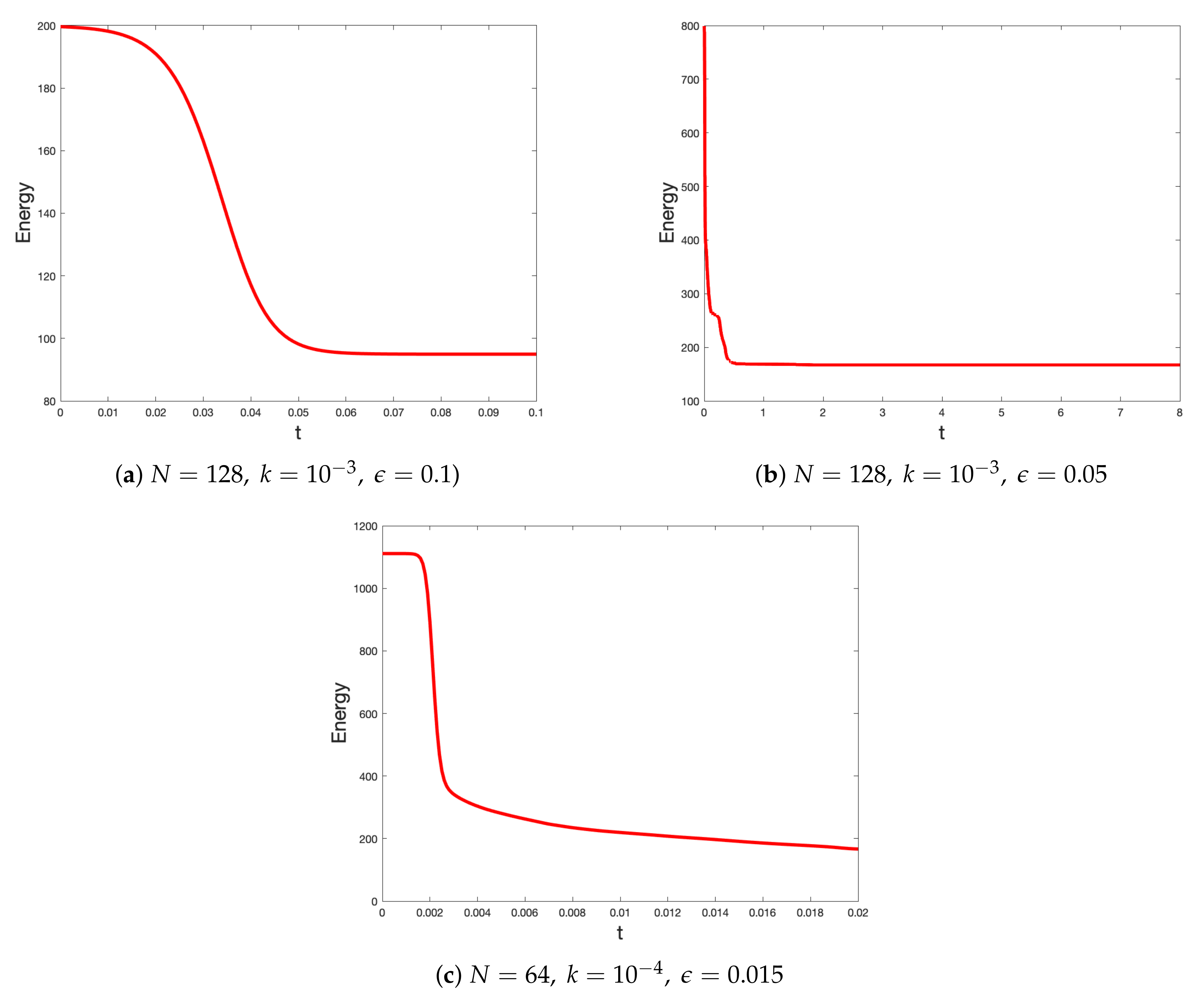
In order to further verify the effectiveness of the proposed method, we study the spinodal decomposition of the numerical solution of the AC Equation (1) with the following randomly perturbed distribution as the initial condition on the computational domain $\mathsf{\Omega }=[0,1]\times [0,1]\times [0,1]$:

$$\begin{array}{cc}\hfill & u_0(x,y,z)=0.005\mathrm{rand}(x,y,z),\hfill \end{array}$$

(9)

where rand $(x,y,z)$ is a random number between one and −1. A simulation was run up to the final time $T=2\times {10}^{-2}$ with $N=64,k={10}^{-4},\mathrm{and}ϵ=0.015$. Snapshots of the time evolution of the morphological patterns are summarized in Figure 5.

4.5. Stability Test

In Problems 1 to 4, we saw that the proposed method is indeed fourth-order accurate in the time direction to solve 1D, 2D, and 3D AC equations with different initial conditions. In order to show that the method is also gradient stable (that is, the energy $E\left(u\right)$ decays with time) [34], we plot the discrete Lyapunov energy:

$$\begin{array}{ccc}\hfill & E^h\left(u^n\right)=\frac{h^3}{4{ϵ}^2}\sum _{i=1}^N\sum _{j=1}^N\sum _{k=1}^N{({\left(u_{i,j,k}^n\right)}^2-1)}^2+\frac{h^3}{2}\sum _{j=1}^N\sum _{k=1}^N\sum _{i=2}^{N-1}{\left(\frac{u_{i+1,j,k}^n-u_{i-1,j,k}^n}{2h}\right)}^2+\hfill & \hfill \\ \hfill & \frac{h^3}{2}\sum _{i=1}^N\sum _{k=1}^N\sum _{j=2}^{N-1}{\left(\frac{u_{i,j+1,k}^n-u_{i,j-1,k}^n}{2h}\right)}^2+\frac{h^3}{2}\sum _{i=1}^N\sum _{j=1}^N\sum _{k=2}^{N-1}{\left(\frac{u_{i,j,k+1}^n-u_{i,j,k-1}^n}{2h}\right)}^2\hfill & \hfill \end{array}$$

(10)

obtained via the proposed method for the initial conditions: (8), (9), and:

$$\begin{array}{ccc}\hfill & u_0(x,y,z)=ϵ0.05cos\left(1.5\pi x\right)cos\left(1.5\pi y\right)\left(sin\left(2\pi z\right)+sin\left(\pi z\right)\right)\hfill & \hfill \end{array}$$

(11)

on the domain $\mathsf{\Omega }=[0,1]\times [0,1]\times [0,1]$. From Figure 6, we can see that the proposed method is able to reduce the energy in time. Moreover, it can be seen that the behavior of the energy diagrams in Figure 6 changes according to the imposed initial conditions and the values of the parameter $ϵ$.

Remark 5.

To the best of the authors’ knowledge, no theoretical energy stability analysis of the proposed method has been discussed to date, so we will address this interesting topic in our future work.

5. Conclusions

In this article, a strongly stable higher order time-stepping method combined with the Fourier spectral technique was proposed as an attractive and easy-to-implement alternative for integrating multi-dimensional AC equations. The proposed method utilized the discrete fast Fourier transform, which ensures efficiency and allows an extension of the stencil to 2D and 3D in a completely straightforward way and an easy implementation of various boundary conditions. A variety of numerical experiments were presented to confirm the accuracy and stability of the proposed method. In particular, the method was shown to be gradient stable (the method was able to satisfy the discrete energy law (10)) and fourth-order accurate in the time direction. It will be interesting to further theoretically investigate the energy stability of the proposed method and implement it on various modified forms of the AC equation such as crystal growth, grain growth, and image analysis.

References

1. Joshi, J. Existence and nonexistence of solutions for sublinear problems with prescribed number of zeros on exterior domains. Electron. J. Differ. Equ. 2017, 133, 1–10. [Google Scholar]
2. Joshi, J.; Iaia, J. Existence of solutions for semilinear problems with prescribed number of zeros on exterior domains. Electron. J. Differ. Equ. 2016, 112, 1–11. [Google Scholar]
3. Joshi, J.; Iaia, J. Infinitely many solutions for a semilinear problem on exterior domains with nonlinear boundary condition. Electron. J. Differ. Equ. 2018, 108, 1–10. [Google Scholar]
4. Allen, S.M.; Cahn, J.W. A microscopic theory for antiphase boundary motion and its application to antipahse domain coarsening. Acta Metall. 1979, 27, 1085–1095. [Google Scholar] [CrossRef]
5. Du, Q.; Liu, C.; Wang, X. A phase field approach in the numerical study of the elastic bending energy for vesicle membranes. J. Comput. Phys. 2004, 198, 450–468. [Google Scholar] [CrossRef]
6. Evans, L.C.; Sooner, H.M.; Souganidis, P.E. Phase transitions and generalized motion by mean curvature. Commun. Pure Appl. Math. 1992, 45, 1097–1123. [Google Scholar] [CrossRef]
7. Evans, L.C.; Spruck, J. Motion of level sets by mean curvature. I. J. Differ. Geom. 1991, 33, 635–681. [Google Scholar] [CrossRef]
8. Feng, X.B.; Prohl, A. Numerical analysis of the Allen–Cahn equation and approximation for mean curvature flows. Numer. Math. 2003, 94, 33–65. [Google Scholar] [CrossRef]
9. Liu, C.; Shen, J. A phase field model for the mixture of two incompressible fluids and its approximation by a Fourier-spectral method. Physica D 2003, 179, 211–228. [Google Scholar] [CrossRef] [Green Version]
10. Yang, X.; Feng, J.J.; Liu, C.; Shen, J. Numerical simulations of jet pinching-off and drop formation using an energetic variational phase-field method. J. Comput. Phys. 2006, 218, 417–428. [Google Scholar] [CrossRef]
11. Yue, P.; Zhou, C.; Feng, J.J.; Ollivier-Gooch, C.F.; Hu, H.H. Phase-field simulations of interfacial dynamics in viscoelastic fluids using finite elements with adaptive meshing. J. Comput. Phys. 2006, 219, 47–67. [Google Scholar] [CrossRef]
12. Yue, P.; Feng, J.J.; Liu, C.; Shen, J. Diffuse-interface simulations of drop coalescence and retraction in viscoelastic fluids. J. Non-Newtonian Fluid Mech. 2005, 129, 163–176. [Google Scholar] [CrossRef] [Green Version]
13. Choi, J.W.; Lee, H.G.; Jenog, D.; Kim, J. An unconditionally gradient stable numerical method for solving the Allen–Cahn equation. Physica A 2009, 388, 1791–1803. [Google Scholar] [CrossRef]
14. Lee, H.G.; Lee, J.Y. A semi-analytical Fourier spectral method for the Allen–Cahn equation. Comput. Math. Appl. 2014, 68, 174–184. [Google Scholar] [CrossRef]
15. Lee, H.G.; Lee, J.Y. A second order operator splitting method for Allen–Cahn type equations with nonlinear source terms. Physica A 2015, 432, 24–34. [Google Scholar] [CrossRef]
16. Li, Y.; Lee, H.G.; Jeong, D.; Kim, J. An unconditionally stable hybrid numerical method for solving the Allen–Cahn equation. Comput. Math. Appl. 2010, 60, 1591–1606. [Google Scholar] [CrossRef] [Green Version]
17. Peaceman, D.; Rachford, H. The numerical solution of parabolic and elliptic differential equations. J. Soc. Ind. Appl. Math. 1955, 3, 28–41. [Google Scholar] [CrossRef]
18. Shen, J.; Tang, T.; Yang, J. On the maximum principle preserving schemes for the generalized Allen–Cahn equation. Commun. Math. Sci. 2016, 14, 1517–1534. [Google Scholar] [CrossRef]
19. Tang, T.; Yang, J. Implicit-explicit scheme for the Allen–Cahn equation preserve the maximum principle. J. Comput. Math. 2016, 34, 451–461. [Google Scholar]
20. Yang, X. Error analysis of stabilized semi-implicit method of Allen–Cahn equation. Discret. Contin. Dyn. B 2009, 11, 1057–1070. [Google Scholar] [CrossRef]
21. Zhang, J.; Du, Q. Numerical studies of discrete approximations to the Allen–Cahn equation in the sharp interface limit. SIAM J. Sci. Comput. 2009, 31, 3042–3063. [Google Scholar] [CrossRef]
22. Argyros, I.K. Computational Theory of Iterative Methods; Series: Studies in Computational Mathematics; Elsevier Publication Company: New York, NY, USA, 2007. [Google Scholar]
23. Argyros, I.K.; Magrenan, A.A. Iterative Methods and Their Dynamics with Applications; CRC Press, Taylor and Francis: Boca Raton, FL, USA, 2017. [Google Scholar]
24. Bhatt, H.; Chowdhury, A. Comparative analysis of numerical methods for the multidimensional Brusselator system. Open J. Math. Sci. 2019, 3, 262–272. [Google Scholar] [CrossRef]
25. Gottlieb, S.; Wang, C. Stability and convergence analysis of fully discrete Fourier collocation spectral method for 3-D viscous Burgers’ equation. J. Sci. Comput. 2012, 53, 102–128. [Google Scholar] [CrossRef]
26. Cheng, K.; Wang, C. Long time stability of high order multi-step numerical schemes for two-dimensional incompressible Navier-Stokes equations. Siam J. Numer. Anal. 2016, 54, 3124–3144. [Google Scholar] [CrossRef] [Green Version]
27. Chen, W.; Li, W.; Wang, C.; Wang, S.; Wang, X. Energy stable higher-order linear ETD multi-step methods for gradient flows: Application to thin film epitaxy. Res. Math Sci. 2020, 7, 13. [Google Scholar] [CrossRef]
28. Yen, Y.; Chen, W.; Wang, C.; Wise, S.M. A second-order energy stable BDF numerical scheme for the Cahn-Hilliard Equation. Commun. Comput. Phys. 2018, 23, 572–602. [Google Scholar] [CrossRef] [Green Version]
29. Bueno-Orevo, A.; Kay, D.; Burrage, K. Fourier spectral methods for fractional-in-space reaction-diffusion equations. BIT 2014, 54, 937–954. [Google Scholar] [CrossRef]
30. Pindza, E.; Owolabi, K.M. Fourier spectral method for higher order space fractional reaction–diffusion equations. Comm. Nonlinear Sci. Numer. Simulat. 2016, 40, 112–128. [Google Scholar] [CrossRef] [Green Version]
31. Cox, S.M.; Matthews, P.C. Exponential time differencing for stiff systems. J. Comput. Phys. 2002, 176, 430–455. [Google Scholar] [CrossRef] [Green Version]
32. Bhatt, H.P.; Khaliq, A.Q.M. A compact fourth-order L-stable scheme for reaction-diffusion systems with nonsmooth data. J. Comput. Appl. Math. 2016, 299, 176–193. [Google Scholar] [CrossRef]
33. Ayub, S.; Affan, H.; Shah, A. Comparison of operator splitting schemes for numerical solutions of the Allen–Cahn equation. AIP Adv. 2019, 9, 125202-1–125202-9. [Google Scholar] [CrossRef] [Green Version]
34. Zhai, S.; Feng, X.; He, Y. Numerical simulation of the three dimensional Allen–Cahn equation by the high-order compact ADI method. Comput. Phys. Commun. 2014, 185, 2449–2455. [Google Scholar] [CrossRef]
Figure 1. The convergence rate of the Fourier spectral method for Problem 1.
Symmetry 13 00245 g001
Figure 2. (a) Comparison of exact and numerical solutions. (b) Traveling wave solution obtained via the proposed method.
Symmetry 13 00245 g002
Figure 3. Scenarios of the shrinking of the circle obtained via the proposed method at different times ( a ) t = 0 , ( b ) t = 0.0075 , ( c ) t = 0.015 , and ( d ) t = 0.0352 .
Symmetry 13 00245 g003
Figure 4. Space-time evolution profile of the star-shaped interface in a curvature-driven flow obtained via the proposed method with the parameters ϵ = 4 h 2 2 tanh 1 ( 0.9 ) , k = 10 5 , and N = 128 at various times.
Symmetry 13 00245 g004
Figure 5. Spinodal decomposition of the numerical solution using the proposed method with h = 1 64 , k = 10 4 , and ϵ = 0.015 at different times.
Symmetry 13 00245 g005
Figure 6. Energy diagrams (a,b) with the initial conditions (8) and (11) for Problem 3 and (c) with the initial condition (9) for Problem 4.
Symmetry 13 00245 g006