
An Improved Transient Search Optimization with Neighborhood Dimensional Learning for Global Optimization Problems


Abstract
1. Introduction
2. Transient Search Algorithm
2.1. Background Information
2.2. Mathematical Models
| Algorithm 1: TSO |
| Input: Number of Search Agents: N; Dimension: d; Maximum number of iterations: Max_iter |
| Output: The global optimum |
| Generate initial populations by the Equation (5) |
| Calculating the fitness value of the population |
| Filter the best search agent’s fitness value and location |
| Whilet < Max_iter |
| Calculating the value of T and by the Equations (7) and (8) |
| If |
| Update the location of the search agent by the Equation (6) |
| Else if |
| Update the location of the search agent by the Equation (10) |
| End if |
| Calculating the fitness value of the population |
| Update optimal search agent position and fitness |
| End while |
3. Improved Transient Search Algorithm
3.1. Chaotic Opposition Learning
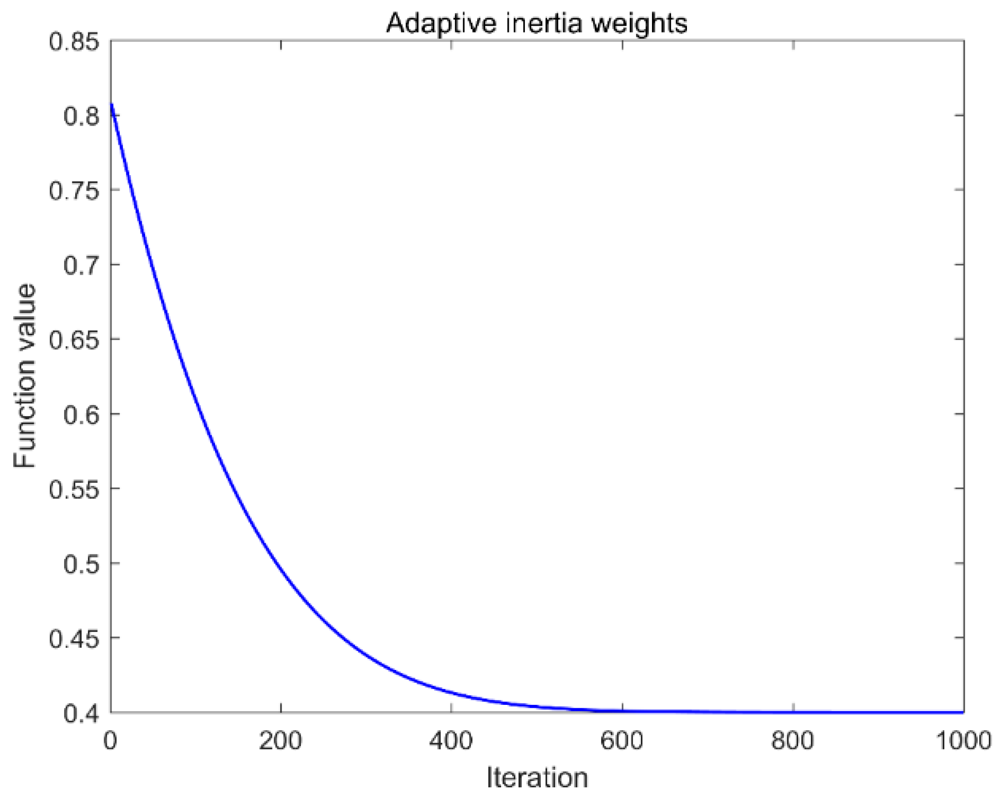
3.2. Adaptive Inertia Weights
3.3. Neighborhood Dimensional Learning
| Algorithm 2: ITSO |
| Input: Number of Search Agents: N; Dimension: d; Maximum number of iterations: Max_iter |
| Output: The global optimum |
| Generate chaotic tent mapping sequences by the Equation (11) |
| Initialized populations by the Equation (12) |
| Generation of Opposing Populations by the Equation (13) |
| Calculate the fitness values of the alternative populations. |
| The first N with good fitness values are selected as the initial populations |
| Whilet < Max_iter |
| Calculating Adaptive Inertia Weights by the Equation (14) |
| Calculating the value of T and by the Equations (7) and (8) |
| If |
| Update the location of the search agent by the Equation (15) |
| Else if |
| Update the location of the search agent by the Equation (16) |
| End if |
| Generation of candidate populations by the Equation (17) |
| Calculating Neighborhood Radius by the Equation (18) |
| Finding Neighborhood Populations by the Equation (19) |
| Calculation of NDL populations by the Equation (20) |
| Calculate fitness values to update population position by the Equation (21) |
| Update optimal search agent position and fitness |
| End while |
4. Simulation Experiments and Comparative Analysis
4.1. Experimental Settings
4.2. Benchmark Function
4.3. Experimental Results and Analysis
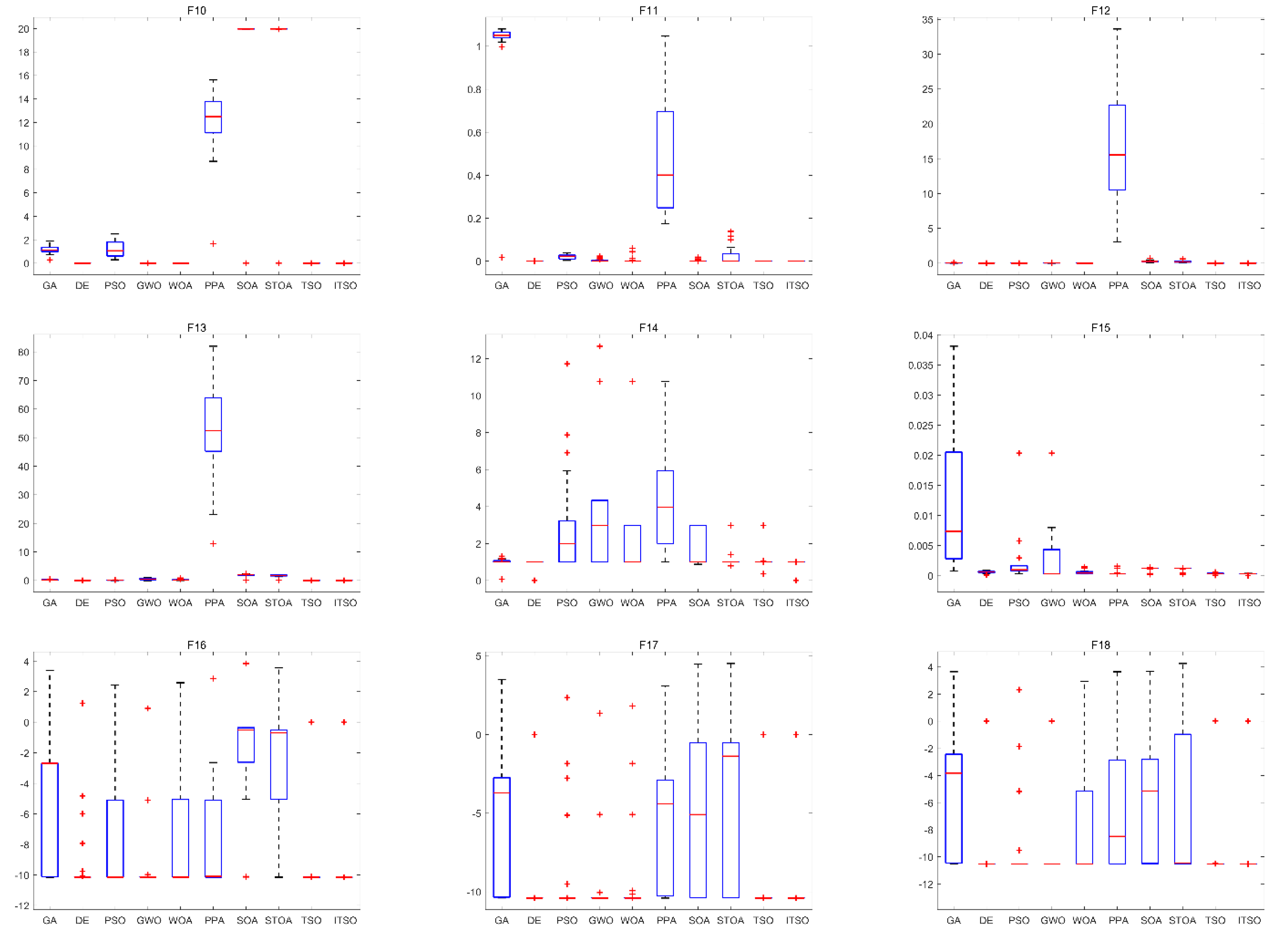
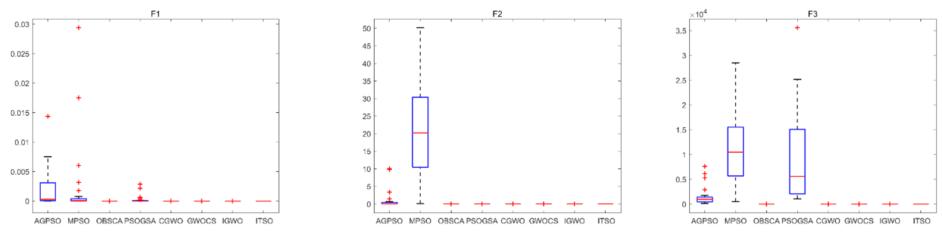
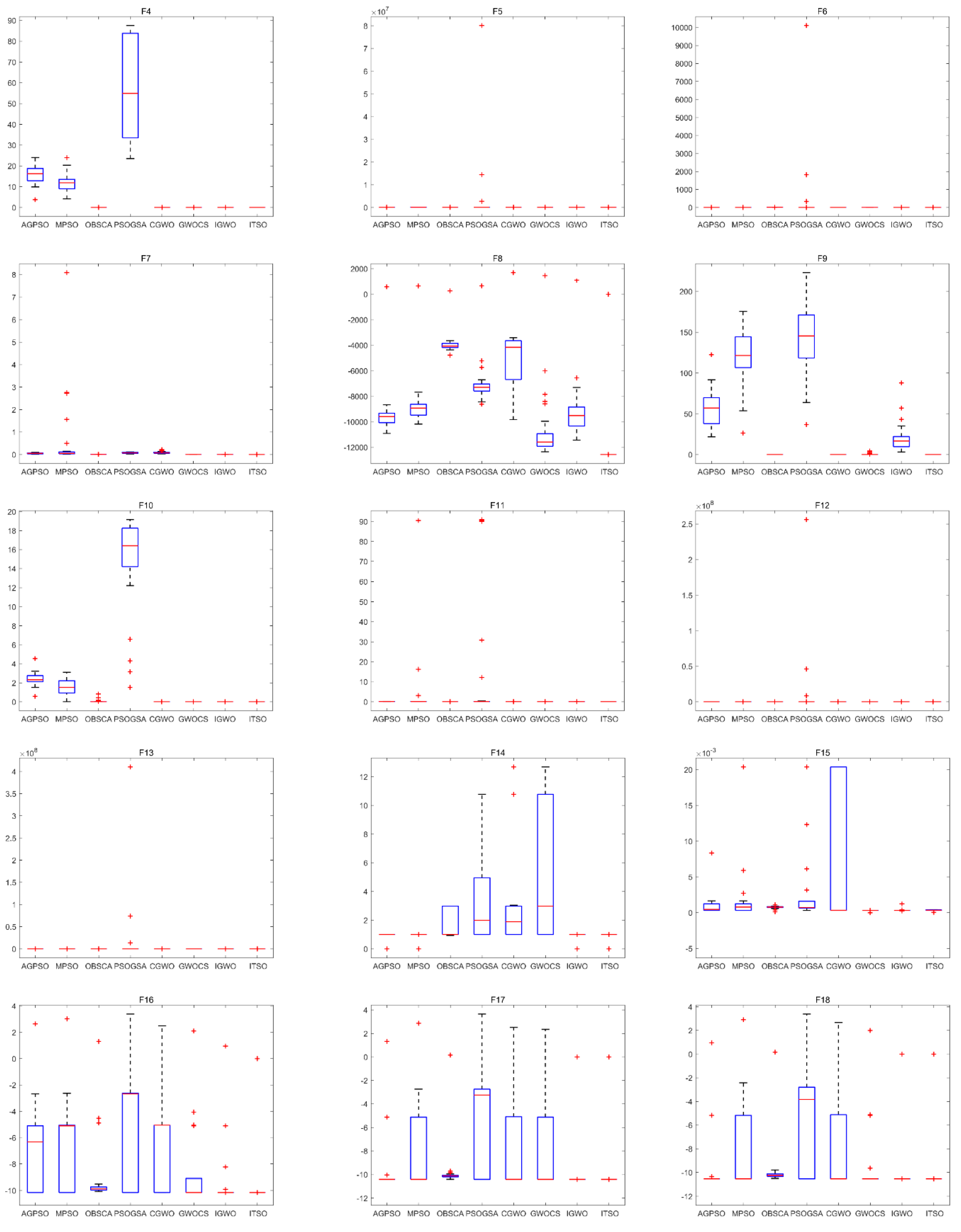
4.4. Algorithm Stability Analysis
4.5. Wilcoxon’s Rank Sum Test Analysis
4.6. High-Dimensional Performance Analysis
5. Conclusions
Author Contributions
Funding
Data Availability Statement
Conflicts of Interest
References
- Adarsh, B.R.; Raghunathan, T.; Jayabarathi, T.; Yang, X.-S. Economic Dispatch Using Chaotic Bat Algorithm. Energy 2016, 96, 666–675. [Google Scholar] [CrossRef]
- Jayabarathi, T.; Raghunathan, T.; Adarsh, B.R.; Suganthan, P.N. Economic Dispatch Using Hybrid Grey Wolf Optimizer. Energy 2016, 111, 630–641. [Google Scholar] [CrossRef]
- Kuo, R.J.; Hong, C.W. Integration of Genetic Algorithm and Particle Swarm Optimization for Investment Portfolio Optimization. Appl. Math. Inf. Sci. 2013, 7, 2397–2408. [Google Scholar] [CrossRef]
- Haghofer, A.; Dorl, S.; Oszwald, A.; Breuss, J.; Jacak, J.; Winkler, S.M. Evolutionary Optimization of Image Processing for Cell Detection in Microscopy Images. Soft Comput. 2020, 24, 17847–17862. [Google Scholar] [CrossRef]
- Qiao, L.; Wang, Z.; Wang, Y.; Zhu, J. Mechanical Performance-Based Optimum Design of High Carbon Pearlitic Steel by Particle Swarm Optimization. Steel Res. Int. 2021, 92, 2000252. [Google Scholar] [CrossRef]
- Kalathingal, M.S.H.; Basak, S.; Mitra, J. Artificial Neural Network Modeling and Genetic Algorithm Optimization of Process Parameters in Fluidized Bed Drying of Green Tea Leaves. J. Food Process Eng. 2020, 43, e13128. [Google Scholar] [CrossRef]
- Yang, L.; Chen, H. Fault Diagnosis of Gearbox Based on RBF-PF and Particle Swarm Optimization Wavelet Neural Network. Neural Comput. Appl. 2019, 31, 4463–4478. [Google Scholar] [CrossRef]
- Hemeida, A.M.; Alkhalaf, S.; Mady, A.; Mahmoud, E.A.; Hussein, M.E.; Baha Eldin, A.M. Implementation of Nature-Inspired Optimization Algorithms in Some Data Mining Tasks. Ain Shams Eng. J. 2020, 11, 309–318. [Google Scholar] [CrossRef]
- Martens, D.; Baesens, B.; Fawcett, T. Editorial Survey: Swarm Intelligence for Data Mining. Mach. Learn. 2011, 82, 1–42. [Google Scholar] [CrossRef]
- Hu, Q.; Xie, Y.; Zhang, Z. Modification of Breakthrough Models in a Continuous-Flow Fixed-Bed Column: Mathematical Characteristics of Breakthrough Curves and Rate Profiles. Sep. Purif. Technol. 2020, 238, 116399. [Google Scholar] [CrossRef]
- Jafari, S.; Nikolaidis, T. Meta-Heuristic Global Optimization Algorithms for Aircraft Engines Modelling and Controller Design; A Review, Research Challenges, and Exploring the Future. Prog. Aerosp. Sci. 2019, 104, 40–53. [Google Scholar] [CrossRef]
- Nadimi-Shahraki, M.H.; Taghian, S.; Mirjalili, S. An Improved Grey Wolf Optimizer for Solving Engineering Problems. Expert Syst. Appl. 2021, 166, 113917. [Google Scholar] [CrossRef]
- Yang, X.S.; Gandomi, A.H. Bat Algorithm: A Novel Approach for Global Engineering Optimization. Eng. Comput. (Swans. Wales) 2012. [Google Scholar] [CrossRef]
- Gao, K.; Cao, Z.; Zhang, L.; Chen, Z.; Han, Y.; Pan, Q. A Review on Swarm Intelligence and Evolutionary Algorithms for Solving Flexible Job Shop Scheduling Problems. IEEE/CAA J. Autom. Sin. 2019, 6, 904–916. [Google Scholar] [CrossRef]
- Munk, D.J.; Vio, G.A.; Steven, G.P. Topology and Shape Optimization Methods Using Evolutionary Algorithms: A Review. Struct. Multidisc. Optim. 2015, 52, 613–631. [Google Scholar] [CrossRef]
- Albadr, M.A.; Tiun, S.; Ayob, M.; AL-Dhief, F. Genetic Algorithm Based on Natural Selection Theory for Optimization Problems. Symmetry 2020, 12, 1758. [Google Scholar] [CrossRef]
- Mallipeddi, R.; Suganthan, P.N.; Pan, Q.K.; Tasgetiren, M.F. Differential Evolution Algorithm with Ensemble of Parameters and Mutation Strategies. Appl. Soft Comput. 2011, 11, 1679–1696. [Google Scholar] [CrossRef]
- Eriksson, R.; Olsson, B. Adapting Genetic Regulatory Models by Genetic Programming. Biosystems 2004, 76, 217–227. [Google Scholar] [CrossRef]
- Li, K.; Gu, F.; Li, W.; Huang, Y. A Dual-Population Evolutionary Algorithm Adapting to Complementary Evolutionary Strategy. Int. J. Patt. Recogn. Artif. Intell. 2019, 33, 1959004. [Google Scholar] [CrossRef]
- Aljarah, I.; Faris, H.; Mirjalili, S.; Al-Madi, N. Training Radial Basis Function Networks Using Biogeography-Based Optimizer. Neural Comput. Appl. 2018, 29, 529–553. [Google Scholar] [CrossRef]
- Basu, M. Fast Convergence Evolutionary Programming for Economic Dispatch Problems. IET Gener. Transm. Distrib. 2017, 11, 4009–4017. [Google Scholar] [CrossRef]
- Brezočnik, L.; Fister, I.; Podgorelec, V. Swarm Intelligence Algorithms for Feature Selection: A Review. Appl. Sci. 2018, 8, 1521. [Google Scholar] [CrossRef]
- Tian, D.; Hu, J.; Sheng, Z.; Wang, Y.; Ma, J.; Wang, J. Swarm Intelligence Algorithm Inspired by Route Choice Behavior. J. Bionic Eng. 2016, 13, 669–678. [Google Scholar] [CrossRef]
- Esmin, A.A.A.; Coelho, R.A.; Matwin, S. A Review on Particle Swarm Optimization Algorithm and Its Variants to Clustering High-Dimensional Data. Artif. Intell. Rev. 2015, 44, 23–45. [Google Scholar] [CrossRef]
- Afshar, A.; Massoumi, F.; Afshar, A.; Mariño, M.A. State of the Art Review of Ant Colony Optimization Applications in Water Resource Management. Water Resour. Manag. 2015, 29, 3891–3904. [Google Scholar] [CrossRef]
- Mirjalili, S.; Lewis, A. The Whale Optimization Algorithm. Adv. Eng. Softw. 2016, 95, 51–67. [Google Scholar] [CrossRef]
- Faramarzi, A.; Heidarinejad, M.; Mirjalili, S.; Gandomi, A.H. Marine Predators Algorithm: A Nature-Inspired Metaheuristic. Expert Syst. Appl. 2020, 152, 113377. [Google Scholar] [CrossRef]
- Mirjalili, S.; Mirjalili, S.M.; Yang, X.-S. Binary Bat Algorithm. Neural Comput. Appl. 2014, 25, 663–681. [Google Scholar] [CrossRef]
- Wang, G.-G.; Deb, S.; Gandomi, A.H.; Zhang, Z.; Alavi, A.H. Chaotic Cuckoo Search. Soft Comput. 2016, 20, 3349–3362. [Google Scholar] [CrossRef]
- Banitalebi, A.; Aziz, M.I.A.; Bahar, A.; Aziz, Z.A. Enhanced Compact Artificial Bee Colony. Inf. Sci. 2015, 298, 491–511. [Google Scholar] [CrossRef]
- Joshi, H.; Arora, S. Enhanced Grey Wolf Optimization Algorithm for Global Optimization. Fundam. Inform. 2017, 153, 235–264. [Google Scholar] [CrossRef]
- Dhiman, G.; Kumar, V. Seagull Optimization Algorithm: Theory and Its Applications for Large-Scale Industrial Engineering Problems. Knowl. Based Syst. 2019, 165, 169–196. [Google Scholar] [CrossRef]
- Chin, V.J.; Salam, Z. Coyote Optimization Algorithm for the Parameter Extraction of Photovoltaic Cells. Sol. Energy 2019, 194, 656–670. [Google Scholar] [CrossRef]
- Dhiman, G.; Kaur, A. STOA: A Bio-Inspired Based Optimization Algorithm for Industrial Engineering Problems. Eng. Appl. Artif. Intell. 2019, 82, 148–174. [Google Scholar] [CrossRef]
- Kaveh, A.; Vaez, S.R.H.; Hosseini, P. Simplified Dolphin Echolocation Algorithm for Optimum Design of Frame. Smart Struct. Syst. 2018, 21, 321–333. [Google Scholar] [CrossRef]
- Wang, G.-G.; Gandomi, A.H.; Alavi, A.H. Stud Krill Herd Algorithm. Neurocomputing 2014, 128, 363–370. [Google Scholar] [CrossRef]
- Harifi, S.; Khalilian, M.; Mohammadzadeh, J.; Ebrahimnejad, S. Optimizing a Neuro-Fuzzy System Based on Nature-Inspired Emperor Penguins Colony Optimization Algorithm. IEEE Trans. Fuzzy Syst. 2020, 28, 1110–1124. [Google Scholar] [CrossRef]
- Mohamed, A.-A.A.; Hassan, S.A.; Hemeida, A.M.; Alkhalaf, S.; Mahmoud, M.M.M.; Baha Eldin, A.M. Parasitism–Predation Algorithm (PPA): A Novel Approach for Feature Selection. Ain Shams Eng. J. 2019, 11, 293–308. [Google Scholar] [CrossRef]
- Kogan, G.; Klein, R.; Bortman, J. A Physics-Based Algorithm for the Estimation of Bearing Spall Width Using Vibrations. Mech. Syst. Signal Process. 2018, 104, 398–414. [Google Scholar] [CrossRef]
- Bozorg-Haddad, O.; Janbaz, M.; Loáiciga, H.A. Application of the Gravity Search Algorithm to Multi-Reservoir Operation Optimization. Adv. Water Resour. 2016, 98, 173–185. [Google Scholar] [CrossRef]
- Kaveh, A.; Talatahari, S. A Novel Heuristic Optimization Method: Charged System Search. Acta Mech. 2010, 213, 267–289. [Google Scholar] [CrossRef]
- Kaveh, A.; Khayatazad, M. Ray Optimization for Size and Shape Optimization of Truss Structures. Comput. Struct. 2013, 117, 82–94. [Google Scholar] [CrossRef]
- Erol, O.K.; Eksin, I. A New Optimization Method: Big Bang–Big Crunch. Adv. Eng. Softw. 2006, 37, 106–111. [Google Scholar] [CrossRef]
- Zhao, W.; Wang, L.; Zhang, Z. A Novel Atom Search Optimization for Dispersion Coefficient Estimation in Groundwater. Future Gener. Comput. Syst. 2019, 91, 601–610. [Google Scholar] [CrossRef]
- Hashim, F.A.; Houssein, E.H.; Mabrouk, M.S.; Al-Atabany, W.; Mirjalili, S. Henry Gas Solubility Optimization: A Novel Physics-Based Algorithm. Future Gener. Comput. Syst. 2019, 101, 646–667. [Google Scholar] [CrossRef]
- Lockett, A.J.; Miikkulainen, R. A Probabilistic Reformulation of No Free Lunch: Continuous Lunches Are Not Free. Evol. Comput. 2017, 25, 503–528. [Google Scholar] [CrossRef]
- Qais, M.H.; Hasanien, H.M.; Alghuwainem, S. Transient Search Optimization: A New Meta-Heuristic Optimization Algorithm. Appl. Intell. 2020, 50, 3926–3941. [Google Scholar] [CrossRef]
- Qais, M.H.; Hasanien, H.M.; Alghuwainem, S. Transient Search Optimization for Electrical Parameters Estimation of Photovoltaic Module Based on Datasheet Values. Energy Convers. Manag. 2020, 214, 112904. [Google Scholar] [CrossRef]
- Dashtipour, K.; Gogate, M.; Li, J.; Jiang, F.; Kong, B.; Hussain, A. A Hybrid Persian Sentiment Analysis Framework: Integrating Dependency Grammar Based Rules and Deep Neural Networks. Neurocomputing 2020, 380, 1–10. [Google Scholar] [CrossRef]
- Yang, X.S. Review of Meta-Heuristics and Generalised Evolutionary Walk Algorithm. IJBIC 2011, 3, 77. [Google Scholar] [CrossRef]
- Mirjalili, S.; Lewis, A.; Sadiq, A.S. Autonomous Particles Groups for Particle Swarm Optimization. Arab. J. Sci. Eng. 2014, 39, 4683–4697. [Google Scholar] [CrossRef]
- Zhou, H.; Pang, J.; Chen, P.-K.; Chou, F.-D. A Modified Particle Swarm Optimization Algorithm for a Batch-Processing Machine Scheduling Problem with Arbitrary Release Times and Non-Identical Job Sizes. Comput. Ind. Eng. 2018, 123, 67–81. [Google Scholar] [CrossRef]
- Abd Elaziz, M.; Oliva, D.; Xiong, S. An Improved Opposition-Based Sine Cosine Algorithm for Global Optimization. Expert Syst. Appl. 2017, 90, 484–500. [Google Scholar] [CrossRef]
- Meshram, S.G.; Ghorbani, M.A.; Shamshirband, S.; Karimi, V.; Meshram, C. River Flow Prediction Using Hybrid PSOGSA Algorithm Based on Feed-Forward Neural Network. Soft Comput. 2019, 23, 10429–10438. [Google Scholar] [CrossRef]
- Kohli, M.; Arora, S. Chaotic Grey Wolf Optimization Algorithm for Constrained Optimization Problems. J. Comput. Des. Eng. 2018, 5, 458–472. [Google Scholar] [CrossRef]
- Long, W.; Cai, S.; Jiao, J.; Xu, M.; Wu, T. A New Hybrid Algorithm Based on Grey Wolf Optimizer and Cuckoo Search for Parameter Extraction of Solar Photovoltaic Models. Energy Convers. Manag. 2020, 203, 112243. [Google Scholar] [CrossRef]
- Sayed, G.I.; Khoriba, G.; Haggag, M.H. A Novel Chaotic Salp Swarm Algorithm for Global Optimization and Feature Selection. Appl. Intell. 2018, 48, 3462–3481. [Google Scholar] [CrossRef]
- Han, C. An Image Encryption Algorithm Based on Modified Logistic Chaotic Map. Optik 2019, 181, 779–785. [Google Scholar] [CrossRef]
- Tubishat, M.; Idris, N.; Shuib, L.; Abushariah, M.A.M.; Mirjalili, S. Improved Salp Swarm Algorithm Based on Opposition Based Learning and Novel Local Search Algorithm for Feature Selection. Expert Syst. Appl. 2020, 145, 113122. [Google Scholar] [CrossRef]
- Taherkhani, M.; Safabakhsh, R. A Novel Stability-Based Adaptive Inertia Weight for Particle Swarm Optimization. Appl. Soft Comput. 2016, 38, 281–295. [Google Scholar] [CrossRef]
- Mirjalili, S.; Mirjalili, S.M.; Lewis, A. Grey Wolf Optimizer. Adv. Eng. Softw. 2014. [Google Scholar] [CrossRef]
- Derrac, J.; García, S.; Molina, D.; Herrera, F. A Practical Tutorial on the Use of Nonparametric Statistical Tests as a Methodology for Comparing Evolutionary and Swarm Intelligence Algorithms. Swarm Evol. Comput. 2011, 1, 3–18. [Google Scholar] [CrossRef]
- Chen, H.; Li, W.; Yang, X. A Whale Optimization Algorithm with Chaos Mechanism Based on Quasi-Opposition for Global Optimization Problems. Expert Syst. Appl. 2020, 158, 113612. [Google Scholar] [CrossRef]


| Algorithm | Parameter Specific Settings |
|---|---|
| GA | |
| DE | |
| PSO | , |
| GWO | |
| WOA | |
| PPA | , |
| SOA | , Control Parameter (A) ∈ [2, 0] |
| STOA | |
| AGPSO | , |
| MPSO | , , |
| OBSCA | , |
| PSOGSA | , , |
| CGWO | , , |
| GWOCS | , |
| IGWO | |
| TSO | , |
| ITSO | , |
| Type | Function | Dim | Range | Optimum Value |
|---|---|---|---|---|
| Unimodal | 50 | [−100, 100] | 0 | |
| Unimodal | 50 | [−10, 10] | 0 | |
| Unimodal | 50 | [−100, 100] | 0 | |
| Unimodal | 50 | [−100, 100] | 0 | |
| Unimodal | 50 | [−30, 30] | 0 | |
| Unimodal | 50 | [−100, 100] | 0 | |
| Unimodal | 50 | [−1.28, 1.28] | 0 | |
| Multimodal | 50 | [−500, 500] | −418.9829 × d | |
| Multimodal | 50 | [−5.12, 5.12] | 0 | |
| Multimodal | 50 | [−32, 32] | 0 | |
| Multimodal | 50 | [−600, 600] | 0 | |
| Multimodal | 50 | [−50, 50] | 0 | |
| Multimodal | 50 | [−50, 50] | 0 | |
| Fixed Dimension | 2 | [−65, 65] | 1 | |
| Fixed Dimension | 4 | [−5, 5] | 0.00030 | |
| Fixed Dimension | 4 | [0, 10] | −10.1532 | |
| Fixed Dimension | 4 | [0, 10] | −10.4028 | |
| Fixed Dimension | 4 | [0, 10] | −10.5363 |
| Function | Criteria | ITSO | TSO | PSO | GWO | WOA | PPA | SOA | STOA | GA | DE |
|---|---|---|---|---|---|---|---|---|---|---|---|
| F1 | Ave | 0.00 × 10+00 | 2.44 × 10−201 | 3.15 × 10−01 | 4.65 × 10−59 | 9.93 × 10−149 | 1.22 × 10+00 | 1.24 × 10⁻²⁷ | 1.94 × 10⁻¹⁷ | 5.88 × 10+00 | 7.03 × 10⁻¹¹ |
| Std | 0.00 × 10+00 | 0.00 × 10+00 | 2.00 × 10−01 | 1.02 × 10−58 | 5.32 × 10−148 | 2.52 × 10+00 | 2.00 × 10⁻²⁷ | 7.83 × 10⁻¹⁷ | 2.65 × 10+00 | 4.48 × 10⁻¹¹ | |
| Max | 0.00 × 10+00 | 7.32 × 10−200 | 9.19 × 10−01 | 5.53 × 10−58 | 2.96 × 10−147 | 1.39 × 10+01 | 6.91 × 10⁻²⁷ | 4.38 × 10⁻¹⁶ | 1.35 × 10+01 | 1.97 × 10⁻¹⁰ | |
| Min | 0.00 × 10+00 | 6.19 × 10−301 | 9.08 × 10−02 | 1.12 × 10−61 | 2.23 × 10−169 | 5.42 × 10−02 | 1.84 × 10⁻³¹ | 1.20 × 10⁻²⁰ | 1.82 × 10+00 | 9.07 × 10⁻¹² | |
| F2 | Ave | 0.00 × 10+00 | 4.22 × 10−102 | 8.74 × 10+00 | 9.87 × 10⁻³⁵ | 6.40 × 10−101 | 3.57 × 10+00 | 6.23 × 10⁻¹⁸ | 3.44 × 10⁻¹² | 8.63 × 10−01 | 2.80 × 10−07 |
| Std | 0.00 × 10+00 | 2.27 × 10−101 | 8.22 × 10+00 | 1.11 × 10⁻³⁴ | 3.45 × 10−100 | 2.60 × 10+00 | 7.38 × 10⁻¹⁸ | 7.09 × 10⁻¹² | 1.64 × 10−01 | 8.12 × 10−08 | |
| Max | 0.00 × 10+00 | 1.26 × 10−100 | 3.06 × 10+01 | 5.20 × 10⁻³⁴ | 1.92 × 10−99 | 1.01 × 10+01 | 3.54 × 10⁻¹⁷ | 3.91 × 10⁻¹¹ | 1.21 × 10+00 | 4.65 × 10−07 | |
| Min | 0.00 × 10+00 | 4.43 × 10−138 | 3.98 × 10−01 | 5.18 × 10−36 | 1.58 × 10−114 | 5.16 × 10−01 | 2.27 × 10⁻¹⁹ | 2.57 × 10⁻¹⁴ | 5.94 × 10−01 | 1.39 × 10−07 | |
| F3 | Ave | 0.00 × 10+00 | 4.15 × 10−84 | 7.65 × 10+01 | 2.67 × 10⁻¹⁴ | 2.41 × 10+04 | 4.61 × 10+02 | 2.03 × 10⁻¹² | 1.06 × 10−07 | 1.22 × 10+04 | 2.73 × 10+04 |
| Std | 0.00 × 10+00 | 2.24 × 10−83 | 1.59 × 10+01 | 8.37 × 10⁻¹⁴ | 1.20 × 10+04 | 2.36 × 10+02 | 7.43 × 10⁻¹² | 1.94 × 10−07 | 2.64 × 10+03 | 3.38 × 10+03 | |
| Max | 0.00 × 10+00 | 1.25 × 10−82 | 1.16 × 10+02 | 3.49 × 10⁻¹³ | 5.20 × 10+04 | 1.02 × 10+03 | 3.79 × 10⁻¹¹ | 7.31 × 10−07 | 1.85 × 10+04 | 3.64 × 10+04 | |
| Min | 0.00 × 10+00 | 3.35 × 10−239 | 3.60 × 10+01 | 2.48 × 10⁻²⁰ | 3.23 × 10+03 | 1.15 × 10+02 | 3.02 × 10⁻¹⁸ | 2.43 × 10⁻¹¹ | 8.23 × 10+03 | 2.12 × 10+04 | |
| F4 | Ave | 0.00 × 10+00 | 1.57 × 10−100 | 1.53 × 10+00 | 1.02 × 10⁻¹⁴ | 3.79 × 10+01 | 3.69 × 10+01 | 2.46 × 10−07 | 2.22 × 10−05 | 7.65 × 10+00 | 2.43 × 10+00 |
| Std | 0.00 × 10+00 | 8.32 × 10−100 | 2.31 × 10−01 | 1.36 × 10⁻¹⁴ | 3.17 × 10+01 | 8.45 × 10+00 | 9.90 × 10−07 | 2.22 × 10−05 | 1.28 × 10+00 | 3.85 × 10−01 | |
| Max | 0.00 × 10+00 | 4.64 × 10−99 | 2.08 × 10+00 | 6.20 × 10⁻¹⁴ | 9.00 × 10+01 | 5.61 × 10+01 | 5.54 × 10−06 | 6.81 × 10−05 | 1.07 × 10+01 | 3.33 × 10+00 | |
| Min | 0.00 × 10+00 | 1.44 × 10−135 | 1.05 × 10+00 | 7.56 × 10⁻¹⁶ | 1.52 × 10−01 | 2.37 × 10+01 | 3.63 × 10⁻¹¹ | 1.26 × 10−06 | 5.27 × 10+00 | 1.58 × 10+00 | |
| F5 | Ave | 2.18 × 10−04 | 2.83 × 10−02 | 4.01 × 10+02 | 2.70 × 10+01 | 2.72 × 10+01 | 3.69 × 10+02 | 2.80 × 10+01 | 2.79 × 10+01 | 4.55 × 10+02 | 5.26 × 10+01 |
| Std | 4.10 × 10−04 | 3.56 × 10−02 | 5.47 × 10+02 | 7.39 × 10−01 | 5.75 × 10−01 | 2.29 × 10+02 | 6.22 × 10−01 | 6.48 × 10−01 | 5.53 × 10+02 | 2.95 × 10+01 | |
| Max | 1.98 × 10−03 | 1.54 × 10−01 | 3.21 × 10+03 | 2.86 × 10+01 | 2.87 × 10+01 | 1.12 × 10+03 | 2.89 × 10+01 | 2.88 × 10+01 | 2.89 × 10+03 | 1.20 × 10+02 | |
| Min | 5.28 × 10−07 | 1.24 × 10−05 | 1.07 × 10+02 | 2.52 × 10+01 | 2.63 × 10+01 | 5.28 × 10+01 | 2.69 × 10+01 | 2.69 × 10+01 | 1.61 × 10+02 | 2.56 × 10+01 | |
| F6 | Ave | 5.53 × 10−06 | 6.77 × 10−04 | 2.93 × 10−01 | 6.26 × 10−01 | 6.37 × 10−02 | 8.35 × 10−01 | 3.19 × 10+00 | 2.60 × 10+00 | 5.51 × 10+00 | 2.18 × 10−03 |
| Std | 7.68 × 10−06 | 1.07 × 10−03 | 1.69 × 10−01 | 3.40 × 10−01 | 9.28 × 10−02 | 9.39 × 10−01 | 4.14 × 10−01 | 4.72 × 10−01 | 2.13 × 10+00 | 9.02 × 10−04 | |
| Max | 3.11 × 10−05 | 5.26 × 10−03 | 6.82 × 10−01 | 1.26 × 10+00 | 4.57 × 10−01 | 4.22 × 10+00 | 3.93 × 10+00 | 3.49 × 10+00 | 1.11 × 10+01 | 4.69 × 10−03 | |
| Min | 4.73 × 10−08 | 1.08 × 10−07 | 7.62 × 10−02 | 1.79 × 10−05 | 1.03 × 10−02 | 3.76 × 10−02 | 2.00 × 10+00 | 1.29 × 10+00 | 2.57 × 10+00 | 7.92 × 10−04 | |
| F7 | Ave | 1.93 × 10−04 | 9.56 × 10−05 | 8.19 × 10+00 | 9.88 × 10−04 | 1.32 × 10−03 | 3.79 × 10−01 | 9.09 × 10−04 | 1.57 × 10−03 | 1.12 × 10−01 | 3.00 × 10−02 |
| Std | 1.41 × 10−04 | 6.44 × 10−05 | 7.40 × 10+00 | 5.38 × 10−04 | 1.68 × 10−03 | 2.24 × 10−01 | 6.35 × 10−04 | 1.09 × 10−03 | 3.38 × 10−02 | 6.30 × 10−03 | |
| Max | 6.89 × 10−04 | 2.31 × 10−04 | 2.72 × 10+01 | 2.22 × 10−03 | 6.59 × 10−03 | 1.18 × 10+00 | 2.87 × 10−03 | 5.88 × 10−03 | 1.84 × 10−01 | 4.08 × 10−02 | |
| Min | 3.33 × 10−05 | 2.28 × 10−06 | 3.05 × 10−01 | 1.82 × 10−04 | 5.75 × 10−06 | 1.07 × 10−01 | 1.63 × 10−04 | 4.57 × 10−04 | 5.38 × 10−02 | 1.82 × 10−02 | |
| F8 | Ave | −1.26 × 10+04 | −1.26 × 10+04 | −6.51 × 10+03 | −6.18 × 10+03 | −1.12 × 10+04 | −8.02 × 10+03 | −5.48 × 10+03 | −5.59 × 10+03 | −1.26 × 10+04 | −1.24 × 10+04 |
| Std | 1.58 × 10−02 | 7.02 × 10−03 | 1.02 × 10+03 | 6.39 × 10+02 | 1.55 × 10+03 | 7.82 × 10+02 | 7.18 × 10+02 | 7.09 × 10+02 | 6.66 × 10+00 | 1.34 × 10+02 | |
| Max | −1.26 × 10+04 | −1.26 × 10+04 | −3.74 × 10+03 | −4.91 × 10+03 | −8.12 × 10+03 | −6.25 × 10+03 | −4.59 × 10+03 | −4.43 × 10+03 | −1.25 × 10+04 | −1.21 × 10+04 | |
| Min | −1.26 × 10+04 | −1.26 × 10+04 | −8.17 × 10+03 | −7.22 × 10+03 | −1.26 × 10+04 | −9.61 × 10+03 | −7.10 × 10+03 | −8.19 × 10+03 | −1.26 × 10+04 | −1.26 × 10+04 | |
| F9 | Ave | 0.00 × 10+00 | 0.00 × 10+00 | 1.71 × 10+02 | 1.71 × 10⁻¹⁴ | 0.00 × 10+00 | 6.22 × 10+01 | 1.77 × 10+00 | 5.21 × 10+00 | 2.59 × 10+00 | 6.28 × 10+01 |
| Std | 0.00 × 10+00 | 0.00 × 10+00 | 3.82 × 10+01 | 2.60 × 10⁻¹⁴ | 0.00 × 10+00 | 1.84 × 10+01 | 5.44 × 10+00 | 1.94 × 10+01 | 8.73 × 10−01 | 6.07 × 10+00 | |
| Max | 0.00 × 10+00 | 0.00 × 10+00 | 2.44 × 10+02 | 5.68 × 10⁻¹⁴ | 0.00 × 10+00 | 9.75 × 10+01 | 2.35 × 10+01 | 1.04 × 10+02 | 4.85 × 10+00 | 7.32 × 10+01 | |
| Min | 0.00 × 10+00 | 0.00 × 10+00 | 9.55 × 10+01 | 0.00 × 10+00 | 0.00 × 10+00 | 3.68 × 10+01 | 0.00 × 10+00 | 5.68 × 10⁻¹⁴ | 1.40 × 10+00 | 5.25 × 10+01 | |
| F10 | Ave | 8.88 × 10⁻¹⁶ | 8.88 × 10⁻¹⁶ | 1.20 × 10+00 | 1.62 × 10⁻¹⁴ | 3.97 × 10⁻¹⁵ | 1.24 × 10+01 | 2.00 × 10+01 | 2.00 × 10+01 | 1.20 × 10+00 | 2.15 × 10−06 |
| Std | 0.00 × 10+00 | 0.00 × 10+00 | 6.79 × 10−01 | 3.57 × 10⁻¹⁵ | 2.38 × 10⁻¹⁵ | 1.66 × 10+00 | 1.79 × 10−03 | 1.91 × 10−03 | 2.86 × 10−01 | 5.11 × 10−07 | |
| Max | 8.88 × 10⁻¹⁶ | 8.88 × 10⁻¹⁶ | 2.50 × 10+00 | 2.22 × 10⁻¹⁴ | 7.99 × 10⁻¹⁵ | 1.56 × 10+01 | 2.00 × 10+01 | 2.00 × 10+01 | 1.88 × 10+00 | 3.13 × 10−06 | |
| Min | 8.88 × 10⁻¹⁶ | 8.88 × 10⁻¹⁶ | 2.98 × 10−01 | 7.99 × 10⁻¹⁵ | 8.88 × 10⁻¹⁶ | 8.68 × 10+00 | 2.00 × 10+01 | 2.00 × 10+01 | 7.22 × 10−01 | 1.20 × 10−06 | |
| F11 | Ave | 0.00 × 10+00 | 0.00 × 10+00 | 2.17 × 10−02 | 2.85 × 10−03 | 3.47 × 10−03 | 4.76 × 10−01 | 1.01 × 10−03 | 2.32 × 10−02 | 1.05 × 10+00 | 1.18 × 10−09 |
| Std | 0.00 × 10+00 | 0.00 × 10+00 | 1.03 × 10−02 | 6.20 × 10−03 | 1.31 × 10−02 | 2.61 × 10−01 | 3.94 × 10−03 | 3.64 × 10−02 | 1.87 × 10−02 | 1.64 × 10−09 | |
| Max | 0.00 × 10+00 | 0.00 × 10+00 | 3.96 × 10−02 | 2.36 × 10−02 | 5.92 × 10−02 | 1.05 × 10+00 | 1.94 × 10−02 | 1.39 × 10−01 | 1.08 × 10+00 | 7.75 × 10−09 | |
| Min | 0.00 × 10+00 | 0.00 × 10+00 | 3.85 × 10−03 | 0.00 × 10+00 | 0.00 × 10+00 | 1.74 × 10−01 | 0.00 × 10+00 | 0.00 × 10+00 | 9.98 × 10−01 | 5.58 × 10⁻¹¹ | |
| F12 | Ave | 1.53 × 10−07 | 1.84 × 10−05 | 2.55 × 10−03 | 3.22 × 10−02 | 6.53 × 10−03 | 1.66 × 10+01 | 3.08 × 10−01 | 2.03 × 10−01 | 3.33 × 10−02 | 3.60 × 10−04 |
| Std | 2.74 × 10−07 | 3.22 × 10−05 | 2.00 × 10−03 | 1.85 × 10−02 | 5.54 × 10−03 | 7.62 × 10+00 | 1.35 × 10−01 | 1.01 × 10−01 | 2.32 × 10−02 | 2.97 × 10−04 | |
| Max | 1.54 × 10−06 | 1.63 × 10−04 | 9.35 × 10−03 | 7.91 × 10−02 | 2.06 × 10−02 | 3.36 × 10+01 | 7.37 × 10−01 | 6.41 × 10−01 | 1.13 × 10−01 | 1.25 × 10−03 | |
| Min | 1.48 × 10⁻¹¹ | 2.03 × 10−09 | 3.04 × 10−04 | 6.51 × 10−03 | 6.35 × 10−04 | 3.08 × 10+00 | 1.10 × 10−01 | 6.63 × 10−02 | 7.97 × 10−03 | 1.12 × 10−04 | |
| F13 | Ave | 1.25 × 10−06 | 3.41 × 10−04 | 8.26 × 10−02 | 4.50 × 10−01 | 2.03 × 10−01 | 5.44 × 10+01 | 1.99 × 10+00 | 1.74 × 10+00 | 2.52 × 10−01 | 1.39 × 10−03 |
| Std | 1.81 × 10−06 | 4.76 × 10−04 | 5.19 × 10−02 | 2.12 × 10−01 | 1.79 × 10−01 | 1.29 × 10+01 | 1.57 × 10−01 | 1.73 × 10−01 | 9.96 × 10−02 | 5.81 × 10−04 | |
| Max | 6.58 × 10−06 | 2.10 × 10−03 | 2.41 × 10−01 | 9.43 × 10−01 | 8.84 × 10−01 | 8.20 × 10+01 | 2.41 × 10+00 | 2.00 × 10+00 | 5.23 × 10−01 | 3.10 × 10−03 | |
| Min | 3.52 × 10⁻¹⁰ | 3.44 × 10−07 | 2.12 × 10−02 | 4.13 × 10−05 | 2.25 × 10−02 | 2.31 × 10+01 | 1.68 × 10+00 | 1.32 × 10+00 | 1.14 × 10−01 | 3.11 × 10−04 | |
| F14 | Ave | 0.9980 | 1.0641 | 3.2264 | 4.3297 | 2.3715 | 4.0197 | 1.5271 | 1.3948 | 1.0514 | 0.9980 |
| Std | 0.0000 | 0.3562 | 3.0592 | 3.9557 | 2.8933 | 2.6425 | 0.8774 | 0.7936 | 0.0747 | 0.0000 | |
| Max | 0.9980 | 2.9821 | 11.7187 | 12.6705 | 10.7632 | 10.7632 | 2.9821 | 2.9821 | 1.3161 | 0.9980 | |
| Min | 0.9980 | 0.9980 | 0.9980 | 0.9980 | 0.9980 | 0.9980 | 0.9980 | 0.9980 | 0.9980 | 0.9980 | |
| F15 | Ave | 0.0003 | 0.0004 | 0.0030 | 0.0044 | 0.0006 | 0.0004 | 0.0012 | 0.0011 | 0.0101 | 0.0006 |
| Std | 0.0000 | 0.0001 | 0.0058 | 0.0080 | 0.0003 | 0.0003 | 0.0002 | 0.0003 | 0.0092 | 0.0001 | |
| Max | 0.0004 | 0.0006 | 0.0204 | 0.0204 | 0.0015 | 0.0016 | 0.0014 | 0.0013 | 0.0381 | 0.0009 | |
| Min | 0.0003 | 0.0003 | 0.0004 | 0.0003 | 0.0003 | 0.0003 | 0.0003 | 0.0003 | 0.0008 | 0.0004 | |
| F16 | Ave | −10.1531 | −10.1503 | −8.2976 | −9.9844 | −8.1817 | −8.3611 | −2.6123 | −2.8500 | −5.4667 | −9.7590 |
| Std | 0.0001 | 0.0055 | 2.4388 | 0.9070 | 2.5852 | 2.8685 | 3.8453 | 3.5525 | 3.3752 | 1.2401 | |
| Max | −10.1529 | −10.1272 | −5.0552 | −5.1002 | −2.6305 | −2.6295 | −0.3507 | −0.2731 | −2.6219 | −4.8213 | |
| Min | −10.1532 | −10.1532 | −10.1532 | −10.1532 | −10.1531 | −10.1532 | −10.1394 | −10.1497 | −10.1490 | −10.1532 | |
| F17 | Ave | −10.4028 | −10.4014 | −9.5112 | −10.0482 | −9.9291 | −5.8348 | −5.5870 | −4.7072 | −5.8589 | −10.4027 |
| Std | 0.0002 | 0.0032 | 2.3345 | 1.3258 | 1.7790 | 3.0797 | 4.4521 | 4.4994 | 3.4796 | 0.0002 | |
| Max | −10.4017 | −10.3898 | −1.8376 | −5.0877 | −1.8374 | −2.7337 | −0.5211 | −0.3724 | −2.7345 | −10.4021 | |
| Min | −10.4028 | −10.4029 | −10.4029 | −10.4028 | −10.4028 | −10.4003 | −10.3867 | −10.3926 | −10.3960 | −10.4029 | |
| F18 | Ave | −10.5362 | −10.5315 | −9.5308 | −10.5360 | −8.7797 | −7.0671 | −6.6092 | −7.5390 | −5.6906 | −10.5360 |
| Std | 0.0001 | 0.0097 | 2.3124 | 0.0002 | 2.9477 | 3.6474 | 3.6848 | 4.2592 | 3.6545 | 3.5575 | |
| Max | −10.5359 | −10.4888 | −1.8595 | −10.5353 | −1.8595 | −2.2820 | −0.4046 | −0.5585 | −2.4128 | −10.5354 | |
| Min | −10.5363 | −10.5364 | −10.5364 | −10.5363 | −10.5363 | −10.5364 | −10.5143 | −10.5320 | −10.5318 | −10.5364 | |
| Friedman Ave Rank | 1.9296 | 2.6500 | 6.4546 | 4.7259 | 4.9194 | 7.8500 | 6.6407 | 7.0565 | 7.8556 | 4.9176 | |
| Rank | 1 | 2 | 6 | 3 | 5 | 9 | 7 | 8 | 10 | 4 | |
| Function | Criteria | ITSO | AGPSO | MPSO | OBSCA | PSOGSA | CGWO | GWOCS | IGWO |
|---|---|---|---|---|---|---|---|---|---|
| F1 | Ave | 0.00 × 10+00 | 1.91 × 10−03 | 1.77 × 10−03 | 7.49 × 10⁻²⁵ | 2.06 × 10−04 | 7.05 × 10−74 | 2.48 × 10−59 | 6.21 × 10−61 |
| Std | 0.00 × 10+00 | 3.31 × 10−03 | 6.02 × 10−03 | 4.02 × 10⁻²⁴ | 6.37 × 10−04 | 1.29 × 10−73 | 5.24 × 10−59 | 8.61 × 10−61 | |
| Max | 0.00 × 10+00 | 1.44 × 10−02 | 2.94 × 10−02 | 2.24 × 10⁻²³ | 2.87 × 10−03 | 5.88 × 10−73 | 2.14 × 10−58 | 4.34 × 10−60 | |
| Min | 0.00 × 10+00 | 1.75 × 10−06 | 5.93 × 10−07 | 2.85 × 10−39 | 2.03 × 10⁻¹⁹ | 1.47 × 10−77 | 1.01 × 10−62 | 6.50 × 10−63 | |
| F2 | Ave | 0.00 × 10+00 | 1.42 × 10+00 | 2.42 × 10+01 | 2.37 × 10⁻²⁵ | 1.15 × 10−06 | 1.26 × 10−43 | 3.70 × 10⁻³⁵ | 7.80 × 10−37 |
| Std | 0.00 × 10+00 | 3.36 × 10+00 | 1.30 × 10+01 | 9.26 × 10⁻²⁵ | 5.65 × 10−06 | 3.79 × 10−43 | 3.74 × 10⁻³⁵ | 1.08 × 10−36 | |
| Max | 0.00 × 10+00 | 1.00 × 10+01 | 5.01 × 10+01 | 5.15 × 10⁻²⁴ | 3.14 × 10−05 | 2.00 × 10−42 | 1.82 × 10⁻³⁴ | 4.72 × 10−36 | |
| Min | 0.00 × 10+00 | 3.22 × 10−03 | 9.08 × 10−02 | 1.05 × 10⁻³¹ | 1.56 × 10−09 | 9.81 × 10−46 | 3.19 × 10−36 | 1.81 × 10−38 | |
| F3 | Ave | 0.00 × 10+00 | 1.40 × 10+03 | 1.17 × 10+04 | 3.01 × 10−03 | 8.81 × 10+03 | 9.47 × 10⁻¹⁸ | 8.02 × 10⁻¹⁶ | 2.61 × 10⁻¹⁰ |
| Std | 0.00 × 10+00 | 1.76 × 10+03 | 7.66 × 10+03 | 1.58 × 10−02 | 8.17 × 10+03 | 2.72 × 10⁻¹⁷ | 3.36 × 10⁻¹⁵ | 9.44 × 10⁻¹⁰ | |
| Max | 0.00 × 10+00 | 7.59 × 10+03 | 2.85 × 10+04 | 8.82 × 10−02 | 3.56 × 10+04 | 1.36 × 10⁻¹⁶ | 1.88 × 10⁻¹⁴ | 5.24 × 10−09 | |
| Min | 0.00 × 10+00 | 1.30 × 10+02 | 5.04 × 10+02 | 2.30 × 10⁻¹³ | 1.07 × 10+03 | 6.58 × 10⁻²³ | 1.63 × 10⁻²⁰ | 1.73 × 10⁻¹⁴ | |
| F4 | Ave | 0.00 × 10+00 | 1.60 × 10+01 | 1.19 × 10+01 | 2.63 × 10−05 | 5.88 × 10+01 | 2.90 × 10⁻¹⁶ | 9.89 × 10⁻¹⁵ | 1.63 × 10⁻¹¹ |
| Std | 0.00 × 10+00 | 3.73 × 10+00 | 4.11 × 10+00 | 8.75 × 10−05 | 2.35 × 10+01 | 1.56 × 10⁻¹⁵ | 1.30 × 10⁻¹⁴ | 2.68 × 10⁻¹¹ | |
| Max | 0.00 × 10+00 | 2.40 × 10+01 | 2.39 × 10+01 | 4.73 × 10−04 | 8.75 × 10+01 | 8.68 × 10⁻¹⁵ | 6.36 × 10⁻¹⁴ | 1.12 × 10⁻¹⁰ | |
| Min | 0.00 × 10+00 | 9.86 × 10+00 | 4.63 × 10+00 | 1.78 × 10−09 | 2.73 × 10+01 | 9.31 × 10⁻²¹ | 2.18 × 10⁻¹⁶ | 6.47 × 10⁻¹³ | |
| F5 | Ave | 2.18 × 10−04 | 1.43 × 10+02 | 3.93 × 10+04 | 2.82 × 10+01 | 2.67 × 10+06 | 2.66 × 10+01 | 2.68 × 10+01 | 2.28 × 10+01 |
| Std | 4.10 × 10−04 | 9.98 × 10+01 | 4.44 × 10+04 | 3.39 × 10−01 | 1.44 × 10+07 | 6.64 × 10−01 | 7.46 × 10−01 | 3.30 × 10−01 | |
| Max | 1.98 × 10−03 | 4.46 × 10+02 | 9.01 × 10+04 | 2.89 × 10+01 | 8.00 × 10+07 | 2.79 × 10+01 | 2.85 × 10+01 | 2.35 × 10+01 | |
| Min | 5.28 × 10−07 | 2.82 × 10+01 | 2.43 × 10+01 | 2.77 × 10+01 | 2.26 × 10+01 | 2.52 × 10+01 | 2.60 × 10+01 | 2.17 × 10+01 | |
| F6 | Ave | 5.53 × 10−06 | 8.95 × 10−04 | 2.80 × 10−04 | 4.36 × 10+00 | 3.37 × 10+02 | 7.73 × 10−05 | 6.89 × 10−01 | 5.63 × 10−06 |
| Std | 7.68 × 10−06 | 2.06 × 10−03 | 5.93 × 10−04 | 2.45 × 10−01 | 1.81 × 10+03 | 1.98 × 10−05 | 4.17 × 10−01 | 2.90 × 10−06 | |
| Max | 3.11 × 10−05 | 1.08 × 10−02 | 3.01 × 10−03 | 4.82 × 10+00 | 1.01 × 10+04 | 1.21 × 10−04 | 1.75 × 10+00 | 1.42 × 10−05 | |
| Min | 4.73 × 10−08 | 3.33 × 10−06 | 8.66 × 10−08 | 3.96 × 10+00 | 1.55 × 10⁻¹⁹ | 3.81 × 10−05 | 9.89 × 10−06 | 1.98 × 10−06 | |
| F7 | Ave | 1.93 × 10−04 | 5.00 × 10−02 | 5.01 × 10−01 | 2.09 × 10−03 | 7.57 × 10−02 | 8.69 × 10−02 | 8.27 × 10−04 | 1.14 × 10−03 |
| Std | 1.41 × 10−04 | 1.82 × 10−02 | 1.56 × 10+00 | 1.46 × 10−03 | 2.52 × 10−02 | 4.29 × 10−02 | 3.29 × 10−04 | 5.01 × 10−04 | |
| Max | 6.89 × 10−04 | 8.82 × 10−02 | 8.08 × 10+00 | 6.56 × 10−03 | 1.18 × 10−01 | 2.13 × 10−01 | 1.36 × 10−03 | 2.66 × 10−03 | |
| Min | 3.33 × 10−05 | 1.67 × 10−02 | 1.78 × 10−02 | 3.42 × 10−04 | 2.16 × 10−02 | 2.97 × 10−02 | 1.64 × 10−04 | 3.07 × 10−04 | |
| F8 | Ave | −1.26 × 10+04 | −9.65 × 10+03 | −8.99 × 10+03 | −4.07 × 10+03 | −7.29 × 10+03 | −5.18 × 10+03 | −1.10 × 10+04 | −9.46 × 10+03 |
| Std | 1.58 × 10−02 | 5.74 × 10+02 | 6.40 × 10+02 | 2.65 × 10+02 | 6.50 × 10+02 | 1.68 × 10+03 | 1.45 × 10+03 | 1.10 × 10+03 | |
| Max | −1.26 × 10+04 | −8.66 × 10+03 | −7.68 × 10+03 | −3.65 × 10+03 | −5.22 × 10+03 | −3.42 × 10+03 | −6.02 × 10+03 | −6.57 × 10+03 | |
| Min | −1.26 × 10+04 | −1.09 × 10+04 | −1.02 × 10+04 | −4.80 × 10+03 | −8.62 × 10+03 | −9.85 × 10+03 | −1.24 × 10+04 | −1.14 × 10+04 | |
| F9 | Ave | 0.00 × 10+00 | 5.86 × 10+01 | 1.25 × 10+02 | 0.00 × 10+00 | 1.48 × 10+02 | 0.00 × 10+00 | 4.80 × 10−01 | 1.99 × 10+01 |
| Std | 0.00 × 10+00 | 2.18 × 10+01 | 2.62 × 10+01 | 0.00 × 10+00 | 3.68 × 10+01 | 0.00 × 10+00 | 1.27 × 10+00 | 1.68 × 10+01 | |
| Max | 0.00 × 10+00 | 1.22 × 10+02 | 1.75 × 10+02 | 0.00 × 10+00 | 2.23 × 10+02 | 0.00 × 10+00 | 4.42 × 10+00 | 8.78 × 10+01 | |
| Min | 0.00 × 10+00 | 2.89 × 10+01 | 5.37 × 10+01 | 0.00 × 10+00 | 6.37 × 10+01 | 0.00 × 10+00 | 0.00 × 10+00 | 2.98 × 10+00 | |
| F10 | Ave | 8.88 × 10⁻¹⁶ | 2.46 × 10+00 | 1.53 × 10+00 | 4.47 × 10−02 | 1.54 × 10+01 | 8.11 × 10⁻¹⁵ | 1.55 × 10⁻¹⁴ | 1.37 × 10⁻¹⁴ |
| Std | 0.00 × 10+00 | 5.69 × 10−01 | 8.25 × 10−01 | 1.62 × 10−01 | 4.32 × 10+00 | 6.38 × 10⁻¹⁶ | 2.12 × 10⁻¹⁵ | 2.53 × 10⁻¹⁵ | |
| Max | 8.88 × 10⁻¹⁶ | 4.55 × 10+00 | 3.10 × 10+00 | 8.12 × 10−01 | 1.91 × 10+01 | 1.15 × 10⁻¹⁴ | 2.22 × 10⁻¹⁴ | 1.51 × 10⁻¹⁴ | |
| Min | 8.88 × 10⁻¹⁶ | 1.50 × 10+00 | 1.35 × 10−03 | 4.44 × 10⁻¹⁵ | 1.50 × 10+00 | 7.99 × 10⁻¹⁵ | 1.15 × 10⁻¹⁴ | 7.99 × 10⁻¹⁵ | |
| F11 | Ave | 0.00 × 10+00 | 5.81 × 10−02 | 3.05 × 10+00 | 1.29 × 10⁻¹² | 1.21 × 10+01 | 6.32 × 10−04 | 1.49 × 10−03 | 3.20 × 10−03 |
| Std | 0.00 × 10+00 | 4.02 × 10−02 | 1.62 × 10+01 | 5.70 × 10⁻¹² | 3.08 × 10+01 | 3.40 × 10−03 | 3.79 × 10−03 | 5.44 × 10−03 | |
| Max | 0.00 × 10+00 | 1.52 × 10−01 | 9.05 × 10+01 | 3.13 × 10⁻¹¹ | 9.09 × 10+01 | 1.90 × 10−02 | 1.13 × 10−02 | 2.22 × 10−02 | |
| Min | 0.00 × 10+00 | 1.47 × 10−03 | 1.07 × 10−06 | 0.00 × 10+00 | 1.63 × 10−07 | 0.00 × 10+00 | 0.00 × 10+00 | 0.00 × 10+00 | |
| F12 | Ave | 1.53 × 10−07 | 1.80 × 10+00 | 1.28 × 10+00 | 4.81 × 10−01 | 8.53 × 10+06 | 3.27 × 10−02 | 3.60 × 10−02 | 2.39 × 10−07 |
| Std | 2.74 × 10−07 | 1.15 × 10+00 | 1.33 × 10+00 | 6.87 × 10−02 | 4.60 × 10+07 | 2.00 × 10−02 | 1.53 × 10−02 | 1.12 × 10−07 | |
| Max | 1.54 × 10−06 | 4.14 × 10+00 | 6.26 × 10+00 | 6.31 × 10−01 | 2.56 × 10+08 | 1.06 × 10−01 | 7.96 × 10−02 | 6.07 × 10−07 | |
| Min | 1.48 × 10⁻¹¹ | 2.82 × 10−03 | 1.68 × 10−05 | 3.12 × 10−01 | 5.22 × 10−01 | 6.56 × 10−03 | 6.47 × 10−03 | 1.16 × 10−07 | |
| F13 | Ave | 1.25 × 10−06 | 3.42 × 10+00 | 8.87 × 10−01 | 2.42 × 10+00 | 1.37 × 10+07 | 8.86 × 10−02 | 5.17 × 10−01 | 3.25 × 10−03 |
| Std | 1.81 × 10−06 | 4.33 × 10+00 | 2.10 × 10+00 | 1.52 × 10−01 | 7.36 × 10+07 | 1.54 × 10−01 | 2.37 × 10−01 | 1.75 × 10−02 | |
| Max | 6.58 × 10−06 | 2.01 × 10+01 | 1.11 × 10+01 | 2.70 × 10+00 | 4.10 × 10+08 | 5.87 × 10−01 | 1.05 × 10+00 | 9.74 × 10−02 | |
| Min | 3.52 × 10⁻¹⁰ | 8.16 × 10−02 | 6.67 × 10−04 | 2.08 × 10+00 | 5.67 × 10+00 | 9.80 × 10−05 | 2.00 × 10−01 | 1.98 × 10−06 | |
| F14 | Ave | 0.9980 | 0.9980 | 0.9980 | 1.6612 | 3.1618 | 2.7656 | 5.0058 | 0.9980 |
| Std | 0.0000 | 0.0000 | 0.0000 | 0.9341 | 2.9642 | 3.0361 | 4.5789 | 0.0000 | |
| Max | 0.9980 | 0.9980 | 0.9980 | 2.9821 | 10.7632 | 12.6705 | 12.6705 | 0.9980 | |
| Min | 0.9980 | 0.9980 | 0.9980 | 0.9980 | 0.9980 | 0.9980 | 0.9980 | 0.9980 | |
| F15 | Ave | 0.0003 | 0.0009 | 0.0027 | 0.0008 | 0.0032 | 0.0058 | 0.0003 | 0.0004 |
| Std | 0.0000 | 0.0014 | 0.0059 | 0.0001 | 0.0061 | 0.0088 | 0.0000 | 0.0002 | |
| Max | 0.0004 | 0.0083 | 0.0204 | 0.0011 | 0.0204 | 0.0204 | 0.0003 | 0.0012 | |
| Min | 0.0003 | 0.0003 | 0.0003 | 0.0004 | 0.0003 | 0.0003 | 0.0003 | 0.0003 | |
| F16 | Ave | −10.1531 | −7.5403 | −7.0458 | −9.5456 | −5.0697 | −7.0971 | −9.1031 | −9.9210 |
| Std | 0.0001 | 2.6471 | 3.0215 | 1.3003 | 3.3806 | 2.4947 | 2.1062 | 0.9586 | |
| Max | −10.1529 | −2.6829 | −2.6305 | −4.5249 | −2.6305 | −5.0552 | −4.0602 | −5.1008 | |
| Min | −10.1532 | −10.1532 | −10.1532 | −10.0760 | −10.1532 | −10.1530 | −10.1531 | −10.1532 | |
| F17 | Ave | −10.4028 | −10.0513 | −8.7116 | −10.1378 | −5.7383 | −8.6308 | −8.9906 | −10.4029 |
| Std | 0.0002 | 1.3156 | 2.8616 | 0.1446 | 3.6367 | 2.5054 | 2.3413 | 0.0000 | |
| Max | −10.4017 | −5.1288 | −2.7519 | −9.7125 | −1.8376 | −5.0877 | −5.0877 | −10.4029 | |
| Min | −10.4028 | −10.4029 | −10.4029 | −10.3963 | −10.4029 | −10.4029 | −10.4028 | −10.4029 | |
| F18 | Ave | −10.5362 | −10.3577 | −8.9633 | −10.2362 | −5.5384 | −8.8234 | −9.6410 | −10.5364 |
| Std | 0.0001 | 0.9623 | 2.9103 | 0.1678 | 3.3755 | 2.6570 | 2.0015 | 0.0000 | |
| Max | −10.5359 | −5.1756 | −2.4217 | −9.8002 | −2.4217 | −2.4217 | −5.1285 | −10.5364 | |
| Min | −10.5363 | −10.5364 | −10.5364 | −10.5022 | −10.5364 | −10.5363 | −10.5363 | −10.5364 | |
| Friedman Ave Rank | 2.1426 | 5.3398 | 5.5454 | 5.4250 | 6.3713 | 4.1704 | 4.0546 | 2.9509 | |
| Rank | 1 | 5 | 7 | 6 | 8 | 4 | 3 | 2 | |
| Function | ITSO VS. | |||||||||
|---|---|---|---|---|---|---|---|---|---|---|
| TSO | PSO | GWO | WOA | PPA | SOA | STOA | GA | DE | ||
| F1 | p-value | 1.21 × 10⁻¹² | 1.21 × 10⁻¹² | 1.21 × 10⁻¹² | 1.21 × 10⁻¹² | 1.21 × 10⁻¹² | 1.21 × 10⁻¹² | 1.21 × 10⁻¹² | 1.21 × 10⁻¹² | 1.21 × 10⁻¹² |
| F2 | p-value | 1.21 × 10⁻¹² | 1.21 × 10⁻¹² | 1.21 × 10⁻¹² | 1.21 × 10⁻¹² | 1.21 × 10⁻¹² | 1.21 × 10⁻¹² | 1.21 × 10⁻¹² | 1.21 × 10⁻¹² | 1.21 × 10⁻¹² |
| F3 | p-value | 1.21 × 10⁻¹² | 1.21 × 10⁻¹² | 1.21 × 10⁻¹² | 1.21 × 10⁻¹² | 1.21 × 10⁻¹² | 1.21 × 10⁻¹² | 1.21 × 10⁻¹² | 1.21 × 10⁻¹² | 1.21 × 10⁻¹² |
| F4 | p-value | 1.21 × 10⁻¹² | 1.21 × 10⁻¹² | 1.21 × 10⁻¹² | 1.21 × 10⁻¹² | 1.21 × 10⁻¹² | 1.21 × 10⁻¹² | 1.21 × 10⁻¹² | 1.21 × 10⁻¹² | 1.21 × 10⁻¹² |
| F5 | p-value | 1.07 × 10−07 | 3.02 × 10⁻¹¹ | 3.02 × 10⁻¹¹ | 3.02 × 10⁻¹¹ | 3.02 × 10⁻¹¹ | 3.02 × 10⁻¹¹ | 3.02 × 10⁻¹¹ | 3.02 × 10⁻¹¹ | 3.02 × 10⁻¹¹ |
| F6 | p-value | 2.19 × 10−08 | 3.02 × 10⁻¹¹ | 4.50 × 10⁻¹¹ | 3.02 × 10⁻¹¹ | 3.02 × 10⁻¹¹ | 3.02 × 10⁻¹¹ | 3.02 × 10⁻¹¹ | 3.02 × 10⁻¹¹ | 3.02 × 10⁻¹¹ |
| F7 | p-value | 3.03 × 10−03 | 3.02 × 10⁻¹¹ | 6.72 × 10⁻¹⁰ | 2.25 × 10−04 | 3.02 × 10⁻¹¹ | 4.18 × 10−09 | 4.50 × 10⁻¹¹ | 3.02 × 10⁻¹¹ | 3.02 × 10⁻¹¹ |
| F8 | p-value | 1.70 × 10−02 | 3.02 × 10⁻¹¹ | 3.02 × 10⁻¹¹ | 3.02 × 10⁻¹¹ | 3.02 × 10⁻¹¹ | 3.02 × 10⁻¹¹ | 3.02 × 10⁻¹¹ | 3.02 × 10⁻¹¹ | 7.39 × 10⁻¹¹ |
| F9 | p-value | NaN | 1.21 × 10⁻¹² | 1.31 × 10−03 | NaN | 1.21 × 10⁻¹² | 1.10 × 10−02 | 1.15 × 10⁻¹² | 1.21 × 10⁻¹² | 1.21 × 10⁻¹² |
| F10 | p-value | NaN | 1.21 × 10⁻¹² | 5.17 × 10⁻¹³ | 3.14 × 10−08 | 1.21 × 10⁻¹² | 1.21 × 10⁻¹² | 1.21 × 10⁻¹² | 1.21 × 10⁻¹² | 1.21 × 10⁻¹² |
| F11 | p-value | NaN | 1.21 × 10⁻¹² | 1.10 × 10−02 | 1.61 × 10−01 | 1.21 × 10⁻¹² | 1.61 × 10−01 | 1.92 × 10⁻¹⁰ | 1.21 × 10⁻¹² | 1.21 × 10⁻¹² |
| F12 | p-value | 5.00 × 10−09 | 3.02 × 10⁻¹¹ | 3.02 × 10⁻¹¹ | 3.02 × 10⁻¹¹ | 3.02 × 10⁻¹¹ | 3.02 × 10⁻¹¹ | 3.02 × 10⁻¹¹ | 3.02 × 10⁻¹¹ | 3.02 × 10⁻¹¹ |
| F13 | p-value | 1.46 × 10⁻¹⁰ | 3.02 × 10⁻¹¹ | 3.02 × 10⁻¹¹ | 3.02 × 10⁻¹¹ | 3.02 × 10⁻¹¹ | 3.02 × 10⁻¹¹ | 3.02 × 10⁻¹¹ | 3.02 × 10⁻¹¹ | 3.02 × 10⁻¹¹ |
| F14 | p-value | 1.11 × 10−03 | 7.60 × 10−02 | 4.44 × 10−07 | 1.49 × 10−06 | 6.71 × 10−05 | 3.02 × 10⁻¹¹ | 3.34 × 10⁻¹¹ | 3.02 × 10⁻¹¹ | 1.21 × 10⁻¹² |
| F15 | p-value | 8.77 × 10−02 | 4.06 × 10⁻¹¹ | 1.95 × 10−03 | 3.56 × 10−04 | 1.10 × 10−06 | 6.12 × 10⁻¹⁰ | 4.18 × 10−09 | 3.02 × 10⁻¹¹ | 6.70 × 10⁻¹¹ |
| F16 | p-value | 4.44 × 10−07 | 7.44 × 10−02 | 8.10 × 10⁻¹⁰ | 1.78 × 10⁻¹⁰ | 2.02 × 10−08 | 3.02 × 10⁻¹¹ | 3.02 × 10⁻¹¹ | 3.02 × 10⁻¹¹ | 4.50 × 10−04 |
| F17 | p-value | 1.49 × 10−04 | 6.36 × 10−07 | 5.97 × 10−09 | 3.50 × 10−09 | 3.02 × 10⁻¹¹ | 3.02 × 10⁻¹¹ | 3.02 × 10⁻¹¹ | 3.02 × 10⁻¹¹ | 4.41 × 10−09 |
| F18 | p-value | 3.59 × 10−05 | 5.59 × 10−06 | 3.09 × 10−06 | 2.83 × 10−08 | 1.16 × 10−07 | 3.02 × 10⁻¹¹ | 3.02 × 10⁻¹¹ | 3.02 × 10⁻¹¹ | 9.27 × 10⁻¹² |
| Function | ITSO VS. | |||||||
|---|---|---|---|---|---|---|---|---|
| AGPSO | MPSO | OBSCA | PSOGSA | CGWO | GWOCS | IGWO | ||
| F1 | p-value | 1.21 × 10⁻¹² | 1.21 × 10⁻¹² | 1.21 × 10⁻¹² | 1.21 × 10⁻¹² | 1.21 × 10⁻¹² | 1.21 × 10⁻¹² | 1.21 × 10⁻¹² |
| F2 | p-value | 1.21 × 10⁻¹² | 1.21 × 10⁻¹² | 1.21 × 10⁻¹² | 1.21 × 10⁻¹² | 1.21 × 10⁻¹² | 1.21 × 10⁻¹² | 1.21 × 10⁻¹² |
| F3 | p-value | 1.21 × 10⁻¹² | 1.21 × 10⁻¹² | 1.21 × 10⁻¹² | 1.21 × 10⁻¹² | 1.21 × 10⁻¹² | 1.21 × 10⁻¹² | 1.21 × 10⁻¹² |
| F4 | p-value | 1.21 × 10⁻¹² | 1.21 × 10⁻¹² | 1.21 × 10⁻¹² | 1.21 × 10⁻¹² | 1.21 × 10⁻¹² | 1.21 × 10⁻¹² | 1.21 × 10⁻¹² |
| F5 | p-value | 3.02 × 10⁻¹¹ | 3.02 × 10⁻¹¹ | 3.02 × 10⁻¹¹ | 3.02 × 10⁻¹¹ | 3.02 × 10⁻¹¹ | 3.02 × 10⁻¹¹ | 3.02 × 10⁻¹¹ |
| F6 | p-value | 1.86 × 10−09 | 3.01 × 10−07 | 3.02 × 10⁻¹¹ | 1.33 × 10−01 | 3.02 × 10⁻¹¹ | 4.98 × 10⁻¹¹ | 4.36 × 10−02 |
| F7 | p-value | 3.02 × 10⁻¹¹ | 3.02 × 10⁻¹¹ | 1.21 × 10⁻¹⁰ | 3.02 × 10⁻¹¹ | 3.02 × 10⁻¹¹ | 1.29 × 10−09 | 1.09 × 10⁻¹⁰ |
| F8 | p-value | 3.02 × 10⁻¹¹ | 3.02 × 10⁻¹¹ | 3.02 × 10⁻¹¹ | 3.02 × 10⁻¹¹ | 3.02 × 10⁻¹¹ | 3.02 × 10⁻¹¹ | 3.02 × 10⁻¹¹ |
| F9 | p-value | 1.21 × 10⁻¹² | 1.21 × 10⁻¹² | 3.34 × 10−01 | 1.21 × 10⁻¹² | NaN | 2.78 × 10−03 | 1.21 × 10⁻¹² |
| F10 | p-value | 1.21 × 10⁻¹² | 1.21 × 10⁻¹² | 1.19 × 10⁻¹² | 1.21 × 10⁻¹² | 6.13 × 10⁻¹⁴ | 1.20 × 10⁻¹³ | 2.57 × 10⁻¹³ |
| F11 | p-value | 1.21 × 10⁻¹² | 1.21 × 10⁻¹² | 4.19 × 10−02 | 1.21 × 10⁻¹² | 3.34 × 10−01 | 4.19 × 10−02 | 1.37 × 10−03 |
| F12 | p-value | 3.02 × 10⁻¹¹ | 3.02 × 10⁻¹¹ | 3.02 × 10⁻¹¹ | 3.02 × 10⁻¹¹ | 3.02 × 10⁻¹¹ | 3.02 × 10⁻¹¹ | 1.61 × 10−06 |
| F13 | p-value | 3.02 × 10⁻¹¹ | 3.02 × 10⁻¹¹ | 3.02 × 10⁻¹¹ | 3.02 × 10⁻¹¹ | 3.02 × 10⁻¹¹ | 3.02 × 10⁻¹¹ | 3.82 × 10⁻¹⁰ |
| F14 | p-value | 1.21 × 10⁻¹² | 1.72 × 10⁻¹² | 3.02 × 10⁻¹¹ | 1.00 × 10+00 | 7.74 × 10−06 | 8.84 × 10−07 | 1.72 × 10⁻¹² |
| F15 | p-value | 6.31 × 10−01 | 7.94 × 10−03 | 3.02 × 10⁻¹¹ | 8.48 × 10−09 | 5.11 × 10−01 | 3.02 × 10⁻¹¹ | 8.48 × 10−09 |
| F16 | p-value | 6.61 × 10−01 | 6.62 × 10−01 | 3.02 × 10⁻¹¹ | 7.78 × 10−03 | 3.69 × 10⁻¹¹ | 2.37 × 10⁻¹⁰ | 7.56 × 10−09 |
| F17 | p-value | 5.12 × 10−05 | 1.78 × 10−03 | 3.02 × 10⁻¹¹ | 7.64 × 10−02 | 2.67 × 10−09 | 3.08 × 10−08 | 1.10 × 10⁻¹¹ |
| F18 | p-value | 4.23 × 10−09 | 3.39 × 10−04 | 3.02 × 10⁻¹¹ | 7.91 × 10−03 | 3.50 × 10−09 | 1.75 × 10−05 | 4.11 × 10⁻¹² |
| Function | Criteria | ITSO | TSO | PSO | GWO | WOA | PPA | SOA | STOA | GA | DE |
|---|---|---|---|---|---|---|---|---|---|---|---|
| F1 | Ave | 0.00 × 10+00 | 1.02 × 10−176 | 1.06 × 10+02 | 1.90 × 10⁻²⁹ | 2.84 × 10−148 | 4.04 × 10+03 | 2.93 × 10⁻¹⁵ | 1.50 × 10−09 | 1.22 × 10+02 | 5.87 × 10+01 |
| Std | 0.00 × 10+00 | 0.00 × 10+00 | 2.33 × 10+01 | 1.47 × 10⁻²⁹ | 1.27 × 10−147 | 1.55 × 10+03 | 5.93 × 10⁻¹⁵ | 2.60 × 10−09 | 2.47 × 10+01 | 1.02 × 10+01 | |
| Max | 0.00 × 10+00 | 3.06 × 10−175 | 2.33 × 10+01 | 5.63 × 10⁻²⁹ | 6.95 × 10−147 | 7.69 × 10+03 | 3.17 × 10⁻¹⁴ | 9.70 × 10−09 | 1.76 × 10+02 | 8.38 × 10+01 | |
| Min | 0.00 × 10+00 | 7.89 × 10−276 | 6.26 × 10+01 | 6.50 × 10⁻³¹ | 7.59 × 10−162 | 1.53 × 10+03 | 3.01 × 10⁻¹⁷ | 6.90 × 10⁻¹² | 8.46 × 10+01 | 3.92 × 10+01 | |
| F2 | Ave | 0.00 × 10+00 | 9.87 × 10−101 | 2.19 × 10+02 | 5.45 × 10⁻¹⁸ | 5.69 × 10−100 | 9.29 × 10+01 | 5.17 × 10⁻¹¹ | 1.35 × 10−07 | 6.59 × 10+00 | 4.30 × 10+00 |
| Std | 0.00 × 10+00 | 4.76 × 10−100 | 5.13 × 10+01 | 3.14 × 10⁻¹⁸ | 2.04 × 10−99 | 4.06 × 10+01 | 4.82 × 10⁻¹¹ | 2.30 × 10−07 | 5.38 × 10−01 | 4.12 × 10−01 | |
| Max | 0.00 × 10+00 | 2.64 × 10−99 | 5.13 × 10+01 | 1.51 × 10⁻¹⁷ | 9.96 × 10−99 | 2.23 × 10+02 | 1.87 × 10⁻¹⁰ | 9.83 × 10−07 | 7.80 × 10+00 | 5.21 × 10+00 | |
| Min | 0.00 × 10+00 | 6.59 × 10−130 | 1.13 × 10+02 | 2.37 × 10⁻¹⁸ | 3.92 × 10−112 | 5.75 × 10+01 | 1.70 × 10⁻¹² | 4.66 × 10−09 | 4.99 × 10+00 | 3.49 × 10+00 | |
| F3 | Ave | 0.00 × 10+00 | 2.13 × 10−66 | 1.41 × 10+04 | 2.17 × 10+01 | 9.58 × 10+05 | 3.31 × 10+04 | 5.73 × 10−02 | 2.23 × 10+01 | 1.04 × 10+05 | 4.09 × 10+05 |
| Std | 0.00 × 10+00 | 7.97 × 10−66 | 2.37 × 10+03 | 5.44 × 10+01 | 2.21 × 10+05 | 1.04 × 10+04 | 2.03 × 10−01 | 6.86 × 10+01 | 1.36 × 10+04 | 2.93 × 10+04 | |
| Max | 0.00 × 10+00 | 3.25 × 10−65 | 2.37 × 10+03 | 2.68 × 10+02 | 1.45 × 10+06 | 5.68 × 10+04 | 8.43 × 10−01 | 3.54 × 10+02 | 1.28 × 10+05 | 4.83 × 10+05 | |
| Min | 0.00 × 10+00 | 8.37 × 10−200 | 9.91 × 10+03 | 2.99 × 10−03 | 3.86 × 10+05 | 1.40 × 10+04 | 9.58 × 10−07 | 1.79 × 10−02 | 7.97 × 10+04 | 3.39 × 10+05 | |
| F4 | Ave | 0.00 × 10+00 | 1.56 × 10−103 | 1.02 × 10+01 | 4.94 × 10−03 | 7.77 × 10+01 | 5.38 × 10+01 | 5.70 × 10+01 | 5.81 × 10+01 | 3.02 × 10+01 | 8.62 × 10+01 |
| Std | 0.00 × 10+00 | 6.84 × 10−103 | 1.28 × 10+00 | 1.23 × 10−02 | 2.27 × 10+01 | 6.37 × 10+00 | 2.43 × 10+01 | 2.25 × 10+01 | 2.05 × 10+00 | 2.20 × 10+00 | |
| Max | 0.00 × 10+00 | 3.72 × 10−102 | 1.28 × 10+00 | 6.48 × 10−02 | 9.61 × 10+01 | 6.53 × 10+01 | 8.86 × 10+01 | 8.92 × 10+01 | 3.46 × 10+01 | 9.02 × 10+01 | |
| Min | 0.00 × 10+00 | 2.95 × 10−139 | 7.76 × 10+00 | 2.84 × 10−05 | 1.13 × 10+01 | 4.11 × 10+01 | 3.56 × 10+00 | 3.19 × 10+00 | 2.65 × 10+01 | 8.14 × 10+01 | |
| F5 | Ave | 6.26 × 10−04 | 1.22 × 10−01 | 1.06 × 10+05 | 9.74 × 10+01 | 9.77 × 10+01 | 1.14 × 10+06 | 9.86 × 10+01 | 9.85 × 10+01 | 3.68 × 10+03 | 6.34 × 10+04 |
| Std | 1.04 × 10−03 | 2.56 × 10−01 | 2.64 × 10+04 | 7.30 × 10−01 | 3.89 × 10−01 | 5.27 × 10+05 | 2.61 × 10−01 | 2.70 × 10−01 | 7.79 × 10+02 | 1.46 × 10+04 | |
| Max | 4.76 × 10−03 | 1.09 × 10+00 | 2.64 × 10+04 | 9.84 × 10+01 | 9.83 × 10+01 | 2.07 × 10+06 | 9.88 × 10+01 | 9.87 × 10+01 | 5.13 × 10+03 | 1.11 × 10+05 | |
| Min | 4.16 × 10−07 | 1.11 × 10−04 | 7.14 × 10+04 | 9.60 × 10+01 | 9.70 × 10+01 | 2.15 × 10+05 | 9.80 × 10+01 | 9.79 × 10+01 | 2.51 × 10+03 | 4.01 × 10+04 | |
| F6 | Ave | 1.96 × 10−05 | 1.73 × 10−03 | 1.08 × 10+02 | 8.95 × 10+00 | 1.93 × 10+00 | 2.94 × 10+03 | 1.83 × 10+01 | 1.68 × 10+01 | 1.23 × 10+02 | 3.56 × 10+03 |
| Std | 2.95 × 10−05 | 2.82 × 10−03 | 1.97 × 10+01 | 8.29 × 10−01 | 7.88 × 10−01 | 7.42 × 10+02 | 7.35 × 10−01 | 6.93 × 10−01 | 2.72 × 10+01 | 4.63 × 10+02 | |
| Max | 1.18 × 10−04 | 1.53 × 10−02 | 1.97 × 10+01 | 1.05 × 10+01 | 3.89 × 10+00 | 4.95 × 10+03 | 2.00 × 10+01 | 1.85 × 10+01 | 1.76 × 10+02 | 4.72 × 10+03 | |
| Min | 7.58 × 10−09 | 1.93 × 10−06 | 7.10 × 10+01 | 7.35 × 10+00 | 8.22 × 10−01 | 1.87 × 10+03 | 1.69 × 10+01 | 1.52 × 10+01 | 7.22 × 10+01 | 2.87 × 10+03 | |
| F7 | Ave | 1.85 × 10−04 | 1.26 × 10−04 | 6.93 × 10+02 | 2.71 × 10−03 | 1.71 × 10−03 | 7.00 × 10+00 | 2.36 × 10−03 | 7.14 × 10−03 | 8.75 × 10−01 | 7.61 × 10−01 |
| Std | 1.73 × 10−04 | 1.30 × 10−04 | 1.55 × 10+02 | 1.09 × 10−03 | 1.16 × 10−03 | 3.45 × 10+00 | 1.98 × 10−03 | 4.30 × 10−03 | 1.42 × 10−01 | 1.00 × 10−01 | |
| Max | 7.72 × 10−04 | 6.20 × 10−04 | 1.55 × 10+02 | 5.46 × 10−03 | 4.76 × 10−03 | 1.81 × 10+01 | 7.52 × 10−03 | 2.30 × 10−02 | 1.20 × 10+00 | 9.64 × 10−01 | |
| Min | 7.70 × 10−07 | 5.87 × 10−06 | 4.30 × 10+02 | 6.00 × 10−04 | 2.04 × 10−05 | 3.54 × 10+00 | 8.93 × 10−05 | 1.76 × 10−03 | 5.66 × 10−01 | 5.72 × 10−01 | |
| F8 | Ave | −4.19 × 10+04 | −4.19 × 10+04 | −2.08 × 10+04 | −1.64 × 10+04 | −3.90 × 10+04 | −2.19 × 10+04 | −1.09 × 10+04 | −1.14 × 10+04 | −4.16 × 10+04 | −1.81 × 10+04 |
| Std | 9.54 × 10−02 | 6.38 × 10+01 | 2.15 × 10+03 | 2.25 × 10+03 | 3.99 × 10+03 | 1.07 × 10+03 | 1.73 × 10+03 | 1.83 × 10+03 | 4.93 × 10+01 | 5.52 × 10+02 | |
| Max | −4.19 × 10+04 | −4.15 × 10+04 | 2.15 × 10+03 | −6.22 × 10+03 | −2.97 × 10+04 | −2.01 × 10+04 | −8.82 × 10+03 | −8.62 × 10+03 | −4.15 × 10+04 | −1.68 × 10+04 | |
| Min | −4.19 × 10+04 | −4.19 × 10+04 | −2.41 × 10+04 | −1.92 × 10+04 | −4.19 × 10+04 | −2.46 × 10+04 | −1.49 × 10+04 | −1.72 × 10+04 | −4.17 × 10+04 | −1.91 × 10+04 | |
| F9 | Ave | 0.00 × 10+00 | 0.00 × 10+00 | 1.13 × 10+03 | 7.16 × 10−01 | 0.00 × 10+00 | 2.96 × 10+02 | 8.39 × 10−01 | 3.46 × 10+00 | 3.06 × 10+01 | 7.16 × 10+02 |
| Std | 0.00 × 10+00 | 0.00 × 10+00 | 8.61 × 10+01 | 2.21 × 10+00 | 0.00 × 10+00 | 6.86 × 10+01 | 3.06 × 10+00 | 5.89 × 10+00 | 2.72 × 10+00 | 1.78 × 10+01 | |
| Max | 0.00 × 10+00 | 0.00 × 10+00 | 8.61 × 10+01 | 9.28 × 10+00 | 0.00 × 10+00 | 4.81 × 10+02 | 1.56 × 10+01 | 2.98 × 10+01 | 3.61 × 10+01 | 7.46 × 10+02 | |
| Min | 0.00 × 10+00 | 0.00 × 10+00 | 9.70 × 10+02 | 1.14 × 10⁻¹³ | 0.00 × 10+00 | 2.02 × 10+02 | 0.00 × 10+00 | 1.82 × 10⁻¹² | 2.65 × 10+01 | 6.76 × 10+02 | |
| F10 | Ave | 8.88 × 10⁻¹⁶ | 8.88 × 10⁻¹⁶ | 5.56 × 10+00 | 1.11 × 10⁻¹³ | 4.56 × 10⁻¹⁵ | 1.56 × 10+01 | 2.00 × 10+01 | 2.00 × 10+01 | 2.81 × 10+00 | 3.04 × 10+00 |
| Std | 0.00 × 10+00 | 0.00 × 10+00 | 3.84 × 10−01 | 8.93 × 10⁻¹⁵ | 2.67 × 10⁻¹⁵ | 9.42 × 10−01 | 2.92 × 10−04 | 3.20 × 10−04 | 1.77 × 10−01 | 2.81 × 10−01 | |
| Max | 8.88 × 10⁻¹⁶ | 8.88 × 10⁻¹⁶ | 3.84 × 10−01 | 1.36 × 10⁻¹³ | 7.99 × 10⁻¹⁵ | 1.71 × 10+01 | 2.00 × 10+01 | 2.00 × 10+01 | 3.14 × 10+00 | 3.99 × 10+00 | |
| Min | 8.88 × 10⁻¹⁶ | 8.88 × 10⁻¹⁶ | 4.71 × 10+00 | 9.33 × 10⁻¹⁴ | 8.88 × 10⁻¹⁶ | 1.35 × 10+01 | 2.00 × 10+01 | 2.00 × 10+01 | 2.41 × 10+00 | 2.29 × 10+00 | |
| F11 | Ave | 0.00 × 10+00 | 0.00 × 10+00 | 7.96 × 10−01 | 3.65 × 10−03 | 3.70 × 10⁻¹⁸ | 3.14 × 10+01 | 4.21 × 10−03 | 1.09 × 10−02 | 2.08 × 10+00 | 1.52 × 10+00 |
| Std | 0.00 × 10+00 | 0.00 × 10+00 | 1.11 × 10−01 | 7.55 × 10−03 | 1.99 × 10⁻¹⁷ | 1.10 × 10+01 | 1.33 × 10−02 | 2.26 × 10−02 | 1.86 × 10−01 | 8.60 × 10−02 | |
| Max | 0.00 × 10+00 | 0.00 × 10+00 | 1.11 × 10−01 | 2.43 × 10−02 | 1.11 × 10⁻¹⁶ | 5.67 × 10+01 | 5.90 × 10−02 | 8.66 × 10−02 | 2.60 × 10+00 | 1.65 × 10+00 | |
| Min | 0.00 × 10+00 | 0.00 × 10+00 | 5.39 × 10−01 | 0.00 × 10+00 | 0.00 × 10+00 | 1.16 × 10+01 | 0.00 × 10+00 | 4.83 × 10⁻¹² | 1.65 × 10+00 | 1.36 × 10+00 | |
| F12 | Ave | 3.96 × 10−08 | 9.37 × 10−06 | 5.62 × 10+00 | 2.44 × 10−01 | 1.78 × 10−02 | 6.30 × 10+04 | 7.36 × 10−01 | 6.39 × 10−01 | 2.37 × 10−01 | 6.16 × 10+06 |
| Std | 4.03 × 10−08 | 9.78 × 10−06 | 2.37 × 10+00 | 5.86 × 10−02 | 9.00 × 10−03 | 1.29 × 10+05 | 6.09 × 10−02 | 8.33 × 10−02 | 6.96 × 10−02 | 2.10 × 10+06 | |
| Max | 1.52 × 10−07 | 3.91 × 10−05 | 2.37 × 10+00 | 4.17 × 10−01 | 3.85 × 10−02 | 6.80 × 10+05 | 8.66 × 10−01 | 8.63 × 10−01 | 3.74 × 10−01 | 1.08 × 10+07 | |
| Min | 5.53 × 10⁻¹² | 1.55 × 10−08 | 1.37 × 10+00 | 1.57 × 10−01 | 7.39 × 10−03 | 6.07 × 10+01 | 6.21 × 10−01 | 5.17 × 10−01 | 1.01 × 10−01 | 2.33 × 10+06 | |
| F13 | Ave | 4.36 × 10−06 | 7.27 × 10−04 | 1.03 × 10+02 | 6.21 × 10+00 | 1.78 × 10+00 | 4.92 × 10+05 | 9.02 × 10+00 | 8.81 × 10+00 | 6.31 × 10+00 | 1.56 × 10+07 |
| Std | 1.18 × 10−05 | 1.05 × 10−03 | 2.36 × 10+01 | 3.32 × 10−01 | 6.17 × 10−01 | 6.14 × 10+05 | 1.81 × 10−01 | 3.18 × 10−01 | 1.42 × 10+00 | 5.79 × 10+06 | |
| Max | 6.54 × 10−05 | 3.82 × 10−03 | 2.36 × 10+01 | 6.98 × 10+00 | 3.25 × 10+00 | 2.74 × 10+06 | 9.32 × 10+00 | 9.47 × 10+00 | 9.88 × 10+00 | 3.41 × 10+07 | |
| Min | 4.63 × 10⁻¹⁰ | 2.84 × 10−07 | 6.38 × 10+01 | 5.49 × 10+00 | 5.84 × 10−01 | 2.96 × 10+04 | 8.56 × 10+00 | 8.13 × 10+00 | 3.89 × 10+00 | 7.33 × 10+06 | |
| Friedman Ave Rank | 1.3731 | 1.8859 | 7.7205 | 4.3090 | 4.0141 | 8.4974 | 5.9897 | 6.3359 | 6.6103 | 8.2641 | |
| Rank | 1 | 2 | 8 | 4 | 3 | 10 | 5 | 6 | 7 | 9 | |
| Function | Criteria | ITSO | TSO | PSO | GWO | WOA | PPA | SOA | STOA | GA | DE |
|---|---|---|---|---|---|---|---|---|---|---|---|
| F1 | Ave | 0.00 × 10+00 | 1.56 × 10−180 | 7.12 × 10+02 | 4.50 × 10⁻²⁰ | 3.29 × 10−145 | 3.25 × 10+04 | 8.09 × 10⁻¹² | 4.51 × 10−07 | 1.79 × 10+03 | 3.13 × 10+04 |
| Std | 0.00 × 10+00 | 0.00 × 10+00 | 8.69 × 10+01 | 2.89 × 10⁻²⁰ | 1.30 × 10−144 | 9.93 × 10+03 | 1.08 × 10⁻¹¹ | 8.10 × 10−07 | 1.82 × 10+02 | 2.64 × 10+03 | |
| Max | 0.00 × 10+00 | 4.68 × 10−179 | 8.87 × 10+02 | 1.37 × 10⁻¹⁹ | 6.70 × 10−144 | 5.75 × 10+04 | 4.98 × 10⁻¹¹ | 4.55 × 10−06 | 2.19 × 10+03 | 3.68 × 10+04 | |
| Min | 0.00 × 10+00 | 2.85 × 10−283 | 5.48 × 10+02 | 5.70 × 10⁻²¹ | 3.32 × 10−161 | 1.22 × 10+04 | 5.60 × 10⁻¹³ | 5.22 × 10−09 | 1.37 × 10+03 | 2.70 × 10+04 | |
| F2 | Ave | 0.00 × 10+00 | 1.19 × 10−103 | 1.08 × 10+30 | 1.69 × 10⁻¹² | 1.33 × 10−100 | 3.84 × 10+02 | 4.99 × 10−09 | 2.91 × 10−06 | 3.47 × 10+01 | 3.25 × 10+02 |
| Std | 0.00 × 10+00 | 6.34 × 10−103 | 3.75 × 10+30 | 6.26 × 10⁻¹³ | 4.93 × 10−100 | 1.02 × 10+02 | 3.69 × 10−09 | 4.74 × 10−06 | 2.23 × 10+00 | 2.91 × 10+01 | |
| Max | 0.00 × 10+00 | 3.53 × 10−102 | 1.91 × 10+31 | 3.11 × 10⁻¹² | 2.21 × 10−99 | 5.51 × 10+02 | 1.80 × 10−08 | 2.66 × 10−05 | 3.94 × 10+01 | 3.82 × 10+02 | |
| Min | 0.00 × 10+00 | 5.23 × 10−141 | 6.42 × 10+02 | 7.54 × 10⁻¹³ | 1.62 × 10−110 | 1.94 × 10+02 | 7.96 × 10⁻¹⁰ | 1.17 × 10−07 | 2.99 × 10+01 | 2.62 × 10+02 | |
| F3 | Ave | 0.00 × 10+00 | 1.19 × 10−45 | 8.32 × 10+04 | 3.19 × 10+03 | 4.26 × 10+06 | 1.20 × 10+05 | 7.05 × 10+01 | 1.15 × 10+03 | 3.44 × 10+05 | 1.60 × 10+06 |
| Std | 0.00 × 10+00 | 6.40 × 10−45 | 1.81 × 10+04 | 2.92 × 10+03 | 1.38 × 10+06 | 3.54 × 10+04 | 1.78 × 10+02 | 1.21 × 10+03 | 2.72 × 10+04 | 1.09 × 10+05 | |
| Max | 0.00 × 10+00 | 3.56 × 10−44 | 1.34 × 10+05 | 1.26 × 10+04 | 6.64 × 10+06 | 2.43 × 10+05 | 7.00 × 10+02 | 4.15 × 10+03 | 3.88 × 10+05 | 1.81 × 10+06 | |
| Min | 0.00 × 10+00 | 5.37 × 10−202 | 5.55 × 10+04 | 1.97 × 10+02 | 1.76 × 10+06 | 7.12 × 10+04 | 1.24 × 10−03 | 9.45 × 10+00 | 3.04 × 10+05 | 1.40 × 10+06 | |
| F4 | Ave | 0.00 × 10+00 | 4.58 × 10−96 | 1.91 × 10+01 | 9.43 × 10+00 | 7.69 × 10+01 | 6.38 × 10+01 | 9.21 × 10+01 | 9.15 × 10+01 | 5.06 × 10+01 | 9.80 × 10+01 |
| Std | 0.00 × 10+00 | 2.47 × 10−95 | 1.30 × 10+00 | 5.17 × 10+00 | 2.16 × 10+01 | 8.42 × 10+00 | 3.26 × 10+00 | 2.66 × 10+00 | 2.13 × 10+00 | 6.48 × 10−01 | |
| Max | 0.00 × 10+00 | 1.38 × 10−94 | 2.14 × 10+01 | 2.91 × 10+01 | 9.83 × 10+01 | 7.63 × 10+01 | 9.79 × 10+01 | 9.75 × 10+01 | 5.48 × 10+01 | 9.88 × 10+01 | |
| Min | 0.00 × 10+00 | 2.56 × 10−140 | 1.60 × 10+01 | 2.39 × 10+00 | 1.68 × 10+01 | 4.75 × 10+01 | 8.51 × 10+01 | 8.36 × 10+01 | 4.59 × 10+01 | 9.59 × 10+01 | |
| F5 | Ave | 1.34 × 10−03 | 1.45 × 10−01 | 1.73 × 10+06 | 1.98 × 10+02 | 1.97 × 10+02 | 1.52 × 10+07 | 1.99 × 10+02 | 1.99 × 10+02 | 1.05 × 10+05 | 1.22 × 10+08 |
| Std | 2.75 × 10−03 | 1.90 × 10−01 | 2.93 × 10+05 | 4.90 × 10−01 | 3.12 × 10−01 | 9.15 × 10+06 | 1.37 × 10−01 | 2.13 × 10−01 | 1.96 × 10+04 | 1.80 × 10+07 | |
| Max | 1.45 × 10−02 | 8.13 × 10−01 | 2.14 × 10+06 | 1.98 × 10+02 | 1.98 × 10+02 | 4.57 × 10+07 | 1.99 × 10+02 | 1.99 × 10+02 | 1.54 × 10+05 | 1.55 × 10+08 | |
| Min | 4.10 × 10−08 | 1.14 × 10−05 | 1.17 × 10+06 | 1.96 × 10+02 | 1.97 × 10+02 | 5.47 × 10+06 | 1.98 × 10+02 | 1.98 × 10+02 | 5.78 × 10+04 | 8.51 × 10+07 | |
| F6 | Ave | 4.60 × 10−05 | 5.57 × 10−03 | 7.09 × 10+02 | 2.78 × 10+01 | 6.28 × 10+00 | 2.92 × 10+04 | 4.21 × 10+01 | 4.06 × 10+01 | 1.75 × 10+03 | 1.16 × 10+05 |
| Std | 8.62 × 10−05 | 7.42 × 10−03 | 6.35 × 10+01 | 1.24 × 10+00 | 2.38 × 10+00 | 7.78 × 10+03 | 6.98 × 10−01 | 7.89 × 10−01 | 1.84 × 10+02 | 8.39 × 10+03 | |
| Max | 4.67 × 10−04 | 3.45 × 10−02 | 8.18 × 10+02 | 3.14 × 10+01 | 1.40 × 10+01 | 4.80 × 10+04 | 4.33 × 10+01 | 4.20 × 10+01 | 2.20 × 10+03 | 1.35 × 10+05 | |
| Min | 1.23 × 10−07 | 1.27 × 10−06 | 5.81 × 10+02 | 2.58 × 10+01 | 2.40 × 10+00 | 1.78 × 10+04 | 4.06 × 10+01 | 3.93 × 10+01 | 1.36 × 10+03 | 1.01 × 10+05 | |
| F7 | Ave | 2.67 × 10−04 | 1.03 × 10−04 | 5.92 × 10+03 | 4.46 × 10−03 | 2.18 × 10−03 | 5.04 × 10+01 | 5.35 × 10−03 | 1.49 × 10−02 | 4.31 × 10+00 | 2.49 × 10+02 |
| Std | 1.78 × 10−04 | 9.94 × 10−05 | 6.37 × 10+02 | 1.52 × 10−03 | 2.03 × 10−03 | 2.21 × 10+01 | 3.62 × 10−03 | 7.66 × 10−03 | 6.40 × 10−01 | 3.87 × 10+01 | |
| Max | 6.36 × 10−04 | 4.04 × 10−04 | 7.11 × 10+03 | 8.74 × 10−03 | 7.90 × 10−03 | 1.30 × 10+02 | 1.30 × 10−02 | 3.26 × 10−02 | 5.78 × 10+00 | 3.29 × 10+02 | |
| Min | 2.88 × 10−05 | 7.08 × 10−06 | 4.65 × 10+03 | 1.63 × 10−03 | 1.18 × 10−05 | 2.16 × 10+01 | 1.10 × 10−03 | 3.76 × 10−03 | 3.37 × 10+00 | 1.93 × 10+02 | |
| F8 | Ave | −8.38 × 10+04 | −8.38 × 10+04 | −4.27 × 10+04 | −2.89 × 10+04 | −7.77 × 10+04 | −3.48 × 10+04 | −1.60 × 10+04 | −1.63 × 10+04 | −8.1 × 10+04 | −2.6 × 10+04 |
| Std | 9.39 × 10−02 | 1.60 × 10+02 | 3.34 × 10+03 | 4.53 × 10+03 | 1.07 × 10+04 | 2.32 × 10+03 | 3.74 × 10+03 | 2.39 × 10+03 | 3.68 × 10+02 | 6.52 × 10+02 | |
| Max | −8.38 × 10+04 | −8.29 × 10+04 | −3.59 × 10+04 | −8.54 × 10+03 | −3.93 × 10+04 | −2.79 × 10+04 | −1.21 × 10+04 | −1.30 × 10+04 | −8.0 × 10+04 | −2.4 × 10+04 | |
| Min | −8.38 × 10+04 | −8.38 × 10+04 | −4.97 × 10+04 | −3.52 × 10+04 | −8.38 × 10+04 | −3.77 × 10+04 | −2.53 × 10+04 | −2.06 × 10+04 | −8.1 × 10+04 | −2.7 × 10+04 | |
| F9 | Ave | 0.00 × 10+00 | 0.00 × 10+00 | 2.67 × 10+03 | 1.58 × 10+00 | 7.58 × 10⁻¹⁵ | 9.83 × 10+02 | 4.36 × 10−01 | 4.64 × 10+00 | 1.71 × 10+02 | 2.09 × 10+03 |
| Std | 0.00 × 10+00 | 0.00 × 10+00 | 1.28 × 10+02 | 3.91 × 10+00 | 4.08 × 10⁻¹⁴ | 1.15 × 10+02 | 1.77 × 10+00 | 7.60 × 10+00 | 7.82 × 10+00 | 3.92 × 10+01 | |
| Max | 0.00 × 10+00 | 0.00 × 10+00 | 3.02 × 10+03 | 1.76 × 10+01 | 2.27 × 10⁻¹³ | 1.19 × 10+03 | 9.16 × 10+00 | 3.12 × 10+01 | 1.90 × 10+02 | 2.16 × 10+03 | |
| Min | 0.00 × 10+00 | 0.00 × 10+00 | 2.40 × 10+03 | 1.14 × 10⁻¹² | 0.00 × 10+00 | 7.31 × 10+02 | 4.55 × 10⁻¹³ | 3.96 × 10⁻¹¹ | 1.59 × 10+02 | 2.00 × 10+03 | |
| F10 | Ave | 8.88 × 10⁻¹⁶ | 8.88 × 10⁻¹⁶ | 8.31 × 10+00 | 1.28 × 10⁻¹¹ | 3.38 × 10⁻¹⁵ | 1.64 × 10+01 | 2.00 × 10+01 | 2.00 × 10+01 | 5.12 × 10+00 | 1.52 × 10+01 |
| Std | 0.00 × 10+00 | 0.00 × 10+00 | 6.02 × 10−01 | 4.38 × 10⁻¹² | 2.08 × 10⁻¹⁵ | 8.28 × 10−01 | 1.41 × 10−04 | 1.85 × 10−04 | 1.59 × 10−01 | 7.30 × 10−01 | |
| Max | 8.88 × 10⁻¹⁶ | 8.88 × 10⁻¹⁶ | 1.10 × 10+01 | 2.86 × 10⁻¹¹ | 7.99 × 10⁻¹⁵ | 1.89 × 10+01 | 2.00 × 10+01 | 2.00 × 10+01 | 5.40 × 10+00 | 1.67 × 10+01 | |
| Min | 8.88 × 10⁻¹⁶ | 8.88 × 10⁻¹⁶ | 7.17 × 10+00 | 6.41 × 10⁻¹² | 8.88 × 10⁻¹⁶ | 1.50 × 10+01 | 2.00 × 10+01 | 2.00 × 10+01 | 4.80 × 10+00 | 1.38 × 10+01 | |
| F11 | Ave | 0.00 × 10+00 | 0.00 × 10+00 | 1.18 × 10+00 | 4.35 × 10−03 | 6.31 × 10−03 | 2.75 × 10+02 | 6.84 × 10−03 | 1.50 × 10−02 | 1.72 × 10+01 | 2.84 × 10+02 |
| Std | 0.00 × 10+00 | 0.00 × 10+00 | 2.00 × 10−02 | 9.29 × 10−03 | 3.40 × 10−02 | 9.17 × 10+01 | 2.17 × 10−02 | 2.76 × 10−02 | 2.26 × 10+00 | 2.33 × 10+01 | |
| Max | 0.00 × 10+00 | 0.00 × 10+00 | 1.24 × 10+00 | 3.26 × 10−02 | 1.89 × 10−01 | 5.56 × 10+02 | 9.38 × 10−02 | 8.34 × 10−02 | 2.26 × 10+01 | 3.31 × 10+02 | |
| Min | 0.00 × 10+00 | 0.00 × 10+00 | 1.15 × 10+00 | 1.11 × 10⁻¹⁶ | 0.00 × 10+00 | 1.65 × 10+02 | 5.12 × 10⁻¹⁴ | 2.03 × 10−09 | 1.18 × 10+01 | 2.30 × 10+02 | |
| F12 | Ave | 4.30 × 10−08 | 6.28 × 10−06 | 2.00 × 10+02 | 4.63 × 10−01 | 2.52 × 10−02 | 2.06 × 10+06 | 8.82 × 10−01 | 8.19 × 10−01 | 3.12 × 10+00 | 1.07 × 10+09 |
| Std | 8.22 × 10−08 | 8.59 × 10−06 | 2.91 × 10+02 | 5.48 × 10−02 | 9.63 × 10−03 | 1.85 × 10+06 | 3.99 × 10−02 | 4.23 × 10−02 | 3.51 × 10−01 | 1.25 × 10+08 | |
| Max | 3.29 × 10−07 | 3.70 × 10−05 | 1.55 × 10+03 | 5.90 × 10−01 | 4.25 × 10−02 | 7.34 × 10+06 | 9.81 × 10−01 | 9.14 × 10−01 | 4.08 × 10+00 | 1.30 × 10+09 | |
| Min | 1.92 × 10⁻¹⁰ | 6.80 × 10−09 | 3.34 × 10+01 | 3.63 × 10−01 | 1.27 × 10−02 | 1.16 × 10+05 | 8.11 × 10−01 | 7.35 × 10−01 | 2.35 × 10+00 | 8.45 × 10+08 | |
| F13 | Ave | 4.36 × 10−06 | 4.79 × 10−04 | 2.36 × 10+04 | 1.60 × 10+01 | 3.64 × 10+00 | 2.15 × 10+07 | 1.90 × 10+01 | 1.92 × 10+01 | 4.32 × 10+02 | 1.96 × 10+09 |
| Std | 9.08 × 10−06 | 5.83 × 10−04 | 1.16 × 10+04 | 4.82 × 10−01 | 1.31 × 10+00 | 1.71 × 10+07 | 1.85 × 10−01 | 3.65 × 10−01 | 1.40 × 10+03 | 2.67 × 10+08 | |
| Max | 4.68 × 10−05 | 2.16 × 10−03 | 5.84 × 10+04 | 1.68 × 10+01 | 7.31 × 10+00 | 9.24 × 10+07 | 1.94 × 10+01 | 2.01 × 10+01 | 7.95 × 10+03 | 2.47 × 10+09 | |
| Min | 5.48 × 10⁻¹⁰ | 6.50 × 10−08 | 6.35 × 10+03 | 1.49 × 10+01 | 2.02 × 10+00 | 4.89 × 10+06 | 1.87 × 10+01 | 1.84 × 10+01 | 9.45 × 10+01 | 1.37 × 10+09 | |
| Friedman Ave Rank | 1.3423 | 1.8526 | 7.3949 | 4.3128 | 3.7615 | 8.1846 | 5.9692 | 6.2205 | 6.7590 | 9.2026 | |
| Rank | 1 | 2 | 8 | 4 | 3 | 9 | 5 | 6 | 7 | 10 | |
| Function | Criteria | ITSO | TSO | PSO | GWO | WOA | PPA | SOA | STOA | GA | DE |
|---|---|---|---|---|---|---|---|---|---|---|---|
| F1 | Ave | 0.00 × 10+00 | 4.57 × 10−208 | 7.47 × 10+03 | 1.59 × 10⁻¹² | 2.86 × 10−145 | 1.77 × 10+05 | 6.04 × 10−09 | 9.97 × 10−05 | 7.40 × 10+04 | 7.60 × 10+05 |
| Std | 0.00 × 10+00 | 0.00 × 10+00 | 3.83 × 10+02 | 8.49 × 10⁻¹³ | 1.54 × 10−144 | 3.26 × 10+04 | 5.95 × 10−09 | 1.43 × 10−04 | 4.38 × 10+03 | 2.34 × 10+04 | |
| Max | 0.00 × 10+00 | 1.37 × 10−206 | 8.26 × 10+03 | 3.88 × 10⁻¹² | 8.56 × 10−144 | 2.42 × 10+05 | 2.73 × 10−08 | 7.78 × 10−04 | 8.40 × 10+04 | 8.07 × 10+05 | |
| Min | 0.00 × 10+00 | 2.31 × 10−263 | 6.84 × 10+03 | 3.99 × 10⁻¹³ | 6.02 × 10−162 | 1.18 × 10+05 | 6.46 × 10⁻¹¹ | 1.73 × 10−06 | 6.49 × 10+04 | 7.07 × 10+05 | |
| F2 | Ave | 1.70 × 10−05 | 5.73 × 10−98 | 1.97 × 10+144 | 5.84 × 10−08 | 8.89 × 10−101 | 1.82 × 10+47 | 2.03 × 10−07 | 3.57 × 10−05 | 3.59 × 10+02 | 8.25 × 10+146 |
| Std | 5.20 × 10−05 | 3.08 × 10−97 | 1.06 × 10+145 | 1.24 × 10−08 | 4.69 × 10−100 | 9.37 × 10+47 | 1.87 × 10−07 | 3.28 × 10−05 | 1.01 × 10+01 | 3.38 × 10+147 | |
| Max | 2.86 × 10−04 | 1.72 × 10−96 | 5.91 × 10+145 | 8.26 × 10−08 | 2.61 × 10−99 | 5.22 × 10+48 | 7.59 × 10−07 | 1.30 × 10−04 | 3.75 × 10+02 | 1.80 × 10+148 | |
| Min | 3.16 × 10⁻¹⁴ | 1.64 × 10−140 | 6.19 × 10+43 | 2.96 × 10−08 | 3.00 × 10−109 | 6.19 × 10+02 | 9.46 × 10−09 | 4.49 × 10−06 | 3.39 × 10+02 | 5.42 × 10+131 | |
| F3 | Ave | 4.31 × 10−227 | 1.40 × 10−40 | 5.79 × 10+05 | 1.34 × 10+05 | 3.17 × 10+07 | 7.73 × 10+05 | 1.15 × 10+04 | 1.23 × 10+05 | 1.97 × 10+06 | 9.98 × 10+06 |
| Std | 0.00 × 10+00 | 6.65 × 10−40 | 1.45 × 10+05 | 4.79 × 10+04 | 1.09 × 10+07 | 2.25 × 10+05 | 2.15 × 10+04 | 1.47 × 10+05 | 1.94 × 10+05 | 8.67 × 10+05 | |
| Max | 1.29 × 10−225 | 3.69 × 10−39 | 9.47 × 10+05 | 2.90 × 10+05 | 6.04 × 10+07 | 1.28 × 10+06 | 1.03 × 10+05 | 7.64 × 10+05 | 2.35 × 10+06 | 1.21 × 10+07 | |
| Min | 0.00 × 10+00 | 2.46 × 10−138 | 3.97 × 10+05 | 5.98 × 10+04 | 1.12 × 10+07 | 4.10 × 10+05 | 8.23 × 10−01 | 1.37 × 10+04 | 1.56 × 10+06 | 8.21 × 10+06 | |
| F4 | Ave | 0.00 × 10+00 | 1.12 × 10−96 | 2.80 × 10+01 | 5.87 × 10+01 | 8.38 × 10+01 | 6.75 × 10+01 | 9.80 × 10+01 | 9.82 × 10+01 | 7.49 × 10+01 | 9.92 × 10+01 |
| Std | 0.00 × 10+00 | 6.00 × 10−96 | 1.29 × 10+00 | 7.52 × 10+00 | 1.52 × 10+01 | 6.81 × 10+00 | 5.65 × 10−01 | 6.74 × 10−01 | 1.18 × 10+00 | 2.56 × 10−01 | |
| Max | 0.00 × 10+00 | 3.34 × 10−95 | 3.20 × 10+01 | 7.99 × 10+01 | 9.80 × 10+01 | 8.37 × 10+01 | 9.90 × 10+01 | 9.93 × 10+01 | 7.67 × 10+01 | 9.96 × 10+01 | |
| Min | 0.00 × 10+00 | 1.55 × 10−142 | 2.59 × 10+01 | 4.74 × 10+01 | 4.46 × 10+01 | 5.36 × 10+01 | 9.68 × 10+01 | 9.64 × 10+01 | 7.23 × 10+01 | 9.85 × 10+01 | |
| F5 | Ave | 2.26 × 10−03 | 3.07 × 10−01 | 5.44 × 10+07 | 4.98 × 10+02 | 4.96 × 10+02 | 1.71 × 10+08 | 4.99 × 10+02 | 4.99 × 10+02 | 3.59 × 10+07 | 3.89 × 10+09 |
| Std | 5.22 × 10−03 | 3.60 × 10−01 | 7.04 × 10+06 | 1.33 × 10−01 | 4.49 × 10−01 | 9.10 × 10+07 | 1.42 × 10−01 | 6.13 × 10−01 | 3.85 × 10+06 | 1.46 × 10+08 | |
| Max | 2.81 × 10−02 | 1.21 × 10+00 | 7.25 × 10+07 | 4.98 × 10+02 | 4.97 × 10+02 | 5.55 × 10+08 | 4.99 × 10+02 | 5.01 × 10+02 | 4.20 × 10+07 | 4.15 × 10+09 | |
| Min | 2.34 × 10−06 | 2.81 × 10−03 | 4.17 × 10+07 | 4.97 × 10+02 | 4.95 × 10+02 | 6.68 × 10+07 | 4.98 × 10+02 | 4.99 × 10+02 | 2.83 × 10+07 | 3.47 × 10+09 | |
| F6 | Ave | 7.59 × 10−05 | 1.80 × 10−02 | 7.51 × 10+03 | 9.33 × 10+01 | 1.99 × 10+01 | 1.79 × 10+05 | 1.16 × 10+02 | 1.14 × 10+02 | 7.31 × 10+04 | 1.00 × 10+06 |
| Std | 1.15 × 10−04 | 3.10 × 10−02 | 2.86 × 10+02 | 1.92 × 10+00 | 5.53 × 10+00 | 4.08 × 10+04 | 9.92 × 10−01 | 8.83 × 10−01 | 3.92 × 10+03 | 2.37 × 10+04 | |
| Max | 5.85 × 10−04 | 1.59 × 10−01 | 8.19 × 10+03 | 9.94 × 10+01 | 3.29 × 10+01 | 2.75 × 10+05 | 1.18 × 10+02 | 1.15 × 10+02 | 8.23 × 10+04 | 1.05 × 10+06 | |
| Min | 1.17 × 10−09 | 6.36 × 10−06 | 7.07 × 10+03 | 8.84 × 10+01 | 9.99 × 10+00 | 1.26 × 10+05 | 1.14 × 10+02 | 1.12 × 10+02 | 6.71 × 10+04 | 9.33 × 10+05 | |
| F7 | Ave | 2.87 × 10−04 | 1.03 × 10−04 | 5.70 × 10+04 | 1.07 × 10−02 | 2.57 × 10−03 | 1.49 × 10+03 | 8.93 × 10−03 | 2.93 × 10−02 | 2.31 × 10+02 | 2.32 × 10+04 |
| Std | 3.05 × 10−04 | 1.02 × 10−04 | 2.06 × 10+03 | 2.93 × 10−03 | 3.24 × 10−03 | 7.92 × 10+02 | 4.49 × 10−03 | 1.42 × 10−02 | 2.58 × 10+01 | 1.11 × 10+03 | |
| Max | 1.66 × 10−03 | 4.17 × 10−04 | 6.19 × 10+04 | 1.69 × 10−02 | 1.58 × 10−02 | 5.00 × 10+03 | 1.83 × 10−02 | 6.23 × 10−02 | 2.95 × 10+02 | 2.52 × 10+04 | |
| Min | 3.02 × 10−05 | 3.13 × 10−06 | 5.30 × 10+04 | 5.49 × 10−03 | 2.86 × 10−05 | 5.42 × 10+02 | 1.52 × 10−03 | 1.29 × 10−02 | 1.77 × 10+02 | 2.05 × 10+04 | |
| F8 | Ave | −2.09 × 10+05 | −2.09 × 10+05 | −9.76 × 10+04 | −5.91 × 10+04 | −1.89 × 10+05 | −5.67 × 10+04 | −2.72 × 10+04 | −2.69 × 10+04 | −1.63 × 10+05 | −3.97 × 10+04 |
| Std | 3.56 × 10−01 | 2.61 × 10+02 | 1.77 × 10+04 | 8.89 × 10+03 | 2.38 × 10+04 | 3.27 × 10+03 | 6.44 × 10+03 | 4.64 × 10+03 | 1.84 × 10+03 | 1.17 × 10+03 | |
| Max | −2.09 × 10+05 | −2.08 × 10+05 | −1.29 × 10+04 | −1.61 × 10+04 | −1.39 × 10+05 | −4.74 × 10+04 | −1.94 × 10+04 | −1.88 × 10+04 | −1.60 × 10+05 | −3.76 × 10+04 | |
| Min | −2.09 × 10+05 | −2.09 × 10+05 | −1.12 × 10+05 | −6.62 × 10+04 | −2.09 × 10+05 | −6.21 × 10+04 | −4.45 × 10+04 | −3.80 × 10+04 | −1.68 × 10+05 | −4.36 × 10+04 | |
| F9 | Ave | 0.00 × 10+00 | 0.00 × 10+00 | 7.64 × 10+03 | 7.02 × 10+00 | 0.00 × 10+00 | 3.71 × 10+03 | 1.08 × 10+00 | 5.09 × 10+00 | 1.71 × 10+03 | 7.03 × 10+03 |
| Std | 0.00 × 10+00 | 0.00 × 10+00 | 1.73 × 10+02 | 6.57 × 10+00 | 0.00 × 10+00 | 2.20 × 10+02 | 3.20 × 10+00 | 1.20 × 10+01 | 5.64 × 10+01 | 7.48 × 10+01 | |
| Max | 0.00 × 10+00 | 0.00 × 10+00 | 7.94 × 10+03 | 2.07 × 10+01 | 0.00 × 10+00 | 4.15 × 10+03 | 1.73 × 10+01 | 6.64 × 10+01 | 1.87 × 10+03 | 7.13 × 10+03 | |
| Min | 0.00 × 10+00 | 0.00 × 10+00 | 7.27 × 10+03 | 8.55 × 10⁻¹¹ | 0.00 × 10+00 | 3.26 × 10+03 | 7.28 × 10⁻¹² | 1.91 × 10−08 | 1.58 × 10+03 | 6.87 × 10+03 | |
| F10 | Ave | 8.88 × 10⁻¹⁶ | 8.88 × 10⁻¹⁶ | 1.29 × 10+01 | 5.36 × 10−08 | 3.49 × 10⁻¹⁵ | 1.73 × 10+01 | 2.00 × 10+01 | 2.00 × 10+01 | 1.26 × 10+01 | 2.08 × 10+01 |
| Std | 0.00 × 10+00 | 0.00 × 10+00 | 2.42 × 10−01 | 1.36 × 10−08 | 2.58 × 10⁻¹⁵ | 8.43 × 10−01 | 8.72 × 10−05 | 5.84 × 10−05 | 1.78 × 10−01 | 1.43 × 10−02 | |
| Max | 8.88 × 10⁻¹⁶ | 8.88 × 10⁻¹⁶ | 1.36 × 10+01 | 8.09 × 10−08 | 7.99 × 10⁻¹⁵ | 1.90 × 10+01 | 2.00 × 10+01 | 2.00 × 10+01 | 1.29 × 10+01 | 2.08 × 10+01 | |
| Min | 8.88 × 10⁻¹⁶ | 8.88 × 10⁻¹⁶ | 1.24 × 10+01 | 2.62 × 10−08 | 8.88 × 10⁻¹⁶ | 1.58 × 10+01 | 2.00 × 10+01 | 2.00 × 10+01 | 1.22 × 10+01 | 2.08 × 10+01 | |
| F11 | Ave | 0.00 × 10+00 | 0.00 × 10+00 | 3.52 × 10+00 | 2.88 × 10−03 | 0.00 × 10+00 | 1.58 × 10+03 | 1.93 × 10−03 | 2.22 × 10−02 | 6.55 × 10+02 | 6.81 × 10+03 |
| Std | 0.00 × 10+00 | 0.00 × 10+00 | 1.17 × 10−01 | 9.11 × 10−03 | 0.00 × 10+00 | 2.82 × 10+02 | 8.56 × 10−03 | 4.44 × 10−02 | 4.36 × 10+01 | 2.10 × 10+02 | |
| Max | 0.00 × 10+00 | 0.00 × 10+00 | 3.80 × 10+00 | 4.18 × 10−02 | 0.00 × 10+00 | 2.15 × 10+03 | 4.68 × 10−02 | 1.35 × 10−01 | 7.56 × 10+02 | 7.10 × 10+03 | |
| Min | 0.00 × 10+00 | 0.00 × 10+00 | 3.25 × 10+00 | 6.75 × 10⁻¹⁴ | 0.00 × 10+00 | 1.03 × 10+03 | 3.65 × 10⁻¹¹ | 5.55 × 10−07 | 5.71 × 10+02 | 6.32 × 10+03 | |
| F12 | Ave | 4.62 × 10−08 | 4.32 × 10−06 | 8.10 × 10+05 | 7.44 × 10−01 | 3.70 × 10−02 | 1.03 × 10+08 | 1.03 × 10+00 | 9.96 × 10−01 | 3.14 × 10+06 | 1.61 × 10+10 |
| Std | 8.70 × 10−08 | 6.17 × 10−06 | 2.51 × 10+05 | 2.82 × 10−02 | 1.18 × 10−02 | 1.32 × 10+08 | 1.80 × 10−02 | 2.15 × 10−02 | 8.38 × 10+05 | 5.59 × 10+08 | |
| Max | 4.34 × 10−07 | 2.90 × 10−05 | 1.56 × 10+06 | 8.06 × 10−01 | 6.68 × 10−02 | 7.49 × 10+08 | 1.07 × 10+00 | 1.04 × 10+00 | 4.74 × 10+06 | 1.68 × 10+10 | |
| Min | 4.10 × 10⁻¹³ | 1.27 × 10−08 | 3.93 × 10+05 | 6.91 × 10−01 | 1.71 × 10−02 | 5.17 × 10+06 | 9.94 × 10−01 | 9.51 × 10−01 | 1.81 × 10+06 | 1.49 × 10+10 | |
| F13 | Ave | 6.74 × 10−06 | 1.61 × 10−03 | 8.39 × 10+06 | 4.58 × 10+01 | 9.61 × 10+00 | 3.46 × 10+08 | 4.94 × 10+01 | 5.14 × 10+01 | 4.25 × 10+07 | 2.68 × 10+10 |
| Std | 1.27 × 10−05 | 2.32 × 10−03 | 1.62 × 10+06 | 5.23 × 10−01 | 3.25 × 10+00 | 2.13 × 10+08 | 3.82 × 10−01 | 1.26 × 10+00 | 6.53 × 10+06 | 1.38 × 10+09 | |
| Max | 6.00 × 10−05 | 9.63 × 10−03 | 1.18 × 10+07 | 4.67 × 10+01 | 1.76 × 10+01 | 1.08 × 10+09 | 5.05 × 10+01 | 5.41 × 10+01 | 5.62 × 10+07 | 3.00 × 10+10 | |
| Min | 7.33 × 10⁻¹¹ | 3.63 × 10−06 | 5.16 × 10+06 | 4.46 × 10+01 | 4.08 × 10+00 | 8.56 × 10+07 | 4.87 × 10+01 | 4.98 × 10+01 | 3.06 × 10+07 | 2.29 × 10+10 | |
| Friedman Ave Rank | 1.6244 | 1.7936 | 7.0923 | 4.3692 | 3.5590 | 7.9769 | 5.7231 | 6.2615 | 6.9949 | 9.6051 | |
| Rank | 1 | 2 | 8 | 4 | 3 | 9 | 5 | 6 | 7 | 10 | |
| Function | Criteria | ITSO | AGPSO | MPSO | OBSCA | PSOGSA | CGWO | GWOCS | IGWO |
|---|---|---|---|---|---|---|---|---|---|
| F1 | Ave | 0.00 × 10+00 | 2.86 × 10+03 | 2.43 × 10+04 | 2.53 × 10−09 | 2.47 × 10+04 | 7.26 × 10−36 | 3.83 × 10⁻³⁰ | 7.27 × 10⁻²⁹ |
| Std | 0.00 × 10+00 | 3.31 × 10+03 | 1.33 × 10+04 | 7.40 × 10−09 | 1.10 × 10+04 | 6.11 × 10−36 | 3.32 × 10⁻³⁰ | 6.79 × 10⁻²⁹ | |
| Max | 0.00 × 10+00 | 1.40 × 10+04 | 5.44 × 10+04 | 4.06 × 10−08 | 5.01 × 10+04 | 2.17 × 10⁻³⁵ | 1.43 × 10⁻²⁹ | 2.59 × 10⁻²⁸ | |
| Min | 0.00 × 10+00 | 7.69 × 10+02 | 2.08 × 10+03 | 1.11 × 10⁻¹⁶ | 8.07 × 10+02 | 3.08 × 10−37 | 1.47 × 10⁻³¹ | 3.82 × 10⁻³⁰ | |
| F2 | Ave | 0.00 × 10+00 | 1.07 × 10+02 | 2.40 × 10+02 | 2.82 × 10⁻¹³ | 4.14 × 10+17 | 6.79 × 10⁻²² | 2.69 × 10⁻¹⁸ | 8.04 × 10⁻¹⁹ |
| Std | 0.00 × 10+00 | 2.83 × 10+01 | 3.15 × 10+01 | 9.22 × 10⁻¹³ | 2.23 × 10+18 | 7.45 × 10⁻²² | 1.80 × 10⁻¹⁸ | 3.93 × 10⁻¹⁹ | |
| Max | 0.00 × 10+00 | 1.74 × 10+02 | 2.98 × 10+02 | 4.94 × 10⁻¹² | 1.24 × 10+19 | 4.02 × 10⁻²¹ | 7.07 × 10⁻¹⁸ | 1.98 × 10⁻¹⁸ | |
| Min | 0.00 × 10+00 | 6.05 × 10+01 | 1.87 × 10+02 | 6.79 × 10⁻¹⁸ | 7.05 × 10+01 | 9.28 × 10⁻²³ | 5.13 × 10⁻¹⁹ | 3.24 × 10⁻¹⁹ | |
| F3 | Ave | 0.00 × 10+00 | 1.01 × 10+05 | 1.97 × 10+05 | 7.96 × 10+03 | 1.50 × 10+05 | 2.75 × 10+01 | 1.20 × 10+00 | 1.15 × 10+03 |
| Std | 0.00 × 10+00 | 2.53 × 10+04 | 5.13 × 10+04 | 1.01 × 10+04 | 3.30 × 10+04 | 8.39 × 10+01 | 1.24 × 10+00 | 8.08 × 10+02 | |
| Max | 0.00 × 10+00 | 1.43 × 10+05 | 2.84 × 10+05 | 5.42 × 10+04 | 2.37 × 10+05 | 4.62 × 10+02 | 4.97 × 10+00 | 2.96 × 10+03 | |
| Min | 0.00 × 10+00 | 5.64 × 10+04 | 9.99 × 10+04 | 1.47 × 10+02 | 9.02 × 10+04 | 9.70 × 10−05 | 7.22 × 10−03 | 1.76 × 10+02 | |
| F4 | Ave | 0.00 × 10+00 | 5.14 × 10+01 | 6.57 × 10+01 | 3.72 × 10+01 | 8.60 × 10+01 | 2.50 × 10+01 | 1.57 × 10−05 | 1.57 × 10+00 |
| Std | 0.00 × 10+00 | 4.19 × 10+00 | 5.27 × 10+00 | 1.25 × 10+01 | 1.05 × 10+01 | 2.84 × 10+01 | 2.20 × 10−05 | 1.90 × 10+00 | |
| Max | 0.00 × 10+00 | 6.30 × 10+01 | 7.42 × 10+01 | 6.07 × 10+01 | 9.79 × 10+01 | 8.14 × 10+01 | 1.17 × 10−04 | 7.36 × 10+00 | |
| Min | 0.00 × 10+00 | 4.26 × 10+01 | 5.69 × 10+01 | 1.46 × 10+01 | 7.09 × 10+01 | 6.67 × 10−06 | 7.86 × 10−07 | 3.45 × 10−02 | |
| F5 | Ave | 6.26 × 10−04 | 3.03 × 10+05 | 1.91 × 10+07 | 9.99 × 10+01 | 6.13 × 10+07 | 9.75 × 10+01 | 9.76 × 10+01 | 9.58 × 10+01 |
| Std | 1.04 × 10−03 | 1.93 × 10+05 | 3.23 × 10+07 | 3.38 × 10+00 | 6.42 × 10+07 | 7.43 × 10−01 | 7.34 × 10−01 | 1.82 × 10+00 | |
| Max | 4.76 × 10−03 | 9.65 × 10+05 | 8.71 × 10+07 | 1.17 × 10+02 | 1.60 × 10+08 | 9.83 × 10+01 | 9.84 × 10+01 | 9.83 × 10+01 | |
| Min | 4.16 × 10−07 | 2.47 × 10+04 | 4.21 × 10+05 | 9.89 × 10+01 | 8.17 × 10+03 | 9.56 × 10+01 | 9.60 × 10+01 | 9.36 × 10+01 | |
| F6 | Ave | 1.96 × 10−05 | 2.78 × 10+03 | 1.98 × 10+04 | 2.23 × 10+01 | 2.01 × 10+04 | 2.27 × 10+00 | 9.36 × 10+00 | 5.19 × 10+00 |
| Std | 2.95 × 10−05 | 2.27 × 10+03 | 1.14 × 10+04 | 5.76 × 10−01 | 1.28 × 10+04 | 8.92 × 10−01 | 8.84 × 10−01 | 8.84 × 10−01 | |
| Max | 1.18 × 10−04 | 1.10 × 10+04 | 4.57 × 10+04 | 2.34 × 10+01 | 5.02 × 10+04 | 4.48 × 10+00 | 1.14 × 10+01 | 6.71 × 10+00 | |
| Min | 7.58 × 10−09 | 4.61 × 10+02 | 1.69 × 10+03 | 2.13 × 10+01 | 5.56 × 10+02 | 4.60 × 10−01 | 7.84 × 10+00 | 3.58 × 10+00 | |
| F7 | Ave | 1.85 × 10−04 | 1.09 × 10+01 | 9.61 × 10+01 | 1.03 × 10−02 | 1.56 × 10+00 | 1.66 × 10−01 | 2.29 × 10−03 | 6.54 × 10−03 |
| Std | 1.73 × 10−04 | 1.54 × 10+01 | 4.45 × 10+01 | 5.79 × 10−03 | 2.61 × 10−01 | 5.12 × 10−02 | 1.27 × 10−03 | 1.55 × 10−03 | |
| Max | 7.72 × 10−04 | 6.45 × 10+01 | 1.89 × 10+02 | 2.34 × 10−02 | 1.98 × 10+00 | 2.85 × 10−01 | 6.83 × 10−03 | 9.65 × 10−03 | |
| Min | 7.70 × 10−07 | 2.01 × 10+00 | 2.40 × 10+01 | 2.03 × 10−03 | 9.95 × 10−01 | 8.43 × 10−02 | 3.88 × 10−04 | 3.68 × 10−03 | |
| F8 | Ave | −4.19 × 10+04 | −2.63 × 10+04 | −2.26 × 10+04 | −7.30 × 10+03 | −2.00 × 10+04 | −9.35 × 10+03 | −3.96 × 10+04 | −2.09 × 10+04 |
| Std | 9.54 × 10−02 | 2.04 × 10+03 | 1.78 × 10+03 | 4.77 × 10+02 | 1.78 × 10+03 | 3.86 × 10+03 | 9.03 × 10+02 | 6.19 × 10+03 | |
| Max | −4.19 × 10+04 | −2.16 × 10+04 | −1.93 × 10+04 | −6.55 × 10+03 | −1.71 × 10+04 | −6.23 × 10+03 | −3.77 × 10+04 | −1.14 × 10+04 | |
| Min | −4.19 × 10+04 | −3.02 × 10+04 | −2.72 × 10+04 | −8.53 × 10+03 | −2.42 × 10+04 | −1.87 × 10+04 | −4.11 × 10+04 | −2.93 × 10+04 | |
| F9 | Ave | 0.00 × 10+00 | 4.39 × 10+02 | 7.13 × 10+02 | 1.71 × 10−08 | 5.69 × 10+02 | 2.65 × 10⁻¹⁴ | 1.84 × 10−01 | 1.06 × 10+02 |
| Std | 0.00 × 10+00 | 4.38 × 10+01 | 7.98 × 10+01 | 9.18 × 10−08 | 7.50 × 10+01 | 4.81 × 10⁻¹⁴ | 9.89 × 10−01 | 4.83 × 10+01 | |
| Max | 0.00 × 10+00 | 5.42 × 10+02 | 8.85 × 10+02 | 5.12 × 10−07 | 7.61 × 10+02 | 1.14 × 10⁻¹³ | 5.51 × 10+00 | 1.77 × 10+02 | |
| Min | 0.00 × 10+00 | 3.41 × 10+02 | 5.77 × 10+02 | 0.00 × 10+00 | 4.29 × 10+02 | 0.00 × 10+00 | 0.00 × 10+00 | 2.46 × 10+01 | |
| F10 | Ave | 8.88 × 10⁻¹⁶ | 1.37 × 10+01 | 1.80 × 10+01 | 5.01 × 10+00 | 1.92 × 10+01 | 3.85 × 10⁻¹⁴ | 1.03 × 10⁻¹³ | 1.02 × 10⁻¹³ |
| Std | 0.00 × 10+00 | 1.27 × 10+00 | 1.33 × 10+00 | 3.86 × 10+00 | 4.85 × 10−01 | 3.26 × 10⁻¹⁵ | 8.35 × 10⁻¹⁵ | 9.73 × 10⁻¹⁵ | |
| Max | 8.88 × 10⁻¹⁶ | 1.56 × 10+01 | 1.95 × 10+01 | 1.50 × 10+01 | 2.00 × 10+01 | 4.35 × 10⁻¹⁴ | 1.22 × 10⁻¹³ | 1.29 × 10⁻¹³ | |
| Min | 8.88 × 10⁻¹⁶ | 1.10 × 10+01 | 1.42 × 10+01 | 1.67 × 10−07 | 1.81 × 10+01 | 3.29 × 10⁻¹⁴ | 8.62 × 10⁻¹⁴ | 7.90 × 10⁻¹⁴ | |
| F11 | Ave | 0.00 × 10+00 | 1.85 × 10+01 | 1.71 × 10+02 | 1.71 × 10−06 | 3.16 × 10+02 | 0.00 × 10+00 | 3.22 × 10−03 | 1.09 × 10−03 |
| Std | 0.00 × 10+00 | 8.60 × 10+00 | 8.61 × 10+01 | 4.10 × 10−06 | 1.43 × 10+02 | 0.00 × 10+00 | 8.40 × 10−03 | 4.18 × 10−03 | |
| Max | 0.00 × 10+00 | 4.32 × 10+01 | 3.93 × 10+02 | 1.68 × 10−05 | 6.29 × 10+02 | 0.00 × 10+00 | 3.18 × 10−02 | 2.00 × 10−02 | |
| Min | 0.00 × 10+00 | 6.56 × 10+00 | 2.66 × 10+01 | 1.08 × 10⁻¹³ | 1.20 × 10+02 | 0.00 × 10+00 | 0.00 × 10+00 | 0.00 × 10+00 | |
| F12 | Ave | 3.96 × 10−08 | 2.17 × 10+02 | 1.02 × 10+05 | 1.16 × 10+00 | 2.47 × 10+08 | 1.26 × 10−01 | 2.24 × 10−01 | 8.95 × 10−02 |
| Std | 4.03 × 10−08 | 5.59 × 10+02 | 1.52 × 10+05 | 1.42 × 10−01 | 2.68 × 10+08 | 5.36 × 10−02 | 5.43 × 10−02 | 2.81 × 10−02 | |
| Max | 1.52 × 10−07 | 3.13 × 10+03 | 6.10 × 10+05 | 1.71 × 10+00 | 1.02 × 10+09 | 3.67 × 10−01 | 4.05 × 10−01 | 1.60 × 10−01 | |
| Min | 5.53 × 10⁻¹² | 2.55 × 10+01 | 2.32 × 10+02 | 9.83 × 10−01 | 4.07 × 10+02 | 6.62 × 10−02 | 1.62 × 10−01 | 4.44 × 10−02 | |
| F13 | Ave | 4.36 × 10−06 | 5.66 × 10+04 | 3.14 × 10+07 | 1.15 × 10+01 | 4.51 × 10+08 | 6.19 × 10+00 | 6.08 × 10+00 | 4.56 × 10+00 |
| Std | 1.18 × 10−05 | 9.38 × 10+04 | 1.02 × 10+08 | 1.40 × 10+00 | 4.28 × 10+08 | 5.01 × 10−01 | 4.03 × 10−01 | 5.58 × 10−01 | |
| Max | 6.54 × 10−05 | 5.01 × 10+05 | 4.13 × 10+08 | 1.59 × 10+01 | 1.64 × 10+09 | 7.26 × 10+00 | 6.66 × 10+00 | 5.74 × 10+00 | |
| Min | 4.63 × 10⁻¹⁰ | 1.88 × 10+03 | 6.23 × 10+04 | 1.01 × 10+01 | 1.48 × 10+04 | 5.17 × 10+00 | 5.21 × 10+00 | 3.21 × 10+00 | |
| Friedman Ave Rank | 1.1513 | 5.9282 | 7.1949 | 4.9333 | 7.2385 | 3.1628 | 3.0551 | 3.3359 | |
| Rank | 1 | 6 | 7 | 5 | 8 | 3 | 2 | 4 | |
| Function | Criteria | ITSO | AGPSO | MPSO | OBSCA | PSOGSA | CGWO | GWOCS | IGWO |
|---|---|---|---|---|---|---|---|---|---|
| F1 | Ave | 0.00 × 10+00 | 3.67 × 10+04 | 1.18 × 10+05 | 1.93 × 10−04 | 8.52 × 10+04 | 2.38 × 10⁻²⁴ | 7.40 × 10⁻²¹ | 6.90 × 10⁻¹⁹ |
| Std | 0.00 × 10+00 | 6.31 × 10+03 | 1.72 × 10+04 | 3.60 × 10−04 | 1.41 × 10+04 | 2.24 × 10⁻²⁴ | 7.08 × 10⁻²¹ | 5.66 × 10⁻¹⁹ | |
| Max | 0.00 × 10+00 | 5.02 × 10+04 | 1.60 × 10+05 | 1.32 × 10−03 | 1.22 × 10+05 | 9.31 × 10⁻²⁴ | 3.32 × 10⁻²⁰ | 2.91 × 10⁻¹⁸ | |
| Min | 0.00 × 10+00 | 2.29 × 10+04 | 8.06 × 10+04 | 2.61 × 10−09 | 5.58 × 10+04 | 3.79 × 10⁻²⁵ | 1.38 × 10⁻²¹ | 1.34 × 10⁻¹⁹ | |
| F2 | Ave | 0.00 × 10+00 | 4.26 × 10+02 | 7.28 × 10+02 | 3.53 × 10⁻¹⁰ | 6.34 × 10+37 | 3.17 × 10⁻¹⁵ | 6.16 × 10⁻¹³ | 5.01 × 10⁻¹³ |
| Std | 0.00 × 10+00 | 8.60 × 10+01 | 8.24 × 10+01 | 9.07 × 10⁻¹⁰ | 3.41 × 10+38 | 1.37 × 10⁻¹⁵ | 2.89 × 10⁻¹³ | 1.69 × 10⁻¹³ | |
| Max | 0.00 × 10+00 | 6.85 × 10+02 | 8.79 × 10+02 | 4.82 × 10−09 | 1.90 × 10+39 | 7.19 × 10⁻¹⁵ | 1.71 × 10⁻¹² | 9.37 × 10⁻¹³ | |
| Min | 0.00 × 10+00 | 2.81 × 10+02 | 5.78 × 10+02 | 7.07 × 10⁻¹³ | 6.84 × 10+02 | 1.22 × 10⁻¹⁵ | 2.45 × 10⁻¹³ | 2.64 × 10⁻¹³ | |
| F3 | Ave | 0.00 × 10+00 | 4.25 × 10+05 | 7.64 × 10+05 | 7.69 × 10+04 | 5.16 × 10+05 | 3.99 × 10+03 | 1.19 × 10+03 | 4.26 × 10+04 |
| Std | 0.00 × 10+00 | 1.03 × 10+05 | 1.67 × 10+05 | 5.16 × 10+04 | 1.07 × 10+05 | 4.12 × 10+03 | 8.09 × 10+02 | 1.01 × 10+04 | |
| Max | 0.00 × 10+00 | 6.21 × 10+05 | 1.18 × 10+06 | 2.02 × 10+05 | 7.20 × 10+05 | 1.59 × 10+04 | 2.90 × 10+03 | 6.35 × 10+04 | |
| Min | 0.00 × 10+00 | 2.54 × 10+05 | 4.67 × 10+05 | 3.81 × 10+03 | 3.52 × 10+05 | 1.55 × 10+02 | 1.33 × 10+02 | 2.51 × 10+04 | |
| F4 | Ave | 0.00 × 10+00 | 6.32 × 10+01 | 7.71 × 10+01 | 8.80 × 10+01 | 9.73 × 10+01 | 7.62 × 10+01 | 1.45 × 10−01 | 3.23 × 10+01 |
| Std | 0.00 × 10+00 | 3.49 × 10+00 | 7.00 × 10+00 | 4.53 × 10+00 | 1.28 × 10+00 | 2.98 × 10+01 | 1.85 × 10−01 | 3.65 × 10+00 | |
| Max | 0.00 × 10+00 | 7.37 × 10+01 | 9.66 × 10+01 | 9.47 × 10+01 | 9.89 × 10+01 | 1.00 × 10+02 | 7.38 × 10−01 | 4.01 × 10+01 | |
| Min | 0.00 × 10+00 | 5.62 × 10+01 | 6.82 × 10+01 | 7.59 × 10+01 | 9.25 × 10+01 | 7.29 × 10+00 | 1.54 × 10−03 | 2.64 × 10+01 | |
| F5 | Ave | 1.34 × 10−03 | 2.04 × 10+07 | 2.59 × 10+08 | 6.35 × 10+03 | 1.47 × 10+08 | 1.98 × 10+02 | 1.98 × 10+02 | 1.97 × 10+02 |
| Std | 2.75 × 10−03 | 7.46 × 10+06 | 9.35 × 10+07 | 1.39 × 10+04 | 1.17 × 10+08 | 3.23 × 10−01 | 5.30 × 10−01 | 1.05 × 10+00 | |
| Max | 1.45 × 10−02 | 4.81 × 10+07 | 5.21 × 10+08 | 6.45 × 10+04 | 4.83 × 10+08 | 1.98 × 10+02 | 1.98 × 10+02 | 1.98 × 10+02 | |
| Min | 4.10 × 10−08 | 9.92 × 10+06 | 9.04 × 10+07 | 2.01 × 10+02 | 2.20 × 10+06 | 1.97 × 10+02 | 1.96 × 10+02 | 1.94 × 10+02 | |
| F6 | Ave | 4.60 × 10−05 | 3.52 × 10+04 | 1.21 × 10+05 | 4.87 × 10+01 | 8.85 × 10+04 | 1.73 × 10+01 | 2.80 × 10+01 | 2.15 × 10+01 |
| Std | 8.62 × 10−05 | 9.21 × 10+03 | 2.00 × 10+04 | 3.11 × 10+00 | 2.24 × 10+04 | 3.12 × 10+00 | 1.03 × 10+00 | 1.33 × 10+00 | |
| Max | 4.67 × 10−04 | 6.11 × 10+04 | 1.61 × 10+05 | 6.51 × 10+01 | 1.35 × 10+05 | 2.38 × 10+01 | 3.02 × 10+01 | 2.51 × 10+01 | |
| Min | 1.23 × 10−07 | 2.24 × 10+04 | 8.38 × 10+04 | 4.70 × 10+01 | 4.69 × 10+04 | 1.20 × 10+01 | 2.63 × 10+01 | 1.94 × 10+01 | |
| F7 | Ave | 2.67 × 10−04 | 1.68 × 10+02 | 1.16 × 10+03 | 5.05 × 10−02 | 1.76 × 10+01 | 1.65 × 10−01 | 4.69 × 10−03 | 1.49 × 10−02 |
| Std | 1.78 × 10−04 | 1.03 × 10+02 | 3.88 × 10+02 | 4.49 × 10−02 | 3.15 × 10+00 | 5.30 × 10−02 | 1.76 × 10−03 | 3.29 × 10−03 | |
| Max | 6.36 × 10−04 | 5.83 × 10+02 | 2.16 × 10+03 | 2.18 × 10−01 | 2.77 × 10+01 | 3.17 × 10−01 | 8.79 × 10−03 | 2.42 × 10−02 | |
| Min | 2.88 × 10−05 | 7.03 × 10+01 | 4.67 × 10+02 | 5.94 × 10−03 | 1.02 × 10+01 | 8.10 × 10−02 | 1.25 × 10−03 | 8.67 × 10−03 | |
| F8 | Ave | −8.38 × 10+04 | −4.41 × 10+04 | −3.58 × 10+04 | −1.06 × 10+04 | −2.99 × 10+04 | −1.31 × 10+04 | −7.76 × 10+04 | −3.57 × 10+04 |
| Std | 9.39 × 10−02 | 2.28 × 10+03 | 2.53 × 10+03 | 6.61 × 10+02 | 2.14 × 10+03 | 1.76 × 10+03 | 1.14 × 10+03 | 1.37 × 10+04 | |
| Max | −8.38 × 10+04 | −3.92 × 10+04 | −2.87 × 10+04 | −9.30 × 10+03 | −2.31 × 10+04 | −1.03 × 10+04 | −7.53 × 10+04 | −1.50 × 10+04 | |
| Min | −8.38 × 10+04 | −4.88 × 10+04 | −4.11 × 10+04 | −1.17 × 10+04 | −3.50 × 10+04 | −1.84 × 10+04 | −8.00 × 10+04 | −5.52 × 10+04 | |
| F9 | Ave | 0.00 × 10+00 | 1.20 × 10+03 | 1.73 × 10+03 | 7.24 × 10−04 | 1.22 × 10+03 | 1.89 × 10⁻¹³ | 1.54 × 10+00 | 1.91 × 10+02 |
| Std | 0.00 × 10+00 | 7.91 × 10+01 | 1.07 × 10+02 | 3.82 × 10−03 | 1.07 × 10+02 | 1.86 × 10⁻¹³ | 4.17 × 10+00 | 1.26 × 10+02 | |
| Max | 0.00 × 10+00 | 1.33 × 10+03 | 1.92 × 10+03 | 2.13 × 10−02 | 1.44 × 10+03 | 4.55 × 10⁻¹³ | 2.05 × 10+01 | 5.49 × 10+02 | |
| Min | 0.00 × 10+00 | 1.04 × 10+03 | 1.57 × 10+03 | 2.62 × 10⁻¹⁰ | 1.00 × 10+03 | 0.00 × 10+00 | 2.27 × 10⁻¹³ | 1.22 × 10+01 | |
| F10 | Ave | 8.88 × 10⁻¹⁶ | 1.76 × 10+01 | 1.96 × 10+01 | 1.11 × 10+01 | 1.96 × 10+01 | 2.69 × 10⁻¹³ | 5.80 × 10⁻¹² | 5.51 × 10⁻¹¹ |
| Std | 0.00 × 10+00 | 2.94 × 10−01 | 9.58 × 10−02 | 5.35 × 10+00 | 3.38 × 10−01 | 6.17 × 10⁻¹⁴ | 1.99 × 10⁻¹² | 2.37 × 10⁻¹¹ | |
| Max | 8.88 × 10⁻¹⁶ | 1.82 × 10+01 | 1.98 × 10+01 | 1.76 × 10+01 | 2.00 × 10+01 | 4.59 × 10⁻¹³ | 1.18 × 10⁻¹¹ | 1.04 × 10⁻¹⁰ | |
| Min | 8.88 × 10⁻¹⁶ | 1.71 × 10+01 | 1.94 × 10+01 | 8.06 × 10−05 | 1.90 × 10+01 | 1.86 × 10⁻¹³ | 2.13 × 10⁻¹² | 2.51 × 10⁻¹¹ | |
| F11 | Ave | 0.00 × 10+00 | 3.06 × 10+02 | 1.14 × 10+03 | 1.99 × 10−03 | 1.26 × 10+03 | 1.32 × 10−03 | 2.29 × 10−03 | 9.43 × 10−04 |
| Std | 0.00 × 10+00 | 7.74 × 10+01 | 1.70 × 10+02 | 7.71 × 10−03 | 2.22 × 10+02 | 4.94 × 10−03 | 5.96 × 10−03 | 3.77 × 10−03 | |
| Max | 0.00 × 10+00 | 4.16 × 10+02 | 1.51 × 10+03 | 4.26 × 10−02 | 1.95 × 10+03 | 2.01 × 10−02 | 2.04 × 10−02 | 1.93 × 10−02 | |
| Min | 0.00 × 10+00 | 1.72 × 10+02 | 6.90 × 10+02 | 2.99 × 10−09 | 9.41 × 10+02 | 0.00 × 10+00 | 1.11 × 10⁻¹⁶ | 1.11 × 10⁻¹⁶ | |
| F12 | Ave | 4.30 × 10−08 | 3.15 × 10+06 | 3.55 × 10+08 | 2.42 × 10+04 | 6.59 × 10+08 | 2.52 × 10−01 | 4.73 × 10−01 | 1.15 × 10+01 |
| Std | 8.22 × 10−08 | 2.76 × 10+06 | 2.41 × 10+08 | 1.30 × 10+05 | 4.45 × 10+08 | 1.02 × 10−01 | 5.34 × 10−02 | 7.44 × 10+00 | |
| Max | 3.29 × 10−07 | 1.24 × 10+07 | 8.80 × 10+08 | 7.26 × 10+05 | 1.54 × 10+09 | 6.71 × 10−01 | 5.63 × 10−01 | 2.61 × 10+01 | |
| Min | 1.92 × 10⁻¹⁰ | 6.03 × 10+05 | 6.82 × 10+07 | 1.18 × 10+00 | 7.72 × 10+06 | 1.26 × 10−01 | 3.62 × 10−01 | 3.80 × 10−01 | |
| F13 | Ave | 4.36 × 10−06 | 2.29 × 10+07 | 9.81 × 10+08 | 2.52 × 10+03 | 1.21 × 10+09 | 1.60 × 10+01 | 1.60 × 10+01 | 2.08 × 10+01 |
| Std | 9.08 × 10−06 | 1.15 × 10+07 | 4.11 × 10+08 | 1.30 × 10+04 | 8.19 × 10+08 | 4.01 × 10−01 | 4.37 × 10−01 | 1.65 × 10+01 | |
| Max | 4.68 × 10−05 | 6.66 × 10+07 | 1.85 × 10+09 | 7.24 × 10+04 | 3.28 × 10+09 | 1.67 × 10+01 | 1.72 × 10+01 | 1.07 × 10+02 | |
| Min | 5.48 × 10⁻¹⁰ | 8.68 × 10+06 | 1.33 × 10+08 | 2.02 × 10+01 | 2.10 × 10+07 | 1.53 × 10+01 | 1.51 × 10+01 | 1.36 × 10+01 | |
| Friedman Ave Rank | 1.0500 | 5.8128 | 7.2436 | 5.0487 | 7.0872 | 3.1038 | 2.9205 | 3.7333 | |
| Rank | 1 | 6 | 8 | 5 | 7 | 3 | 2 | 4 | |
| Function | Criteria | ITSO | AGPSO | MPSO | OBSCA | PSOGSA | CGWO | GWOCS | IGWO |
|---|---|---|---|---|---|---|---|---|---|
| F1 | Ave | 0.00 × 10+00 | 2.87 × 10+05 | 6.66 × 10+05 | 4.67 × 10+01 | 5.43 × 10+05 | 2.47 × 10⁻¹⁵ | 4.98 × 10⁻¹³ | 1.37 × 10⁻¹⁰ |
| Std | 0.00 × 10+00 | 1.95 × 10+04 | 3.56 × 10+04 | 1.79 × 10+02 | 5.79 × 10+04 | 1.88 × 10⁻¹⁵ | 2.53 × 10⁻¹³ | 7.70 × 10⁻¹¹ | |
| Max | 0.00 × 10+00 | 3.16 × 10+05 | 7.27 × 10+05 | 9.24 × 10+02 | 6.41 × 10+05 | 8.44 × 10⁻¹⁵ | 1.11 × 10⁻¹² | 3.73 × 10⁻¹⁰ | |
| Min | 0.00 × 10+00 | 2.44 × 10+05 | 5.68 × 10+05 | 5.48 × 10−04 | 4.31 × 10+05 | 6.45 × 10⁻¹⁶ | 1.17 × 10⁻¹³ | 3.88 × 10⁻¹¹ | |
| F2 | Ave | 1.70 × 10−05 | 2.19 × 10+27 | 1.20 × 10+142 | 7.33 × 10−07 | 4.26 × 10+267 | 9.16 × 10⁻¹⁰ | 2.59 × 10−08 | 1.46 × 10+270 |
| Std | 5.20 × 10−05 | 1.18 × 10+28 | 6.46 × 10+142 | 1.85 × 10−06 | INF | 3.35 × 10⁻¹⁰ | 6.73 × 10−09 | INF | |
| Max | 2.86 × 10−04 | 6.56 × 10+28 | 3.60 × 10+143 | 1.01 × 10−05 | 1.28 × 10+269 | 1.76 × 10−09 | 4.51 × 10−08 | 4.37 × 10+271 | |
| Min | 3.16 × 10⁻¹⁴ | 1.46 × 10+03 | 1.94 × 10+03 | 1.79 × 10⁻¹⁰ | 2.97 × 10+92 | 4.68 × 10⁻¹⁰ | 1.72 × 10−08 | 1.55 × 10−03 | |
| F3 | Ave | 4.31 × 10−227 | 2.44 × 10+06 | 4.17 × 10+06 | 8.89 × 10+05 | 3.01 × 10+06 | 1.63 × 10+05 | 5.98 × 10+04 | 4.89 × 10+05 |
| Std | 0.00 × 10+00 | 5.48 × 10+05 | 6.55 × 10+05 | 3.61 × 10+05 | 6.48 × 10+05 | 6.42 × 10+04 | 2.61 × 10+04 | 6.16 × 10+04 | |
| Max | 1.29 × 10−225 | 3.63 × 10+06 | 5.57 × 10+06 | 2.30 × 10+06 | 4.78 × 10+06 | 3.49 × 10+05 | 1.14 × 10+05 | 6.23 × 10+05 | |
| Min | 0.00 × 10+00 | 1.27 × 10+06 | 2.31 × 10+06 | 4.21 × 10+05 | 2.03 × 10+06 | 5.51 × 10+04 | 1.47 × 10+04 | 3.77 × 10+05 | |
| F4 | Ave | 0.00 × 10+00 | 7.43 × 10+01 | 9.88 × 10+01 | 9.83 × 10+01 | 9.87 × 10+01 | 9.99 × 10+01 | 1.91 × 10+01 | 5.30 × 10+01 |
| Std | 0.00 × 10+00 | 2.86 × 10+00 | 3.56 × 10−01 | 5.37 × 10−01 | 7.42 × 10−01 | 4.81 × 10−01 | 4.30 × 10+00 | 2.79 × 10+00 | |
| Max | 0.00 × 10+00 | 7.99 × 10+01 | 9.94 × 10+01 | 9.90 × 10+01 | 9.97 × 10+01 | 1.00 × 10+02 | 2.93 × 10+01 | 5.84 × 10+01 | |
| Min | 0.00 × 10+00 | 6.81 × 10+01 | 9.79 × 10+01 | 9.70 × 10+01 | 9.63 × 10+01 | 9.74 × 10+01 | 8.34 × 10+00 | 4.76 × 10+01 | |
| F5 | Ave | 2.26 × 10−03 | 3.39 × 10+08 | 2.11 × 10+09 | 1.08 × 10+06 | 8.30 × 10+08 | 4.98 × 10+02 | 4.97 × 10+02 | 6.58 × 10+02 |
| Std | 5.22 × 10−03 | 5.58 × 10+07 | 1.65 × 10+08 | 1.91 × 10+06 | 1.88 × 10+08 | 2.65 × 10−01 | 4.49 × 10−01 | 2.28 × 10+02 | |
| Max | 2.81 × 10−02 | 4.73 × 10+08 | 2.50 × 10+09 | 1.03 × 10+07 | 1.32 × 10+09 | 4.98 × 10+02 | 4.98 × 10+02 | 1.39 × 10+03 | |
| Min | 2.34 × 10−06 | 2.24 × 10+08 | 1.80 × 10+09 | 7.25 × 10+03 | 3.34 × 10+08 | 4.97 × 10+02 | 4.96 × 10+02 | 4.98 × 10+02 | |
| F6 | Ave | 7.59 × 10−05 | 2.82 × 10+05 | 6.85 × 10+05 | 1.41 × 10+02 | 5.79 × 10+05 | 9.34 × 10+01 | 9.38 × 10+01 | 8.35 × 10+01 |
| Std | 1.15 × 10−04 | 2.74 × 10+04 | 2.92 × 10+04 | 3.21 × 10+01 | 5.76 × 10+04 | 2.95 × 10+00 | 1.73 × 10+00 | 2.39 × 10+00 | |
| Max | 5.85 × 10−04 | 3.53 × 10+05 | 7.31 × 10+05 | 2.37 × 10+02 | 6.80 × 10+05 | 9.81 × 10+01 | 9.84 × 10+01 | 8.88 × 10+01 | |
| Min | 1.17 × 10−09 | 2.27 × 10+05 | 6.20 × 10+05 | 1.23 × 10+02 | 4.47 × 10+05 | 8.37 × 10+01 | 9.04 × 10+01 | 7.88 × 10+01 | |
| F7 | Ave | 2.87 × 10−04 | 5.36 × 10+03 | 1.96 × 10+04 | 8.80 × 10+00 | 3.56 × 10+02 | 1.01 × 10−01 | 1.38 × 10−02 | 2.22 × 10−01 |
| Std | 3.05 × 10−04 | 1.08 × 10+03 | 1.83 × 10+03 | 1.79 × 10+01 | 7.90 × 10+01 | 3.77 × 10−02 | 4.95 × 10−03 | 7.10 × 10−02 | |
| Max | 1.66 × 10−03 | 8.63 × 10+03 | 2.34 × 10+04 | 8.66 × 10+01 | 5.33 × 10+02 | 1.90 × 10−01 | 2.99 × 10−02 | 3.53 × 10−01 | |
| Min | 3.02 × 10−05 | 3.77 × 10+03 | 1.55 × 10+04 | 5.90 × 10−02 | 2.33 × 10+02 | 1.38 × 10−02 | 6.96 × 10−03 | 7.80 × 10−02 | |
| F8 | Ave | −2.09 × 10+05 | −7.68 × 10+04 | −6.37 × 10+04 | −1.70 × 10+04 | −4.79 × 10+04 | −2.93 × 10+04 | −1.67 × 10+05 | −7.48 × 10+04 |
| Std | 3.56 × 10−01 | 4.74 × 10+03 | 5.11 × 10+03 | 1.17 × 10+03 | 3.83 × 10+03 | 2.22 × 10+03 | 3.08 × 10+03 | 3.14 × 10+04 | |
| Max | −2.09 × 10+05 | −6.81 × 10+04 | −5.58 × 10+04 | −1.46 × 10+04 | −3.95 × 10+04 | −2.59 × 10+04 | −1.59 × 10+05 | −2.39 × 10+04 | |
| Min | −2.09 × 10+05 | −8.50 × 10+04 | −7.70 × 10+04 | −1.98 × 10+04 | −5.69 × 10+04 | −3.51 × 10+04 | −1.74 × 10+05 | −1.13 × 10+05 | |
| F9 | Ave | 0.00 × 10+00 | 4.12 × 10+03 | 5.62 × 10+03 | 2.25 × 10+00 | 3.61 × 10+03 | 2.66 × 10−09 | 2.36 × 10+00 | 1.76 × 10+02 |
| Std | 0.00 × 10+00 | 1.57 × 10+02 | 1.60 × 10+02 | 1.21 × 10+01 | 3.75 × 10+02 | 1.43 × 10−08 | 3.82 × 10+00 | 1.02 × 10+02 | |
| Max | 0.00 × 10+00 | 4.40 × 10+03 | 5.93 × 10+03 | 6.75 × 10+01 | 4.20 × 10+03 | 7.96 × 10−08 | 1.52 × 10+01 | 4.94 × 10+02 | |
| Min | 0.00 × 10+00 | 3.73 × 10+03 | 5.29 × 10+03 | 7.29 × 10⁻¹⁰ | 2.96 × 10+03 | 3.64 × 10⁻¹² | 1.73 × 10⁻¹¹ | 5.60 × 10+01 | |
| F10 | Ave | 8.88 × 10⁻¹⁶ | 1.88 × 10+01 | 2.02 × 10+01 | 1.69 × 10+01 | 2.00 × 10+01 | 1.60 × 10−09 | 2.86 × 10−08 | 4.98 × 10−07 |
| Std | 0.00 × 10+00 | 1.43 × 10−01 | 6.81 × 10−02 | 5.75 × 10+00 | 5.50 × 10−02 | 4.63 × 10⁻¹⁰ | 8.97 × 10−09 | 1.52 × 10−07 | |
| Max | 8.88 × 10⁻¹⁶ | 1.92 × 10+01 | 2.03 × 10+01 | 2.02 × 10+01 | 2.01 × 10+01 | 2.63 × 10−09 | 5.80 × 10−08 | 8.82 × 10−07 | |
| Min | 8.88 × 10⁻¹⁶ | 1.86 × 10+01 | 2.00 × 10+01 | 2.93 × 10−03 | 1.98 × 10+01 | 7.59 × 10⁻¹⁰ | 1.45 × 10−08 | 2.51 × 10−07 | |
| F11 | Ave | 0.00 × 10+00 | 2.56 × 10+03 | 6.11 × 10+03 | 3.11 × 10−01 | 6.49 × 10+03 | 1.01 × 10⁻¹⁵ | 8.37 × 10−04 | 3.73 × 10−03 |
| Std | 0.00 × 10+00 | 1.93 × 10+02 | 3.17 × 10+02 | 6.01 × 10−01 | 4.82 × 10+02 | 4.94 × 10⁻¹⁶ | 4.51 × 10−03 | 7.72 × 10−03 | |
| Max | 0.00 × 10+00 | 2.92 × 10+03 | 6.67 × 10+03 | 3.24 × 10+00 | 7.60 × 10+03 | 2.55 × 10⁻¹⁵ | 2.51 × 10−02 | 2.36 × 10−02 | |
| Min | 0.00 × 10+00 | 2.12 × 10+03 | 5.46 × 10+03 | 6.89 × 10−05 | 5.75 × 10+03 | 4.44 × 10⁻¹⁶ | 2.92 × 10⁻¹⁴ | 4.71 × 10⁻¹² | |
| F12 | Ave | 4.62 × 10−08 | 2.06 × 10+08 | 4.24 × 10+09 | 2.55 × 10+06 | 2.41 × 10+09 | 5.68 × 10−01 | 8.38 × 10−01 | 6.43 × 10+01 |
| Std | 8.70 × 10−08 | 4.89 × 10+07 | 5.51 × 10+08 | 4.10 × 10+06 | 9.93 × 10+08 | 1.06 × 10−01 | 2.68 × 10−01 | 6.67 × 10+00 | |
| Max | 4.34 × 10−07 | 3.01 × 10+08 | 5.21 × 10+09 | 1.39 × 10+07 | 5.27 × 10+09 | 8.29 × 10−01 | 1.40 × 10+00 | 8.90 × 10+01 | |
| Min | 4.10 × 10⁻¹³ | 1.29 × 10+08 | 2.92 × 10+09 | 4.49 × 10+00 | 7.28 × 10+08 | 4.12 × 10−01 | 5.02 × 10−01 | 5.32 × 10+01 | |
| F13 | Ave | 6.74 × 10−06 | 8.39 × 10+08 | 9.05 × 10+09 | 1.11 × 10+07 | 4.81 × 10+09 | 4.61 × 10+01 | 4.69 × 10+01 | 9.74 × 10+02 |
| Std | 1.27 × 10−05 | 1.39 × 10+08 | 7.61 × 10+08 | 1.64 × 10+07 | 1.49 × 10+09 | 5.52 × 10−01 | 1.56 × 10+00 | 8.90 × 10+01 | |
| Max | 6.00 × 10−05 | 1.16 × 10+09 | 1.06 × 10+10 | 6.19 × 10+07 | 8.87 × 10+09 | 4.80 × 10+01 | 5.16 × 10+01 | 1.17 × 10+03 | |
| Min | 7.33 × 10⁻¹¹ | 6.06 × 10+08 | 7.16 × 10+09 | 1.32 × 10+02 | 2.55 × 10+09 | 4.52 × 10+01 | 4.33 × 10+01 | 8.18 × 10+02 | |
| Friedman Ave Rank | 1.1846 | 5.7308 | 7.3744 | 5.0231 | 6.7923 | 3.1154 | 2.6487 | 4.1308 | |
| Rank | 1 | 6 | 8 | 5 | 7 | 3 | 2 | 4 | |
Publisher’s Note: MDPI stays neutral with regard to jurisdictional claims in published maps and institutional affiliations. |
© 2021 by the authors. Licensee MDPI, Basel, Switzerland. This article is an open access article distributed under the terms and conditions of the Creative Commons Attribution (CC BY) license (http://creativecommons.org/licenses/by/4.0/).
Share and Cite
Yang, W.; Xia, K.; Li, T.; Xie, M.; Zhao, Y. An Improved Transient Search Optimization with Neighborhood Dimensional Learning for Global Optimization Problems. Symmetry 2021, 13, 244. https://doi.org/10.3390/sym13020244
Yang W, Xia K, Li T, Xie M, Zhao Y. An Improved Transient Search Optimization with Neighborhood Dimensional Learning for Global Optimization Problems. Symmetry. 2021; 13(2):244. https://doi.org/10.3390/sym13020244
Chicago/Turabian StyleYang, Wenbiao, Kewen Xia, Tiejun Li, Min Xie, and Yaning Zhao. 2021. "An Improved Transient Search Optimization with Neighborhood Dimensional Learning for Global Optimization Problems" Symmetry 13, no. 2: 244. https://doi.org/10.3390/sym13020244
APA StyleYang, W., Xia, K., Li, T., Xie, M., & Zhao, Y. (2021). An Improved Transient Search Optimization with Neighborhood Dimensional Learning for Global Optimization Problems. Symmetry, 13(2), 244. https://doi.org/10.3390/sym13020244