Abstract
Accurate prediction of photovoltaic power is conducive to the application of clean energy and sustainable development. An improved whale algorithm is proposed to optimize the Support Vector Machine model. The characteristic of the model is that it needs less training data to symmetrically adapt to the prediction conditions of different weather, and has high prediction accuracy in different weather conditions. This study aims to (1) select light intensity, ambient temperature and relative humidity, which are strictly related to photovoltaic output power as the input data; (2) apply wavelet soft threshold denoising to preprocess input data to reduce the noise contained in input data to symmetrically enhance the adaptability of the prediction model in different weather conditions; (3) improve the whale algorithm by using tent chaotic mapping, nonlinear disturbance and differential evolution algorithm; (4) apply the improved whale algorithm to optimize the Support Vector Machine model in order to improve the prediction accuracy of the prediction model. The experiment proves that the short-term prediction model of photovoltaic power based on symmetry concept achieves ideal accuracy in different weather. The systematic method for output power prediction of renewable energy is conductive to reducing the workload of predicting the output power and to promoting the application of clean energy and sustainable development.
1. Introduction
With the continuous consumption of coal, oil, natural gas and other resources, energy depletion and environmental pollution are becoming more serious [1]. Solar energy has the characteristics of being green, clean and renewable, which have been widespread concerns, and the urgent demand of environmental protection has promoted the rapid growth of global solar energy system [2,3,4]. Photovoltaic (PV) power generation is an efficient way to utilize solar energy, and the PV power generation proportion is increasing in line with reductions in cost and improvements in technology [5]. PV output power has fluctuation and uncertainty [6,7,8]; these characteristics bring difficulties to the optimal dispatching of power system and are not conductive to the stability of renewable energy power system [9,10,11]. The adverse impacts of PV power generation limit the improvement of the grid connection rate of PV power generation, and are not conducive to the application of clean energy. Accurate prediction of PV power is conducive to the safe operation of renewable energy power systems, and is beneficial for the application of clean energy [12,13,14].
Most of the studies for short-time PV power prediction are based on the statistical analysis of historical data [15]. PV prediction models include the linear model, nonlinear model and combination model. The linear model infers changing trends in PV historical data, and then predicts the PV output power. Reikard [16] used autoregressive models to predict PV power, and achieved better results. Li et al. [17] argued that the linear model was simple to implement, but had poor flexibility and low prediction accuracy. The combination model is used to combine different prediction models in order. The results of different prediction models are combined in the final result of combination model. Liu et al. [18] proposed a variable weight combination prediction model which integrates three different neural networks, and the prediction result of the combined model is more accurate. Combined prediction method can integrate the advantages of each prediction method in specific conditions, but the prediction model and prediction process are more complicated.
The nonlinear models include Artificial Neural Network (ANN), Extreme Learning Machine (ELM) and Support Vector Machines (SVM). The models are trained by PV historical data. Then, the input data and trained model are used for prediction. The advantages of the nonlinear models are relative simplicity and high accuracy. Zhu et al. [19] proposed an adaptive Back Propagation (BP) neural network model, which can adapt to the changes of time and external environment by updating the training data. Priyadarshi et al. [20] proposed an ANN method which applies the calculated astronomical variables to predict the PV output power with certainty and probability. Li et al. [21] proposed a deep belief network model, and realized the prediction of PV power generation in different seasons. The experiment proves that the model achieves better prediction accuracy. Ni et al. [22] considered the uncertainty of model and noise and proposed an optimal prediction interval method based on the ELM for PV power generation prediction. J. Wang et al. [23] proposed an ELM model which can update data automatically to predict PV power, and the model improves the prediction accuracy through continuous learning. Ni et al. [24] combined the upper and lower bound estimation method with the ELM to form the PV power generation interval prediction model, and used a heuristic algorithm to optimize the model, which achieved better effect. Neural network and ELM models have better prediction accuracy, but neural network and ELM models require a large amount of training data. Prediction accuracy will decrease when the amount of training data is small.
SVM requires less training data, and many studies have applied SVM to predict PV power. The method proposed by Huang et al. [25] classified the PV power generation historical data firstly, then used support vector regression (SVR) to learn the classified data. Compared with simple SVR, the prediction accuracy of the method is enhanced. Bae et al. [26] proposed an SVM regression model that considers multiple meteorological factors. First, the meteorological data is clustered, and then the SVM is trained to predict the clustered data. The above SVM models improve prediction accuracy, but the parameters of SVM are not optimized, so the performance of the model cannot be maximized.
The regression performance of SVM is very sensitive to parameters. Chen et al. [27] argued that SVM parameters had an important impact on regression performance. They focus on maximizing the prediction ability of SVM, and demonstrate that its parameters should be optimized. Many studies have optimized the parameters of prediction models by using intelligent algorithms, and achieved better results [28,29]. Eseye et al. [30] proposed a model which consisted of wavelet, optimization algorithm and SVM. The parameters of SVM were optimized by optimization algorithm and wavelet was applied to process bad data. The prediction accuracy was improved compared with other seven prediction strategies. The prediction model proposed by Lin and Pai [31] consisted of least squares vector regression and seasonal decomposition. The genetic algorithm was applied to optimize the model and achieved better accuracy. Shang and Wei [32] proposed a PV power generation prediction method which consisted of feature selection and support vector regression. The best candidate input is selected by feature selection and the SVM is optimized by the heuristic algorithm. The prediction accuracy of the method was enhanced. Lin et al. [33] improved the moth to fire algorithm by using the mutation operator to increase population diversity. The improved algorithm was applied to optimize the PV prediction model. Experiments show that the optimized model achieves sufficient accuracy. A genetic algorithm optimizing the SVM (GASVM) model is proposed by VanDeventer et al. [34] for PV power prediction at a residential level and the root mean square error (RMSE) and mean absolute percentage error (MAPE) parameters of GASVM are reduced compared with the traditional SVM.
Prior studies have achieved better prediction accuracy in a single weather condition, but these studies lack consideration of different weather conditions and cannot guarantee that the proposed prediction models have better performance in different weather conditions. There is no unified method of PV prediction in different weather conditions. In the research of prediction model optimization, there is a lack of in-depth research on the selection and improvement of the algorithm. Therefore, an improved whale algorithm (IMWOA) optimizing SVM model (IMWOA-SVM) for PV power prediction is proposed in this study. SVM has advantages of greater efficiency and less demand for training data, so it is more suitable as the prediction model when the training data is less. SVM prediction accuracy is improved when the parameters are optimized by the intelligent algorithm. The advantages of the whale optimization algorithm (WOA) include less codes, fast execution speed and higher optimization accuracy, which make it suitable for SVM optimization [35]. However, the WOA algorithm also has the disadvantage of falling into a local optimal solution, which affects the optimization effect [36,37,38]. In addition, the objective of this study is to propose a high-precision PV power prediction method, symmetrically enhance the adaptability of prediction method to different weather, reduce the amount of training data required by prediction methods, reduce the adverse effects of PV power fluctuations on the grid and promote the application of clean energy. Therefore, the WOA is improved by a variety of methods in this study. Furthermore, the parameters of SVM are optimized by IMWOA. For enhancing the prediction stability of IMWOA-SVM in different weather conditions, wavelet threshold denoising is applied to preprocess the input data. The results of the experiment prove that the IMWOA has stable optimization ability, and the prediction model based on symmetry concept can achieve ideal prediction accuracy in different weather conditions. This study helps to enhance the stability of renewable energy power systems and is of great significance to sustainable development.
The work and innovation of this study include: (1) The IMWOA-SVM model is proposed. The proposed model requires less training data, can symmetrically adapt to various weather conditions, and has better prediction accuracy. (2) Wavelet soft threshold denoising is applied to preprocess the input data. The interference signal from the input data is reduced, and the prediction model has better prediction accuracy in various complex conditions. (3) IMWOA is proposed by combining WOA with tent chaos initialization, mutation disturbance and the differential evolution algorithm (DE), which significantly enhances the ability of IMWOA to search for the optimal solution and escape from the local optimal solution. (4) IMWOA is used to optimize SVM photovoltaic prediction model. IMWOA has better global search ability and improves the comprehensive performance of the PV prediction model.
2. Prediction Model and Its Improvement
This section firstly introduces the SVM regression model and the basic principle of WOA, then introduces the improvement methods of WOA, and finally verifies the excellent performance of IMWOA through the test function.
2.1. Support Vector Machine
SVM is often applied to solve classification and regression problems [39]. SVM can achieve better prediction accuracy than other prediction models when the amount of training data is limited. The principle of SVM is introduced as follows.
is the input data, and is the output data. SVM attempts to fit by a regression equation, and the expression of regression equation is shown in Formula (1). and are the model parameters to be determined.
However, the actual regression problems often cannot be solved by the linear regression model represented by Formula (1). Many regression problems are nonlinear. Therefore, it is necessary to construct a nonlinear function and transform the nonlinear problem into linear problem in the high-dimensional space. So, the Formula (1) can be converted as follows [40].
The goal of the SVM regression model is to make the deviation of and minimize. However, a slight deviation between and is tolerated for improvement of the generalization ability of SVM. After transformation, the optimization objective of SVM is expressed as Formula (3).
is the penalty factor, is the amount of training data, is the threshold of a penalty function. When the difference between the predicted value and the actual value is greater than , a penalty term is introduced. When the difference between the predicted value and the actual value is less than , the penalty term is zero.
After introducing the relaxation variable and , Formula (3) is equivalent to Formula (4).
Formula (4) is a linear constrained optimization problem. By introducing the Lagrange multiplier to construct the Lagrange function, constraint conditions can be eliminated. Based on Formula (4), the Lagrange function of the optimization problem is obtained as shown in Formula (5) by introducing coefficient , , and .
i = 0, 1, 2, …, m. If the partial derivative of to , , and is 0, the Formula (6) can be obtained by substituting the obtained relation into Formula (4).
Furthermore, the dual problem of Formula (6) can be obtained as shown in Formula (7).
Then, the kernel function is used for the nonlinear regression problem as shown in Formula (8).
So, the nonlinear regression equation can be expressed as Formula (9).
The values of the radius of the kernel function and the penalty factor determine the regression ability of the SVM, and the optimal combination of parameters helps the SVM to achieve the best prediction performance. So, IMWOA is applied to optimize these two parameters to achieve the best prediction performance.
2.2. Whale Optimization Algorithm
The WOA is a novel heuristic algorithm [41]. Since it was proposed, it has been widely studied due to its superior performance [42,43,44]. The search process is mainly divided into three steps.
2.2.1. Surround the Prey
In this stage, humpback whales look for prey and surround them. The prey is the optimal solution of optimization problem, and it is unknown. So, the WOA will regard the current optimal solution as the optimal solution. The whale population will update its position according to the position of the target prey. This behavior can be converted as follows [45].
is the current optimal solution, which is constantly updated with the increase in iterations. is the position of the individual whale. is the current number of iterations. and are coefficients defined by Formulas (11) and (12).
is a random number, the value range is [0,1]. is a vector that changes linearly from 2 to 0.
2.2.2. Bubble Net Predation
For description of the bubble net predation strategy, the following two mechanisms are designed in WOA.
Contraction and encirclement mechanism: The mechanism is realized by decreasing the value of in Formula (11). The variation range of decreases with the decrease in , which causes the whale population to gradually converge to the optimal individual.
Spiral update position: This method establishes a spiral trajectory according to the distance between the whale and the optimal solution to simulate the spiral motion of the individual whale. The spiral trajectory is defined by the Formula (13).
is the constant that defines the shape of the helix.
Shrinking and encircling prey and spiral swimming are simultaneous, Therefore, when the individual whale is updated, there is a 50% probability of contraction encirclement and 50% probability of spiral swimming. The expression is shown as Formula (14).
is a random number between 0 and 1.
2.2.3. Hunting for Prey
In this stage, the humpback whales hunt for prey without knowing the position of it. At this time, the reference used to update the whale position is not the optimal individual position, but the individual position randomly selected in the humpback whale population. This mechanism strengthens the random search of WOA. The update Formula for humpback whales in the hunt phase is shown as Formula (15).
is the individual whale randomly selected in the humpback whale population.
Figure 1 shows the overall process of the WOA algorithm through pseudo code. It can be seen that the update process of the algorithm is concise and clear. The author did not add complex mutation and evolution processes to the WOA. Only and keep changing with the number of iterations. These advantages cause the WOA to have less code and faster running speed, and also cause the WOA to have great room for improvement. Although the WOA algorithm is relatively simple, its search ability is not inferior to other optimization algorithms. Because the value of changes with the number of iterations, different values will guide the WOA to perform different update behaviors. At first, when the value of is large, the WOA has a higher probability of selecting the humpback whale position randomly selected as the update reference, which enhances the global search capability of the WOA. As the iteration progresses, gradually decreases, and the WOA is more likely to choose the current optimal individual whale to update the whale population, which improves the search accuracy of WOA. Based on the advantages of the WOA discussed above, this study selects WOA as the optimization algorithm of SVM prediction model. To make up for the deficiency of WOA and further enhance the performance of the WOA, this study makes some improvements to the WOA and proposes the IMWOA.
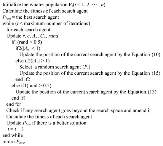
Figure 1.
Pseudo code of the WOA.
2.3. Improved Whale Optimization Algorithm
This section will introduce the improvement methods of the WOA, including population initialization based on tent map, mutation disturbance to the optimal individual and combination with differential evolution algorithms. Finally, the optimization performance of IMWOA is tested by several test functions and another five algorithms are used for comparison with IMWOA, including the ant lion algorithm (ALO), particle swarm optimization algorithm (PSO), moth to fire algorithm (MFO), multiverse algorithm (MVO) and WOA.
2.3.1. Tent Mapping Initialization
Initialization determines the distribution and the fitness of the initial population. The distribution of the initial population generated by random generation method, which is the default initialization method, is poor in the solution space. The initial population can achieve better spatial distribution when the tent mapping is applied for initialization. The individual position of the IMWOA is initialized by tent mapping in this study. The expression of the tent mapping is shown as follows [46].
is the chaotic map sequence generated, is the control parameter.
When , the obtained chaotic sequences have approximately uniform distribution density. So, the expression of the tent mapping is converted to Formula (17).
The steps to initialize the IMWOA population by tent mapping are as follows:
- (1)
- Generate randomly, which represents the initial values of chaotic variables, and make not equal to 0.5.
- (2)
- Generate the chaotic mapping sequence iteratively according to the method of Formula (17), and if the chaotic variable enters a cycle, proceed to step (4).
- (3)
- Judge the end condition. When the end condition is satisfied, proceed to step (5).
- (4)
- Disturb and regenerate chaotic sequences.
- (5)
- Map the obtained chaotic value into the solution space of the optimization problem to form the initial IMWOA population.
2.3.2. Variation Disturbance of Optimal Position
It can be seen from Formula (14) that the optimal individual is assumed to be the prey, which constantly affects the updating of other individuals in the population. This mechanism can bring many advantages to WOA. However, when the iteration number is small, this mechanism causes the WOA quickly enter the local search phase without finding enough excellent solutions, and makes the algorithm fall into local optimum. Therefore, adding nonlinear mutation disturbance to the optimal individual causes the optimal individual to change with a certain probability, so the ability of IMWOA to escape from the local optimal solution is enhanced. The expression of variation disturbance factor is shown in Formula (18).
is the current number of iterations, is the maximum number of iterations, is a random number in the range of [0,1]. The variation range of random disturbance also gradually decreases, which ensures that the local search accuracy of IMWOA will not be affected.
2.3.3. Differential Evolution Algorithm
The DE algorithm includes mutation, crossover and selection. New individuals are generated by mutation and crossover, and individuals with high fitness are retained by selection. Adding the DE to the IMWOA can further enhance the diversity of solutions and enhance the fitness of the IMWOA population.
- Mutation: Select one individual in the population as the current individual , and then select three individuals except randomly. First, two randomly selected individuals are subjected to a vector difference operation, and then the result is subjected to a vector sum operation with the third individual to generate a mutant individual. The Formula is shown as follows [47].is a new individual produced by mutation, , and are three randomly selected individuals, is a random number in the range of .
- Crossover: Crossover individual is composed of some elements of the current individual and mutation individual. The crossover Formula is shown in (20).is the j-th element of crossover individual. is the probability vector that controls the crossover. is used to generate dimensional random number vectors. is the control parameter to ensure the occurrence of crossover.
- Selection: Compare the fitness values of and , and retain the individuals with high fitness into the next generation population. The selection Formula is shown in (21).is the fitness value of .
The optimization process of IMWOA is as follows, and Figure 2 shows the flow chart of IMWOA.
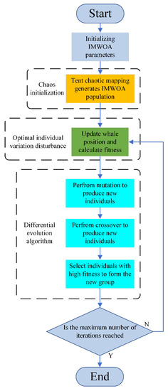
Figure 2.
IMWOA (improved whale algorithm) flow chart.
- (1)
- Initialize IMWOA parameters, including iteration number, solution dimension, population size, decision variable matrix size, cross probability, etc.
- (2)
- Generate the initial population of IMWOA based on the chaotic tent map, and calculate the fitness value.
- (3)
- Update the position and fitness of the whale population. The renewal process includes mutation disturbance to the optimal individual.
- (4)
- Carry the mutation and crossover operations of differential evolution algorithm to generate crossover individuals.
- (5)
- Select the individuals between the cross individuals and the original individuals according to the fitness to form the next generation.
- (6)
- Judge the end condition. If the end condition is met, output the optimal solution. Else, proceed to step (3).
2.4. IMWOA Performance Test
In this section, the IMWOA is tested by several test functions. The test function includes monotone function and non-monotone function, which can test the optimization performance of the IMWOA comprehensively. Table 1 shows the expressions of the test functions. The comparative experiments are made with several representative and widely used optimization algorithms, including MVO, PSO, MFO, ALO and WOA to show the performance of the IMWOA. Table 2 includes some special settings of algorithm parameters. Furthermore, the undeclared parameters are the default values. Table 3 shows the statistical test results, which are the average values for three sets of test results.

Table 1.
Test functions.

Table 2.
Special parameter setting table.

Table 3.
Statistical table of test results.
The test results are shown in Table 3, and all data less than 0.001 in the table are counted as 0. The optimization values of the IMWOA are obviously better than those of the other five algorithms. All the optimization values of the IMWOA are zero, but there are some errors in other algorithms, which shows that the IMWOA has excellent global search ability. The RMSE of the IMWOA is zero, which indicates that the optimization ability of the IMWOA is very stable. The IMWOA optimization value and RMSE are both better than the WOA, which proves that the improvement measures adopted can effectively enhance the optimization performance of the IMWOA. Moreover, for individual test functions (), the WOA has the problem of falling into local optimum, while the IMWOA avoids similar problems, which shows that the improved method can effectively enhance the performance of the IMWOA to escape from local optimal solution. In the same conditions, the IMWOA has the best optimization accuracy and stability, whether it has a monotone function or non-monotone function, which proves that the performance of IMWOA is excellent and that the improvement measures adopted in this study are reasonable and effective.
3. Input Data Preprocessing and Experimental Arrangement
Many meteorological factors have an impact on the PV power, and different meteorological factors have different effects on it. In this section, the Pearson coefficient is first applied to analyze the relationship between different meteorological factors and PV power. The meteorological factors strictly related to the PV output power are selected as the prediction input data. Then, wavelet denoising is used to denoise the input data to remove the noise in it, and the input data is normalized. Finally, the experimental arrangement is described.
3.1. Selection of Input Data
PV output power is closely related to meteorological factors including light intensity, ambient temperature, relative humidity, etc. Figure 3 shows the variation curve of the PV output power from 8 to 18 h in sunny and cloudy weather conditions. Sunny and cloudy weather are typical weather with representative characteristics, and the PV output power presents great differences in these two types of weather. In sunny weather, the changes of the meteorological factors are slow and the PV output power presents a regular parabola. In cloudy weather conditions, the meteorological factors have a greater fluctuation, resulting in PV output power also presenting a greater volatility, and the overall output power being low. Therefore, the external meteorological factors determine the PV power and they can be applied to accurately predict the PV power. Ignoring the key meteorological parameters will increase the prediction deviation. However, considering too many meteorological factors will greatly increase the workload of prediction, and excessive consideration of irrelevant factors will also reduce the prediction accuracy. So, accurately measuring the correlation between various meteorological factors and PV power and selecting the appropriate factors as the input data of the prediction model is important to enhance the prediction accuracy. The Pearson correlation coefficient is selected to measure the correlation between meteorological factors and PV output power. The expression of the Pearson coefficient is shown in (22).
and are variables with correlation. is the total number of data. In this problem, is the weather factor, is the output power of photovoltaic power generation, and is the correlation coefficient.
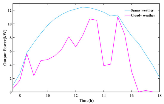
Figure 3.
Photovoltaic output power variation curve in different weather.
Table 4 shows the meaning of the Pearson coefficient. It indicates positive correlation when is greater than zero, it indicates no linear correlation when is equal to zero, and it indicates negative correlation when is less than zero.

Table 4.
Meaning of Pearson correlation coefficient
The correlation coefficients between PV power and the meteorological factors including light intensity, diffuse intensity, ambient temperature, wind speed and humidity are calculated. The test data are from a PV power station in Australia. Table 5 shows the calculation results of the correlation coefficient.

Table 5.
Correlation coefficient table of meteorological factors and photovoltaic power.
The correlation coefficient of wind speed and PV power remains at a low level, and the average correlation coefficient of six months is 0.321, showing a weak correlation. Moreover, the correlation coefficient fluctuates greatly among different months. The maximum correlation coefficient is 0.580, and the minimum correlation coefficient is −0.053, indicating that the correlation is extremely unstable. So, it is not suitable to select wind speed as the input data. The correlation coefficient of light intensity and PV power remains at a high value. The average correlation coefficient of six months is 0.993, the maximum and minimum correlation coefficient are 0.996 and 0.989, showing an extremely strong and stable correlation. So, it is appropriate to select the light intensity to predict the PV power. According to the same analysis method, the environmental temperature and humidity present stable moderate correlation with PV power, diffuse radiation and PV output power present stable weak correlation. In this study, the light intensity, ambient temperature and humidity are selected as input data considering the accuracy and complexity of the model.
3.2. Denoising and Normalization of Input Data
Light intensity, ambient temperature and relative humidity should be continuous and slowly changing signals, but, when affected by measurement conditions and other factors, these signals contain a lot of noise, which causes the measurement waveform to show the characteristics of fluctuation. The accuracy of the prediction model will be adversely affected if these data with noise are used for the training of the prediction model. So, it is necessary to take measures to reduce the noise in input data.
There are many data denoising methods, and many studies have also examined various data denoising methods [48], among which wavelet threshold denoising is widely used [49]. The signal containing noise is decomposed by wavelet. The decomposed signal has a larger signal wavelet coefficient and a smaller noise wavelet coefficient. Comparing the obtained wavelet coefficients with the threshold value, the wavelet coefficient that is higher than the threshold value is considered as the signal, and should be retained. Furthermore, the wavelet coefficient that is lower than the threshold value is considered as noise, and should be removed. Setting an appropriate threshold can achieve ideal denoising effect. Figure 4 shows the flow chart of wavelet threshold denoising, and the steps are shown below.
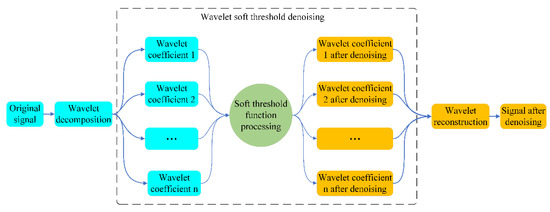
Figure 4.
Wavelet denoising flow chart.
- (1)
- Decompose the original signal and obtain the wavelet coefficients.
- (2)
- Set threshold and threshold function.
- (3)
- Denoise the wavelet coefficients by threshold to filter the noise information in the signal.
- (4)
- Reconstruct the processed wavelet coefficients to obtain the denoised signal.
The threshold denoising of wavelet denoising has a decisive impact on the denoising effect of the signal. Threshold denoising involves the selection of the threshold and threshold function. The selection of the threshold is complex and related to many aspects, and the default setting is generally used. There are two types of threshold functions. The first type is a hard threshold function, which sets the signal that is lower than the threshold to zero and keeps the signal that is higher than the threshold unchanged. The hard threshold function can cause the signal to retain more original information. However, the signal will break obviously near the threshold and the signal continuity is poor. The second type is a soft threshold function which processes the signal that is higher than the threshold by adding or subtracting the threshold value and sets the signal that is lower than the threshold to zero. The soft threshold function causes the denoised signal to become smoother and more continuous. Practice has proved that the prediction model trained by the signal processed by the soft threshold function has higher prediction accuracy. Therefore, this study applies the soft threshold function to preprocess the prediction input data. For intuitively reflecting the denoising effect of the soft threshold function, the data of daytime temperature, humidity and light intensity are intercepted for wavelet soft threshold denoising. Figure 5 shows the effect picture of wavelet soft threshold denoising.
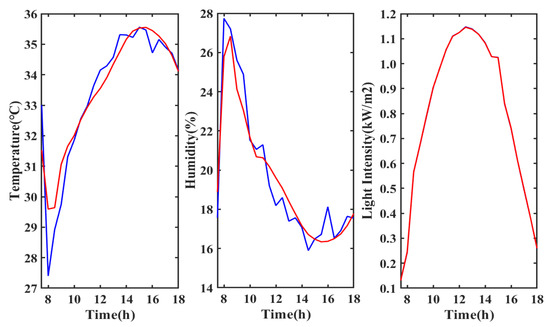
Figure 5.
Effect picture of wavelet soft threshold denoising.
The first picture is the temperature curve, the second one is the humidity curve, and the third one is the light intensity curve. The red line in Figure 5 represents the data denoised by wavelet soft threshold and the blue line is the original data. Since there are many noise signals in the original temperature and humidity data, the signal denoised by wavelet undergoes obvious changes compared to the original signal. However, the light intensity signal changes gently and contains less noise, so the signal after wavelet denoising undergoes no obvious change compared to the original signal. It can be found that the input signal without denoising contains high-frequency noise, and the signal waveform contains many turning points and fluctuates greatly. After wavelet soft threshold denoising, the waveform is smoother, many abrupt points are eliminated, and the real data are restored, which is beneficial for improving prediction accuracy. In this study, the training and testing input data are processed by wavelet soft threshold denoising to improve the prediction accuracy.
As shown in Figure 5, different meteorological factors have different units, and the variation range of the signals is also very different. So, they cannot be directly used for model training and prediction, and they need to be normalized. The normalization Formula is shown in Formula (23).
is the normalized data, is the non-normalized data, is the maximum value of the data, is the minimum value of the data.
In this study, the data of temperature, humidity, light intensity, PV power are normalized.
3.3. Experimental Arrangement
The prediction model of IMWOA-SVM was tested in sunny and cloudy weather conditions based on the data from Desert Knowledge Australia (DKA) Solar Center in Australia, and the prediction results were compared with five SVM models, and ELM and BP neural networks, respectively. Two days’ data of randomly selected typical weather are used for training, and one day’s randomly selected data are used for testing. The prediction period is from 8:00 to 18:00 in the daytime. Figure 6 shows the prediction flow chart of IMWOA-SVM, and the steps of using IMWOA-SVM to predict PV power are as follows.
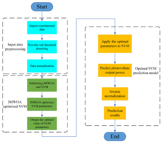
Figure 6.
Prediction flow chart of photovoltaic output power based on IMWOA-SVM.
- (1)
- Select training data and testing data in sunny and cloudy weather, respectively.
- (2)
- Preprocess training input data and testing input data by wavelet soft threshold denoising.
- (3)
- Normalize training and testing data.
- (4)
- Initialize the parameters of the IMWOA-SVM photovoltaic output power prediction model.
- (5)
- Train the prediction model by training data. Apply the IMWOA to optimize the SVM. Test the prediction model by the test data.
- (6)
- Obtain the optimal prediction model of PV power. Predict the PV power.
- (7)
- Normalize the prediction output power inversely and output the experimental results.
In the process of model optimization, the mean square error (MSE) of the prediction power and the actual power is used as the objective function of IMWOA optimization. The definition of MSE is shown in Formula (24).
is the predicted PV power, is the actual PV power, is the number of sample points.
Besides MSE, some other indexes are applied to evaluate the prediction results more comprehensively, including mean absolute error (MAE), root mean squared error (RMSE), R-square (R2) and mean absolute percentage error (MAPE). The definitions of these evaluation indexes are shown in Formula (25).
It should be noted that the larger is and the smaller the , , and are, the better the prediction results can track the actual output power.
4. Experimental Results and Discussion
In this section, the experiment results will be analyzed and discussed. The discussion is divided into two parts: the first part is the discussion of the experiment results in sunny weather, and the second part is the discussion of the experiment results in cloudy weather. In each weather condition, the IMWOA-SVM is first compared with other five models, including the ALO-SVM, MFO-SVM, MVO-SVM, PSO-SVM and WOA-SVM, and then compared with the BP neural network and ELM.
4.1. Prediction Results in Sunny Weather
4.1.1. Comparison with Other SVM Models
The IMWOA-SVM prediction model and the other five SVM models were tested with PV data of sunny weather and Figure 7 shows the test results.
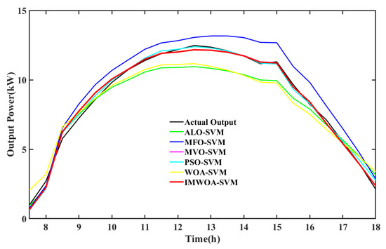
Figure 7.
Prediction results of SVM models in sunny weather.
The red line in Figure 7 represents the predicted power curve of IMWOA-SVM, the black line is the actual power curve, and other curves are shown in the legend. The PV power changes smoothly in sunny weather, showing a parabola type of high in the middle and low sections in both sides. The prediction results of the algorithm optimizing the SVM model can generally describe the trend of PV power. The prediction results of the ALO-SVM, MFO-SVM and WOA-SVM have some deviations with the actual power, and the prediction results of the IMWOA-SVM, MVO-SVM and PSO-SVM models are basically consistent with the actual power. In order to further intuitively show the difference of prediction accuracy, Figure 8 shows the accumulated value of absolute error of model prediction results in sunny weather.
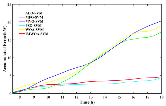
Figure 8.
Accumulated absolute error chart in sunny weather.
The accumulated absolute error gradually increases over the course of a day. The accuracy of ALO-SVM, MFO-SVM, WOA-SVM is poor, the accumulated error increases rapidly, and the accumulated error reaches more than 20 kW. The prediction accuracy of IMWOA-SVM, MVO-SVM, PSO-SVM is high. Although the accumulated error is also increasing, it has been kept at a low level and finally stabilized at 5 kW. The curve is relatively straight without an obvious mutation point, which shows that the prediction performance is stable. The accumulated absolute error of IMWOA-SVM is almost the same as that of MVO-SVM. The prediction accuracy of PSO-SVM is inferior to IMWOA-SVM in the first and final stages, and slightly better in the middle stage. The accumulated error values of the two models are roughly the same.
Figure 9 shows the statistical chart of the prediction error interval of the models in sunny weather. The transverse axis is the maximum value of the error range, and the longitudinal axis is the ratio of the prediction error in the corresponding error range. The more the bar graph is concentrated to the left, the more consistent the prediction result of corresponding model with the actual power curve, the more accurate the prediction is. Taking the IMWOA-SVM model as an example, the absolute error of IMWOA-SVM prediction results accounts for about 95% in the interval [0, 0.5] and about 5% in the interval [0.5, 1.0]. The absolute error of other models accounts for less than 95% in the interval of [0, 0.5], which shows that IMWOA-SVM has higher prediction accuracy.
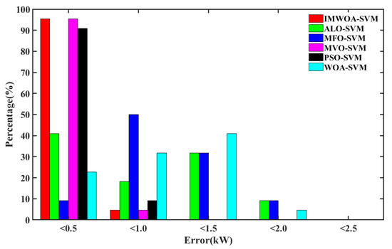
Figure 9.
Statistical chart of error interval in sunny weather.
4.1.2. Comparison with BP Neural Network and ELM
Figure 10 shows the prediction results of the IMWOA-SVM, BP neural network and ELM in sunny weather. The predicted results of the IMWOA-SVM fit the actual power curve best. The BP neural network can also predict the change of actual power well, but compared with the IMWOA-SVM, the error is obviously larger. The prediction results of ELM miss a lot of detailed information, and can hardly be applied in practice.
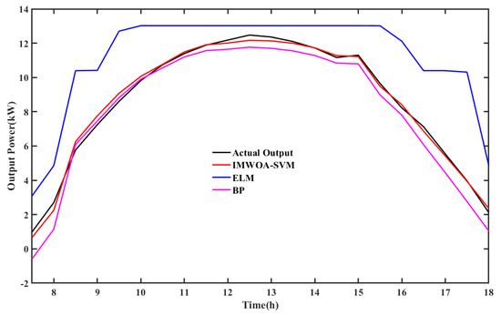
Figure 10.
Prediction results of BP and ELM in sunny weather.
The absolute error accumulation chart of BP and ELM is shown in Figure 11 to intuitively display the error. The accumulated error of the IMWOA-SVM prediction results increases slowly and the curve is relatively straight, which indicates that the IMWOA-SVM can maintain high accuracy throughout the whole period of time. However, the error curve of BP is gentle in the front section and warped in the tail section, which indicates that the accuracy of BP decreases at the tail end and the prediction performance is unstable. The accumulated error curve of ELM increases rapidly, and the front and back sections of the curve are obviously warped, which indicates that ELM prediction results are very unstable and the prediction accuracy is very poor.
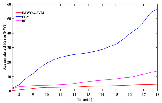
Figure 11.
Accumulated absolute error chart of BP and ELM in sunny weather.
Table 6 is the summary evaluation table of prediction results in sunny weather. Prediction results are comprehensively evaluated by MSE, RMSE, MAE, MAPE and R2. The bold font in the table indicates the optimal value of the evaluation index. The MSE of IMWOA-SVM is 0.069, RMSE is 0.263, MAPE is 0.047, R2 is 0.995, which reach the optimal value. The MAE is 0.212, which is 0.009 higher than that of PSO (0.203). Overall, the prediction result of IMWOA-SVM is the best.

Table 6.
Evaluation table of prediction results in sunny weather.
In conclusion, the prediction performance of the six SVM models, the BP neural network and the ELM is tested in this section based on the data of sunny weather. The test results prove that most of the SVM models are more accurate, while prediction accuracy of BP neural network and ELM is relatively poor. The reason is that BP neural network and ELM have a large demand for training data, while this study is based on small training samples. The training data consists of two days’ historical data, which is far from meeting the requirements of BP neural network and ELM for training data volume, so their prediction performance is poor. The SVM model has the advantage of less training data demand, so the overall prediction result is preferred, which is also the reason why SVM is selected for PV prediction in this study. Several evaluation indexes show that the prediction performance of IMWOA-SVM is the best.
4.2. Prediction Results in Cloudy Weather
In this section, we will test the PV prediction model in cloudy weather. The PV output power presents great volatility and instability in cloudy weather, which brings more difficulties to the prediction work. In such extreme conditions, the prediction performance of the prediction model can be tested more effectively.
4.2.1. Comparison with Other SVM Models
The prediction results of SVM models in cloudy weather is shown in Figure 12. In cloudy weather, the prediction deviations of ALO-SVM, MFO-SVM and WOA-SVM which perform poorly in sunny weather are still relatively large, and the prediction results of PSO-SVM and MVO-SVM with high accuracy also show obvious deviation and the prediction performance declines. Only the prediction result of the IMWOA-SVM proposed can track the actual output well. The absolute error accumulation chart of each model in cloudy weather is shown in Figure 13 to show the change of prediction error more intuitively.
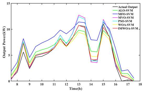
Figure 12.
Prediction results of SVM models in cloudy weather.
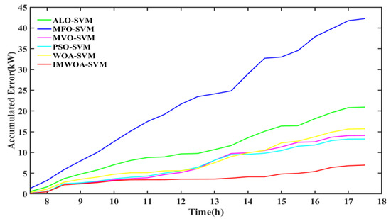
Figure 13.
Accumulated absolute error chart in cloudy weather.
In cloudy weather, the prediction error of prediction model generally increases due to the violent fluctuation of actual PV power. The PSO-SVM and MVO-SVM models with higher prediction accuracy in sunny weather have larger prediction error in cloudy weather, and the accumulated error increases to 15 KW, which shows that the performance of this two PV prediction model is not stable. It can achieve better prediction accuracy in sunny weather with small disturbances, but cannot achieve ideal prediction accuracy in cloudy weather with large disturbances. Although the prediction error of the IMWOA-SVM proposed also increases in cloudy weather, reaching about 7 KW, the rising range is not large and the IMWOA-SVM can still predict the changes of actual PV power. The accumulated error curve of the IMWOA-SVM is still relatively straight, which shows that the complex meteorological conditions of cloudy weather have little impact on the prediction performance of the IMWOA-SVM. It proves that the IMWOA-SVM has superior anti-interference ability and adaptability to different weather conditions.
Figure 14 shows the statistical chart of prediction error intervals in cloudy weather. The proportion of the IMWOA-SVM in the minimum error range is 90%, and the prediction accuracy is hardly affected. The prediction error of other models accounts for only 55% in the minimum range, and the prediction results of other models generally tend to the interval with larger error. The prediction errors become larger in complex weather, which is consistent with the previous conclusion. The results show that the IMWOA-SVM can achieve better prediction accuracy in both sunny and cloudy weather, which shows that the IMWOA-SVM has high prediction accuracy and better stability.
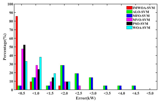
Figure 14.
Statistical chart of error interval in cloudy weather.
4.2.2. Comparison with BP Neural Network and ELM
In cloudy weather, the prediction accuracy of BP neural network is significantly reduced. The prediction curve of BP deviates from the actual curve, as shown in Figure 15. The deviation points are mainly concentrated in the actual power mutation, and only a few points can accurately describe the actual output power. The prediction result of ELM is still not ideal; the predicted curve deviates significantly from the actual curve, and lacks a significant amount of characteristic information on the actual power output curve.
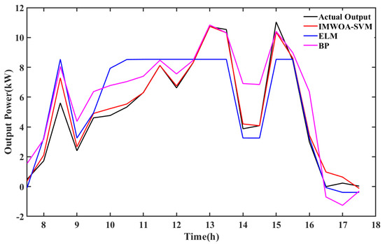
Figure 15.
Prediction results of BP and ELM in cloudy weather.
The accumulated absolute error chart of BP and ELM in cloudy weather is shown in Figure 16. The maximum accumulated error of BP is more than 25 kW in cloudy weather, while it is not more than 15 kw in sunny weather. The accumulated error curve of the BP neural network and ELM increases step by step. The curve up warping mainly occurs during the period when the actual power fluctuates greatly and, in the stable range of actual power, the accumulated error curve is relatively gentle. It proves that the data fluctuation has a great influence on the prediction accuracy of BP and ELM. The prediction performance is unstable, and the adaptability to weather types is poor.
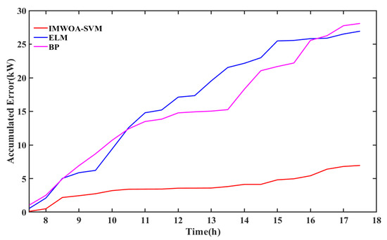
Figure 16.
Accumulated absolute error chart of BP and ELM in cloudy weather.
Finally, the comprehensive evaluation table of the model prediction results is given, as shown in Table 7. The MSE of the IMWOA-SVM is 0.257, the RMSE is 0.507, the MAE is 0.331, and the R2 is 0.979, all of which reach the optimal value. Due to the existence of zero value in cloudy weather data, the MAPE evaluation index is not used. The evaluation results of the IMWOA-SVM are better than other models in cloudy weather.

Table 7.
Evaluation table of prediction results in cloudy weather.
In conclusion, the prediction performance of the six SVM models, the BP neural network and the ELM has been tested, in this section, with the data of cloudy weather. The test results show that the accuracy of cloudy weather decreases compared with sunny weather. The prediction accuracy and stability of BP neural network and ELM are not better, and they are not suitable as the prediction model in this study. Other prediction models based on SVM have better prediction accuracy in sunny weather, but have poor prediction accuracy in cloudy weather, indicating that these models have poor adaptability and poor anti-interference ability. The proposed IMWOA-SVM model can achieve ideal prediction performance in both sunny and cloudy weather, especially in complex cloudy weather, and it can also achieve better prediction accuracy. The experimental results prove that the IMWOA-SVM model has better prediction accuracy and anti-interference ability, and prove that the proposed improvement measures in this study are effective.
5. Conclusions
PV output power has the characteristic of uncertainty, which is not conductive to the stability and security of power system. In different weather, PV power has significantly different characteristics, which increases the difficulty of power prediction. For further symmetrically improving the prediction accuracy of PV power in different weather conditions and promoting the use of clean energy, an improved whale algorithm optimizing SVM model is proposed in this study. The advantages of this model are that it can reduce the demand for input data, adapt to the changes of weather conditions, and achieve ideal prediction accuracy in complex weather conditions compared with similar prediction models. The research contents include the selection of input data, the preprocessing of data, the improvement of the optimization algorithm and the optimization of the SVM prediction model. The following conclusions are obtained.
- (1)
- The PV power is determined by some meteorological factors, and it has significantly different characteristics in different weather conditions. Through the correlation analysis, it is found that PV power has the strongest correlation with the meteorological factors including light intensity, ambient temperature and humidity. Furthermore, these meteorological factors can be used to accurately predict PV power.
- (2)
- The wavelet soft threshold denoising can be applied for the pretreatment of PV input data. It can effectively eliminate the noise contained in input data and improve the coherence of the input data, which is beneficial to remove the adverse impact of noise and enhance the stability of the prediction model in complex weather conditions.
- (3)
- The BP neural network and ELM have large demand for training data. When the training data are not sufficient, the ideal prediction accuracy cannot be achieved. SVM has less demand for training data, and can achieve ideal prediction accuracy when there is less training data, which is suitable for PV output power prediction models with less training data.
- (4)
- The optimization performance of WOA can be effectively improved through combination with the hybrid improved method. By combining the original WOA with tent chaos initialization, mutation disturbance of the optimal individual and DE algorithm, the comprehensive performance of the IMWOA is significantly enhanced.
- (5)
- The IMWOA-SVM photovoltaic output power prediction model applies wavelet denoising to process the predicted input data, and applies the hybrid improved whale algorithm to optimize the SVM, which significantly improves comprehensive prediction performance in different weather conditions.
- (6)
- The proposed IMWOA-SVM photovoltaic output power prediction model can symmetrically achieve the accurate prediction for PV power in different weather conditions, especially in complex weather conditions. It can provide the operation and scheduling department with reliable reference, help to improve the utilization rate of renewable energy power generation and maintain the security of renewable energy power systems. It is of great significance to the application of clean energy.
The input data selection method, input data preprocessing method, algorithm selection and improvement method and model optimization method proposed in this study constitute a complete prediction method of renewable energy generation output power. It can be applied not only to predict the PV power, but also to predict other similar renewable energy power. It provides a reference for the optimization and improvement of prediction models of other similar renewable energy and is expected to develop into a general method to predict the output power of renewable energy power.
This study has limitations. In the stage of selecting input data, the linear correlation between wind speed, temperature, humidity, light intensity, diffuse intensity and PV power is simply analyzed, but the complex nonlinear relationship behind the data is not deeply considered, which may cause some important data to be ignored. Future studies should enhance the optimization of the prediction method and the selection of input data to improve the performance of the IMWOA-SVM. In addition, this study is based on the SVM model; more types of models should be introduced into the prediction field to further improve the prediction accuracy in future research.
Author Contributions
Conceptualization, Y.-W.L. and H.F.; methodology, Y.-W.L. and H.F.; software H.-Y.L. and L.-L.L.; writing—original draft preparation, Y.-W.L., H.F., H.-Y.L. and L.-L.L. All authors have read and agreed to the published version of the manuscript.
Funding
This research was funded by the key project of the Tianjin Natural Science Foundation (Project No. 19JCZDJC32100) and the Natural Science Foundation of Hebei Province of China (Project No. E2018202282).
Institutional Review Board Statement
The study did not involve humans or animals.
Informed Consent Statement
The study did not involve humans or animals.
Data Availability Statement
Not Applicable.
Acknowledgments
This study was supported by the key project of the Tianjin Natural Science Foundation (Project No. 19JCZDJC32100) and the Natural Science Foundation of Hebei Province of China (Project No. E2018202282).
Conflicts of Interest
The authors declare no conflict of interest.
Notations
| Acronyms list | |
| ALO | Ant lion optimization algorithm |
| DE | Differential evolution algorithm |
| IMWOA | Improved whale optimization algorithm |
| MAPE | Mean absolute percent error |
| MFO | Moth to fire algorithm |
| MSE | Mean square error |
| PSO | Particle swarm optimization algorithm |
| RMSE | Root mean square error |
| SVM | Support vector machine |
| SVR | Support vector regression |
| WOA | Whale optimization algorithm |
| Nomenclature variables | |
| a, , u, | Iteration variables of whale algorithm |
| A, Cw | Iteration variables of whale algorithm |
| b | Spiral motion constant of whale or Regression bias |
| C | Penalty factor |
| C1, C2 | Learning factor |
| CR | Crossover probability |
| Maximum scale factor | |
| Maximum number of iterations | |
| Minimum scale factor | |
| t | Current iterations |
| U | New individuals obtained by crossing |
| X | Individual whale population |
| Optimal individual of whale population | |
| New individuals obtained by mutation | |
| Random individuals of whale population | |
| Current individuals | |
| Tent chaotic mapping sequence | |
| Nonlinear mapping function | |
| Permissible deviation | |
| Pearson correlation coefficient | |
| Relaxation variable | |
References
- Lin, P.; Peng, Z.; Lai, Y.; Cheng, S.; Chen, Z.; Wu, L. Short-term power prediction for photovoltaic power plants using a hybrid improved Kmeans-GRA-Elman model based on multivariate meteorological factors and historical power datasets. Energy Convers. Manag. 2018, 177, 704–717. [Google Scholar] [CrossRef]
- Li, Y.; Su, Y.; Shu, L. An ARMAX model for forecasting the power output of a grid connected photovoltaic system. Renew. Energy 2014, 66, 78–89. [Google Scholar] [CrossRef]
- Wang, H.; Yi, H.; Peng, J.; Wang, G.; Liu, Y.; Jiang, H.; Liu, W. Deterministic and probabilistic forecasting of photovoltaic power based on deep convolutional neural network. Energy Convers. Manag. 2017, 153, 409–422. [Google Scholar] [CrossRef]
- Chawda, G.S.; Mahela, O.P.; Gupta, N.; Khosravy, M.; Senjyu, T. Incremental Conductance Based Particle Swarm Optimization Algorithm for Global Maximum Power Tracking of Solar-PV under Nonuniform Operating Conditions. Appl. Sci. 2020, 10, 4575. [Google Scholar] [CrossRef]
- Bracale, A.; Carpinelli, G.; De Falco, P. A Probabilistic Competitive Ensemble Method for Short-Term Photovoltaic Power Forecasting. IEEE Trans. Sustain. Energy 2017, 8, 551–560. [Google Scholar] [CrossRef]
- Cheng, Z.; Liu, Q.; Zhang, W. Improved probability prediction method research for photovoltaic power output. Appl. Sci. 2019, 9, 2043. [Google Scholar] [CrossRef]
- Wang, J.; Li, P.; Ran, R.; Che, Y.; Zhou, Y. A short-term photovoltaic power prediction model based on the Gradient Boost Decision Tree. Appl. Sci. 2018, 8, 689. [Google Scholar] [CrossRef]
- Rodríguez, F.; Fleetwood, A.; Galarza, A.; Fontán, L. Predicting solar energy generation through artificial neural networks using weather forecasts for microgrid control. Renew. Energy 2018, 126, 855–864. [Google Scholar] [CrossRef]
- Zhang, J.; Tan, Z.; Wei, Y. An adaptive hybrid model for day-ahead photovoltaic output power prediction. J. Clean. Prod. 2020, 244, 118858. [Google Scholar] [CrossRef]
- El-Sehiemy, R.A.; Selim, F.; Bentouati, B.; Abido, M.A. A novel multi-objective hybrid particle swarm and salp optimization algorithm for technical economical environmental operation in power systems. Energy 2019, 193, 1084–1101. [Google Scholar] [CrossRef]
- Sanjari, M.J.; Gooi, H.B.; Nair, N.K.C. Power generation forecast of hybrid PV-Wind system. IEEE Trans. Sustain. Energy 2020, 11, 703–712. [Google Scholar] [CrossRef]
- Hossain, M.; Mekhilef, S.; Danesh, M.; Olatomiwa, L.; Shamshirband, S. Application of extreme learning machine for short term output power forecasting of three grid-connected PV systems. J. Clean. Prod. 2017, 167, 395–405. [Google Scholar] [CrossRef]
- Hu, Y.; Lian, W.; Han, Y.; Dai, S.; Zhu, H. A seasonal model using optimized multi-layer neural networks to forecast power output of pv plants. Energies 2018, 11, 326. [Google Scholar] [CrossRef]
- Wang, S.; Sun, Y.; Zhou, Y.; Mahfoud, R.J.; Hou, D. A new hybrid short-term interval forecasting of PV output power based on EEMD-SE-RVM. Energies 2019, 13, 87. [Google Scholar] [CrossRef]
- De Giorgi, M.G.; Congedo, P.M.; Malvoni, M. Photovoltaic power forecasting using statistical methods: Impact of weather data. IET Sci. Meas. Technol. 2014, 8, 90–97. [Google Scholar] [CrossRef]
- Reikard, G. Predicting solar radiation at high resolutions: A comparison of time series forecasts. Sol. Energy 2009, 83, 342–349. [Google Scholar] [CrossRef]
- Li, Y.; He, Y.; Su, Y.; Shu, L. Forecasting the daily power output of a grid-connected photovoltaic system based on multivariate adaptive regression splines. Appl. Energy 2016, 180, 392–401. [Google Scholar] [CrossRef]
- Liu, L.; Zhao, Y.; Chang, D.; Xie, J.; Ma, Z.; Sun, Q.; Yin, H.; Wennersten, R. Prediction of short-term PV power output and uncertainty analysis. Appl. Energy 2018, 228, 700–711. [Google Scholar] [CrossRef]
- Zhu, H.; Lian, W.; Lu, L.; Dai, S.; Hu, Y. An improved forecasting method for photovoltaic power based on adaptive BP neural network with a scrolling time window. Energies 2017, 10, 1542. [Google Scholar] [CrossRef]
- Priyadarshi, N.; Padmanaban, S.; Holm-Nielsen, J.B.; Blaabjerg, F.; Bhaskar, M.S. An Experimental Estimation of Hybrid ANFIS-PSO-Based MPPT for PV Grid Integration under Fluctuating Sun Irradiance. IEEE Syst. J. 2020, 14, 1218–1229. [Google Scholar] [CrossRef]
- Li, L.L.; Cheng, P.; Lin, H.C.; Dong, H. Short-term output power forecasting of photovoltaic systems based on the deep belief net. Adv. Mech. Eng. 2017, 9, 1–13. [Google Scholar] [CrossRef]
- Ni, Q.; Zhuang, S.; Sheng, H.; Wang, S.; Xiao, J. An optimized prediction intervals approach for short term PV power forecasting. Energies 2017, 10, 1669. [Google Scholar] [CrossRef]
- Wang, J.; Ran, R.; Zhou, Y. A short-term photovoltaic power prediction model based on an FOS-ELM algorithm. Appl. Sci. 2017, 7, 423. [Google Scholar] [CrossRef]
- Ni, Q.; Zhuang, S.; Sheng, H.; Kang, G.; Xiao, J.; Penrose, M. An ensemble prediction intervals approach for short-term PV power forecasting Improved differential evolution. Sol. Energy 2017, 155, 1072–1083. [Google Scholar] [CrossRef]
- Huang, C.M.T.; Huang, Y.C.; Huang, K.Y. A hybrid method for one-day ahead hourly forecasting of PV power output. In Proceedings of the 2014 9th IEEE Conference on Industrial Electronics and Applications, Hangzhou, China, 9–11 June 2014; Volume 5, pp. 526–531. [Google Scholar] [CrossRef]
- Bae, K.Y.; Jang, H.S.; Sung, D.K. Hourly Solar Irradiance Prediction Based on Support Vector Machine and Its Error Analysis. IEEE Trans. Power Syst. 2017, 32, 935–945. [Google Scholar] [CrossRef]
- Chen, P.; Yuan, L.; He, Y.; Luo, S. An improved SVM classi fi er based on double chains quantum genetic algorithm and its application in analogue circuit diagnosis. Neurocomputing 2016, 211, 202–211. [Google Scholar] [CrossRef]
- System, P.; Adaptive, U.; Dawan, P.; Sriprapha, K.; Kittisontirak, S.; Boonraksa, T. Comparison of Power Output Forecasting on the Photovoltaic System Using Adaptive Neuro-Fuzzy Inference Systems and Particle Swarm Optimization-Artificial Neural Network Model. Energies 2020, 13, 351. [Google Scholar] [CrossRef]
- Dai, S.; Niu, D.; Han, Y. Forecasting of power grid investment in China based on support vector machine optimized by differential evolution algorithm and greywolf optimization algorithm. Appl. Sci. 2018, 8, 636. [Google Scholar] [CrossRef]
- Eseye, A.T.; Zhang, J.; Zheng, D. Short-term photovoltaic solar power forecasting using a hybrid Wavelet-PSO-SVM model based on SCADA and Meteorological information. Renew. Energy 2018, 118, 357–367. [Google Scholar] [CrossRef]
- Lin, K.P.; Pai, P.F. Solar power output forecasting using evolutionary seasonal decomposition least-square support vector regression. J. Clean. Prod. 2016, 134, 456–462. [Google Scholar] [CrossRef]
- Shang, C.; Wei, P. Enhanced support vector regression based forecast engine to predict solar power output. Renew. Energy 2018, 127, 269–283. [Google Scholar] [CrossRef]
- Lin, G.Q.; Li, L.L.; Tseng, M.L.; Liu, H.M.; Yuan, D.D.; Tan, R.R. An improved moth-flame optimization algorithm for support vector machine prediction of photovoltaic power generation. J. Clean. Prod. 2020, 253, 119966. [Google Scholar] [CrossRef]
- VanDeventer, W.; Jamei, E.; Thirunavukkarasu, G.S.; Seyedmahmoudian, M.; Soon, T.K.; Horan, B.; Mekhilef, S.; Stojcevski, A. Short-term PV power forecasting using hybrid GASVM technique. Renew. Energy 2019, 140, 367–379. [Google Scholar] [CrossRef]
- Ebrahimgol, H.; Aghaie, M.; Zolfaghari, A.; Naserbegi, A. A novel approach in exergy optimization of a WWER1000 nuclear power plant using whale optimization algorithm. Ann. Nucl. Energy 2020, 145, 107540. [Google Scholar] [CrossRef]
- Chen, H.; Yang, C.; Heidari, A.A.; Zhao, X. An efficient double adaptive random spare reinforced whale optimization algorithm. Expert Syst. Appl. 2020, 154, 113018. [Google Scholar] [CrossRef]
- Sun, W.Z.; Wang, J.S.; Wei, X. An improved whale optimization algorithm based on different searching paths and perceptual disturbance. Symmetry 2018, 10, 210. [Google Scholar] [CrossRef]
- Yuan, X.; Miao, Z.; Liu, Z.; Yan, Z.; Zhou, F. Multi-strategy ensemble whale optimization algorithm and its application to analog circuits intelligent fault diagnosis. Appl. Sci. 2020, 10, 3667. [Google Scholar] [CrossRef]
- Mohammadi, B.; Mehdizadeh, S. Modeling daily reference evapotranspiration via a novel approach based on support vector regression coupled with whale optimization algorithm. Agric. Water Manag. 2020, 237, 106145. [Google Scholar] [CrossRef]
- Tsoupos, A.; Khadkikar, V. A Novel SVM Technique with Enhanced Output Voltage Quality for Indirect Matrix Converters. IEEE Trans. Ind. Electron. 2019, 66, 832–841. [Google Scholar] [CrossRef]
- Mirjalili, S.; Lewis, A. The Whale Optimization Algorithm. Adv. Eng. Softw. 2016, 95, 51–67. [Google Scholar] [CrossRef]
- Bai, L.; Han, Z.; Ren, J.; Qin, X. Research on feature selection for rotating machinery based on Supervision Kernel Entropy Component Analysis with Whale Optimization Algorithm. Appl. Soft. Comput. 2020, 92, 106245. [Google Scholar] [CrossRef]
- Gao, Y.; Chen, K.; Gao, H.; Zheng, H.; Wang, L.; Xiao, P. Energy Consumption Prediction for 3-RRR PPM through Combining LSTM Neural Network with Whale Optimization Algorithm. Math. Probl. Eng. 2020, 2020, 1–17. [Google Scholar] [CrossRef]
- Strumberger, I.; Bacanin, N.; Tuba, M.; Tuba, E. Resource scheduling in cloud computing based on a hybridized whale optimization algorithm. Appl. Sci. 2019, 9, 4893. [Google Scholar] [CrossRef]
- Li, L.; Liu, Y.; Tseng, M.; Lin, G. Reducing environmental pollution and fuel consumption using optimization algorithm to develop combined cooling heating and power system operation strategies. J. Clean. Prod. 2020, 247, 119082. [Google Scholar] [CrossRef]
- Song, Y.; Chen, Z.; Yuan, Z. New Chaotic PSO-Based Neural Network Predictive Control for Nonlinear Process. IEEE Trans. Neural Netw. 2007, 18, 595–601. [Google Scholar] [CrossRef] [PubMed]
- Das, S.; Suganthan, P.N. Differential Evolution: A Survey of the State-of-the-Art. IEEE Trans. Evol. Comput. 2011, 15, 4–31. [Google Scholar] [CrossRef]
- Alickovic, E.; Kevric, J.; Subasi, A. Performance evaluation of empirical mode decomposition, discrete wavelet transform, and wavelet packed decomposition for automated epileptic seizure detection and prediction. Biomed. Signal Process. Control. 2018, 39, 94–102. [Google Scholar] [CrossRef]
- Fu, J.; Cai, F.; Guo, Y.; Liu, H.; Niu, W. An Improved VMD-Based Denoising Method for Time Domain Load Signal Combining Wavelet with Singular Spectrum Analysis. Math. Probl. Eng. 2020, 2020, 1–14. [Google Scholar] [CrossRef]
Publisher’s Note: MDPI stays neutral with regard to jurisdictional claims in published maps and institutional affiliations. |
© 2021 by the authors. Licensee MDPI, Basel, Switzerland. This article is an open access article distributed under the terms and conditions of the Creative Commons Attribution (CC BY) license (http://creativecommons.org/licenses/by/4.0/).