Generalizing Local Density for Density-Based Clustering

Abstract

Discovering densely-populated regions in a dataset of data points is an essential task for density-based clustering. To do so, it is often necessary to calculate each data point’s local density in the dataset. Various definitions for the local density have been proposed in the literature. These definitions can be divided into two categories: Radius-based and k Nearest Neighbors-based. In this study, we find the commonality between these two types of definitions and propose a canonical form for the local density. With the canonical form, the pros and cons of the existing definitions can be better explored, and new definitions for the local density can be derived and investigated.

1. Introduction

Density-based clustering is the task of detecting densely-populated regions (called clusters) separated by sparsely-populated or empty regions in a data set of data points. It is an unsupervised process that can discover clusters of arbitrary shapes [1]. Many density-based clustering algorithms have been proposed in the literature [2,3,4,5,6,7,8,9], but most of them adopt their definitions of local density. Since clusters are derived based on each data point’s local density, using an inappropriate definition for local density could yield bad clustering results. Thus, it is crucial to define local density properly for density-based clustering.

This study divides the definitions for local density in the literature into two categories: Radius-based and k Nearest Neighbors-based (or kNN-based for short). Radius-based local density uses a radius to specify the neighborhood of a data point, and the data points within a data point’s neighborhood mainly determine the local density of the data point. In contrast, kNN-based local density uses the k nearest neighbors or the reverse k nearest neighbors of a data point to derive its local density.

In this study, we propose a canonical form for local density. All previous definitions for local density can be viewed as a special case of the canonical form. The canonical form decomposes local density definition into three parts: The contribution set, contribution function, and integration operator. The contribution set of a data point specifies the set of data points that contribute to the data point’s local density. The contribution function calculates the contribution of a data point to the local density of another data point. The integration operator is used to combine the contributions of the data points in the contribution set to yield local density.

The advantage of using this canonical form is twofold. First, it allows us to interpret the implicit difference between different definitions for local density. For example, in Section 2.2, we show that the kNN-based local density defined in [6,7] implicitly uses a radius equal to one and $\sqrt{k}$, respectively. Second, this canonical form facilitates exploring the pros and cons of these existing definitions for local density. We can then combine these definitions’ merits to derive suitable definitions for local density for the problem at hand.

The rest of this paper is organized as follows. Section 2 reviews the existing definitions for local density. Section 3 proposes the canonical form for local density and shows how these definitions fit the canonical form. Section 4 describes how to derive new definitions for local density using this canonical form. Section 5 conducts an experiment to show how the three parts (i.e., contribution set, contribution function, and integration operator) of the canonical form affect local density distribution. Section 6 concludes this paper.

2. Review on Local Density

Most density-based clustering algorithms require calculating each data point’s local density to derive clusters in the dataset. However, there is no standard definition for a data point’s local density. Many definitions for local density have been proposed in the literature. Based on the parameters used in the definitions, we can divide the existing definitions into two categories. A radius-based definition uses a parameter $ϵ$ for the radius of a data point’s neighborhood, and a kNN-based definition uses a parameter k to limit the scope of the data points involved to the k nearest neighbors. In this section, we review these two types of definitions. For ease of exposition, some notations are defined in Table 1.

Table 1. Notations.

$X=\left\{x_1,\cdots ,x_n\right\}$	the dataset of n data points to be clustered
$\mathsf{\rho }\left(x_i\right)$	the local density of a data point $x_i\in X$
$\mathrm{d}\left(x_i,x_j\right)$	the distance between two data points $x_i$ and $x_j$
$ϵ$	the radius of a data point’s neighborhood
${ϵ}_p$	the radius derived from top p% of all pairs’ distances. (1st used in Section 4)
${ϵ}_k$	the radius derived using the parameter k and Equation (8). (1st used in Section 4)
${ϵ}_{kP}$	the radius derived using the P-th percentile of the distances between all data points and their k-th nearest neighbors. (1st used in Section 4)
$N_k\left(x_i\right)$	the set of $k$ nearest neighbors of $x_i$. (1st used in Equation (4))
$R_k\left(x_i\right)$	the set of reverse $k$ nearest neighbors of $x_i$. (1st used in Equation (12))
$y_i^j$	the j-th nearest neighbor of $x_i$. (1st used in Section 2.2)
${\delta }_i^j$	the distance between $x_i$ and its j-th nearest neighbor $y_i^j$. (1st used in Equation (8))
$C_i$	the set of data points that contribute to the density of $x_i$. (1st used in Equation (17))
$c\left(x_i,x_j\right)$	the contribution of $x_j$ to the density of $x_i$. (1st used in Equation (17))

2.1. Radius-Based Local Density

As described earlier, a radius-based local density uses parameter $ϵ$ to specify the radius of a data point’s neighborhood. Consider a dataset $X=\left\{x_1,x_2,\cdots ,x_n\right\}$ of n data points and the local density $\mathsf{\rho }\left(x_i\right)$ of a data point $x_i\in X$. A radius-based local density ensures that those data points within $x_i$’s neighborhood have a large contribution to $\mathsf{\rho }\left(x_i\right)$ and that the data points outside $x_i$’s neighborhood have little or no contribution to $\mathsf{\rho }\left(x_i\right)$. In what follows, we describe two definitions for the radius-based local density in the literature.

In [4], the local density of a data point is defined as the number of data points within the data point’s neighborhood, which is given as follows:

$$\mathsf{\rho }\left(x_i\right)={{\displaystyle \sum }}_{x_j\in X}X\left(\frac{\mathrm{d}\left(x_i,x_j\right)}{ϵ}\right)$$

(1)

where

$$X\left(d\right)=\{\begin{array}{cc}1& \mathrm{if} d<1\\ 0& \mathrm{otherwise}\end{array}$$

(2)

and $\mathrm{d}\left(x_i,x_j\right)$ is the distance between data points $x_i$ and $x_j$. Thus, each data point $x_j\in X$ with $\mathrm{d}\left(x_i,x_j\right)<ϵ$ contributes 1 to $\mathsf{\rho }\left(x_i\right)$. In [2], the constraint $\mathrm{d}\left(x_i,x_j\right)\le ϵ$ is adopted instead of $\mathrm{d}\left(x_i,x_j\right)<ϵ$, i.e., each data point $x_j\in X$ with $\mathrm{d}\left(x_i,x_j\right)\le ϵ$ contributes 1 to $\mathsf{\rho }\left(x_i\right)$. However, this change should not make a significant difference on $\mathsf{\rho }\left(x_i\right)$.

Instead of using the radius $ϵ$ as a hard threshold in Equation (1), [4] proposed a local density definition that uses an exponential kernel, as shown in Equation (3).

$$\mathsf{\rho }\left(x_i\right)={{\displaystyle \sum }}_{x_j\in X}{e}^{-{\left(\frac{\mathrm{d}\left(x_i,x_j\right)}{ϵ}\right)}^2}$$

(3)

With Equation (3), each data point $x_j\in X$ contributes $e^{-{\left(\frac{\mathrm{d}\left(x_i,x_j\right)}{ϵ}\right)}^2}$ to $\mathsf{\rho }\left(x_i\right)$. Notably, $e^{-{\left(\frac{\mathrm{d}\left(x_i,x_j\right)}{ϵ}\right)}^2}$ is an inverse S-shaped function of $\frac{\mathrm{d}\left(x_i,x_j\right)}{ϵ}$ with an inflection point at $\frac{\mathrm{d}\left(x_i,x_j\right)}{ϵ}=\frac{1}{\sqrt{2}}$. That is, the value of $e^{-{\left(\frac{\mathrm{d}\left(x_i,x_j\right)}{ϵ}\right)}^2}$ decreases at an increasing speed as $\frac{\mathrm{d}\left(x_i,x_j\right)}{ϵ}$ approaches $\frac{1}{\sqrt{2}}$ from 0, and then at a decreasing speed after $\frac{\mathrm{d}\left(x_i,x_j\right)}{ϵ}$ is greater than $\frac{1}{\sqrt{2}}$. Thus, to be exact, Equation (3) uses a soft threshold at $\mathrm{d}\left(x_i,x_j\right)=\frac{ϵ}{\sqrt{2}}$, instead of at $\mathrm{d}\left(x_i,x_j\right)=ϵ$. Figure 1 shows the curves of $e^{-{\left(\frac{\mathrm{d}\left(x_i,x_j\right)}{ϵ}\right)}^2}$ and its first and secondary derivatives with respect to $\frac{\mathrm{d}\left(x_i,x_j\right)}{ϵ}$. The three black dots indicate that the inflection point occurs when the first and secondary derivatives reach minimum and zero, respectively.

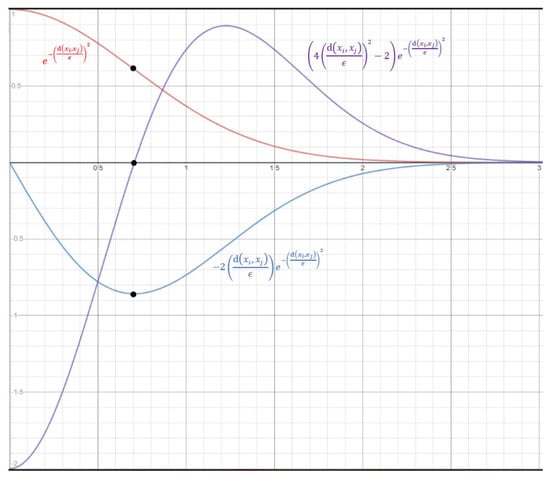
Figure 1. The horizontal axis is $\frac{\mathrm{d}\left(x_i,x_j\right)}{ϵ}$ and the vertical axis is the values of $e^{-{\left(\frac{\mathrm{d}\left(x_i,x_j\right)}{ϵ}\right)}^2}$ (in red) and its first (in blue) and secondary (in purple) derivatives with respect to $\frac{\mathrm{d}\left(x_i,x_j\right)}{ϵ}$.

The proper value for $ϵ$ is dataset-dependent. Thus, instead of setting the value for $ϵ$ directly, Ref. [4] used another parameter, p, to derive $ϵ$. Specifically, $ϵ$ is set to the top p% distance of all pairs’ distances in $X$, and 1 ≤ p ≤ 2 is recommended. Alternatively, Ref. [5] used parameter k to determine the value of $ϵ$.

2.2. kNN-Based Local Density

Although the radius-based local density is intuitive and straightforward, using the same radius for all data points may be inappropriate for some datasets. The kNN-based local density adopts a different approach by restricting only the k nearest neighbors contributing to the local density. In what follows, we describe four definitions of the kNN-based local density in the literature.

In [6], a data point’s local density is defined using an exponential kernel and the distances to k nearest neighbors, as shown in Equation (4).

$$\mathsf{\rho }\left(x_i\right)={{\displaystyle \sum }}_{x_j\in N_k\left(x_i\right)}{e}^{-\mathrm{d}\left(x_i,x_j\right)}$$

(4)

where $N_k\left(x_i\right)$ denotes the set of k nearest neighbors of $x_i$. Notably, $e^{-\mathrm{d}\left(x_i,x_j\right)}$ is a monotonically decreasing function of $\mathrm{d}\left(x_i,x_j\right)$. Its derivative to $\mathrm{d}\left(x_i,x_j\right)$ is $-e^{-\mathrm{d}\left(x_i,x_j\right)}$, which is a monotonically increasing function of $\mathrm{d}\left(x_i,x_j\right)$. As $\mathrm{d}\left(x_i,x_j\right)$ increases from 0, the value of $e^{-\mathrm{d}\left(x_i,x_j\right)}$ drops at an exponentially decreasing speed. Such a property may cause a significantly different effect for different datasets. For example, if the maximum distance between any $x_i\in X$ and $x_j\in N_k\left(x_i\right)$ is small, then a fixed change to $\mathrm{d}\left(x_i,x_j\right)$ will cause a large change to $e^{-\mathrm{d}\left(x_i,x_j\right)}$. In contrast, if the minimum distance between any $x_i\in X$ and $x_j\in N_k\left(x_i\right)$ is large, then a fixed change to $\mathrm{d}\left(x_i,x_j\right)$ will only cause a small change to $e^{-\mathrm{d}\left(x_i,x_j\right)}$. The cause of such an inconsistent behavior is because Equation (4) is not unit-less. Alternatively, the function $e^{-\mathrm{d}\left(x_i,x_j\right)}$ can be interpreted as a unit-less function $e^{-\left(\frac{\mathrm{d}\left(x_i,x_j\right)}{ϵ}\right)}$ with a fixed radius $ϵ=1$ for any dataset.

Reference [7] used the mean of $x_i$’s squared distance to its k nearest neighbors to derive $\mathsf{\rho }\left(x_i\right)$, as shown in Equation (5):

$$\mathsf{\rho }\left(x_i\right)=e^{-\frac{1}{k}{\displaystyle \sum }_{x_j\in N_k\left(x_i\right)}{\left(\mathrm{d}\left(x_i,x_j\right)\right)}^2}$$

(5)

Similar to Equation (4), $\mathsf{\rho }\left(x_i\right)$ in Equation (5) is a monotonically decreasing function of $\frac{1}{k}{\displaystyle \sum }_{x_j\in N_k\left(x_i\right)}{\left(\mathrm{d}\left(x_i,x_j\right)\right)}^2$ and is not unit-less. We can rewrite Equation (5) to remove the summation in the exponent as follows.

$$\mathsf{\rho }\left(x_i\right)=e^{-{{\displaystyle \sum }}_{x_j\in N_k\left(x_i\right)}{\left(\frac{\mathrm{d}\left(x_i,x_j\right)}{\sqrt{k}}\right)}^2}={{\displaystyle \prod }}_{x_j\in N_k\left(x_i\right)}{e}^{-{\left(\frac{\mathrm{d}\left(x_i,x_j\right)}{\sqrt{k}}\right)}^2}$$

(6)

Similar to $e^{-{\left(\frac{\mathrm{d}\left(x_i,x_j\right)}{ϵ}\right)}^2}$ in Equation (3), $e^{-{\left(\frac{\mathrm{d}\left(x_i,x_j\right)}{\sqrt{k}}\right)}^2}$ in Equation (6) is an inverse S-shaped function of $\frac{\mathrm{d}\left(x_i,x_j\right)}{\sqrt{k}}$ with an inflection point at $\frac{\mathrm{d}\left(x_i,x_j\right)}{\sqrt{k}}=\frac{1}{\sqrt{2}}$. The function $e^{-{\left(\frac{\mathrm{d}\left(x_i,x_j\right)}{\sqrt{k}}\right)}^2}$ can also be interpreted as a unit-less function $e^{-{\left(\frac{\mathrm{d}\left(x_i,x_j\right)}{ϵ}\right)}^2}$ with a fixed radius $ϵ=\sqrt{k}$ for any dataset. That is, Equation (6) uses the parameter k to implicitly derive the radius $ϵ$, which controls the positions of the inflection point of the inverse S-shaped function $e^{-{\left(\frac{\mathrm{d}\left(x_i,x_j\right)}{\sqrt{k}}\right)}^2}$.

Reference [5] proposed a kNN-based unit-less definition for $\mathsf{\rho }\left(x_i\right)$, which is similar to Equation (3) but limits the data points contributing to $\mathsf{\rho }\left(x_i\right)$ only to $N_k\left(x_i\right)$, as shown in Equation (7).

$$\mathsf{\rho }\left(x_i\right)={{\displaystyle \sum }}_{x_j\in N_k\left(x_i\right)}{e}^{-{\left(\frac{\mathrm{d}\left(x_i,x_j\right)}{ϵ}\right)}^2}$$

(7)

Reference [5] also used the parameter k to determine the value of $ϵ$ as follows:

$$ϵ={\mu }^k+\sqrt{\frac{1}{\left|X\right|-1}{{\displaystyle \sum }}_{x_i\in X}{\left({\delta }_i^k-{\mu }^k\right)}^2}$$

(8)

$${\mu }^k=\frac{1}{\left|X\right|}{\displaystyle \sum }_{x_i\in X}{\delta }_i^k$$

(9)

where ${\delta }_i^k$ is the distance between $x_i$ and its kth nearest neighbor, and ${\mu }^k$ is the mean of ${\delta }_i^k$ of all data points in $X$. Equation (8) derives $ϵ$ as ${\mu }^k$ plus the standard deviation of ${\delta }_i^k$, and thus a larger k yields a larger $ϵ$.

Reference [8] used the distance between $x_i$ and the mean of its k nearest neighbors to derive $\mathsf{\rho }\left(x_i\right)$, as follows:

$$\mathsf{\rho }\left(x_i\right)=e^{-{\left(\mathrm{d}\left(x_i,{\overline{x}}_i\right)\right)}^2}$$

(10)

$${\overline{x}}_i=\frac{1}{k}{\displaystyle \sum }_{x_j\in N_k\left(x_i\right)}^{}{x}_j$$

(11)

This definition could yield counterintuitive results because using the mean of k nearest neighbors sacrifices their distribution. For example, consider the case of two nearest neighbors $y_i^1$ and $y_i^2$ of $x_i$ located at opposite sides of $x_i$, and $\mathrm{d}\left(x_i,y_i^1\right)=\mathrm{d}\left(x_i,y_i^2\right)$. Then, $\mathsf{\rho }\left(x_i\right)$ remains unchanged independent of the values of $\mathrm{d}\left(x_i,y_i^1\right)$ and $\mathrm{d}\left(x_i,y_i^2\right)$, which contradicts the intuition that larger $\mathrm{d}\left(x_i,y_i^1\right)$ and $\mathrm{d}\left(x_i,y_i^2\right)$ should result in smaller $\mathsf{\rho }\left(x_i\right)$.

Reference [8] also proposed using the number of reverse $k$ nearest neighbors as the local density, as follows:

$$\mathsf{\rho }\left(x_i\right)=\left|R_k\left(x_i\right)\right|$$

(12)

where $R_k\left(x_i\right)=\{x_j\in X|x_i\in N_k\left(x_j\right)\}$ is the set of reverse $k$ nearest neighbors of $x_i$. This definition could render a data point $x_i$ having $\mathsf{\rho }\left(x_i\right)=0$ even though $x_i$ is in a densely-populated region. Thus, this definition should be used with caution.

To avoid the bias of $k$ nearest neighbors, [10] proposed the using mutual $k$ nearest neighbors to define local density, as follows:

$$SNN\left(x_i,x_j\right)=\left(N_k\left(x_i\right){{\displaystyle \cup }}^{ }\left\{x_i\right\}\right){{\displaystyle \cap }}^{ }\left(N_k\left(x_j\right){{\displaystyle \cup }}^{ }\left\{x_j\right\}\right)$$

(13)

$$Sim\left(x_i,x_j\right)=\{\begin{array}{cc}\frac{{\left|SNN\left(x_i,x_j\right)\right|}^2}{{{\displaystyle \sum }}_{x_p\in SNN\left(x_i,x_j\right)}\left(\mathrm{d}\left(x_i,x_p\right)+\mathrm{d}\left(x_j,x_p\right)\right)}& if x_i,x_j\in SNN\left(x_i,x_j\right)\\ 0,& otherwise\end{array}$$

(14)

$$\mathsf{\rho }\left(x_i\right)={\displaystyle \sum }_{x_j\in L\left(x_i\right)}Sim\left(x_i,x_j\right)$$

(15)

where $SNN\left(x_i,x_j\right)$ is the set of mutual $k$ nearest neighbors of $x_i$ and $x_j$; $Sim\left(x_i,x_j\right)$ is the similarity between $x_i$ and $x_j$; and $L\left(x_i\right)$ is the set of k data points chosen from $X\backslash \left\{x_i\right\}$ with the largest $Sim\left(x_i,x_j\right)$.

3. Canonical Form for Local Density

In this section, we first propose the canonical form for local density. Then, we show how the existing definitions for local density fit the canonical form.

3.1. Canoncial Form

Based on the review in Section 2, this section proposes a canonical form for local density. Consider dataset $X$ and data point $x_i\in X$. The canonical form for the local density $\mathsf{\rho }\left(x_i\right)$ includes three parts: The contribution set $C_i$, the contribution function $c\left(x_i,x_j\right)$, and the integration operator. The contribution set $C_i\subset X$ is the set of data points contributing to $\mathsf{\rho }\left(x_i\right)$. Three possible values for $C_i$ are commonly used in the literature: $N_k\left(x_i\right)$, $X$, and $B_{ϵ}\left(x_i\right)=\{x_j\in X|\mathrm{d}\left(x_i,x_j\right)<ϵ\}$. The first value $N_k\left(x_i\right)$ is the set of $k$ nearest neighbors of $x_i$, where $k$ is the parameter [5,6,7]. The second value$X$ is the entire dataset [4]. The third value $B_{ϵ}\left(x_i\right)$ uses $ϵ$ to specify the radius of a data point’s neighborhood, and only the data points within the neighborhood of $x_i$ contribute to $\mathsf{\rho }\left(x_i\right)$ [2,4].

The contribution function $c\left(x_i,x_j\right)$ calculates the contribution of a data point $x_j\in C_i$ to the density of $x_i$. A general form for $c\left(x_i,x_j\right)$ is proposed as follows:

$$c\left(x_i,x_j\right)=e^{-{\left(\frac{\mathrm{d}\left(x_i,x_j\right)}{ϵ}\right)}^m}$$

(16)

where $ϵ$ is the radius of a data point’s neighborhood. In the literature, the value of the exponent $m$ is 1, 2, or $\infty$. In practice, we can use any m ≥ 1 to achieve a different effect, which is discussed further in Section 4.

The integration operator integrates the contributions of the data points in $C_i$ to yield $\mathsf{\rho }\left(x_i\right)$. In the literature, either the summation $\mathsf{\Sigma }$ or the product $\mathsf{\Pi }$ operator is used. Thus, the canonical form for local density can be defined using Equation (17) or Equation (18), as follows:

$$\mathsf{\rho }\left(x_i\right)={\displaystyle \sum }_{x_j\in C_i}c\left(x_i,x_j\right)$$

(17)

$$\mathsf{\rho }\left(x_i\right)={\displaystyle \prod }_{x_j\in C_i}c\left(x_i,x_j\right)$$

(18)

3.2. Fit the Existing Definitions to the Canoncial Form

Based on the canonical form defined in Section 3.1, we can derive most of the definitions for local density reviewed in Section 2, and Table 2 summarizes the results. We have excluded the definition in Equation (10) because it tends to conflict with the basic property of local density, as described in Section 2.

Table 2. Equations (3), (4), (6), (7) and (19)–(21) fit the canonical forms defined in Equations (16)–(18).

Equation	$\Pi$ or $\Sigma$	$C_i$	$c\left(x_i,x_j\right)$	m	$ϵ$
(19) ${\displaystyle \sum }_{x_j\in X}{e}^{-{\left(\frac{\mathrm{d}\left(x_i,x_j\right)}{ϵ}\right)}^{\infty }}$	$\mathsf{\Sigma }$	$X$	$e^{-{\left(\frac{\mathrm{d}\left(x_i,x_j\right)}{ϵ}\right)}^{\infty }}$	$\infty$	$ϵ$ is set to the distance at the top p% of all pairs’ distances in $X$, where p is a parameter [4].
(3) ${\displaystyle \sum }_{x_j\in X}{e}^{-{\left(\frac{\mathrm{d}\left(x_i,x_j\right)}{ϵ}\right)}^2}$	$\mathsf{\Sigma }$	$X$	$e^{-{\left(\frac{\mathrm{d}\left(x_i,x_j\right)}{ϵ}\right)}^2}$	2	$ϵ$ is set to the distance at the top p% of all pairs’ distances in $X$, where p is a parameter [4].
(4) ${\displaystyle \sum }_{x_j\in N_k\left(x_i\right)}{e}^{-\left(\frac{\mathrm{d}\left(x_i,x_j\right)}{1}\right)}$	$\mathsf{\Sigma }$	$N_k\left(x_i\right)$	$e^{-\left(\frac{\mathrm{d}\left(x_i,x_j\right)}{1}\right)}$	1	1
(6) ${\displaystyle \prod }_{x_j\in N_k\left(x_i\right)}{e}^{-{\left(\frac{\mathrm{d}\left(x_i,x_j\right)}{\sqrt{k}}\right)}^2}$	$\mathsf{\Pi }$	$N_k\left(x_i\right)$	$e^{-{\left(\frac{\mathrm{d}\left(x_i,x_j\right)}{\sqrt{k}}\right)}^2}$	2	$\sqrt{k}$
(7) ${\displaystyle \sum }_{x_j\in N_k\left(x_i\right)}{e}^{-{\left(\frac{\mathrm{d}\left(x_i,x_j\right)}{ϵ}\right)}^2}$	$\mathsf{\Sigma }$	$N_k\left(x_i\right)$	$e^{-{\left(\frac{\mathrm{d}\left(x_i,x_j\right)}{ϵ}\right)}^2}$	2	$ϵ$ is derived from the distance between each data point to its kth nearest neighbor using Equation (8) [5].
(20) ${\displaystyle \sum }_{x_j\in R_k\left(x_i\right)}1$	$\mathsf{\Sigma }$	$R_k\left(x_i\right)$	1
(21) ${\displaystyle \sum }_{x_j\in L\left(x_i\right)}Sim\left(x_i,x_j\right)$	$\mathsf{\Sigma }$	$N_k\left(x_i\right){{\displaystyle \cap }}^{ }{R}_k\left(x_i\right)$	$Sim\left(x_i,x_j\right)$

Notably, we have transformed Equation (1) to Equation (19) below such that it can match the canonical form in Equation (17):

$$\mathsf{\rho }\left(x_i\right)={{\displaystyle \sum }}_{x_j\in X}{e}^{-{\left(\frac{\mathrm{d}\left(x_i,x_j\right)}{ϵ}\right)}^{\infty }},$$

(19)

Here, $e^{-{\left(\frac{\mathrm{d}\left(x_i,x_j\right)}{ϵ}\right)}^{\infty }}$ = 1 if $0<\frac{\mathrm{d}\left(x_i,x_j\right)}{ϵ}<1$, and $e^{-{\left(\frac{\mathrm{d}\left(x_i,x_j\right)}{ϵ}\right)}^{\infty }}$ = 0 if $\frac{\mathrm{d}\left(x_i,x_j\right)}{ϵ}>1$. Thus, Equations (1) and (19) yield exactly the same results except at $\frac{\mathrm{d}\left(x_i,x_j\right)}{ϵ}=1$ where Equation (1) has $c\left(x_i,x_j\right)=0$, but Equation (19) has $c\left(x_i,x_j\right)=e^{-1}$.

Similarly, we have transformed Equation (12) to Equation (20) below such that it can match the canonical form in Equation (17).

$$\mathsf{\rho }\left(x_i\right)={{\displaystyle \sum }}_{x_j\in R_k\left(x_i\right)}1$$

(20)

Additionally, Equation (15) is rewritten as Equation (21) to avoid using $L\left(x_i\right)$.

$$\mathsf{\rho }\left(x_i\right)={\displaystyle \sum }_{x_j\in N_k\left(x_i\right){{\displaystyle \cap }}^{ }{R}_k\left(x_i\right)}Sim\left(x_i,x_j\right)$$

(21)

Notably, by (14), $Sim\left(x_i,x_j\right)\ne 0$ only if $x_i,x_j\in SNN\left(x_i,x_j\right)$, and by (13), $SNN\left(x_i,x_j\right)\backslash \left\{x_i\right\}\subseteq N_k\left(x_i\right)$ contains at most k data points, and thus we replace $L\left(x_i\right)$ in (15) by $N_k\left(x_i\right){{\displaystyle \cap }}^{ }{R}_k\left(x_i\right)$ or simply $N_k\left(x_i\right)$ to speed up the computation.

By fitting the existing definitions to the canonical form, we can see that most of them use a radius $ϵ$, explicitly or implicitly. With Table 2, we can better explore the pros and cons of these definitions. For example, Equation (4) uses a fixed radius of $ϵ=1$, and Equation (6) uses radius $ϵ=\sqrt{k}$ which only depends on the parameter k. Both of them do not consider the data points’ distribution in the dataset to determine $ϵ$. Consequently, the chosen value for $ϵ$ may not be adaptable to different datasets. In contrast, Equations (3), (7) and (19) not only use a parameter (p or k) but also consider the distribution of the data points to decide a proper value for $ϵ$.

4. Derive New Definitions Using the Canonical Form

As described in Section 3.1, there are three parts in the canonical form for local density. We can combine possible values for the three parts from the existing definitions to form new definitions for local density. However, some combinations may generate undesirable results, e.g., replacing the contribution set $N_k$ in Equation (6) with $X$. Thus, it is crucial to understand how the possible values for the three parts affect the results.

First, consider the integration operator in the canonical form. As shown in the second column of Table 2, most of the existing definitions for local density used the summation operator $\mathsf{\Sigma }$. We can replace the summation operator $\mathsf{\Sigma }$ with the product operator $\mathsf{\Pi }$ (or vice versa) to yield new definitions for local density. The operators $\mathsf{\Pi }$ and $\mathsf{\Sigma }$ affect the local density differently. For example, if the value of ${\displaystyle \sum }_{x_j\in C_i}c\left(x_i,x_j\right)$ is fixed, then the more evenly distributed the value of $c\left(x_i,x_j\right)$ for all $x_j\in C_i$, the larger the value of ${\displaystyle \prod }_{x_j\in C_i}c\left(x_i,x_j\right)$. On the contrary, if the value of ${\displaystyle \prod }_{x_j\in C_i}c\left(x_i,x_j\right)$ is fixed, then the more unevenly distributed the value of $c\left(x_i,x_j\right)$ for all $x_j\in C_i$, the larger the value of ${\displaystyle \sum }_{x_j\in C_i}c\left(x_i,x_j\right)$. Notably, the contribution $c\left(x_i,x_j\right)$ grows as the distance $\mathrm{d}\left(x_i,x_j\right)$ decreases. If we intend to give higher local density to those data points with more evenly distributed distances to their respective neighbors in $C_i$, then the product operator $\mathsf{\Pi }$ is adopted. Otherwise, the summation operator $\mathsf{\Sigma }$ should be used in most cases.

Next, consider the contribution function $c\left(x_i,x_j\right)$. The general form of $c\left(x_i,x_j\right)$, defined in Equation (16), contains two parameters: The exponent m and the radius $ϵ$. First, focus on the impact of using different values for m. We can view $e^{-{\left(\frac{\mathrm{d}\left(x_i,x_j\right)}{ϵ}\right)}^m}$ in Equation (16) as a function of $\frac{\mathrm{d}\left(x_i,x_j\right)}{ϵ}$. Figure 2 shows that the value of m affects the shape of the function curve. For m > 1, $e^{-{\left(\frac{\mathrm{d}\left(x_i,x_j\right)}{ϵ}\right)}^m}$ is an inverse S-shaped function of $\frac{\mathrm{d}\left(x_i,x_j\right)}{ϵ}$ with an inflection point at $\frac{\mathrm{d}\left(x_i,x_j\right)}{ϵ}=\sqrt[m]{\frac{m-1}{m}}$. As the value of m approaches infinity, the inflection point approaches $\frac{\mathrm{d}\left(x_i,x_j\right)}{ϵ}=1$, yielding $e^{-{\left(\frac{\mathrm{d}\left(x_i,x_j\right)}{ϵ}\right)}^m}=e^{-1}$, and the function $e^{-{\left(\frac{\mathrm{d}\left(x_i,x_j\right)}{ϵ}\right)}^m}$ approximates the step function in Equation (2). Notably, if m = 1, $e^{-{\left(\frac{\mathrm{d}\left(x_i,x_j\right)}{ϵ}\right)}^m}$ is not an inverse S-shaped function. The function curves for m = 1, 1.5, 2, 3, 4, and 50 are shown in Figure 2, where the positions of the inflection points are indicated with solid circles. To choose a suitable value for m, we can check whether the problem at hand prefers that a small increase in $\mathrm{d}\left(x_i,x_j\right)$ does not cause too much decrease in $c\left(x_i,x_j\right)$ when $\mathrm{d}\left(x_i,x_j\right)<$ $ϵ$. If this is the case, then a large value for m should be adopted to move the inflection point to the right, i.e., closer to $\frac{\mathrm{d}\left(x_i,x_j\right)}{ϵ}=1$.

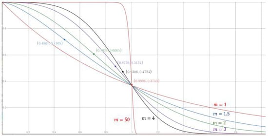
Figure 2. The contribution $c\left(x_i,x_j\right)$ for different values of m. The horizontal axis is $\frac{\mathrm{d}\left(x_i,x_j\right)}{ϵ}$, and the vertical axis is the contribution $c\left(x_i,x_j\right)=e^{-{\left(\frac{\mathrm{d}\left(x_i,x_j\right)}{ϵ}\right)}^m}$, as defined in Equation (16).

Next, consider the radius $ϵ$ of a data point’s neighborhood. The value of $ϵ$ should be dataset-dependent. For example, in [4], $ϵ$ is set to the distance at the top p% of all pairs’ distances in $X$, where p is a parameter. This method’s intuition is to have ⌊p(n − 1)/200⌋ data points within a data point’s neighborhood on average. However, this method tends to emphasize the dense regions and overlooks the sparse regions in the dataset. We denote the radius derived using this method by ${ϵ}_p$. In [5], $ϵ$ is set to the mean plus one standard deviation of all data points’ distances to their respective k-th nearest neighbors (see Equation (8)). This method is sensitive to the outliers in the dataset and the value of k. We denote the radius derived using this method by ${ϵ}_k$.

To avoid the shortcomings of the above two methods, we integrate both methods and propose a new method, shown in Algorithm 1. The new method requires two parameters: k and P. First, it collects the distance of each data point to its k-th nearest neighbor. Then, it sorts these distances in ascending order and sets $ϵ$ to the P-th percentile location, i.e., the $\lceil \frac{P\times n}{100}\rceil$-th distance, where n is the number of data points in the dataset. This new method considers each data point’s k-th nearest neighbor instead of the top p% of all pairs’ distances. Thus, it is less likely to overlook the sparse regions in the dataset. Furthermore, because the new method does not use mean and standard deviation, it is less sensitive to outliers than the second method. We denote the radius derived using this method by ${ϵ}_{kP}$.

Algorithm 1: The proposed method to derive ϵ.

Input: the set of data points $X\in {ℝ}_{n\times m}, k, \mathrm{and} P$ Output: the radius $ϵ$ 1. Set $S=\left\{{\delta }_i^k\right| x_i\in X\}$, where ${\delta }_i^k$ is the distance between $x_i$ and its k-th nearest neighbor. 2. Sort the elements in $S$ in ascending order. 3. Set $s = \lceil \frac{P\times n}{100}\rceil .$ 4. Set $ϵ=$ the s-th element in S. 5. Return $ϵ$

Finally, consider the contribution set $C_i$. As described in Section 3.1, $N_k\left(x_i\right)$, $X$, and $B_{ϵ}\left(x_i\right)$ are three commonly used values for $C_i$. Setting $C_i=X$ allows every data point contributing to $\mathsf{\rho }\left(x_i\right).$ It should only be used when the adopted $c\left(x_i,x_j\right)$ is near zero for any data point $x_j$ far from $x_i$ (e.g., Equation (16) with a large m value). For a data point $x_i$ in a dense region, its k nearest neighbors are likely to locate within its neighborhood, i.e., $B_{ϵ}\left(x_i\right)\supset N_k\left(x_i\right)$. However, for $x_i$ in a sparse region, $B_{ϵ}\left(x_i\right)\subset N_k\left(x_i\right)$ usually holds.

Using the product operator $\mathsf{\Pi }$ with $C_i=X$ (i.e., $\mathsf{\rho }\left(x_i\right)={\displaystyle \prod }_{x_j\in X}c\left(x_i,x_j\right)$) is a poor combination. Most of the data points in $X$ are far from $x_i$ thus, this combination involves multiplying many small $c\left(x_i,x_j\right)$ rendering a small $\mathsf{\rho }\left(x_i\right)$ that fails to represent the local density of $x_i$ properly. In contrast, using the summation operator $\mathsf{\Sigma }$ with $C_i=X$ does not cause such a problem.

Using the product operator $\mathsf{\Pi }$ with $C_i=B_{ϵ}\left(x_i\right)$ could also render strange results. For example, let $h$ be the current local density of $x_i$, and $y\notin X$ be a data point where $\mathrm{d}\left(x_i,y\right)$ is less than the distance between $x_i$ and $x_i$’s nearest neighbor in $X$. Intuitively, adding $y$ to $X$ should increase the local density of $x_i$. However, according to Equation (16), $c\left(x_i,x_j\right)$ is between 0 and 1 for any two data points $x_i$ and $x_j$. Thus, with the addition of $y$ to $X$, the local density of $x_i$ becomes $h\ast c\left(x_i,y\right)$, which is less than the original local density $h$. Thus, the combination of using the product operator $\mathsf{\Pi }$ and $C_i=B_{ϵ}\left(x_i\right)$ is also a poor definition for local density.

5. Experiment

5.1. Experiment Design

For brevity, we use a tuple with four components to describe a definition for local density, where the first component indicates the integration operator, the second component indicates the contribution set, and the third and the fourth components indicate the exponent $m$ and the radius $ϵ$ in the contribution function, respectively. For example, the row for Equation (7) in Table 2 can be represented as $\left(\mathsf{\Sigma }, N_k,2,{ϵ}_k\right)$. This representation facilitates modifying an existing definition to create new definitions. For example, $\left(\mathsf{\Pi }, N_k,2,{ϵ}_k\right)$, $\left(\mathsf{\Sigma }, N_k,20,{ϵ}_k\right),$ and $\left(\mathsf{\Sigma }, N_k,2,{ϵ}_{kP}\right)$ are three new definitions modified from $\left(\mathsf{\Sigma }, N_k,2,{ϵ}_k\right)$.

This experiment is divided into four tests. In each test, we use the definition $\left(\mathsf{\Sigma }, N_k,2,{ϵ}_k\right)$ proposed in [5] as the benchmark and vary one component in the tuple to study how this component affects the results. In Test 1, we compare three different ways (i.e., ${ϵ}_p$, ${ϵ}_k$, and ${ϵ}_{kP}$, described in Section 4) to derive radius $ϵ$. Here, ${ϵ}_p$ and ${ϵ}_{kP}$ are derived by setting the parameters p = 2 and P = 75, respectively. Parameter k is also set to 5 to 50 in a step of 5 for both ${ϵ}_{kP}$ and ${ϵ}_k$. Test 2 compares the three definitions $\left(\mathsf{\Sigma }, N_k,2,{ϵ}_k\right)$, $\left(\mathsf{\Sigma }, X,2,{ϵ}_k\right)$, and $\left(\mathsf{\Sigma }, B_{ϵ}\left(x_i\right),2,{ϵ}_k\right)$ to study the impact of using different values for the contribution set $C_i$. Test 3 compares the three definitions $\left(\mathsf{\Sigma }, N_k,2,{ϵ}_k\right)$,$\left(\mathsf{\Sigma }, N_k,4,{ϵ}_k\right)$, and $\left(\mathsf{\Sigma }, N_k,8,{ϵ}_k\right)$ to study the impact of using different values for the exponent $m$. Test 4 compares the two definitions $\left(\mathsf{\Sigma }, N_k,2,{ϵ}_k\right)$ and $\left(\mathsf{\Pi }, N_k,2,{ϵ}_k\right)$ to study the impact of using a different integration operator. In Tests 2 to 4, parameter k is set to 10 to derive ${ϵ}_k$ and $N_k$.

This experiment uses 16 well-known two-dimensional synthetic datasets. Table 3 shows the number of points and the number of clusters in these datasets.

Table 3. Number of points and number of clusters in the 16 synthetic datasets.

Dataset	Number of Clusters	Number of Points
Spiral [11]	3	312
Flame [12]	2	240
Aggregation [13]	7	788
Jain [14]	2	373
D31 [15]	31	3100
R15 [15]	15	600
Compound [16]	6	399
A1 [17]	20	3000
A2 [17]	35	5250
A3 [17]	50	7500
S1 [18]	15	5000
S2 [18]	15	5000
S3 [18]	15	5000
S4 [18]	15	5000
Path_based [11]	3	300
Unbalance [19]	8	6500

5.2. Test 1: Comparing the Radiuses ${ϵ}_p$, ${ϵ}_k$, and ${ϵ}_{kP}$

Test 1 compares radiuses ${ϵ}_p$, ${ϵ}_k$, and ${ϵ}_{kP}$ derived by the three methods described in Section 4. Obviously, increasing the values of p and P increases the values for ${ϵ}_p$ and ${ϵ}_{kP}$, respectively.

Figure 3 shows the experimental results of ${ϵ}_p$, ${ϵ}_k$, and ${ϵ}_{kP}$ by setting p = 2, P = 75, and k = 5 to 50 in a step of 5. The larger the value of k, the larger the values of ${ϵ}_k$ and ${ϵ}_{kP}$. In most cases, ${ϵ}_k>{ϵ}_{kP}$. For smaller datasets, ${ϵ}_p$ tends to be smaller than ${ϵ}_k$ and ${ϵ}_{kP}$. It appears that the size of the dataset influences the behaviors of ${ϵ}_p$, ${ϵ}_k$, and ${ϵ}_{kP}$ differently. Let n denote the size of the dataset $X$. The number of possible pairs of the data points in $X$ is $\frac{n\left(n-1\right)}{2}$. Since ${ϵ}_p$ is set to the $\lfloor \frac{n\left(n-1\right)}{2}\times \frac{p}{100}\rfloor$-th smallest value of all pairs’ distances in $X$, the location of ${ϵ}_p$ is linear with $n^2$. In contrast, ${ϵ}_{kP}$ is set to the $\lfloor n\times \frac{P}{100}\rfloor$-th smallest value of the distances between all data points and their k-th nearest neighbors. That is, the location of ${ϵ}_{kP}$ is only linear with n. Thus, the dataset size appears to have a greater impact on ${ϵ}_p$ than on ${ϵ}_{kP}$.

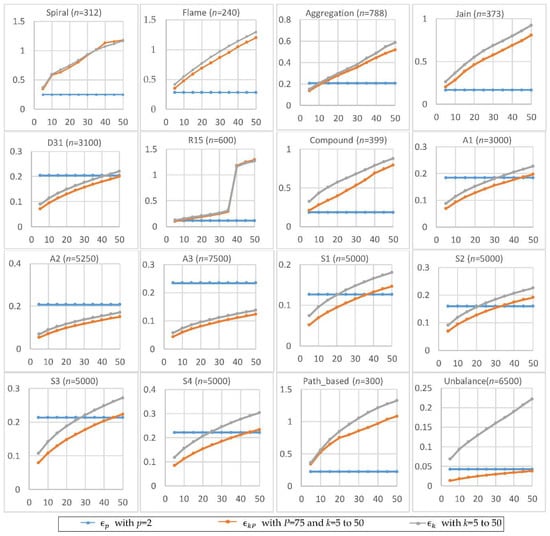
Figure 3. The radiuses ${ϵ}_p$, ${ϵ}_k$, and ${ϵ}_{kP}$ for p = 2, P = 75, and k = 5 to 50. The horizontal axis is the value of k, and the vertical axis is the value of radius.

Two small datasets (Compound dataset and Path_based dataset) and two large datasets (D31 dataset and A2 dataset) are selected to show the impact of the database size on ${ϵ}_p$, ${ϵ}_k$, and ${ϵ}_{kP}$. Three definitions, $\left(\mathsf{\Sigma }, N_k,2,{ϵ}_k\right)$, $\left(\mathsf{\Sigma }, N_k,2,{ϵ}_p\right)$, and $\left(\mathsf{\Sigma }, N_k,2,{ϵ}_{kP}\right)$, are used to calculate each data point’s local density, where the values of ${ϵ}_p$, ${ϵ}_k$, and ${ϵ}_{kP}$ (shown in Table 4) are derived by setting parameters p = 2, P = 75, and k =10. Notably, $\left(\mathsf{\Sigma }, N_k,2,{ϵ}_k\right)$ is the definition proposed in [5].

Table 4. ${ϵ}_p$ (p = 2), ${ϵ}_k$ (k = 10), and ${ϵ}_{kP}$ (k = 10 and P = 75) for four datasets.

Dataset	Compound	Path_Based	D31	A2
${ϵ}_p$	0.182606	0.223688	0.203595	0.206687
${ϵ}_{kP}$	0.280839	0.522962	0.094954	0.071405
${ϵ}_k$	0.430744	0.558793	0.114488	0.088676

In Figure 4, the color scale legend on each subfigure’s right indicates the measure of local density. For the two small datasets (i.e., Compound and Path_based), we have ${ϵ}_p<{ϵ}_{kP}<{ϵ}_k$, and thus using $ϵ={ϵ}_k$ or ${ϵ}_{kP}$ results in more data points having high local density than using $ϵ={ϵ}_p$ does, as shown in the upper two rows of Figure 4. In contrast, for the two large datasets (i.e., D31 and A2), ${ϵ}_p>{ϵ}_k>{ϵ}_{kP}$, and thus using $ϵ={ϵ}_p$ results in more data points having high local density than using $ϵ={ϵ}_k$ or ${ϵ}_{kP}$, as shown in the lower two rows of Figure 4.

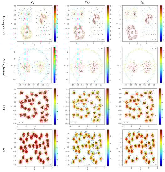
Figure 4. The local densities calculated using ${ϵ}_p$, ${ϵ}_k$, or ${ϵ}_{kP}$ for the data points in four datasets (i.e., Path_based, Compound, D31, and A2). The horizontal and the vertical coordination show the position of data points, and the color indicates the value of local densities.

5.3. Test 2: Impact of the Contribution Set $C_i$ on Local Density

Test 2 adopts three definitions, $\left(\mathsf{\Sigma }, N_k,2,{ϵ}_k\right)$, $\left(\mathsf{\Sigma }, X,2,{ϵ}_k\right)$, and $\left(\mathsf{\Sigma }, B_{ϵ}\left(x_i\right),2,{ϵ}_k\right)$, to calculate local density and evaluates the impact of using different values for $C_i$. Here, $k$ is set to 10 to derive ${ϵ}_k$ and $N_k$. The results are shown in Figure 5, where the subfigures in the same row are the results for a dataset and the subfigures in the same column are the results using the same method to determine $C_i$.

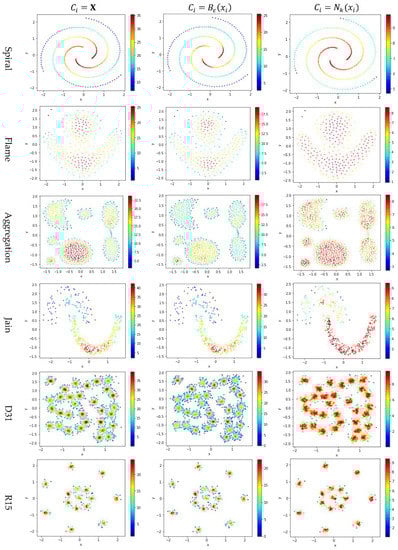
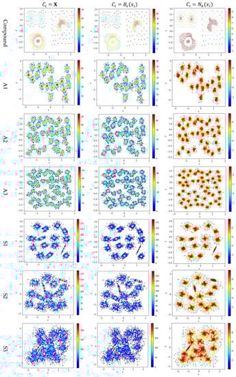
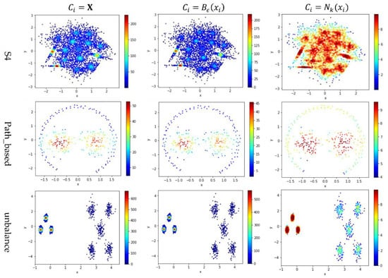
Figure 5. The local densities calculated using $C_i=X$, $B_{ϵ}\left(x_i\right)$, or $N_k\left(x_i\right)$. The horizontal and the vertical coordination show the position of data points, and the color indicates the value of local densities.

In Figure 5, the color scale legend on each subfigure’s right indicates the measure of local density. A large local density range is usually preferred because it provides more discrepancy to compare the local density among data points. Using $C_i=X$ has the largest local density range than using $C_i=B_{ϵ}\left(x_i\right)$ or $C_i=N_k\left(x_i\right)$ because using $C_i=X$ combines all data points’ contributions and Test 2 adopts the summation operator. Using $C_i=N_k\left(x_i\right)$ results in a much smaller range of local density than using $C_i=B_{ϵ}\left(x_i\right)$ does, indicating that, for any data point $x_i$ in a densely-populated region, $B_{ϵ}\left(x_i\right)\supset N_k\left(x_i\right)$ usually holds.

In the literature, all kNN-based methods (e.g., Equations (4), (6), and (7) in Table 2) adopted $C_i=N_k\left(x_i\right)$ to calculate the local density. Figure 5 shows that replacing $C_i=N_k\left(x_i\right)$ with $C_i=B_{ϵ}\left(x_i\right)$ or $C_i=X$ can enlarge the range of local density. Using $C_i=N_k\left(x_i\right)$ tends to result in more data points within the high-density regions (see the subfigures in column 3 of Figure 5). For example, the subfigure of “Flame” database using $C_i=N_k\left(x_i\right)$ shows that a majority of the data points have high local densities, making it difficult to partition the two densely-populated regions in the dataset. It is better to have each densely-populated region surrounded by low-density data points to facilitate clustering, e.g., the subfigure for “aggregation” dataset using $C_i=B_{ϵ}\left(x_i\right)$. Therefore, overall, using $C_i=B_{ϵ}\left(x_i\right)$ is preferred.

However, for datasets containing both high-density clusters and low-density clusters (e.g., the Path_based dataset and the Unbalance dataset in the last two rows of Figure 5), using $C_i=N_k\left(x_i\right)$ or $C_i=B_{ϵ}\left(x_i\right)$ tends to yield very low local density for the data points in the low-density clusters. A dense-based clustering algorithm must handle this situation carefully to avoid omitting the low-density clusters.

5.4. Test 3: Impact of the Exponent m on Local Density

Test 3 varies the value of $m$ in the contribution function $c\left(x_i,x_j\right)=e^{-{\left(\frac{\mathrm{d}\left(x_i,x_j\right)}{ϵ}\right)}^m}$ to study the impact of $m$ on the local density. Specifically, we compare three definitions, $\left(\mathsf{\Sigma }, N_k,2,{ϵ}_k\right)$,$\left(\mathsf{\Sigma }, N_k,4,{ϵ}_k\right)$, and $\left(\mathsf{\Sigma }, N_k,8,{ϵ}_k\right)$, where $k$ is set to 10 to derive ${ϵ}_k$ and $N_k$. The results are shown in Figure 6, where the subfigures in the same row are the results for a dataset, and the subfigures in the same column are the results using the same value for $m$.

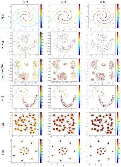
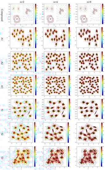
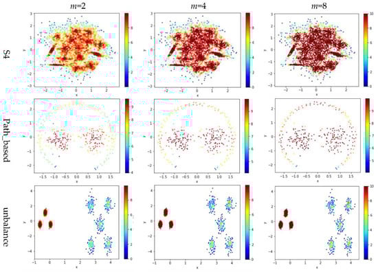
Figure 6. The local densities calculated using m = 2, 4, or 10 in $c\left(x_i,x_j\right)$. The horizontal and the vertical coordination show the position of data points, and the color indicates the value of local densities.

Comparing the subfigures in the same row of Figure 6 reflects that a larger m incurs more data points to have a higher local density. For those datasets with nicely separated clusters (e.g., dataset R15), using a large m helps identify the cores of the clusters. However, for datasets with poorly separated clusters (e.g., dataset S4), using a large m makes it challenging to spot the boundary between two adjacent clusters. For datasets containing both high-density clusters and low-density clusters (e.g., the Unbalance dataset), the impact of the value of m on the local density is not significant.

5.5. Test 4: Impact of the Integration Operator ($\Pi$ or $\Sigma$) on Local Density

Test 4 studies the impact of using different integration operator ($\mathsf{\Pi }$ or $\mathsf{\Sigma }$) using two definitions $\left(\mathsf{\Sigma }, N_k,2,{ϵ}_k\right)$ and $\left(\mathsf{\Pi }, N_k,2,{ϵ}_k\right)$, to calculate local density. As in Tests 2 and 3, $k$ is set to 10 to derive ${ϵ}_k$ and $N_k$. The results are shown in Figure 7, where the subfigures in the same column are the results using the same integration operator.

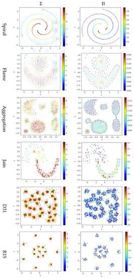
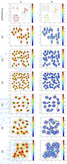
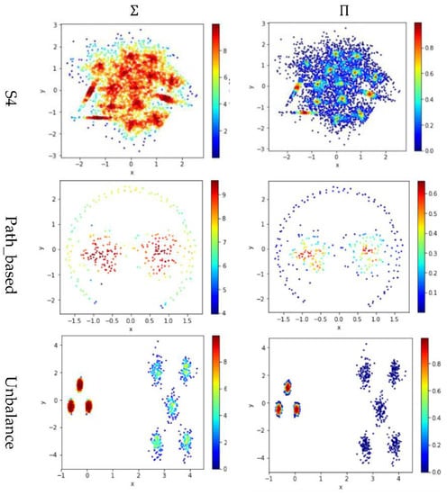
Figure 7. The local densities calculated using different integration operator ($\mathsf{\Pi }$ or $\mathsf{\Sigma }$). The horizontal and the vertical coordination show the position of data points, and the color indicates the value of local densities.

The contribution function $c\left(x_i,x_j\right)$ in Equation (16) yields a value between 0 and 1, so using the product operator $\mathsf{\Pi }$ to integrate the data points’ contributions results in a smaller local density than using the summation operator $\mathsf{\Sigma }$ does. Using $\mathsf{\Pi }$ tends to keep only a small portion of data points having a higher local density, and thus it helps to identify the density peaks in the dataset. However, for datasets containing both high-density clusters and low-density clusters (e.g., the Path_based dataset and the Unbalance dataset), using $\mathsf{\Pi }$ cannot find the density peaks in the low-density clusters.

6. Conclusions

In this study, we first divided the existing definitions for local density into two categories, radius-based and kNN-based. It was shown that a kNN-based definition is implicitly radius-based. Then, we propose a canonical form to decompose the definition of local density into three parts: The integration operator ($\mathsf{\Sigma }$ or $\mathsf{\Pi }$), the contribution set $C_i$, and the contribution function $c\left(x_i,x_j\right)$. Furthermore, the contribution function could be controlled with a radius $ϵ$ and an exponent $m$. Thus, a definition for local density could be represented as a tuple of four components ($\mathsf{\Sigma }$ or $\mathsf{\Pi }$,$C_i$,$m$,$ϵ$) to derive new definitions for local density. We conclude the following guidelines for developing new definitions for local density based on our analysis and experiment:

●

($\mathsf{\Pi }$,$B_{ϵ}\left(x_i\right)$,*,*) and ($\mathsf{\Pi }$,$X$,*,*) should be avoided because they could incur results contradicting the notion of local density. For example, they could yield a low density to a should-be high-density data point. Here, ‘*’ is used to represent a do not-care term;

●

Product operator $\mathsf{\Pi }$ could be used only when the size of the contribution set $C_i$ is fixed for every data point, e.g., $C_i=N_k\left(x_i\right)$;

●

In most cases, the summation operator $\mathsf{\Sigma }$ should be adopted. However, product operator $\mathsf{\Pi }$ helps to identify the density peaks in a dataset;

●

The value for $ϵ$ should be dataset-dependent, e.g., ${ϵ}_p$, ${ϵ}_k$, and ${ϵ}_{kP}$. Notably, ${ϵ}_p$ is sensitive to the dataset’s size, ${ϵ}_k$ is sensitive to the parameter k and the outliers in the dataset, and ${ϵ}_{kP}$ provides a compromise between them;

●

The value of m should be ≥2 so that the contribution function $c\left(x_i,x_j\right)$ has an inflection point at $\frac{\mathrm{d}\left(x_i,x_j\right)}{ϵ}=\sqrt[m]{\frac{m-1}{m}}$. The greater the value of m, the closer the inflection point near $\frac{\mathrm{d}\left(x_i,x_j\right)}{ϵ}=1$.

Notably, using the above ($\mathsf{\Sigma }$ or $\mathsf{\Pi }$,$C_i$,$m$,$ϵ$) representation assumes that the contribution function $c\left(x_i,x_j\right)=e^{-{\left(\frac{\mathrm{d}\left(x_i,x_j\right)}{ϵ}\right)}^m}$ is adopted. That is, given the parameters $m$ and$ϵ$, the value of $c\left(x_i,x_j\right)$ depends only on the distance $\mathrm{d}\left(x_i,x_j\right)$. However, in recent studies [8,10], $c\left(x_i,x_j\right)$ may involve not only $x_i$ and $x_j$ but also their $k$ nearest neighbors. In such cases, a tuple of three components ($\mathsf{\Sigma }$ or $\mathsf{\Pi }$,$C_i$,$c\left(x_i,x_j\right)$) should be adopted to represent a definition for local density, where $c\left(x_i,x_j\right)$ may require additional parameters, e.g., $k$ for $k$ nearest neighbors. Furthermore, $c\left(x_i,x_j\right)$ could incorporate the symmetric distance based on the mutual $k$ nearest neighbors of $x_i$ and $x_j$, as did in [10]. Other symmetric distance matrices can also be adopted.

Using only one local density definition can be challenging to identify clusters in a dataset containing clusters with different densities. Future studies can address how to apply the proposed canonical form to handle this problem. For example, we can adopt a stepwise approach. Each step uses a different definition of local density to target the clusters of a specific feature. The proposed canonical form can facilitate changing the density definition at different stages of a clustering approach. The effective integration of the canonical form and a clustering approach is currently under-studied.

References

- Han, J.; Kamber, M.; Pei, J. Data Mining: Concepts and Techniques, 3rd ed.; Morgan Kaufmann Publishers Inc.: Waltham, MA, USA, 2011. [Google Scholar]
- Ester, M.; Kriegel, H.-P.; Sander, J.; Xu, X. A density-based algorithm for discovering clusters a density-based algorithm for discovering clusters in large spatial databases with noise. In Proceedings of the Second International Conference on Knowledge Discovery and Data Mining, Portland, OR, USA, 2–4 August 1996; pp. 226–231. [Google Scholar]
- Ankerst, M.; Breunig, M.M.; Kriegel, H.-P.; Sander, J. OPTICS: Ordering points to identify the clustering structure. In Proceedings of the 1999 ACM SIGMOD International Conference on Management of Data, Philadelphia, PA, USA, 1–3 June 1999; pp. 49–60. [Google Scholar]
- Rodriguez, A.; Laio, A. Clustering by fast search and find of density peaks. Science 2014, 344, 1492–1496. [Google Scholar] [CrossRef] [PubMed]
- Liu, Y.; Ma, Z.; Fang, Y. Adaptive density peak clustering based on K-nearest neighbors with aggregating strategy. Knowl. Based Syst. 2017, 133, 208–220. [Google Scholar] [CrossRef]
- Xie, J.; Gao, H.; Xie, W.; Liu, X.; Grant, P.W. Robust clustering by detecting density peaks and assigning points based on fuzzy weighted K-nearest neighbors. Inf. Sci. 2016, 354, 19–40. [Google Scholar] [CrossRef]
- Du, M.; Ding, S.; Jia, H. Study on density peaks clustering based on k-nearest neighbors and principal component analysis. Knowl. Based Syst. 2016, 99, 135–145. [Google Scholar] [CrossRef]
- Liu, Y.; Liu, D.; Yu, F.; Ma, Z. A Double-Density Clustering Method Based on “Nearest to First in” Strategy. Symmetry 2020, 12, 747. [Google Scholar] [CrossRef]
- Lin, J.-L.; Kuo, J.-C.; Chuang, H.-W. Improving Density Peak Clustering by Automatic Peak Selection and Single Linkage Clustering. Symmetry 2020, 12, 1168. [Google Scholar] [CrossRef]
- Lv, Y.; Liu, M.; Xiang, Y. Fast Searching Density Peak Clustering Algorithm Based on Shared Nearest Neighbor and Adaptive Clustering Center. Symmetry 2020, 12, 2014. [Google Scholar] [CrossRef]
- Chang, H.; Yeung, D.-Y. Robust path-based spectral clustering. Pattern Recognit. 2008, 41, 191–203. [Google Scholar] [CrossRef]
- Fu, L.; Medico, E. FLAME, a novel fuzzy clustering method for the analysis of DNA microarray data. BMC Bioinform. 2007, 8, 3. [Google Scholar] [CrossRef] [PubMed]
- Gionis, A.; Mannila, H.; Tsaparas, P. Clustering aggregation. ACM Trans. Knowl. Discov. Data 2007, 1, 4. [Google Scholar] [CrossRef]
- Jain, A.K.; Law, M.H. Data clustering: A user’s dilemma. In Proceedings of the 2005 International Conference on Pattern Recognition and Machine Intelligence, Kolkata, India, 20–22 December 2005; pp. 1–10. [Google Scholar]
- Veenman, C.J.; Reinders, M.J.T.; Backer, E. A maximum variance cluster algorithm. IEEE Trans. Pattern Anal. Mach. Intell. 2002, 24, 1273–1280. [Google Scholar] [CrossRef]
- Zahn, C.T. Graph-Theoretical Methods for Detecting and Describing Gestalt Clusters. IEEE Trans. Comput. 1971, 100, 68–86. [Google Scholar] [CrossRef]
- Kärkkäinen, I.; Fränti, P. Dynamic Local Search Algorithm for the Clustering Problem; A-2002-6; University of Joensuu: Joensuu, Finland, 2002. [Google Scholar]
- Fränti, P.; Virmajoki, O. Iterative shrinking method for clustering problems. Pattern Recognit. 2006, 39, 761–775. [Google Scholar] [CrossRef]
- Rezaei, M.; Fränti, P. Set Matching Measures for External Cluster Validity. IEEE Trans. Knowl. Data Eng. 2016, 28, 2173–2186. [Google Scholar] [CrossRef]
Publisher’s Note: MDPI stays neutral with regard to jurisdictional claims in published maps and institutional affiliations. |
© 2021 by the author. Licensee MDPI, Basel, Switzerland. This article is an open access article distributed under the terms and conditions of the Creative Commons Attribution (CC BY) license (http://creativecommons.org/licenses/by/4.0/).