A New Generalization of the Student’s t Distribution with an Application in Quantile Regression

Abstract

In this work, we present a new generalization of the student’s t distribution. The new distribution is obtained by the quotient of two independent random variables. This quotient consists of a standard Normal distribution divided by the power of a chi square distribution divided by its degrees of freedom. Thus, the new symmetric distribution has heavier tails than the student’s t distribution and extensions of the slash distribution. We develop a procedure to use quantile regression where the response variable or the residuals have high kurtosis. We give the density function expressed by an integral, we obtain some important properties and some useful procedures for making inference, such as moment and maximum likelihood estimators. By way of illustration, we carry out two applications using real data, in the first we provide maximum likelihood estimates for the parameters of the generalized student’s t distribution, student’s t, the extended slash distribution, the modified slash distribution, the slash distribution generalized student’s t test, and the double slash distribution, in the second we perform quantile regression to fit a model where the response variable presents a high kurtosis.

1. Introduction

The slash distribution is the result of the quotient of two independent random variables, one with a standard normal distribution and the other with a uniform distribution on the interval (0, 1), with the following stochastic representation

$$Y=\sigma \left(\frac{X}{U^{1/q}}\right)+\mu ,$$

(1)

where $\mu \in R$ is the location parameter and $\sigma >0$ is the scale parameter and q is the parameter related to kurtosis. Will be denoted by $Y\sim S(\mu ,\sigma ,q)$ and its density function has the following expression

$$f_Y\left(y\right)=\frac{q{2}^{\frac{q}{2}-1}}{\sqrt{\pi }{\left|\frac{y-\mu }{\sigma }\right|}^{q+1}}\left[\mathsf{\Gamma }\left(\frac{q+1}{2}\right)-\mathsf{\Gamma }\left(\frac{q+1}{2},\frac{{(y-\mu )}^2}{2{\sigma }^2}\right)\right],$$

(2)

where $\mathsf{\Gamma }\left(a\right)={\int }_0^{\infty }{t}^{a-1}{e}^{-t}dt$ is the gamma function and $\mathsf{\Gamma }(a,x)={\int }_x^{\infty }{t}^{a-1}{e}^{-t}dt$ is the gamma function incomplete. This distribution presents heavier tails than the normal distribution, that is, it has more kurtosis. Properties of this family are discussed in Rogers and Tukey [1] and Mosteller and Tukey [2].

Maximum likelihood estimators for location and scale parameters are discussed in Kafadar [3]. Wang and Genton [4] described multivariate symmetrical and skew-multivariate extensions of the slash-distribution while Gómez et al. [5] (and Erratum in Gómez and Venegas, 2008) extend the slash distribution by introducing the slash-elliptical family; asymmetric version of this family is discussed in work of Arslan [6]. Genc [7] discussed a symmetric generalization of the slash distribution. More recently, Gómez et al. [8] utilize the slash-elliptical family to extend the Birnbaum–Saunders distribution.

In (1), $\mu =0$ and $\sigma =1$, we retrieve the standard slash distribution. What is more $q=1$ we obtain the canonical slash distribution. When q tends to infinity, the standard normal distribution is recovered.

When $U\sim exp\left(2\right)$, in (1), the distribution obtained is called modified slash distribution studied by Reyes et al. [9]. Whose function of density is given by

$$\begin{array}{c}\hfill f_X\left(x\right)=\frac{2}{\sqrt{2\pi }}{\int }_0^{\infty }{v}^{\frac{1}{q}}{e}^{-\frac{1}{2}{x}^2{v}^{\frac{2}{q}}-2v}dv,q>0,x\in \mathbb{R},\end{array}$$

(3)

and will be denoted by $X\sim MS(0,1,q)$, where q is kurtosis parameter.

When $U\sim B(\alpha ,\beta )$ and $q=1$, in (1), the distribution obtained is called extended slash (ES) distribution studied by Rojas et al. [10]. Whose function of density is given by

$$\begin{array}{c}\hfill f_Y(y;\mu ,\sigma ,\alpha ,\beta )=\frac{1}{\sigma B(\alpha ,\beta )}{\int }_0^1\varphi \left(\left(\frac{y-\mu }{\sigma }\right)t\right)t^{\alpha }{(1-t)}^{\beta -1}dt\end{array}$$

(4)

is denoted as $Y\sim ES(\mu ,\sigma ,\alpha ,\beta )$ with $\mu \in \mathbb{R}$, $\sigma$, $\alpha$, $\beta >0$ and $\varphi$ denotes the pdf of the standard normal distribution (see Johnson et al. [11]) and $B(·,·)$ denotes the beta function.

We will say that X has a student’s t distribution with $\nu$ degrees of freedom and with location parameter $\mu$ and scale parameter $\sigma$, which we will denote by $X\sim T(\mu ,\sigma ,\nu )$ and you have a stochastic representation given by

$$\begin{array}{ccc}X& =& \sigma \frac{W}{{(V/\nu )}^{1/2}}+\mu \end{array}$$

(5)

and continuous probability density function is given by

$$\begin{array}{c}\hfill f_X\left(x\right)=\frac{\mathsf{\Gamma }\left(\frac{\nu +1}{2}\right)}{\sigma \mathsf{\Gamma }\left(\frac{\nu }{2}\right)\sqrt{\nu \pi }}{\left[1+\frac{1}{\nu }{\left(\frac{x-\mu }{\sigma }\right)}^2\right]}^{\frac{\nu +1}{2}}\end{array}$$

(6)

with support on $(-\infty ;\infty )$.

The moment’s order r of the random variable X with student’s t distribution can be explained by the function Gamma. If $X\sim T(0,1,\nu )$ then

$$\begin{array}{c}\hfill {\mu }_r=E\left[X^r\right]=\frac{{\nu }^{r/2}{a}_{r/2}{2}^{r/2}\mathsf{\Gamma }\left(\frac{\nu -r}{2}\right)}{\mathsf{\Gamma }\left(\frac{\nu }{2}\right)},\nu >r,\end{array}$$

(7)

where $a_{r/2}={\int }_{-\infty }^{\infty }{x}^r\varphi \left(x\right)dx$ for r even, then

$E\left[X\right]=0$, $\nu >1$

$V\left(X\right)=\frac{\nu }{\nu -2}$, $\nu >2$.

If $Y\sim T(\mu ,\sigma ,\nu )$ then

$$\begin{array}{ccc}E\left(Y^r\right)& =& {\displaystyle \sum _{k=0}^r}\left(\begin{array}{c}r\\ k\end{array}\right){\sigma }^k{\mu }^{r-k}{\mu }_k.\end{array}$$

Rui Li-Saralees Nadarajah [12] makes a review of all the generalizations of the student’s t distribution published to date, where they show that the main motivation of these extensions is to model heavy tails or data with high kurtosis.

In the study of symmetric distributions with heavy tails El-Bassiouny et al. [13] present the generalized student’s slash t distribution. We will say that $X\sim GLST(\mu ,\sigma ,\alpha ,\beta ,\nu ,q)$, with parameter $q>0$, has pdf given by

$$\begin{array}{c}\hfill f_X\left(x\right)=\frac{q\mathsf{\Gamma }\left(\frac{r+1}{2}\right)}{\sigma \sqrt{\pi r}\mathsf{\Gamma }\left(\frac{r}{2}\right)B(\alpha ,\beta )}{\int }_0^1{w}^{\alpha q}{\left(1-w^q\right)}^{\beta -1}{\left[1+\left(\frac{x-\mu }{\sigma }\right)\frac{w^2}{r}\right]}^{-\frac{r+1}{2}}dw,q>0,x\in \mathbb{R},\end{array}$$

(8)

where q is kurtosis parameter and $B(·,·)$ denotes the beta function.

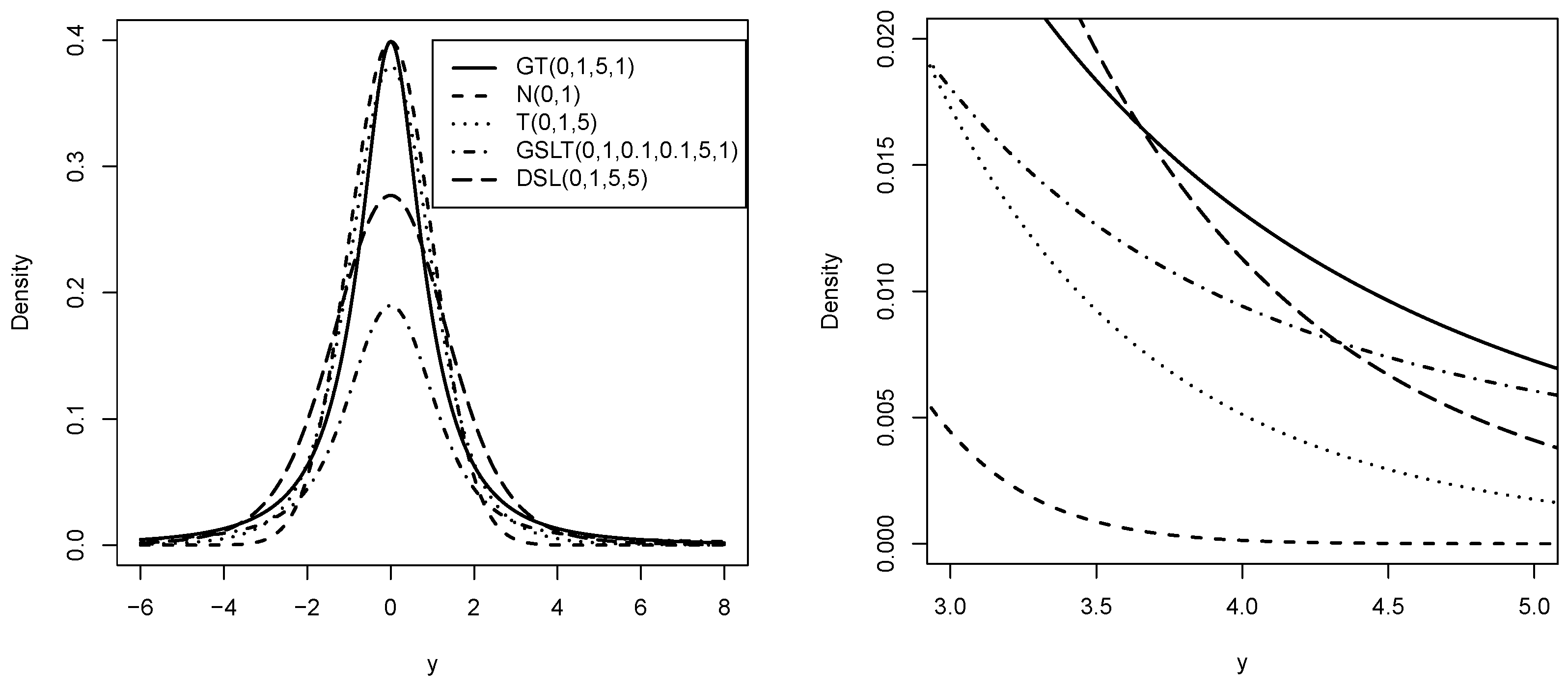
Another recent extension of the slash model was proposed by El-Morshedy, A. H. et al. [14]. These authors introduced the double slash (DSL) distribution with density function given by

$$\begin{array}{c}\hfill f_Y\left(y\right)=q_1{q}_2{\int }_0^1\left[{\int }_0^1\varphi \left(\left(\frac{y-\mu }{\sigma }\right)wt\right)t^{q_1}dt\right]w^{q_2}dw\end{array}$$

(9)

with $\mu \in \mathbb{R}$, $\sigma$, $q_1$ and $q_2>0$.

When $U\sim Ga(2\beta ,\beta )$ and $q=1$, in (1), the distribution generalized modified slash distribution, denoted $GMS(\mu ,\sigma ,\beta )$, studied by Reyes, J., Barranco-Chamorro, I., and Gómez, H. W. [15]. Whose function of density is given by

$$f_Y(y;\mu ,\sigma ,\beta )=\left\{\begin{array}{cc}\frac{1}{\sigma \sqrt{8\pi }}\hfill & \mathrm{if}y=\mu \hfill \\ \hfill & \\ \frac{2^{\beta /2}}{\sqrt{2\pi }}\frac{{\sigma }^{\beta +1}{\beta }^{\beta +2}}{{|y-\mu |}^{\beta +2}}U\left(1+\frac{\beta }{2},\frac{3}{2},\frac{2{\sigma }^2{\beta }^2}{{(y-\mu )}^2}\right)\hfill & \mathrm{if}y\ne \mu ,\hfill \end{array}\right.$$

(10)

where $\mu \in R$, $\sigma$, $\beta >0$ and

$$U(a,b,z)=\frac{1}{\mathsf{\Gamma }\left(a\right)}{\int }_0^{\infty }{t}^{a-1}{(1+t)}^{b-a-1}{e}^{-zt}dt,$$

(11)

is the confluent hypergeometric function of the second kind. Details about this function can be seen in Abramowitz and Stegun, p. 505.

With the motivation of finding a distribution that is a generalization of the student’s t distribution and that presents heavier tails than the distributions found so far in the literature, in this article, we introduce a new generalization of the student’s t distribution (GT) whose stochastic representation is given by

$$Y=\sigma \frac{W}{{(V/\nu )}^{1/q}}+\mu ,$$

(12)

where $W\sim N(0,1)$, $V\sim {\chi }_{\left(\nu \right)}^2$ are independent with $\nu >0$ and $q>0$ and we will denote it as $Y\sim GT(\mu ,\sigma ,\nu ,q)$.

The paper is organized as follows. In Section 2 the probability density function (pdf) is given and some properties of the $GT$ distribution are presented and shows that the distribution student’s t is a particular case of the distribution $GT$. Additionally, moments of order r are obtained, including the kurtosis coefficient. In Section 3 derivation of the moment and maximum likelihood estimators are discussed. A simulation study is presented to illustrate the behavior of the estimator of the parameters $\mu$, $\sigma$, and q, for $\nu =8$. Section 4 results of using the proposed model in two real applications are reported. Section 5 presents quantile regression. Section 6 presents the main conclusions.

2. The Generalized Student’s t Distribution

We present the generalized student’s t distribution with heavier tails compared to similar distributions. Initially we will present its density function.

2.1. Density Function

We will use the stochastic representation

$$\begin{array}{ccc}Y& =& \sigma \frac{W}{{(V/\nu )}^{1/q}}+\mu ,\end{array}$$

(13)

where W is distributed standard normal, V is distributed chi square, with $\nu$ degrees of freedom, W and V are independent random variables, $\mu$, $\sigma$ are location and scale parameters, respectively, $\nu$ degrees of freedom and $q>0$ is the parameter related to the distribution kurtosis.

We use the notation $Y\sim GT(\mu ,\sigma ,\nu ,q)$, and for the standard case, we denote $X\sim GT(0,1,\nu ,q)$.

Proposition 1.

Let $Y\sim GT(\mu ,\sigma ,\nu ,q)$. Then, the pdf of Y is given by

$$f_Y\left((y;\mu ,\sigma ,\nu ,q\right)=\left\{\begin{array}{ccc}\frac{1}{\sigma 2^{(\nu /2)}{\nu }^{1/q}\mathsf{\Gamma }(\nu /2)\sqrt{2\pi }}{\int }_0^{\infty }{t}^{\frac{\nu -2}{2}+\frac{1}{q}}{e}^{-\frac{1}{2}[{\left(\frac{y-\mu }{\sigma }\right)}^2{(t/\nu )}^{2/q}+t]}dt& & y\ne \mu \\ \frac{\mathsf{\Gamma }(\frac{\nu }{2}+\frac{1}{q})}{\sigma {(\nu /2)}^{1/q}\mathsf{\Gamma }(\nu /2)\sqrt{2\pi }}& & y=\mu .\end{array}\right.$$

(14)

Proof. 

Since W and V are two independent random variables, such that $W\sim N(0,1)$ and $V\sim {\chi }_{\left(\nu \right)}^2$, then the joint pdf of $\left(Y,T\right)=\left(\sigma W/{(V/\nu )}^{1/q}+\mu ,V\right)$ is

$$f_{(Y,T)}\left(y,t,\mu ,\sigma ,\nu ,q\right)=\frac{1}{\sigma 2^{(\nu /2)}{\nu }^{1/q}\mathsf{\Gamma }(\nu /2)\sqrt{2\pi }}{t}^{\frac{\nu -2}{2}+\frac{1}{q}}{e}^{-\frac{1}{2}[{\left(\frac{y-\mu }{\sigma }\right)}^2{(t/\nu )}^{2/q}+t]},$$

where $y\in \mathbb{R}$ and $t>0$. By marginalizing the result follows immediately para $y\ne \mu$. Doing $y=\mu$ the other expression is obtained. □

Corollary 1.

If $q=1$ in (14), then la fdp de Y is called the canonical generalized student’s t distribution.

$$f_Y\left(y;\mu ,\sigma ,\nu ,1\right)=\left\{\begin{array}{ccc}\frac{{\left(\frac{y-\mu }{\sigma }\right)}^{-\left(\frac{\nu }{2}+2\right)}{2}^{-3\left(1+\frac{\nu }{4}\right)}}{\sigma \sqrt{2\pi }}U\left[1+\frac{\nu }{4},\frac{3}{2},\frac{\nu }{{\left(\frac{y-\mu }{\sigma }\right)}^2}\right]& & y\ne \mu \\ \frac{1}{\sigma \sqrt{2\pi }}& & y=\mu ,\end{array}\right.$$

(15)

where $U(a,b,x)=\frac{1}{\mathsf{\Gamma }\left(a\right)}{\int }_0^{\infty }{e}^{-xt}{t}^{a-1}{(1+t)}^{b-a-1}dt$, it is called the second-class hypergeometric confluent function.

Proof. 

If $q=1$ in (14), then la fdp de Y is

$$f_Y\left((y;\mu ,\sigma ,\nu ,1\right)=\left\{\begin{array}{ccc}\frac{1}{\sigma 2^{(\nu /2)}\nu \mathsf{\Gamma }(\nu /2)\sqrt{2\pi }}{\int }_0^{\infty }{t}^{\frac{\nu }{2}}{e}^{-\frac{1}{2}[{\left(\frac{y-\mu }{\sigma }\right)}^2{(t/\nu )}^2+t]}dt& & y\ne \mu \\ \frac{1}{\sigma \sqrt{2\pi }}& & y=\mu .\end{array}\right.$$

(16)

Making $a=\nu /2$ and $b=\frac{{\left(\frac{y-\mu }{\sigma }\right)}^2}{{\nu }^2}$ and making the change of variables $w=\frac{t}{4a}$ and applying the result obtained in Reyes et al. [9]

$${\int }_0^{\infty }{t}^a{e}^{-\left(\frac{x^2}{2}{t}^2-2at\right)}dt=\frac{a\mathsf{\Gamma }(a+1)}{2^{a/2}{x}^{(a+2)}}U\left[1+\frac{a}{2},\frac{3}{2},\frac{a^2}{x^2}\right],$$

where $x=2\left(\frac{y-\mu }{\sigma }\right)$ the result is obtained. □

Figure 1 on the left shows the PDFs of the generalized student’s t distribution for q = 1 compared to the Student’s t for $\nu =5$, the normal distribution, the generalized bar t distribution and the double bar distribution. In which, it can be seen that as the variable tends to ∞ to the right (or to the left), the new model captures more data than the other comparative distributions. Furthermore, it is observed that to the extent that q is smaller, the distribution has greater kurtosis.

Figure 1. Generalized student’s pdf with $q=1$ (solid line), student’s for $\nu =5$ pdf (dotted line), Normal pdf (dashed line), $GSLT$ (dashed and dotted line) and $DSL$ (thick dashed line) (left), and tails comparison (right).

2.2. Tails Comparison of GT and Student’s t Distributions

In this part, we perform a comparison of the upper tails between the $GT$ distribution and student’s t distribution. For this, we consider the canonical version ($q=1$) of $GT$ distribution considering student’s t distribution with $\nu =5$ degrees of freedom. Table 1 shows $P(Y>y)$ for different values of y in the mentioned distributions. The $GT$ distribution has tails much heavier than the student’s t distribution.

Table 1. Tails comparison GT distributions and student’s t distribution.

Distribution	$\mathit{P}(\mathit{Y}>3)$	$\mathit{P}(\mathit{Y}>4)$	$\mathit{P}(\mathit{Y}>5)$	$\mathit{P}(\mathit{Y}>10)$
$T\left(5\right)$	0.0150	0.0052	0.0021	0.0001
$GT\left(5\right)$	0.0301	0.0103	0.0041	0.0002

Remark 1.

Table 1 illustrates the fact that the generalized student’s t distributions have heavier tails than the tails of the student’s t distribution.

2.3. Compared GT Quantiles with T Quantiles

Figure 2 shows the quantile function of the generalized student’s t distribution compared to quantile function of student’s t for different values of q and $\nu =5$.

Figure 2. Quantile function of the generalized student’s t distribution compared to quantile function of the student’s t for $\nu =5$ for $p=0.975$ (left) and $p=0.95$ (right).

Proposition 2.

Let $Y\sim GT(0,1,\nu ,q)$. Then an approximation of quantile p of Y is

$$y_p=\left\{\begin{array}{ccc}\frac{t_p}{2{\left(\frac{j_p}{\nu }\right)}^{\frac{q-2}{2q}}}\left[1+{\left(\frac{j_p}{\nu }\right)}^{\frac{q-2}{q}}\right]& & q<2\\ \frac{t_p}{{\left(\frac{j_p}{\nu }\right)}^{\frac{q-2}{2q}}}& & q>2,\end{array}\right.$$

where $t_p$ and $j_p$ denotes the quantiles p of student’s t and chi-square distribution whit ν degrees of freedom.

Proof. 

$Y=\frac{Z}{{\left(\frac{J}{\nu }\right)}^{\frac{1}{q}}}=\frac{Z}{{\left(\frac{J}{\nu }\right)}^{\frac{1}{2}}}\frac{{\left(\frac{J}{\nu }\right)}^{\frac{1}{2}}}{{\left(\frac{J}{\nu }\right)}^{\frac{1}{q}}}=T{\left(\frac{J}{\nu }\right)}^{\frac{2-q}{2q}}$

$⟹y_p\approx t_p{\left(\frac{J_p}{\nu }\right)}^{\frac{2-q}{2q}}$.

$Si$$q<2⟹y_p\approx t_p\left[\frac{{\left(\frac{J_p}{\nu }\right)}^{\frac{2-q}{2q}}+{\left(\frac{J_p}{\nu }\right)}^{\frac{q-2}{2q}}}{2}\right]$.

$Si$$q>2⟹y_p\approx \frac{t_p}{{\left(\frac{J_p}{\nu }\right)}^{\frac{q-2}{2q}}}$. □

Figure 3 shows the quantiles of the generalized student’s t distribution compared to quantile of proposition 2 for values $q=1$ and $\nu =5$.

Figure 3. Densidad de $GT$ evaluate in quantile theoretical compared to quantile, proposition 2 (upper), and qqplot (under).

Properties:

• If $q=2$ then $y_p=t_p$;
• if $\nu \to \infty$ then $y_p=z_p$ where $z_p$ is the quantile p of standard normal distribution.

In Table 2 we present quantiles generalized student’s t for n degrees of freedom and q = 1.

Table 2. Table of quantiles generalized student’s t for $\nu$ degrees of freedom and $q=1$.

$\mathit{\nu }$	${\mathit{GT}}_{0.60}$	${\mathit{GT}}_{0.70}$	${\mathit{GT}}_{0.80}$	${\mathit{GT}}_{0.90}$	${\mathit{GT}}_{0.95}$	${\mathit{GT}}_{0.975}$	${\mathit{GT}}_{0.99}$	${\mathit{GT}}_{0.995}$
1	0.330	0.727	1.419	3.467	7.798	17.074	47.159	100.682
2	0.289	0.620	1.091	2.052	3.371	5.252	9.096	13.578
3	0.277	0.587	1.002	1.749	2.628	3.710	5.583	7.453
4	0.271	0.571	0.960	1.619	2.334	3.149	4.442	5.631
5	0.267	0.562	0.936	1.546	2.176	2.861	3.891	4.791
6	0.265	0.556	0.920	1.499	2.078	2.687	3.569	4.314
7	0.263	0.551	0.909	1.467	2.011	2.570	3.358	4.006
8	0.262	0.548	0.900	1.443	1.962	2.486	3.209	3.792
9	0.261	0.545	0.894	1.425	1.925	2.422	3.098	3.634
10	0.260	0.543	0.889	1.410	1.896	2.373	3.012	3.513
11	0.260	0.542	0.884	1.398	1.872	2.333	2.944	3.418
12	0.259	0.540	0.881	1.389	1.853	2.300	2.888	3.340
13	0.259	0.539	0.878	1.380	1.836	2.273	2.842	3.276
14	0.258	0.538	0.875	1.373	1.823	2.250	2.803	3.221
15	0.258	0.537	0.873	1.367	1.811	2.230	2.769	3.175
16	0.258	0.536	0.871	1.362	1.800	2.213	2.740	3.135
17	0.257	0.536	0.870	1.357	1.791	2.197	2.715	3.100
18	0.257	0.535	0.868	1.353	1.783	2.184	2.692	3.070
20	0.257	0.534	0.865	1.346	1.769	2.161	2.655	3.018
21	0.257	0.534	0.864	1.343	1.763	2.152	2.639	2.996
22	0.256	0.533	0.863	1.340	1.758	2.143	2.624	2.976
23	0.256	0.533	0.862	1.338	1.753	2.135	2.611	2.958
24	0.256	0.532	0.861	1.335	1.748	2.127	2.599	2.942
25	0.256	0.532	0.861	1.333	1.744	2.121	2.588	2.927
26	0.256	0.532	0.860	1.331	1.740	2.114	2.577	2.913
27	0.256	0.532	0.859	1.329	1.737	2.109	2.568	2.900
28	0.256	0.531	0.859	1.328	1.734	2.103	2.559	2.888
29	0.256	0.531	0.858	1.326	1.730	2.098	2.551	2.877
30	0.256	0.531	0.858	1.325	1.728	2.094	2.544	2.867

2.4. Properties of the Generalized Student’s t Distribution

In this section, we present some properties of the generalized student’s t distribution.

Proposition 3.

Let $Y\sim GT(\mu ,\sigma ,\nu ,q)$ then

1. 

$\underset{q\to \infty }{lim}{f}_Y\left(y;\mu ,\sigma ,\nu ,q\right)=\frac{1}{\sigma }\varphi \left(\frac{y-\mu }{\sigma }\right)$.

2. 

If $Y|V=v\sim N(\mu ,v^{-2/q}{\sigma }^2)$ and $V\sim {\chi }_{\left(\nu \right)}^2$ then $Y\sim GT(\mu ,\sigma ,\nu ,q)$.

3. 

If $Y\sim GT(0,1,\nu ,2)$, then, $Y\sim t_{\left(\nu \right)}$.

Proof. 

• Making q tend to infinity in representation (13), the result is immediately obtained;
• $f_Y(y;\mu ,\sigma ,\nu ,q)={\int }_0^{\infty }\varphi (y;\mu ,v^{-1/q}\sigma )f_V\left(v\right)dv={\int }_0^{\infty }\frac{v^{1/q}}{\sigma }\varphi \left(\frac{y-\mu }{\sigma v^{-1/q}}\right)f_V\left(v\right)dv$. where $f_V$ es la fdp chi-square distribution with $\nu$ degrees of freedom. The result follows using transformation $t=v^{1/q}$ and direct integral computations;
• Making $q=2$ we obtain the density student’s with $\nu$ degrees of freedom.

□

Remark 2.

Proposition 3 shows first that the generalized student’s t distribution contains the normal distribution as a special case ($q\to \infty$). Moreover, it also shows that the generalized student’s t distribution is a scale mixture between the normal and the chi-square distribution with ν degrees of freedom. The third property shows that for $q=2$, the density function for the generalized student’s t coincides with the density function of the student’s t distribution with ν degrees of freedom.

2.5. Moments

In this subsection the moments of the generalized student’s t distribution are deduced.

Proposition 4.

Let $X\sim GT(0,1,\nu ,q)$ and $Y\sim GT(\mu ,\sigma ,\nu ,q)$. Hence, for $r=1,2,3,....$ and $q>2r/\nu$, we have that

$${\mu }_{2r}=E\left(X^{2r}\right)=\frac{{\nu }^{\frac{2r}{q}}{2}^{2r\frac{q+1}{q}}\left(2r\right)!\mathsf{\Gamma }(\frac{\nu }{2}-\frac{2r}{q})}{r!\mathsf{\Gamma }(\nu /2)}{\mu }_{2r-1}=E\left(X^{2r-1}\right)=0$$

and

$$\begin{array}{ccc}E\left(Y^r\right)& =& {\displaystyle \sum _{k=0}^r}\left(\begin{array}{c}r\\ k\end{array}\right){\sigma }^k{\mu }^{r-k}{\mu }_k.\end{array}$$

Proof. 

Representation (13) with $\mu =0$ and $\sigma =1$, and since W and V are independent, we have that

$${\mu }_{2r}=E\left(X^{2r}\right)=E\left({\left(\frac{W}{{(V/\nu )}^{1/q}}\right)}^{2r}\right)=E\left(W^{2r}\right)E\left({(V/\nu )}^{-2r/q}\right).$$

Moreover, since $E\left({(V/\nu )}^{-2r/q}\right)={\nu }^{2r/q}E\left(V^{-2r/q}\right)={\nu }^{2r/q}{2}^{-2r/q}\frac{\mathsf{\Gamma }\left(\frac{\nu }{2}-\frac{2r}{q}\right)}{2^{2r/q}\mathsf{\Gamma }(\nu /2)},q>2r/\nu$ and $E\left(W^{2r}\right)=\frac{\left(2r\right)!}{2^{r}r!}$ are even moments for the standard normal distribution, the second result follows directly by applying the formula to the stochastic representation (13). □

Corollary 2.

Let $Y\sim GT(\mu ,\sigma ,\nu ,q)$, and hence,

$$E\left(Y\right)=\mu andVar\left(Y\right)=\frac{2{\sigma }^2{\nu }^{2/q}{2}^{2\frac{q+2}{q}}\mathsf{\Gamma }\left(\frac{\nu }{2}-\frac{2}{q}\right)}{\mathsf{\Gamma }(\nu /2)},q>4/\nu .$$

(17)

Proposition 5.

Let $Y\sim GT(\mu ,\sigma ,\nu ,q)$, so that the coefficient of skewness and kurtosis are:

$${\gamma }_1=0$$

(18)

and

$${\beta }_2=\frac{3\mathsf{\Gamma }(\nu /2)\mathsf{\Gamma }\left(\frac{\nu }{2}-\frac{4}{q}\right)}{{\mathsf{\Gamma }}^2\left(\frac{\nu }{2}-\frac{2}{q}\right)},q>8/\nu .$$

(19)

Proof. 

The standardized coefficient of skewness and kurtosis are

$${\gamma }_1=\frac{{\mu }_3-3{\mu }_1{\mu }_3+2{\mu }_1^3}{{({\mu }_2-{\mu }_1^2)}^{3/2}}$$

and

$${\beta }_2=\frac{{\mu }_4-4{\mu }_1{\mu }_3+6{\mu }_1^2{\mu }_2-3{\mu }_1^4}{{({\mu }_2-{\mu }_1^2)}^2}$$

and the result follows after replacing the even moments derived in Proposition 4. □

Figure 4 shows the kurtosis the $GT$ distribution compared with T distribution for different values of q and $\nu =8$.

Figure 4. Kurtosis of the $GT$ distribution compared with T distribution for $\nu =8$.

It can be seen that the generalized student’s distribution has a greater kurtosis than the student’s distribution for q less than 2, then for data with high kurtosis, it would be recommended to use the generalized student’s distribution.

3. Inference

3.1. Moment Estimators

In the following proposition we present the moment estimators of $\mu$, $\sigma$, and q for $\nu =8$.

Proposition 6.

Where $Y_1,\cdots ,Y_n$ a random sample from the distribution of the random variable $Y\sim GT(\mu ,\sigma ,\nu ,q)$, so that the moment estimators of $\theta =(\mu ,\sigma ,\nu ,q)$ for $q>1$ are given by

$${\widehat{\mu }}_M=\overline{Y},{\widehat{\sigma }}_M={\left(\frac{\mathsf{\Gamma }(\nu /2)S^2}{2{\nu }^{2/{\widehat{q}}_M}{2}^{2\frac{q+2}{q}}\mathsf{\Gamma }(\frac{\nu }{2}-\frac{2}{{\widehat{q}}_M})}\right)}^{1/2}and {\gamma }_2=\frac{3\mathsf{\Gamma }(\nu /2)\mathsf{\Gamma }(\frac{\nu }{2}-\frac{4}{{\widehat{q}}_M})}{{\mathsf{\Gamma }}^2(\frac{\nu }{2}-\frac{2}{{\widehat{q}}_M})},\nu >\frac{8}{q}o \nu >8 and q<1$$

where $\overline{Y}$, S and ${\gamma }_2$ are the mean, standard deviation, and sample kurtosis coefficient.

Proof. 

Using (17) it follows that

$$\mu =E\left(Y\right)and{\sigma }^2=\frac{\mathsf{\Gamma }(\nu /2)Var\left(Y\right)}{2{\nu }^{2/q}{4}^{\frac{q+2}{q}}\mathsf{\Gamma }\left(\frac{\nu }{2}-\frac{2}{q}\right)}$$

(20)

replacing ${\gamma }_2$ in (19) one obtains the numerical equation

$${\gamma }_2=\frac{3\mathsf{\Gamma }(\nu /2)\mathsf{\Gamma }(\frac{\nu }{2}-\frac{4}{{\widehat{q}}_M})}{{\mathsf{\Gamma }}^2(\frac{\nu }{2}-\frac{2}{{\widehat{q}}_M})}$$

(21)

and solving (21) for $\widehat{q}$ and $\widehat{\nu }$ one obtains ${\widehat{q}}_M$ and ${\widehat{\nu }}_M$. Further, replacing in (20) q by ${\widehat{q}}_M$, $\nu$ by ${\widehat{\nu }}_M$, $E\left(Y\right)$ by $\overline{Y}$ and $Var\left(Y\right)$ by the sample variance $S^2$, we obtain the moment estimators $({\widehat{\mu }}_M,{\widehat{\sigma }}_M,{\widehat{\nu }}_M,{\widehat{q}}_M)$ for $(\mu ,\sigma ,\nu ,q)$. □

3.2. Maximum Likelihood Estimation

Given a random sample $Y_i\sim GT(\mu ,\sigma ,\nu ,q)$, for $i=1,..,n$, the log-likelihood function can be written as

$$l(\mu ,\sigma ,\nu ,q)=-nlog\left(\sigma \right)-\frac{n\nu }{2}\log \left(2\right)-\frac{n}{q}log\left(\nu \right)-nlog\left(\mathsf{\Gamma }(\nu /2)\right)-\frac{n}{2}log\left(2\pi \right)+\sum _{i=1}^{n}logG\left(y_i\right)$$

(22)

where $G\left(y_i\right)=G(y_i;\mu ,\sigma ,\nu ,q)={\int }_0^{\infty }{v}^{\frac{\nu -2}{2}+\frac{1}{q}}{e}^{-\frac{1}{2}[{\left(\frac{y_i-\mu }{\sigma }\right)}^2{\left(\frac{v}{\nu }\right)}^{\frac{2}{q}}+v]}dv$ and hence the maximum likelihood equations are given by

$$\begin{array}{ccc}\hfill \sum _{i=1}^n\frac{G_1\left(y_i\right)}{G\left(y_i\right)}& =& 0\hfill \end{array}$$

(23)

$$\begin{array}{ccc}\hfill \sum _{i=1}^n\frac{G_2\left(y_i\right)}{G\left(y_i\right)}& =& \frac{n}{\sigma }\hfill \end{array}$$

(24)

$$\begin{array}{ccc}\hfill \hspace{1em}\hspace{1em}\hspace{1em}\hspace{1em}\hspace{1em}\hspace{1em}\hspace{1em} \hspace{1em}\sum _{i=1}^n\frac{G_3\left(y_i\right)}{G\left(y_i\right)}& =& \frac{nlog\left(2\right)}{2}+\frac{n}{q\nu }+\frac{n\mathsf{\Psi }(\nu /2)}{2}\hfill \end{array}$$

(25)

$$\begin{array}{ccc}\hfill \hspace{1em}\hspace{1em} \sum _{i=1}^n\frac{G_4\left(y_i\right)}{G\left(y_i\right)}& =& -\frac{nlog\left(\nu \right)}{q^2}\hfill \end{array}$$

(26)

where, $G_1\left(y_i\right)=\frac{\partial }{\partial \mu }G\left(y_i\right)$, $G_2\left(y_i\right)=\frac{\partial }{\partial \sigma }G\left(y_i\right)$, $G_3\left(y_i\right)=\frac{\partial }{\partial \nu }G\left(y_i\right)$. $G_4\left(y_i\right)=\frac{\partial }{\partial q}G\left(y_i\right)$. The expressions for $G_1\left(y_i\right)$, $G_2\left(y_i\right)$, $G_3\left(y_i\right)$ and $G_4\left(y_i\right)$ should be given,

$$\begin{array}{ccc}\hfill G_1\left(y_i\right)& =& \frac{1}{\sigma 2{\nu }^{\frac{1}{q}}}{\int }_0^{\infty }(y_i-\mu )t_i\left(\nu \right)dv\hfill \end{array}$$

(27)

$$\begin{array}{ccc}\hfill G_2\left(y_i\right)& =& \frac{1}{\sigma 3{\nu }^{\frac{2}{q}}}{\int }_0^{\infty }{(y_i-\mu )}^2{t}_i\left(\nu \right)dv\hfill \end{array}$$

(28)

$$\begin{array}{ccc}\hfill \hspace{1em}\hspace{1em} \hspace{0.17em} \hspace{1em}\hspace{1em}\hspace{1em}{G}_3\left(y_i\right)& =& \frac{1}{q\sigma 2\nu }{\int }_0^{\infty }[{\frac{v}{\nu }}^{2/q}{(y_i-\mu )}^2+q{\sigma }^2\nu \log \left(v\right)t_i\left(\nu \right)dv\hfill \end{array}$$

(29)

$$\begin{array}{ccc}\hfill \hspace{1em}\hspace{1em} \hspace{0.17em} \hspace{1em}\hspace{1em}\hspace{1em}\hspace{1em}\hspace{1em}\hspace{1em}\hspace{1em} \hspace{1em}{G}_4\left(y_i\right)& =& -\frac{1}{\sigma 2q^2}{\int }_0^{\infty }[{\sigma }^2\log \left(v\right)-\log (v/q){(v/q)}^{2/q}{(y_i-\mu )}^2]t_i\left(\nu \right)dv,\hfill \end{array}$$

(30)

where $t_i\left(\nu \right)=v^{\frac{\nu -2}{2}+\frac{1}{q}}{e}^{-\frac{1}{2}[{\left(\frac{y_i-\mu }{\sigma }\right)}^2{\left(\frac{v}{\nu }\right)}^{\frac{2}{q}}+v]}$.

Using numerical procedures Equations (27)–(30) can be solved.

Proposition 7.

Let $Y_1,\cdots ,Y_n$ a random sample from the distribution of random variable $Y\sim GT(\mu ,\sigma ,\nu ,q)$. Then,

$$Y=\left(\frac{\overline{Y}-\mu }{S^{2/q}{\sigma }^{1-2/q}}\right)\sqrt{n}\sim GT(0,1,\nu ,q)$$

(31)

Proof. 

The random variable Z and T

$$Z=\frac{\overline{Y}-\mu }{\sigma \sqrt{n}}\sim N(0,1)$$

$$T=\frac{(n-1)S^2}{{\sigma }^2}\sim {\chi }_{(n-1)}^2$$

then

$$Y=\frac{Z}{{(T/(n-1))}^{1/q}}\sim GT(0,1,\nu ,q)$$

replacing the result is obtained. □

Proposition 8.

Let $Y_1,\cdots ,Y_n$ a random sample from the distribution of random variable $Y\sim GT(\mu ,\sigma ,\nu ,q)$. Then, a level $(1-\alpha )$ confidence interval for the population mean is

$$[\overline{Y}-t_{1-\alpha /2}^{\prime }\frac{S^{2/q}{\sigma }^{1-2/q}}{\sqrt{n}},\overline{Y}+t_{1-\alpha /2}^{\prime }\frac{S^{2/q}{\sigma }^{1-2/q}}{\sqrt{n}}],$$

where $t_{1-\alpha /2}^{\prime }$ is the percentile of order $1-\frac{\alpha }{2}$ of GT distribution.

Proof. 

The result is obtained from the previous proposition. □

3.3. Simulation Study

To generate random numbers from the $GT(\mu ,\sigma ,8,q)$ distribution we will use the stochastic representation given in (13) and the following algorithm:

• Simulate $Z\sim N(0,1);$
• Simulate $V\sim {\chi }^2\left(\nu \right);$
• Compute $Y=\sigma \frac{Z}{{(V/\nu )}^{1/q}}+\mu .$

It then follows that $Y\sim GT(\mu ,\sigma ,\nu ,q)$.

Table 3 shows the parameter estimates obtained by the maximum likelihood method (MLE) through 1000 replicates of sizes 50, 100, 150, and 200 with their corresponding standard errors, mean length of the interval, and empirical coverage.

Table 3. Simulation of 1000 iterations of the model $GT(\mu ,\sigma ,8,q)$.

n	$\mathit{\mu }$	$\mathit{\sigma }$	q	$\widehat{\mathit{\mu }}$	$\mathit{sd}\left(\widehat{\mathit{\mu }}\right)$	$\mathit{ali}\left(\widehat{\mathit{\mu }}\right)$	$\mathit{c}\left(\widehat{\mathit{\mu }}\right)$	$\widehat{\mathit{\sigma }}$	$\mathit{sd}\left(\widehat{\mathit{\sigma }}\right)$	$\mathit{ali}\left(\widehat{\mathit{\sigma }}\right)$	$\mathit{c}\left(\widehat{\mathit{\sigma }}\right)$	$\widehat{\mathit{q}}$	$\mathit{sd}\left(\widehat{\mathit{q}}\right)$	$\mathit{ali}\left(\widehat{\mathit{q}}\right)$	$\mathit{c}\left(\widehat{\mathit{q}}\right)$
50	0.5	1	1	0.4992	0.1665	0.6527	96.10	0.9958	0.1760	0.6899	94.80	1.1558	0.5080	1.9914	92.80
100				0.5018	0.1148	0.4502	94.50	1.0012	0.1237	0.4851	94.30	1.0961	0.3319	1.3009	94.20
150				0.5045	0.0965	0.3785	95.50	1.0016	0.0967	0.3791	95.20	1.0542	0.2576	1.0098	95.00
200				0.5003	0.0801	0.3138	95.80	1.0018	0.0822	0.3221	95.10	1.0442	0.1908	0.7481	94.70
50	1	1	1	1.0002	0.1649	0.6462	95.90	0.9963	0.1723	0.6756	94.90	1.1580	0.5084	1.9931	92.80
100				1.0007	0.1190	0.4664	95.10	1.0003	0.1277	0.5005	94.80	1.0948	0.3340	1.3094	94.10
150				1.0045	0.0966	0.3785	95.50	1.0016	0.0967	0.3790	95.20	1.0540	0.2575	1.0093	95.00
200				1.0003	0.0801	0.3138	95.80	1.0018	0.0822	0.3222	95.10	1.0442	0.1908	0.7479	94.70
50	1	2	1	0.9998	0.3311	1.2979	96.00	1.9893	0.3506	1.3743	94.90	1.1511	0.4939	1.9363	92.90
100				1.0037	0.2290	0.8978	94.60	2.0035	0.2467	0.9670	94.70	1.0964	0.3247	1.2729	93.80
150				1.0094	0.1929	0.7560	95.50	2.0043	0.1935	0.7584	94.90	1.0552	0.2548	0.9989	95.20
200				1.0004	0.1601	0.6276	95.80	2.0044	0.1639	0.6425	94.90	1.0445	0.1893	0.7420	94.70
50	1	3	1	0.9337	0.5396	2.1153	97.70	2.7991	0.8856	3.4714	93.60	1.0815	0.5529	2.1675	94.80
100				1.0042	0.3448	1.3516	94.70	3.0016	0.3818	1.4966	94.90	1.0970	0.3373	1.3222	94.10
150				1.0135	0.2893	1.1342	95.10	3.0082	0.2903	1.1381	95.10	1.0568	0.2563	1.0045	95.00
200				0.9997	0.2416	0.9472	95.70	3.0059	0.2630	1.0308	96.60	1.0456	0.1950	0.7643	95.20
50	0.5	0.5	1	0.5000	0.0825	0.3235	95.90	0.4986	0.0873	0.3422	94.70	1.1629	0.5318	2.0848	93.60
100				0.5003	0.0577	0.2261	94.70	0.5006	0.0620	0.2431	94.40	1.0954	0.3285	1.2878	94.10
150				0.5020	0.0482	0.1889	95.30	0.5007	0.0484	0.1899	94.80	1.0544	0.2573	1.0086	95.00
200				0.5000	0.0400	0.1567	96.00	0.5011	0.0412	0.1617	95.00	1.0445	0.1935	0.7585	94.60
50	1	0.5	1	1.0000	0.0825	0.3236	95.90	0.4987	0.0872	0.3420	94.70	1.1662	0.5413	2.1219	93.60
100				1.0004	0.0576	0.2260	94.60	0.5006	0.0620	0.2431	94.40	1.0960	0.3286	1.2880	94.10
150				1.0020	0.0482	0.1890	95.50	0.5008	0.0483	0.1895	94.70	1.0547	0.2572	1.0081	95.00
200				0.9999	0.0400	0.1567	95.90	0.5010	0.0414	0.1621	94.90	1.0461	0.1955	0.7663	94.70
50	1	0.5	0.5	1.0002	0.0695	0.2725	95.40	0.5045	0.1138	0.4462	94.70	0.5252	0.1355	0.5312	95.10
100				1.0005	0.0479	0.1879	94.00	0.5003	0.0798	0.3127	94.80	0.5131	0.0750	0.2941	94.80
150				1.0019	0.0389	0.1527	95.70	0.5022	0.0609	0.2388	94.10	0.5070	0.0587	0.2301	94.90
200				1.0003	0.0327	0.1281	95.20	0.5016	0.0544	0.2131	96.10	0.5070	0.0520	0.2038	94.60
50	0.5	0.5	0.5	0.5001	0.0695	0.2724	95.40	0.5040	0.1139	0.4467	94.70	0.5249	0.1355	0.5313	95.10
100				0.5007	0.0481	0.1885	94.20	0.5011	0.0800	0.3137	94.80	0.5135	0.0752	0.2949	94.80
150				0.5020	0.0390	0.1529	95.70	0.5021	0.0610	0.2393	94.20	0.5070	0.0587	0.2303	94.90
200				0.5001	0.0329	0.1290	95.10	0.5016	0.0544	0.2132	96.00	0.5073	0.0520	0.2038	94.60

$sd$ corresponds to the standard deviation, average length of interval ($ali$) is the average length of the confidence interval and c the empirical coverage of the respective EMV of the parameters, based on a $95\%$ confidence interval.

4. Two Illustrative Datasets

Illustrative Datasets 1

We consider the data that were first presented in Jander [16], from an entomology experiment. with respect to ants. A total of $n=730$ ants were individually placed in the center of an arena. The measurements correspond to the initial direction in which they moved relative to a visual stimulus in a 180 degree angle from zero direction, rounded to the nearest 10 grades. Figure 5 depicts the histogram of these data, including estimated densities under a T, $ES$, $MS$, $SGT$, $DSL$ and $GT$ model, using maximum likelihood. Figure 6 shows the qqplots for T, $ES$, $MS$ and $GT$ models. We use the AIC (Akaike Information Criterion), which penalizes the maximized likelihood function by the excess of model parameters (AIC = −2log(lik) + 2k, where k is the number of unknown parameters being estimated, see Akaike [17]). Table 4 shows the descriptive statistics of the database, while Table 5 presents the Kolmogorov -Smirnov (KSS) statistic, corresponding values for the four given models, which also indicates that the best fit is presented by the $GT$ model. Table 6 shows a 95% confidence interval for the population mean using generalized Student’s t-quantiles. Moreover, Figure 7 depicts the empirical cumulative distribution function (cdf) and the estimated cdfs for T, $ES$, $MS$ and $GT$ models.

Figure 5. Histogram (left) and Comparison the tails (right) for ants dataset. Overlaid on top is the generalized student’s t density with parameters estimated via ML (solid line), the modified slash density (dashed line), the extended slash density (dotted line), the student’s t density (dashed line).

Figure 6. Q-q plots: student’s t (a), modified slash (b), extended slash (c), generalized student’s t (d).

Table 4. Descriptive statistics the for dataset.

n	$\overline{\mathit{X}}$	S	$\sqrt{{\mathit{b}}_1}$	${\mathit{b}}_2$
730	$176.438$	$62.6434$	$-0.2057$	$4.6071$

Table 5. Parameter estimates, AIC and KSS values for T, $MS$, $ES$, and $GT$ models for the ants dataset.

Parameter	T	MS	ES	GT
$\mu$	181.58 (1.265)	181.67 (1.217)	181.321 (0.094)	181.4824 (1.1466)
$\sigma$	26.142 (1.712)	16.7 (0.878)	1.336 (0.108)	33.4038 (1.5802)
$\nu$	1.47 (0.134)			18.7203 (0.0029)
q		1.50 (0.034)		0.4085 (0.0013)
$\alpha$			1.907 (0.094)
$\beta$			40.084 (4.719)
AIC	7928.448	7921.282	7914.642	7899.405
KSS	0.1174	0.0781	0.1000	0.0644
p-value	0.0005	0.0117	0.0007	0.4850

Table 6. The 95 percent confidence interval for the mean of dataset using T and $GT$ quantiles T.

Distribution	Lower Limit	Upper Limit
T	170.5121	182.4633
$GT$	166.8242	186.1511

Figure 7. Empirical cdf with estimated T c.d.f. (yellow color),estimated $MS$ cdf (red color), estimated $ES$ c.d.f. (green color), and estimated $GT$ c.d.f. (blue color).

The estimators of moments for the dataset are:

• ${\widehat{\mu }}_M=170.438$;
• ${\widehat{\sigma }}_M=47.551$;
• ${\widehat{\nu }}_M=9.3458$;
• ${\widehat{q}}_M=0.4868$,

which will be used as starting points in obtaining the EMVs.

Figure 8 depicts the histogram of these data, including estimated densities under a $SGT$, $DSL$ and $GT$ model, using maximum likelihood. We use the Akaike information criterion (AIC) and Bayesian Information Criterion (BIC), see Schwarz [18], which is defined as (BIC = $-2log\left(lik\right)+klog\left(n\right)$, where k is the number of estimated parameters and n is the sample size. Table 7 shows these results.

Figure 8. Histogram (left) and comparison the tails (right) for ants dataset. Overlaid on top is the generalized student’s t density with parameters estimated via ML (solid line), the modified slash density (dashed line), the extended slash density (dotted line),the student’s t density (dashed line).

Table 7. Parameter estimates, AIC and BIC values for $GSLT$, $DSL$ and $GT$ models for the ants dataset.

Parameter	$\mathit{DSL}$	$\mathit{GSLT}$	$\mathit{GT}$
$\mu$	181.6341 (1.2443)	180.0680 (0.0169)	181.4824 (1.1466)
$\sigma$	11.9447 (1.10722)	2.5871 (0.0168)	33.4038 (1.5802)
$\nu$		2.2523 (0.0168	18.7203 (0.0029)
$q_1$	1.6916 (0.2390)	0.4774 (0.0069)	0.4085 (0.0013)
$q_2$	1.6911 (0.2788)		0.4085 (0.0013)
$\alpha$	12.9451 (0.0169)
$\beta$	28.0256 (0.0170)
AIC	7931.313	7915.774	7899.405
BIC	7949.745	7943.333	7902.14

5. Quantile Regression

The quantile regression is used when the study objective focuses on the estimation of the different percentiles (such as the median) of a population of interest. An advantage of using quantile regression to estimate the median, rather than ordinary least squares regression current file (to estimate the mean), is that the quantile regression will be more robust in the presence of outliers. Quantile regression can be seen as a natural analogue in regression analysis when using different measures of central tendency and dispersion, in order to obtain a more complete and robust analysis of the data. Another advantage of this type of regression lies in the possibility of estimating any quantile, thus being able to assess what happens with extreme values of the population.

5.1. Quantile Regression Uni-Dimensional

Translating this concept of quantile to the regression line, we obtain the linear quantile regression.

If we assume that

$$Y_i={\beta }_{0,\tau }+{\beta }_{1,\tau }{X}_i+{ϵ}_{i,\tau },$$

$\forall iϵ(1,...,n)$ with $\tau ϵ(0,1)$ and that the conditional expected value is not necessarily zero, but the $\tau$-ésimo quantile of the error with respect to the regressive variable is zero $(Q_{\tau }({ϵ}_{i,\tau }/X)=0)$, then the $\tau$-ésimo quantile of $Y_i$ with respect to X can be written as

$$Q_{\tau }(Y_i/X)={\beta }_{0,\tau }+{\beta }_{1,\tau }{X}_i$$

The estimates of ${\beta }_{0,\tau }$ y ${\beta }_{1,\tau }$ are found by

$$\widehat{{\beta }_{\tau }}=arg\underset{{\beta }_{\tau }ϵ{\Re }^2}{min}\left(\sum _{Y_i\ge A}\tau |Y_i-{\beta }_{0,\tau }-{\beta }_{1,\tau }{X}_i|+\sum _{Y_i<A}(1-\tau )|Y_i-{\beta }_{0,\tau }-{\beta }_{1,\tau }{X}_i|\right),$$

(32)

being ${\beta }_{\tau }=({\beta }_{0,\tau },{\beta }_{1,\tau })$ y $A={\beta }_{0,\tau }+{\beta }_{1,\tau }{X}_i$.

To estimate the parameters, the function described in the equation should be minimized. For this, there is a way to approach the minimization problem as a linear programming problem. This allows us to obtain the regression line for the value of a certain quantile. Therefore, the first of the limitations will be solved raised at the end of the previous section, for simple linear regression. Furthermore, since the quartiles have robust properties, it is also possible to solve the second of the limitations that arose with the classical regression line.

5.2. Quantile Regression Student’s t

In this case, in the regression equation

$$Y_i={\beta }_{0,\tau }+{\beta }_{1,\tau }{X}_i+{ϵ}_{i,\tau },$$

$\forall iϵ(1,...,n)$ the response variable $Y\sim T(\mu ,\sigma ,\nu )$, it is possible to generate random numbers for the $T(\mu ,\sigma ,\nu )$ distribution, which the parameters $\mu$, $\sigma$ and $\nu$ they are estimated using maximum likelihood for the data. Then, one way to obtain the quantiles of Y is using the stochastic representation.

• Simulate $W\sim N(0,1)$;
• Simulate $T\sim {\chi }^2\left(\nu \right);$
• Compute $Y_1=\sigma \left(\frac{W}{{(T/\nu )}^{1/2}}\right)+\mu .$

Using this new variable $Y_1$ quantile regression is applied to the data $(X,Y_1)$.

5.3. Quantile Regression Slash Logistic

In this case, in the regression equation

$$Y_i={\beta }_{0,\tau }+{\beta }_{1,\tau }{X}_i+{ϵ}_{i,\tau },$$

$\forall iϵ(1,...,n)$ the response variable $Y\sim GSLOG(\mu ,\sigma ,q)$, it is possible to generate random numbers for the $SLOG(\mu ,\sigma ,q)$ distribution, which the parameters $\mu$, $\sigma$, and q they are estimated using maximum likelihood for the data. Then, one way to obtain the quantiles of Y is using the stochastic representation.

• Simulate $W\sim U(0,1)$;
• Compute $T=\mu +\sigma \log \left(\frac{W}{1-W}\right)$;
• Simulate $U\sim U(0,1)$;
• Compute $Y_2=\frac{T}{U^{1/q}}$.

Using this new variable $Y_2$ quantile regression is applied to the data $(X,Y_2)$.

5.4. Quantile Regression Generalized Student’s t

In this case, in the regression equation

$$Y_i={\beta }_{0,\tau }+{\beta }_{1,\tau }{X}_i+{ϵ}_{i,\tau },$$

$\forall iϵ(1,...,n)$ the response variable $Y\sim GT(\mu ,\sigma ,\nu ,q)$, it is possible to generate random numbers for the $GT(\mu ,\sigma ,\nu ,q)$ distribution, which the parameters $\mu$, $\sigma$, $\nu$, and q they are estimated using maximum likelihood for the data. Then, one way to obtain the quantiles of Y is using the stochastic representation given in (13)

• Simulate $W\sim N(0,1)$;
• Simulate $T\sim {\chi }^2\left(\nu \right);$
• Compute $Y_3=\sigma \left(\frac{W}{{(T/\nu )}^{1/q}}\right)+\mu .$

Using this new variable $Y_3$ quantile regression is applied to the data $(X,Y_3)$.

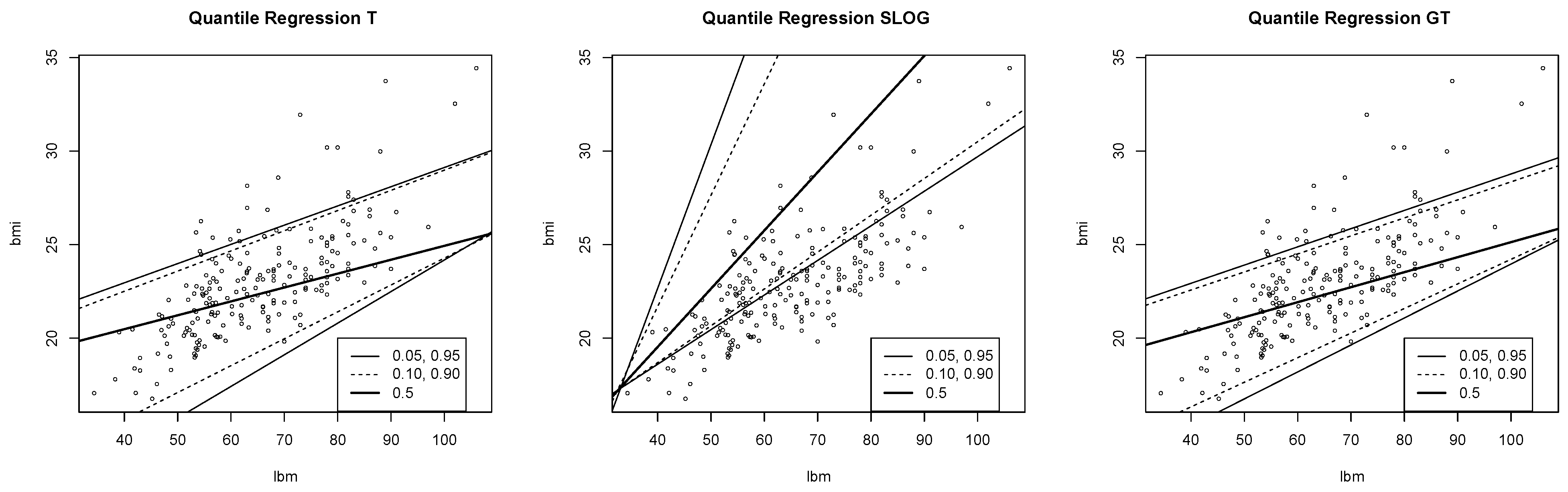
5.5. Application 2

We consider now data concerning the body mass index and Lean Body Mass of 202 Australian athletes. The data are available for download at http://azzalini.stat.unipd.it/SN/index.html (accessed on 15 October 2021). Table 8 shows statistics for these data for which the maximum likelihood estimators of (${\beta }_0$, ${\beta }_1$) and its corresponding coefficients AIC and BIC fit models for data. are shown in Table 9 and Table 10, respectively.

Table 8. Summary statistics for dataset of the body mass index and Lean Body Mass of 202 Australian athletes.

Data	n	$\overline{\mathit{W}}$	${\mathit{S}}_{\mathit{W}}$	$\sqrt{{\mathit{\beta }}_1}$	${\mathit{\beta }}_2$
BMI	202	22.9264	2.8664	0.9395	5.1323
LBM	202	64.8767	13.0702	0.3558	2.7326

Table 9. Coefficients AIC and BIC fit models for dataset of the body mass index and Lean Body Mass of 202 Australian athletes for quantile regression student’s t (T), quantile regression slash logistic (SLOG) and quantile regression generalized student’s t (GT).

Coef.	T	SLOG	GT
AIC	915.309	1252.004	904.573
BIC	925.234	1261.928	914.498

Table 10. Parameter estimates and standard deviation values for quantile regression coefficients 50 student’s t (T) and generalized student’s t ($GT$) models for the dataset.

Distribution	Coef.	Est.	SD	t-Value	$\mathit{P}(>|\mathit{t}\left|\right)$
T	${\beta }_0$	17.5068	1.1938	14.6641	0.0000
	${\beta }_1$	0.0742	0.0172	14.6641	0.0002
$SLOG$	${\beta }_0$	8.7411	1.6237	5.3818	0.0000
	${\beta }_1$	0.2795	0.0279	9.9866	0.0000
$GT$	${\beta }_0$	17.1050	1.2414	13.7781	0.0000
	${\beta }_1$	0.0802	0.0172	4.6665	0.0001

In Figure 9 the quantile regression of the data is shown using the T, $SLOG$ and $GT$ models.

Figure 9. Quantile regression for BMI and LBM data with student’s t distribution (left), slash logistic distribution (center) and generalized student’s t distribution (right).

6. Discussion

We have introduced a new distribution called the generalized student’s t distribution (GT). The main idea is to replace the exponent $1/2$ of the chi-square distribution by a exponent $1/q$ where $q>0$ is the kurtosis parameter. We consider the density function of the distribution and study some of its properties, as well as its moments. The parameter estimation was analyzed using the method of moments and maximum likelihood estimation. We present two illustrations, in the first a set of real data are studied where we show that the GT distribution fits the data better than the T, ES, $MS$, $SGT$, and $DSL$ distributions. In the other application, we use quantile regression to fit a linear model to a paired dataset where the response variable shows high kurtosis where it is shown that the $GT$ distribution fits better than the T and $SLOG$ distributions to model the residuals.