
A New Integrated FUCOM–CODAS Framework with Fermatean Fuzzy Information for Multi-Criteria Group Decision-Making


Abstract
:
1. Introduction
1.1. Motivation of the Research
- The extant literature within our limited search shows a plethora of work that aims to understand consumer behavior in relation to smartphone selection. However, use of a holistic perspective based on MCDM is limited. Previous studies exist that have used MCDM methods for the comparative analysis of smartphones (for example, [18,19,20,21,22]). However, studies on smartphone selection considering the brands based on theoretical perspective, such as UTAUT2, is rare in the literature.
- In this paper, we use a robust hybrid framework of FUCOM–CODAS. We find that this combination has not been used extensively, especially for brand comparison. CODAS combines two different distance measures, such as Euclidean and taxicab, from two indifference spaces to compare the alternatives, on the basis of optimistic and pessimistic solutions. Therefore, it provides a more rational analysis.
- For any MAGDM or multi-criteria decision-making (MCDM) framework, the determination of criteria weights is of paramount importance to the analyst. In particular, an opinion-based subjective evaluation of the criteria weights posits more complexities and critically influences the final solution. The subjective evaluation of the relative priorities of the criteria does not provide an accurate estimate, and a deviation from the ideal values occurs. In many cases, it imposes ambiguities to the evaluation [23,24]. For example, in case of a pairwise comparison approach (followed in most of the MAGDM frameworks with subjective information), if X is greater than Y, Y is greater than Z; however, it may not always be the case that X is greater than Z in terms of relative importance, as perceived by the decision makers. Hence, consistency in the decision-making process is a major issue that affects the reliability and accuracy of the final solution. Furthermore, the greater the number of comparison, greater is the likelihood of the inconsistency ([25,26,27]). To solve this problem, Pamučar et al. [28] developed a new framework FUCOM which provided the following advantages, when compared with other popular algorithms, such as AHP (analytic hierarchy process) or BWM (best worst method).
- A lesser number of pairwise comparisons (for FUCOM, we need (n − 1) number of comparisons) that reduces the chance of inconsistency due to judgmental bias.
- Inherent features to check the validity and consistency of the result by calculating and evaluating the value of DFC (deviation from full consistency).
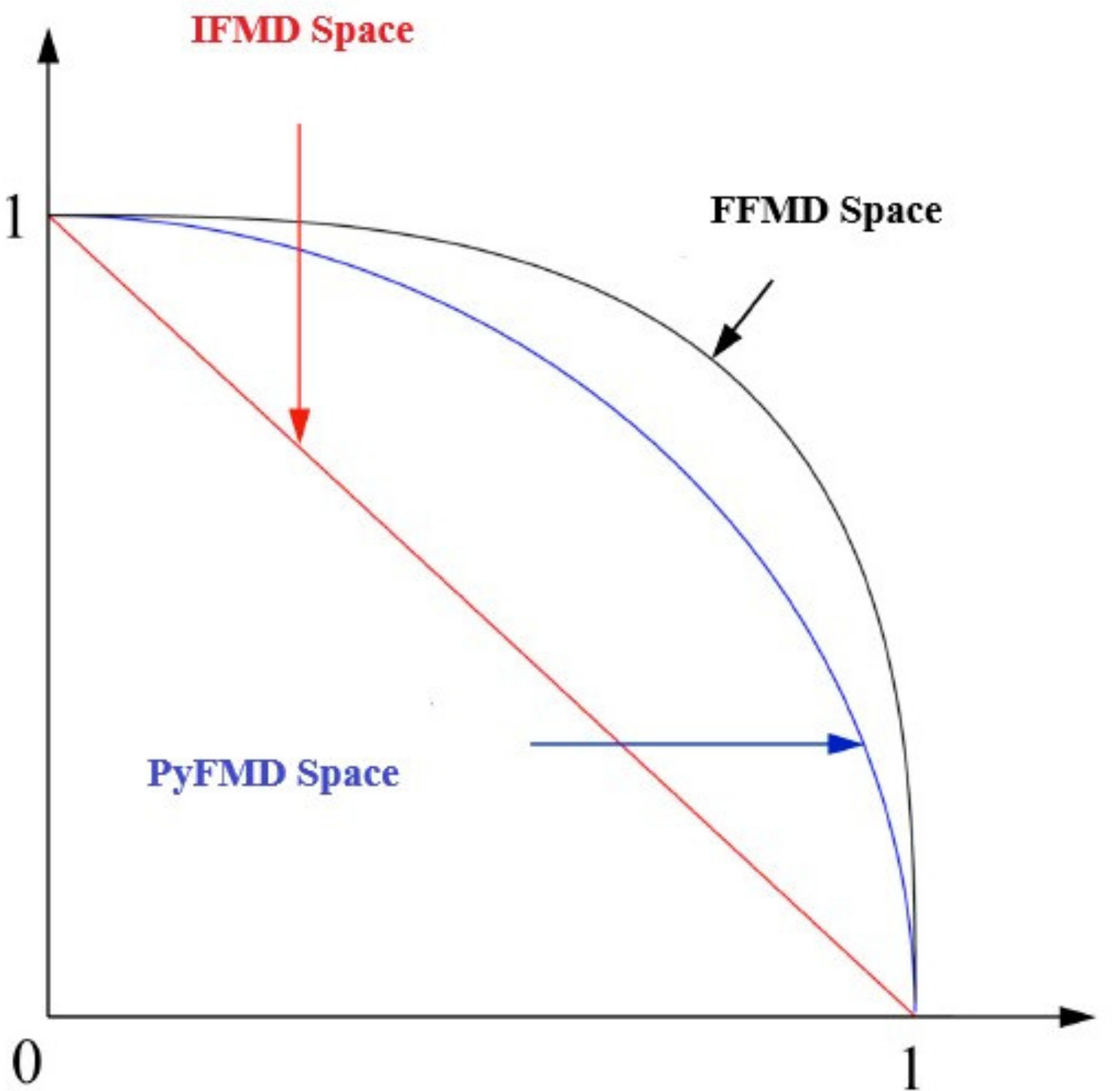
Pamucar et al. [28] obtained better results by using FUCOM to solve a given problem. Although there are several methods for prioritizing and determining the criteria weights, such as LBWA (level based weight assessment) that is used in many studies (for instance, [29]), the FUCOM algorithm provides more stable results, as it is based on multi-objective optimization. The entropy method is also a widely used method to derive criteria weights for MCDM problems (e.g., [30]). However, in our research, a significant amount of imprecision is involved. Therefore, to reduce likelihood of subjective bias, we selected the FUCOM method in the fuzzy domain. - The selection of smartphone brands is a complex decision-making problem, involving multiple criteria that are conflicting in nature. Furthermore, customer choice changes dynamically based on their preferences, demographic factors, and external influences. Therefore, establishing a multivariate model to frame the selection problem requires the consideration of the dynamics of discrete variables of the complex mechanism. Hence, the decision-making problem is associated with a substantial amount of imprecision and uncertainty. In view of this fact, we carry out our analysis using the FFS-based MCDM framework, which is capable of providing rational and robust solutions.
1.2. Contributions of the Research
- The extension of FUCOM and CODAS methods using FFS, where we apply the improved generalized score function (IGSF) as a measure for calculating score values.
- A novel hybrid FF-based combination of FUCOM and CODAS for MAGDM.
- The holistic evaluation of smartphone brands from users’ perspectives, grounded on the theoretical foundation of the UTAUT2 model.
1.3. Paper Organization
2. Related Work
2.1. Smartphone Selection
2.2. Related Work on FFS
2.3. Related Work on CODAS
2.4. Related Work on FUCOM
3. Materials and Methods
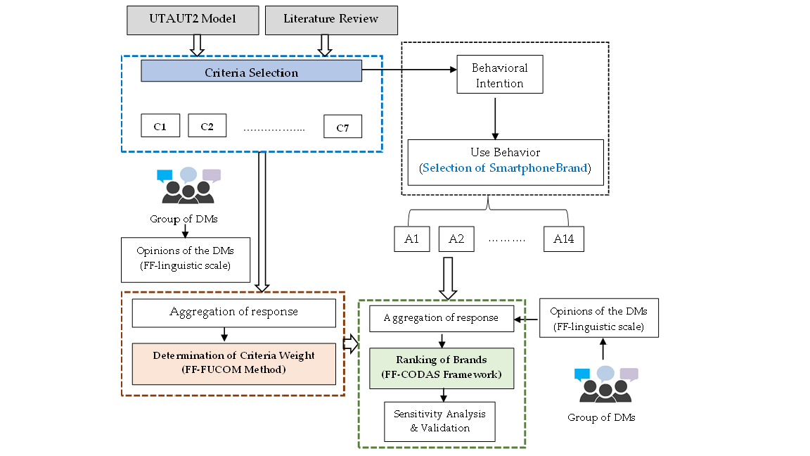
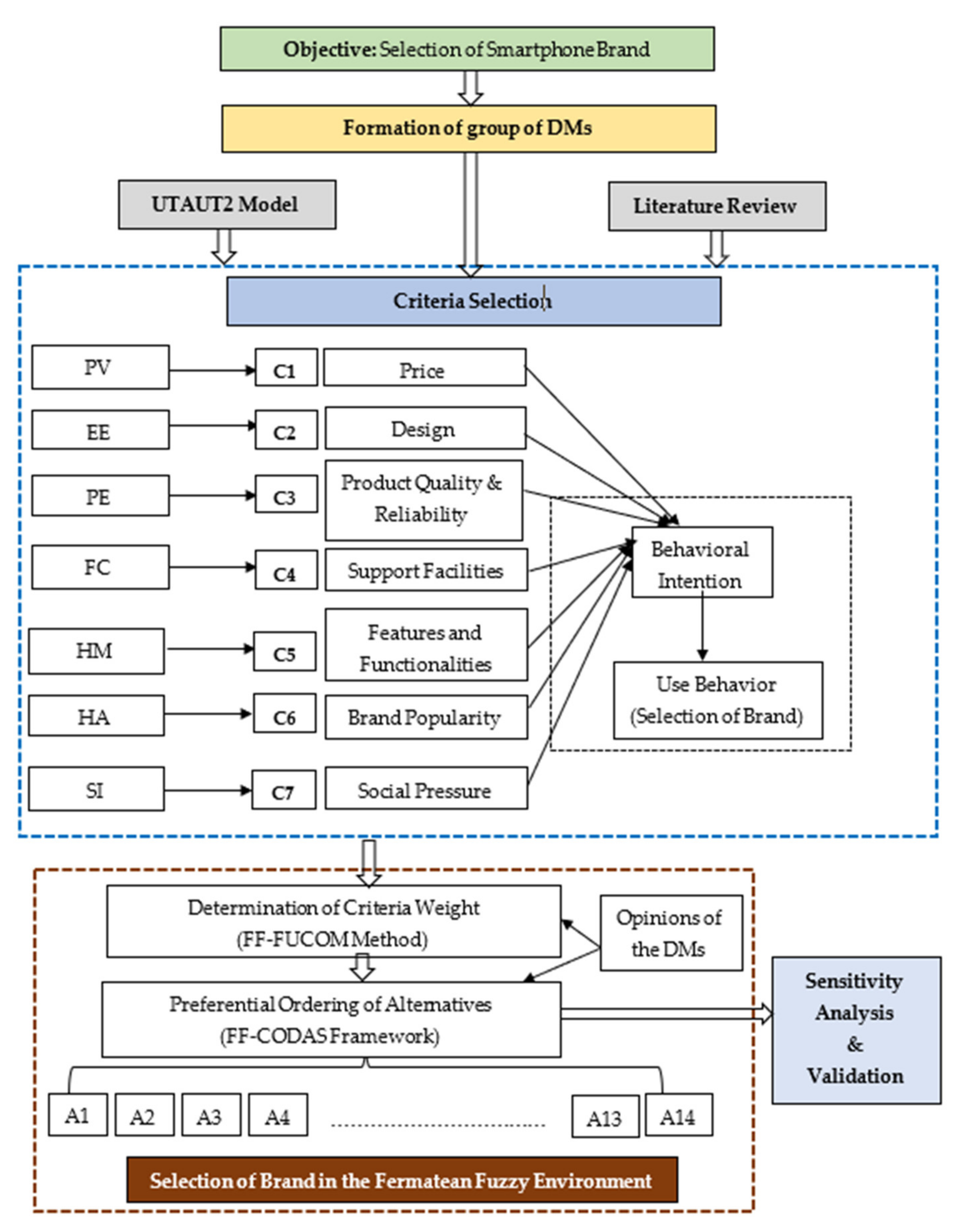
3.1. Criteria Selection
3.2. Preliminaries of FFS
3.3. FUCOM Algorithm
3.4. CODAS Algorithm
3.5. Proposed FF–FUCOM–CODAS Methodology
4. Results
5. Validation and Sensitivity Analysis
- (i)
- (ii)
- The exchange of criteria weights (e.g., [122]).
6. Research Implications
7. Conclusions and Future Scope
Author Contributions
Funding
Institutional Review Board Statement
Informed Consent Statement
Data Availability Statement
Acknowledgments
Conflicts of Interest
Declaration
Appendix A

| Decision Maker | C1 | |||||||||||||||||||||||||||
|---|---|---|---|---|---|---|---|---|---|---|---|---|---|---|---|---|---|---|---|---|---|---|---|---|---|---|---|---|
| B1 | B2 | B3 | B4 | B5 | B6 | B7 | B8 | B9 | B10 | B11 | B12 | B13 | B14 | |||||||||||||||
| DM1 | 0.6 | 0.3 | 0.5 | 0.4 | 0.8 | 0.1 | 0.9 | 0.1 | 0.6 | 0.3 | 0.6 | 0.3 | 0.6 | 0.3 | 0.5 | 0.4 | 0.5 | 0.4 | 0.5 | 0.4 | 0.6 | 0.3 | 0.5 | 0.4 | 0.5 | 0.4 | 0.6 | 0.3 |
| DM2 | 0.3 | 0.6 | 0.5 | 0.4 | 0.9 | 0.1 | 0.9 | 0.1 | 0.1 | 0.8 | 0.1 | 0.8 | 0.1 | 0.8 | 0.4 | 0.5 | 0.7 | 0.2 | 0.7 | 0.2 | 0.7 | 0.2 | 0.1 | 0.8 | 0.5 | 0.4 | 0.7 | 0.2 |
| DM3 | 0.8 | 0.1 | 0.7 | 0.2 | 0.7 | 0.2 | 0.9 | 0.1 | 0.8 | 0.1 | 0.7 | 0.2 | 0.6 | 0.3 | 0.6 | 0.3 | 0.8 | 0.1 | 0.9 | 0.1 | 0.6 | 0.3 | 0.8 | 0.1 | 0.8 | 0.1 | 0.8 | 0.1 |
| DM4 | 0.7 | 0.2 | 0.5 | 0.4 | 0.8 | 0.1 | 0.9 | 0.1 | 0.7 | 0.2 | 0.6 | 0.3 | 0.3 | 0.6 | 0.1 | 0.8 | 0.3 | 0.6 | 0.1 | 0.8 | 0.1 | 0.8 | 0.4 | 0.5 | 0.4 | 0.5 | 0.7 | 0.2 |
| DM5 | 0.7 | 0.2 | 0.7 | 0.2 | 0.8 | 0.1 | 0.9 | 0.1 | 0.6 | 0.3 | 0.7 | 0.2 | 0.6 | 0.3 | 0.6 | 0.3 | 0.5 | 0.4 | 0.6 | 0.3 | 0.7 | 0.2 | 0.4 | 0.5 | 0.7 | 0.2 | 0.6 | 0.3 |
| DM6 | 0.8 | 0.1 | 0.1 | 0.9 | 0.9 | 0.1 | 0.9 | 0.1 | 0.9 | 0.1 | 0.7 | 0.2 | 0.5 | 0.4 | 0.5 | 0.4 | 0.4 | 0.5 | 0.4 | 0.5 | 0.4 | 0.5 | 0.1 | 0.8 | 0.1 | 0.8 | 0.6 | 0.3 |
| DM7 | 0.7 | 0.2 | 0.7 | 0.2 | 0.6 | 0.3 | 0.6 | 0.3 | 0.4 | 0.5 | 0.4 | 0.5 | 0.3 | 0.6 | 0.3 | 0.6 | 0.1 | 0.8 | 0.5 | 0.4 | 0.1 | 0.8 | 0.1 | 0.8 | 0.1 | 0.8 | 0.7 | 0.2 |
| DM8 | 0.7 | 0.2 | 0.6 | 0.3 | 0.8 | 0.1 | 0.9 | 0.1 | 0.6 | 0.3 | 0.7 | 0.2 | 0.6 | 0.3 | 0.5 | 0.4 | 0.6 | 0.3 | 0.6 | 0.3 | 0.7 | 0.2 | 0.4 | 0.5 | 0.7 | 0.2 | 0.5 | 0.4 |
| DM9 | 0.8 | 0.1 | 0.9 | 0.1 | 0.9 | 0.1 | 0.9 | 0.1 | 0.7 | 0.2 | 0.7 | 0.2 | 0.6 | 0.3 | 0.8 | 0.1 | 0.7 | 0.2 | 0.6 | 0.3 | 0.5 | 0.4 | 0.3 | 0.6 | 0.1 | 0.8 | 0.1 | 0.8 |
| DM10 | 0.9 | 0.1 | 0.8 | 0.1 | 0.4 | 0.5 | 0.6 | 0.3 | 0.8 | 0.1 | 0.8 | 0.1 | 0.3 | 0.6 | 0.3 | 0.6 | 0.4 | 0.5 | 0.8 | 0.1 | 0.3 | 0.6 | 0.1 | 0.8 | 0.4 | 0.5 | 0.6 | 0.3 |
| DM11 | 0.8 | 0.1 | 0.7 | 0.2 | 0.6 | 0.3 | 0.6 | 0.3 | 0.6 | 0.3 | 0.6 | 0.3 | 0.5 | 0.4 | 0.4 | 0.5 | 0.3 | 0.6 | 0.5 | 0.4 | 0.3 | 0.6 | 0.3 | 0.6 | 0.4 | 0.5 | 0.6 | 0.3 |
| DM12 | 0.6 | 0.3 | 0.6 | 0.3 | 0.6 | 0.3 | 0.8 | 0.1 | 0.7 | 0.2 | 0.7 | 0.2 | 0.7 | 0.2 | 0.6 | 0.3 | 0.7 | 0.2 | 0.6 | 0.3 | 0.6 | 0.3 | 0.6 | 0.3 | 0.6 | 0.3 | 0.6 | 0.3 |
| DM13 | 0.4 | 0.5 | 0.4 | 0.5 | 0.4 | 0.5 | 0.4 | 0.5 | 0.4 | 0.5 | 0.4 | 0.5 | 0.4 | 0.5 | 0.4 | 0.5 | 0.4 | 0.5 | 0.4 | 0.5 | 0.4 | 0.5 | 0.4 | 0.5 | 0.4 | 0.5 | 0.4 | 0.5 |
| DM14 | 0.6 | 0.3 | 0.5 | 0.4 | 0.8 | 0.1 | 0.9 | 0.1 | 0.5 | 0.4 | 0.6 | 0.3 | 0.5 | 0.4 | 0.5 | 0.4 | 0.4 | 0.5 | 0.4 | 0.5 | 0.7 | 0.2 | 0.4 | 0.5 | 0.7 | 0.2 | 0.7 | 0.2 |
| DM15 | 0.8 | 0.1 | 0.6 | 0.3 | 0.7 | 0.2 | 0.9 | 0.1 | 0.7 | 0.2 | 0.7 | 0.2 | 0.6 | 0.3 | 0.5 | 0.4 | 0.7 | 0.2 | 0.7 | 0.2 | 0.8 | 0.1 | 0.5 | 0.4 | 0.7 | 0.2 | 0.5 | 0.4 |
| Decision Maker | C2 | |||||||||||||||||||||||||||
|---|---|---|---|---|---|---|---|---|---|---|---|---|---|---|---|---|---|---|---|---|---|---|---|---|---|---|---|---|
| B1 | B2 | B3 | B4 | B5 | B6 | B7 | B8 | B9 | B10 | B11 | B12 | B13 | B14 | |||||||||||||||
| DM1 | 0.6 | 0.3 | 0.6 | 0.3 | 0.8 | 0.1 | 0.8 | 0.1 | 0.8 | 0.1 | 0.8 | 0.1 | 0.6 | 0.3 | 0.6 | 0.3 | 0.6 | 0.3 | 0.5 | 0.4 | 0.6 | 0.3 | 0.4 | 0.5 | 0.5 | 0.4 | 0.6 | 0.3 |
| DM2 | 0.5 | 0.4 | 0.5 | 0.4 | 0.9 | 0.1 | 0.9 | 0.1 | 0.4 | 0.5 | 0.4 | 0.5 | 0.4 | 0.5 | 0.4 | 0.5 | 0.7 | 0.2 | 0.7 | 0.2 | 0.7 | 0.2 | 0.4 | 0.5 | 0.7 | 0.2 | 0.7 | 0.2 |
| DM3 | 0.7 | 0.2 | 0.7 | 0.2 | 0.7 | 0.2 | 0.9 | 0.1 | 0.8 | 0.1 | 0.7 | 0.2 | 0.7 | 0.2 | 0.7 | 0.2 | 0.8 | 0.1 | 0.8 | 0.1 | 0.7 | 0.2 | 0.7 | 0.2 | 0.7 | 0.2 | 0.8 | 0.1 |
| DM4 | 0.7 | 0.2 | 0.7 | 0.2 | 0.9 | 0.1 | 0.9 | 0.1 | 0.7 | 0.2 | 0.8 | 0.1 | 0.7 | 0.2 | 0.5 | 0.4 | 0.5 | 0.4 | 0.5 | 0.4 | 0.5 | 0.4 | 0.5 | 0.4 | 0.5 | 0.4 | 0.5 | 0.4 |
| DM5 | 0.6 | 0.3 | 0.7 | 0.2 | 0.8 | 0.1 | 0.9 | 0.1 | 0.7 | 0.2 | 0.7 | 0.2 | 0.6 | 0.3 | 0.6 | 0.3 | 0.5 | 0.4 | 0.7 | 0.2 | 0.7 | 0.2 | 0.5 | 0.4 | 0.8 | 0.1 | 0.7 | 0.2 |
| DM6 | 0.8 | 0.1 | 0.4 | 0.5 | 0.9 | 0.1 | 0.9 | 0.1 | 0.9 | 0.1 | 0.7 | 0.2 | 0.1 | 0.8 | 0.1 | 0.8 | 0.1 | 0.9 | 0.1 | 0.8 | 0.1 | 0.8 | 0.1 | 0.8 | 0.1 | 0.9 | 0.5 | 0.4 |
| DM7 | 0.8 | 0.1 | 0.7 | 0.2 | 0.7 | 0.2 | 0.7 | 0.2 | 0.4 | 0.5 | 0.4 | 0.5 | 0.4 | 0.5 | 0.4 | 0.5 | 0.4 | 0.5 | 0.4 | 0.5 | 0.4 | 0.5 | 0.4 | 0.5 | 0.5 | 0.4 | 0.7 | 0.2 |
| DM8 | 0.8 | 0.1 | 0.7 | 0.2 | 0.8 | 0.1 | 0.9 | 0.1 | 0.7 | 0.2 | 0.8 | 0.1 | 0.6 | 0.3 | 0.6 | 0.3 | 0.7 | 0.2 | 0.7 | 0.2 | 0.7 | 0.2 | 0.4 | 0.5 | 0.8 | 0.1 | 0.8 | 0.1 |
| DM9 | 0.8 | 0.1 | 0.9 | 0.1 | 0.9 | 0.1 | 0.9 | 0.1 | 0.7 | 0.2 | 0.7 | 0.2 | 0.6 | 0.3 | 0.8 | 0.1 | 0.5 | 0.4 | 0.1 | 0.8 | 0.1 | 0.9 | 0.1 | 0.9 | 0.1 | 0.9 | 0.8 | 0.1 |
| DM10 | 0.9 | 0.1 | 0.8 | 0.1 | 0.5 | 0.4 | 0.8 | 0.1 | 0.8 | 0.1 | 0.8 | 0.1 | 0.3 | 0.6 | 0.5 | 0.4 | 0.4 | 0.5 | 0.7 | 0.2 | 0.7 | 0.2 | 0.3 | 0.6 | 0.4 | 0.5 | 0.8 | 0.1 |
| DM11 | 0.9 | 0.1 | 0.7 | 0.2 | 0.9 | 0.1 | 0.9 | 0.1 | 0.6 | 0.3 | 0.6 | 0.3 | 0.6 | 0.3 | 0.7 | 0.2 | 0.5 | 0.4 | 0.7 | 0.2 | 0.5 | 0.4 | 0.3 | 0.6 | 0.3 | 0.6 | 0.5 | 0.4 |
| DM12 | 0.7 | 0.2 | 0.6 | 0.3 | 0.6 | 0.3 | 0.8 | 0.1 | 0.7 | 0.2 | 0.7 | 0.2 | 0.7 | 0.2 | 0.6 | 0.3 | 0.7 | 0.2 | 0.6 | 0.3 | 0.6 | 0.3 | 0.6 | 0.3 | 0.6 | 0.3 | 0.7 | 0.2 |
| DM13 | 0.6 | 0.3 | 0.6 | 0.3 | 0.6 | 0.3 | 0.6 | 0.3 | 0.6 | 0.3 | 0.6 | 0.3 | 0.6 | 0.3 | 0.6 | 0.3 | 0.6 | 0.3 | 0.6 | 0.3 | 0.6 | 0.3 | 0.6 | 0.3 | 0.6 | 0.3 | 0.6 | 0.3 |
| DM14 | 0.6 | 0.3 | 0.6 | 0.3 | 0.9 | 0.1 | 0.7 | 0.2 | 0.6 | 0.3 | 0.7 | 0.2 | 0.8 | 0.1 | 0.6 | 0.3 | 0.5 | 0.4 | 0.4 | 0.5 | 0.7 | 0.2 | 0.8 | 0.1 | 0.7 | 0.2 | 0.8 | 0.1 |
| DM15 | 0.9 | 0.1 | 0.8 | 0.1 | 0.8 | 0.1 | 0.9 | 0.1 | 0.9 | 0.1 | 0.8 | 0.1 | 0.7 | 0.2 | 0.7 | 0.2 | 0.8 | 0.1 | 0.7 | 0.2 | 0.6 | 0.3 | 0.6 | 0.3 | 0.7 | 0.2 | 0.7 | 0.2 |
| Decision Maker | C3 | |||||||||||||||||||||||||||
|---|---|---|---|---|---|---|---|---|---|---|---|---|---|---|---|---|---|---|---|---|---|---|---|---|---|---|---|---|
| B1 | B2 | B3 | B4 | B5 | B6 | B7 | B8 | B9 | B10 | B11 | B12 | B13 | B14 | |||||||||||||||
| DM1 | 0.7 | 0.2 | 0.6 | 0.3 | 0.7 | 0.2 | 0.7 | 0.2 | 0.8 | 0.1 | 0.8 | 0.1 | 0.6 | 0.3 | 0.6 | 0.3 | 0.6 | 0.3 | 0.6 | 0.3 | 0.6 | 0.3 | 0.6 | 0.3 | 0.7 | 0.2 | 0.7 | 0.2 |
| DM2 | 0.7 | 0.2 | 0.7 | 0.2 | 0.9 | 0.1 | 0.9 | 0.1 | 0.6 | 0.3 | 0.6 | 0.3 | 0.5 | 0.4 | 0.6 | 0.3 | 0.8 | 0.1 | 0.7 | 0.2 | 0.8 | 0.1 | 0.5 | 0.4 | 0.7 | 0.2 | 0.8 | 0.1 |
| DM3 | 0.7 | 0.2 | 0.7 | 0.2 | 0.7 | 0.2 | 0.9 | 0.1 | 0.7 | 0.2 | 0.7 | 0.2 | 0.7 | 0.2 | 0.7 | 0.2 | 0.8 | 0.1 | 0.8 | 0.1 | 0.7 | 0.2 | 0.7 | 0.2 | 0.7 | 0.2 | 0.7 | 0.2 |
| DM4 | 0.6 | 0.3 | 0.5 | 0.4 | 0.8 | 0.1 | 0.9 | 0.1 | 0.8 | 0.1 | 0.8 | 0.1 | 0.6 | 0.3 | 0.6 | 0.3 | 0.4 | 0.5 | 0.4 | 0.5 | 0.3 | 0.6 | 0.5 | 0.4 | 0.4 | 0.5 | 0.6 | 0.3 |
| DM5 | 0.7 | 0.2 | 0.7 | 0.2 | 0.8 | 0.1 | 0.9 | 0.1 | 0.7 | 0.2 | 0.7 | 0.2 | 0.6 | 0.3 | 0.6 | 0.3 | 0.6 | 0.3 | 0.6 | 0.3 | 0.7 | 0.2 | 0.5 | 0.4 | 0.8 | 0.1 | 0.7 | 0.2 |
| DM6 | 0.8 | 0.1 | 0.6 | 0.3 | 0.9 | 0.1 | 0.9 | 0.1 | 0.8 | 0.1 | 0.8 | 0.1 | 0.1 | 0.8 | 0.1 | 0.8 | 0.1 | 0.8 | 0.1 | 0.9 | 0.1 | 0.9 | 0.1 | 0.9 | 0.1 | 0.9 | 0.7 | 0.2 |
| DM7 | 0.8 | 0.1 | 0.8 | 0.1 | 0.8 | 0.1 | 0.8 | 0.1 | 0.6 | 0.3 | 0.5 | 0.4 | 0.4 | 0.5 | 0.4 | 0.5 | 0.4 | 0.5 | 0.4 | 0.5 | 0.4 | 0.5 | 0.4 | 0.5 | 0.4 | 0.5 | 0.6 | 0.3 |
| DM8 | 0.8 | 0.1 | 0.7 | 0.2 | 0.8 | 0.1 | 0.9 | 0.1 | 0.7 | 0.2 | 0.8 | 0.1 | 0.7 | 0.2 | 0.7 | 0.2 | 0.6 | 0.3 | 0.6 | 0.3 | 0.7 | 0.2 | 0.5 | 0.4 | 0.7 | 0.2 | 0.7 | 0.2 |
| DM9 | 0.8 | 0.1 | 0.9 | 0.1 | 0.9 | 0.1 | 0.9 | 0.1 | 0.4 | 0.5 | 0.3 | 0.6 | 0.6 | 0.3 | 0.8 | 0.1 | 0.6 | 0.3 | 0.6 | 0.3 | 0.1 | 0.9 | 0.1 | 0.9 | 0.1 | 0.9 | 0.8 | 0.1 |
| DM10 | 0.8 | 0.1 | 0.8 | 0.1 | 0.6 | 0.3 | 0.9 | 0.1 | 0.8 | 0.1 | 0.8 | 0.1 | 0.3 | 0.6 | 0.5 | 0.4 | 0.3 | 0.6 | 0.7 | 0.2 | 0.3 | 0.6 | 0.1 | 0.8 | 0.4 | 0.5 | 0.8 | 0.1 |
| DM11 | 0.9 | 0.1 | 0.7 | 0.2 | 0.9 | 0.1 | 0.9 | 0.1 | 0.5 | 0.4 | 0.5 | 0.4 | 0.5 | 0.4 | 0.6 | 0.3 | 0.4 | 0.5 | 0.7 | 0.2 | 0.6 | 0.3 | 0.3 | 0.6 | 0.3 | 0.6 | 0.5 | 0.4 |
| DM12 | 0.7 | 0.2 | 0.6 | 0.3 | 0.6 | 0.3 | 0.7 | 0.2 | 0.7 | 0.2 | 0.7 | 0.2 | 0.6 | 0.3 | 0.6 | 0.3 | 0.7 | 0.2 | 0.6 | 0.3 | 0.6 | 0.3 | 0.6 | 0.3 | 0.6 | 0.3 | 0.7 | 0.2 |
| DM13 | 0.6 | 0.3 | 0.6 | 0.3 | 0.6 | 0.3 | 0.6 | 0.3 | 0.6 | 0.3 | 0.6 | 0.3 | 0.6 | 0.3 | 0.6 | 0.3 | 0.6 | 0.3 | 0.6 | 0.3 | 0.6 | 0.3 | 0.6 | 0.3 | 0.6 | 0.3 | 0.6 | 0.3 |
| DM14 | 0.7 | 0.2 | 0.7 | 0.2 | 0.9 | 0.1 | 0.9 | 0.1 | 0.5 | 0.4 | 0.6 | 0.3 | 0.7 | 0.2 | 0.5 | 0.4 | 0.3 | 0.6 | 0.6 | 0.3 | 0.6 | 0.3 | 0.4 | 0.5 | 0.5 | 0.4 | 0.6 | 0.3 |
| DM15 | 0.9 | 0.1 | 0.8 | 0.1 | 0.8 | 0.1 | 0.9 | 0.1 | 0.7 | 0.2 | 0.7 | 0.2 | 0.6 | 0.3 | 0.6 | 0.3 | 0.7 | 0.2 | 0.7 | 0.2 | 0.6 | 0.3 | 0.5 | 0.4 | 0.7 | 0.2 | 0.7 | 0.2 |
| Decision Maker | C4 | |||||||||||||||||||||||||||
|---|---|---|---|---|---|---|---|---|---|---|---|---|---|---|---|---|---|---|---|---|---|---|---|---|---|---|---|---|
| B1 | B2 | B3 | B4 | B5 | B6 | B7 | B8 | B9 | B10 | B11 | B12 | B13 | B14 | |||||||||||||||
| DM1 | 0.6 | 0.3 | 0.5 | 0.4 | 0.6 | 0.3 | 0.7 | 0.2 | 0.7 | 0.2 | 0.7 | 0.2 | 0.5 | 0.4 | 0.5 | 0.4 | 0.5 | 0.4 | 0.8 | 0.1 | 0.7 | 0.2 | 0.5 | 0.4 | 0.5 | 0.4 | 0.6 | 0.3 |
| DM2 | 0.7 | 0.2 | 0.7 | 0.2 | 0.9 | 0.1 | 0.9 | 0.1 | 0.6 | 0.3 | 0.6 | 0.3 | 0.6 | 0.3 | 0.6 | 0.3 | 0.6 | 0.3 | 0.6 | 0.3 | 0.7 | 0.2 | 0.5 | 0.4 | 0.6 | 0.3 | 0.8 | 0.1 |
| DM3 | 0.7 | 0.2 | 0.7 | 0.2 | 0.7 | 0.2 | 0.9 | 0.1 | 0.7 | 0.2 | 0.7 | 0.2 | 0.7 | 0.2 | 0.7 | 0.2 | 0.7 | 0.2 | 0.8 | 0.1 | 0.7 | 0.2 | 0.7 | 0.2 | 0.7 | 0.2 | 0.7 | 0.2 |
| DM4 | 0.5 | 0.4 | 0.5 | 0.4 | 0.7 | 0.2 | 0.8 | 0.1 | 0.7 | 0.2 | 0.6 | 0.3 | 0.5 | 0.4 | 0.4 | 0.5 | 0.4 | 0.5 | 0.3 | 0.6 | 0.1 | 0.8 | 0.5 | 0.4 | 0.3 | 0.6 | 0.7 | 0.2 |
| DM5 | 0.6 | 0.3 | 0.6 | 0.3 | 0.8 | 0.1 | 0.9 | 0.1 | 0.6 | 0.3 | 0.7 | 0.2 | 0.6 | 0.3 | 0.6 | 0.3 | 0.6 | 0.3 | 0.7 | 0.2 | 0.7 | 0.2 | 0.5 | 0.4 | 0.7 | 0.2 | 0.7 | 0.2 |
| DM6 | 0.9 | 0.1 | 0.5 | 0.4 | 0.9 | 0.1 | 0.9 | 0.1 | 0.9 | 0.1 | 0.7 | 0.2 | 0.8 | 0.1 | 0.6 | 0.3 | 0.5 | 0.4 | 0.7 | 0.2 | 0.4 | 0.5 | 0.5 | 0.4 | 0.1 | 0.8 | 0.6 | 0.3 |
| DM7 | 0.8 | 0.1 | 0.8 | 0.1 | 0.8 | 0.1 | 0.7 | 0.2 | 0.5 | 0.4 | 0.5 | 0.4 | 0.4 | 0.5 | 0.3 | 0.6 | 0.6 | 0.3 | 0.3 | 0.6 | 0.3 | 0.6 | 0.3 | 0.6 | 0.3 | 0.6 | 0.3 | 0.6 |
| DM8 | 0.7 | 0.2 | 0.6 | 0.3 | 0.8 | 0.1 | 0.8 | 0.1 | 0.7 | 0.2 | 0.7 | 0.2 | 0.7 | 0.2 | 0.6 | 0.3 | 0.6 | 0.3 | 0.6 | 0.3 | 0.6 | 0.3 | 0.6 | 0.3 | 0.7 | 0.2 | 0.7 | 0.2 |
| DM9 | 0.8 | 0.1 | 0.9 | 0.1 | 0.9 | 0.1 | 0.9 | 0.1 | 0.7 | 0.2 | 0.5 | 0.4 | 0.4 | 0.5 | 0.7 | 0.2 | 0.1 | 0.8 | 0.1 | 0.8 | 0.1 | 0.9 | 0.1 | 0.9 | 0.1 | 0.9 | 0.8 | 0.1 |
| DM10 | 0.8 | 0.1 | 0.8 | 0.1 | 0.7 | 0.2 | 0.9 | 0.1 | 0.8 | 0.1 | 0.8 | 0.1 | 0.3 | 0.6 | 0.4 | 0.5 | 0.3 | 0.6 | 0.7 | 0.2 | 0.1 | 0.8 | 0.1 | 0.9 | 0.3 | 0.6 | 0.8 | 0.1 |
| DM11 | 0.8 | 0.1 | 0.7 | 0.2 | 0.8 | 0.1 | 0.9 | 0.1 | 0.5 | 0.4 | 0.5 | 0.4 | 0.5 | 0.4 | 0.5 | 0.4 | 0.5 | 0.4 | 0.6 | 0.3 | 0.6 | 0.3 | 0.5 | 0.4 | 0.5 | 0.4 | 0.5 | 0.4 |
| DM12 | 0.7 | 0.2 | 0.7 | 0.2 | 0.6 | 0.3 | 0.7 | 0.2 | 0.7 | 0.2 | 0.7 | 0.2 | 0.6 | 0.3 | 0.6 | 0.3 | 0.7 | 0.2 | 0.6 | 0.3 | 0.6 | 0.3 | 0.6 | 0.3 | 0.6 | 0.3 | 0.7 | 0.2 |
| DM13 | 0.6 | 0.3 | 0.6 | 0.3 | 0.6 | 0.3 | 0.6 | 0.3 | 0.6 | 0.3 | 0.6 | 0.3 | 0.6 | 0.3 | 0.6 | 0.3 | 0.6 | 0.3 | 0.6 | 0.3 | 0.6 | 0.3 | 0.6 | 0.3 | 0.6 | 0.3 | 0.6 | 0.3 |
| DM14 | 0.9 | 0.1 | 0.8 | 0.1 | 0.7 | 0.2 | 0.7 | 0.2 | 0.4 | 0.5 | 0.5 | 0.4 | 0.5 | 0.4 | 0.3 | 0.6 | 0.3 | 0.6 | 0.5 | 0.4 | 0.3 | 0.6 | 0.4 | 0.5 | 0.1 | 0.8 | 0.5 | 0.4 |
| DM15 | 0.8 | 0.1 | 0.9 | 0.1 | 0.9 | 0.1 | 0.8 | 0.1 | 0.7 | 0.2 | 0.7 | 0.2 | 0.6 | 0.3 | 0.6 | 0.3 | 0.7 | 0.2 | 0.8 | 0.1 | 0.7 | 0.2 | 0.5 | 0.4 | 0.7 | 0.2 | 0.7 | 0.2 |
| Decision Maker | C5 | |||||||||||||||||||||||||||
|---|---|---|---|---|---|---|---|---|---|---|---|---|---|---|---|---|---|---|---|---|---|---|---|---|---|---|---|---|
| B1 | B2 | B3 | B4 | B5 | B6 | B7 | B8 | B9 | B10 | B11 | B12 | B13 | B14 | |||||||||||||||
| DM1 | 0.7 | 0.2 | 0.5 | 0.4 | 0.7 | 0.2 | 0.7 | 0.2 | 0.8 | 0.1 | 0.8 | 0.1 | 0.6 | 0.3 | 0.6 | 0.3 | 0.6 | 0.3 | 0.8 | 0.1 | 0.7 | 0.2 | 0.6 | 0.3 | 0.7 | 0.2 | 0.7 | 0.2 |
| DM2 | 0.7 | 0.2 | 0.7 | 0.2 | 0.9 | 0.1 | 0.9 | 0.1 | 0.6 | 0.3 | 0.7 | 0.2 | 0.6 | 0.3 | 0.6 | 0.3 | 0.8 | 0.1 | 0.8 | 0.1 | 0.8 | 0.1 | 0.6 | 0.3 | 0.8 | 0.1 | 0.8 | 0.1 |
| DM3 | 0.7 | 0.2 | 0.7 | 0.2 | 0.7 | 0.2 | 0.9 | 0.1 | 0.7 | 0.2 | 0.7 | 0.2 | 0.7 | 0.2 | 0.7 | 0.2 | 0.7 | 0.2 | 0.7 | 0.2 | 0.7 | 0.2 | 0.7 | 0.2 | 0.7 | 0.2 | 0.7 | 0.2 |
| DM4 | 0.7 | 0.2 | 0.7 | 0.2 | 0.8 | 0.1 | 0.8 | 0.1 | 0.8 | 0.1 | 0.6 | 0.3 | 0.5 | 0.4 | 0.4 | 0.5 | 0.5 | 0.4 | 0.5 | 0.4 | 0.5 | 0.4 | 0.6 | 0.3 | 0.4 | 0.5 | 0.7 | 0.2 |
| DM5 | 0.6 | 0.3 | 0.6 | 0.3 | 0.8 | 0.1 | 0.9 | 0.1 | 0.7 | 0.2 | 0.7 | 0.2 | 0.6 | 0.3 | 0.6 | 0.3 | 0.6 | 0.3 | 0.6 | 0.3 | 0.7 | 0.2 | 0.5 | 0.4 | 0.8 | 0.1 | 0.7 | 0.2 |
| DM6 | 0.8 | 0.1 | 0.7 | 0.2 | 0.9 | 0.1 | 0.9 | 0.1 | 0.9 | 0.1 | 0.9 | 0.1 | 0.1 | 0.9 | 0.1 | 0.9 | 0.1 | 0.9 | 0.1 | 0.9 | 0.1 | 0.9 | 0.1 | 0.9 | 0.1 | 0.9 | 0.6 | 0.3 |
| DM7 | 0.8 | 0.1 | 0.8 | 0.1 | 0.8 | 0.1 | 0.7 | 0.2 | 0.5 | 0.4 | 0.4 | 0.5 | 0.4 | 0.5 | 0.4 | 0.5 | 0.4 | 0.5 | 0.4 | 0.5 | 0.4 | 0.5 | 0.4 | 0.5 | 0.4 | 0.5 | 0.4 | 0.5 |
| DM8 | 0.8 | 0.1 | 0.8 | 0.1 | 0.9 | 0.1 | 0.9 | 0.1 | 0.8 | 0.1 | 0.8 | 0.1 | 0.8 | 0.1 | 0.8 | 0.1 | 0.7 | 0.2 | 0.8 | 0.1 | 0.7 | 0.2 | 0.7 | 0.2 | 0.8 | 0.1 | 0.8 | 0.1 |
| DM9 | 0.8 | 0.1 | 0.9 | 0.1 | 0.9 | 0.1 | 0.9 | 0.1 | 0.6 | 0.3 | 0.6 | 0.3 | 0.6 | 0.3 | 0.8 | 0.1 | 0.7 | 0.2 | 0.7 | 0.2 | 0.3 | 0.6 | 0.3 | 0.6 | 0.3 | 0.6 | 0.8 | 0.1 |
| DM10 | 0.9 | 0.1 | 0.9 | 0.1 | 0.8 | 0.1 | 0.8 | 0.1 | 0.9 | 0.1 | 0.9 | 0.1 | 0.3 | 0.6 | 0.6 | 0.3 | 0.3 | 0.6 | 0.7 | 0.2 | 0.1 | 0.8 | 0.1 | 0.9 | 0.5 | 0.4 | 0.8 | 0.1 |
| DM11 | 0.7 | 0.2 | 0.6 | 0.3 | 0.8 | 0.1 | 0.8 | 0.1 | 0.4 | 0.5 | 0.4 | 0.5 | 0.4 | 0.5 | 0.5 | 0.4 | 0.5 | 0.4 | 0.5 | 0.4 | 0.4 | 0.5 | 0.4 | 0.5 | 0.4 | 0.5 | 0.6 | 0.3 |
| DM12 | 0.7 | 0.2 | 0.6 | 0.3 | 0.6 | 0.3 | 0.7 | 0.2 | 0.7 | 0.2 | 0.7 | 0.2 | 0.6 | 0.3 | 0.6 | 0.3 | 0.7 | 0.2 | 0.6 | 0.3 | 0.6 | 0.3 | 0.6 | 0.3 | 0.6 | 0.3 | 0.7 | 0.2 |
| DM13 | 0.6 | 0.3 | 0.6 | 0.3 | 0.6 | 0.3 | 0.6 | 0.3 | 0.6 | 0.3 | 0.6 | 0.3 | 0.6 | 0.3 | 0.6 | 0.3 | 0.6 | 0.3 | 0.6 | 0.3 | 0.6 | 0.3 | 0.6 | 0.3 | 0.6 | 0.3 | 0.6 | 0.3 |
| DM14 | 0.7 | 0.2 | 0.8 | 0.1 | 0.9 | 0.1 | 0.9 | 0.1 | 0.7 | 0.2 | 0.6 | 0.3 | 0.6 | 0.3 | 0.6 | 0.3 | 0.3 | 0.6 | 0.3 | 0.6 | 0.4 | 0.5 | 0.4 | 0.5 | 0.1 | 0.8 | 0.7 | 0.2 |
| DM15 | 0.9 | 0.1 | 0.9 | 0.1 | 0.8 | 0.1 | 0.9 | 0.1 | 0.9 | 0.1 | 0.8 | 0.1 | 0.7 | 0.2 | 0.7 | 0.2 | 0.6 | 0.3 | 0.7 | 0.2 | 0.6 | 0.3 | 0.5 | 0.4 | 0.8 | 0.1 | 0.8 | 0.1 |
| Decision Maker | C6 | |||||||||||||||||||||||||||
|---|---|---|---|---|---|---|---|---|---|---|---|---|---|---|---|---|---|---|---|---|---|---|---|---|---|---|---|---|
| B1 | B2 | B3 | B4 | B5 | B6 | B7 | B8 | B9 | B10 | B11 | B12 | B13 | B14 | |||||||||||||||
| DM1 | 0.6 | 0.3 | 0.6 | 0.3 | 0.7 | 0.2 | 0.8 | 0.1 | 0.8 | 0.1 | 0.8 | 0.1 | 0.6 | 0.3 | 0.6 | 0.3 | 0.6 | 0.3 | 0.8 | 0.1 | 0.6 | 0.3 | 0.6 | 0.3 | 0.6 | 0.3 | 0.8 | 0.1 |
| DM2 | 0.8 | 0.1 | 0.7 | 0.2 | 0.9 | 0.1 | 0.9 | 0.1 | 0.6 | 0.3 | 0.6 | 0.3 | 0.5 | 0.4 | 0.7 | 0.2 | 0.8 | 0.1 | 0.8 | 0.1 | 0.8 | 0.1 | 0.6 | 0.3 | 0.8 | 0.1 | 0.8 | 0.1 |
| DM3 | 0.8 | 0.1 | 0.6 | 0.3 | 0.7 | 0.2 | 0.9 | 0.1 | 0.7 | 0.2 | 0.8 | 0.1 | 0.8 | 0.1 | 0.8 | 0.1 | 0.8 | 0.1 | 0.8 | 0.1 | 0.7 | 0.2 | 0.8 | 0.1 | 0.8 | 0.1 | 0.8 | 0.1 |
| DM4 | 0.7 | 0.2 | 0.7 | 0.2 | 0.8 | 0.1 | 0.8 | 0.1 | 0.6 | 0.3 | 0.5 | 0.4 | 0.4 | 0.5 | 0.3 | 0.6 | 0.3 | 0.6 | 0.7 | 0.2 | 0.1 | 0.8 | 0.5 | 0.4 | 0.7 | 0.2 | 0.7 | 0.2 |
| DM5 | 0.5 | 0.4 | 0.5 | 0.4 | 0.8 | 0.1 | 0.9 | 0.1 | 0.7 | 0.2 | 0.7 | 0.2 | 0.6 | 0.3 | 0.6 | 0.3 | 0.5 | 0.4 | 0.5 | 0.4 | 0.6 | 0.3 | 0.4 | 0.5 | 0.7 | 0.2 | 0.5 | 0.4 |
| DM6 | 0.9 | 0.1 | 0.1 | 0.8 | 0.9 | 0.1 | 0.9 | 0.1 | 0.8 | 0.1 | 0.8 | 0.1 | 0.7 | 0.2 | 0.7 | 0.2 | 0.4 | 0.5 | 0.7 | 0.2 | 0.6 | 0.3 | 0.4 | 0.5 | 0.7 | 0.2 | 0.5 | 0.4 |
| DM7 | 0.8 | 0.1 | 0.8 | 0.1 | 0.8 | 0.1 | 0.7 | 0.2 | 0.5 | 0.4 | 0.5 | 0.4 | 0.5 | 0.4 | 0.5 | 0.4 | 0.5 | 0.4 | 0.4 | 0.5 | 0.4 | 0.5 | 0.4 | 0.5 | 0.4 | 0.5 | 0.5 | 0.4 |
| DM8 | 0.8 | 0.1 | 0.7 | 0.2 | 0.9 | 0.1 | 0.9 | 0.1 | 0.7 | 0.2 | 0.7 | 0.2 | 0.6 | 0.3 | 0.6 | 0.3 | 0.5 | 0.4 | 0.6 | 0.3 | 0.6 | 0.3 | 0.5 | 0.4 | 0.7 | 0.2 | 0.7 | 0.2 |
| DM9 | 0.6 | 0.3 | 0.9 | 0.1 | 0.9 | 0.1 | 0.9 | 0.1 | 0.7 | 0.2 | 0.7 | 0.2 | 0.6 | 0.3 | 0.8 | 0.1 | 0.6 | 0.3 | 0.7 | 0.2 | 0.5 | 0.4 | 0.3 | 0.6 | 0.3 | 0.6 | 0.7 | 0.2 |
| DM10 | 0.9 | 0.1 | 0.9 | 0.1 | 0.7 | 0.2 | 0.9 | 0.1 | 0.9 | 0.1 | 0.9 | 0.1 | 0.5 | 0.4 | 0.6 | 0.3 | 0.3 | 0.6 | 0.7 | 0.2 | 0.4 | 0.5 | 0.1 | 0.8 | 0.6 | 0.3 | 0.8 | 0.1 |
| DM11 | 0.9 | 0.1 | 0.8 | 0.1 | 0.9 | 0.1 | 0.9 | 0.1 | 0.6 | 0.3 | 0.6 | 0.3 | 0.6 | 0.3 | 0.6 | 0.3 | 0.4 | 0.5 | 0.6 | 0.3 | 0.6 | 0.3 | 0.4 | 0.5 | 0.4 | 0.5 | 0.6 | 0.3 |
| DM12 | 0.8 | 0.1 | 0.6 | 0.3 | 0.7 | 0.2 | 0.8 | 0.1 | 0.8 | 0.1 | 0.8 | 0.1 | 0.6 | 0.3 | 0.6 | 0.3 | 0.7 | 0.2 | 0.6 | 0.3 | 0.6 | 0.3 | 0.6 | 0.3 | 0.6 | 0.3 | 0.7 | 0.2 |
| DM13 | 0.6 | 0.3 | 0.6 | 0.3 | 0.6 | 0.3 | 0.6 | 0.3 | 0.6 | 0.3 | 0.6 | 0.3 | 0.6 | 0.3 | 0.6 | 0.3 | 0.6 | 0.3 | 0.6 | 0.3 | 0.6 | 0.3 | 0.6 | 0.3 | 0.6 | 0.3 | 0.6 | 0.3 |
| DM14 | 0.8 | 0.1 | 0.9 | 0.1 | 0.9 | 0.1 | 0.9 | 0.1 | 0.5 | 0.4 | 0.6 | 0.3 | 0.4 | 0.5 | 0.3 | 0.6 | 0.1 | 0.8 | 0.5 | 0.4 | 0.3 | 0.6 | 0.4 | 0.5 | 0.5 | 0.4 | 0.7 | 0.2 |
| DM15 | 0.8 | 0.1 | 0.9 | 0.1 | 0.8 | 0.1 | 0.9 | 0.1 | 0.8 | 0.1 | 0.8 | 0.1 | 0.6 | 0.3 | 0.6 | 0.3 | 0.7 | 0.2 | 0.6 | 0.3 | 0.6 | 0.3 | 0.4 | 0.5 | 0.7 | 0.2 | 0.8 | 0.1 |
| Decision Maker | C7 | |||||||||||||||||||||||||||
|---|---|---|---|---|---|---|---|---|---|---|---|---|---|---|---|---|---|---|---|---|---|---|---|---|---|---|---|---|
| B1 | B2 | B3 | B4 | B5 | B6 | B7 | B8 | B9 | B10 | B11 | B12 | B13 | B14 | |||||||||||||||
| DM1 | 0.7 | 0.2 | 0.6 | 0.3 | 0.7 | 0.2 | 0.9 | 0.1 | 0.8 | 0.1 | 0.8 | 0.1 | 0.6 | 0.3 | 0.6 | 0.3 | 0.6 | 0.3 | 0.7 | 0.2 | 0.7 | 0.2 | 0.6 | 0.3 | 0.6 | 0.3 | 0.8 | 0.1 |
| DM2 | 0.9 | 0.1 | 0.8 | 0.1 | 0.9 | 0.1 | 0.9 | 0.1 | 0.7 | 0.2 | 0.7 | 0.2 | 0.1 | 0.8 | 0.1 | 0.8 | 0.1 | 0.8 | 0.1 | 0.8 | 0.1 | 0.8 | 0.1 | 0.8 | 0.1 | 0.8 | 0.8 | 0.1 |
| DM3 | 0.8 | 0.1 | 0.8 | 0.1 | 0.7 | 0.2 | 0.9 | 0.1 | 0.8 | 0.1 | 0.9 | 0.1 | 0.8 | 0.1 | 0.8 | 0.1 | 0.8 | 0.1 | 0.8 | 0.1 | 0.8 | 0.1 | 0.8 | 0.1 | 0.8 | 0.1 | 0.8 | 0.1 |
| DM4 | 0.7 | 0.2 | 0.7 | 0.2 | 0.7 | 0.2 | 0.8 | 0.1 | 0.7 | 0.2 | 0.6 | 0.3 | 0.6 | 0.3 | 0.4 | 0.5 | 0.3 | 0.6 | 0.5 | 0.4 | 0.3 | 0.6 | 0.4 | 0.5 | 0.4 | 0.5 | 0.5 | 0.4 |
| DM5 | 0.6 | 0.3 | 0.7 | 0.2 | 0.8 | 0.1 | 0.9 | 0.1 | 0.7 | 0.2 | 0.7 | 0.2 | 0.6 | 0.3 | 0.6 | 0.3 | 0.5 | 0.4 | 0.6 | 0.3 | 0.7 | 0.2 | 0.4 | 0.5 | 0.7 | 0.2 | 0.6 | 0.3 |
| DM6 | 0.9 | 0.1 | 0.5 | 0.4 | 0.9 | 0.1 | 0.9 | 0.1 | 0.8 | 0.1 | 0.8 | 0.1 | 0.6 | 0.3 | 0.6 | 0.3 | 0.6 | 0.3 | 0.6 | 0.3 | 0.6 | 0.3 | 0.6 | 0.3 | 0.6 | 0.3 | 0.7 | 0.2 |
| DM7 | 0.8 | 0.1 | 0.8 | 0.1 | 0.8 | 0.1 | 0.7 | 0.2 | 0.4 | 0.5 | 0.4 | 0.5 | 0.4 | 0.5 | 0.4 | 0.5 | 0.4 | 0.5 | 0.4 | 0.5 | 0.4 | 0.5 | 0.4 | 0.5 | 0.4 | 0.5 | 0.6 | 0.3 |
| DM8 | 0.6 | 0.3 | 0.7 | 0.2 | 0.8 | 0.1 | 0.9 | 0.1 | 0.7 | 0.2 | 0.7 | 0.2 | 0.7 | 0.2 | 0.7 | 0.2 | 0.6 | 0.3 | 0.7 | 0.2 | 0.7 | 0.2 | 0.5 | 0.4 | 0.7 | 0.2 | 0.7 | 0.2 |
| DM9 | 0.7 | 0.2 | 0.7 | 0.2 | 0.9 | 0.1 | 0.9 | 0.1 | 0.7 | 0.2 | 0.7 | 0.2 | 0.6 | 0.3 | 0.8 | 0.1 | 0.7 | 0.2 | 0.7 | 0.2 | 0.6 | 0.3 | 0.4 | 0.5 | 0.4 | 0.5 | 0.8 | 0.1 |
| DM10 | 0.9 | 0.1 | 0.9 | 0.1 | 0.8 | 0.1 | 0.9 | 0.1 | 0.9 | 0.1 | 0.9 | 0.1 | 0.4 | 0.5 | 0.5 | 0.4 | 0.1 | 0.8 | 0.6 | 0.3 | 0.3 | 0.6 | 0.1 | 0.9 | 0.6 | 0.3 | 0.8 | 0.1 |
| DM11 | 0.8 | 0.1 | 0.7 | 0.2 | 0.9 | 0.1 | 0.9 | 0.1 | 0.5 | 0.4 | 0.6 | 0.3 | 0.6 | 0.3 | 0.6 | 0.3 | 0.6 | 0.3 | 0.7 | 0.2 | 0.6 | 0.3 | 0.4 | 0.5 | 0.4 | 0.5 | 0.5 | 0.4 |
| DM12 | 0.7 | 0.2 | 0.6 | 0.3 | 0.7 | 0.2 | 0.7 | 0.2 | 0.7 | 0.2 | 0.7 | 0.2 | 0.6 | 0.3 | 0.6 | 0.3 | 0.6 | 0.3 | 0.6 | 0.3 | 0.6 | 0.3 | 0.6 | 0.3 | 0.6 | 0.3 | 0.7 | 0.2 |
| DM13 | 0.6 | 0.3 | 0.6 | 0.3 | 0.6 | 0.3 | 0.6 | 0.3 | 0.6 | 0.3 | 0.6 | 0.3 | 0.6 | 0.3 | 0.6 | 0.3 | 0.6 | 0.3 | 0.6 | 0.3 | 0.6 | 0.3 | 0.6 | 0.3 | 0.6 | 0.3 | 0.6 | 0.3 |
| DM14 | 0.9 | 0.1 | 0.9 | 0.1 | 0.8 | 0.1 | 0.9 | 0.1 | 0.5 | 0.4 | 0.6 | 0.3 | 0.5 | 0.4 | 0.5 | 0.4 | 0.3 | 0.6 | 0.5 | 0.4 | 0.4 | 0.5 | 0.3 | 0.6 | 0.6 | 0.3 | 0.7 | 0.2 |
| DM15 | 0.9 | 0.1 | 0.8 | 0.1 | 0.9 | 0.1 | 0.9 | 0.1 | 0.8 | 0.1 | 0.8 | 0.1 | 0.6 | 0.3 | 0.7 | 0.2 | 0.8 | 0.1 | 0.7 | 0.2 | 0.7 | 0.2 | 0.5 | 0.4 | 0.7 | 0.2 | 0.8 | 0.1 |
Appendix B
| C1 | C2 | C3 | C4 | C5 | C6 | C7 | ||||||||
|---|---|---|---|---|---|---|---|---|---|---|---|---|---|---|
| B1 | 0.2267 | 0.6767 | 0.7267 | 0.1933 | 0.7467 | 0.1667 | 0.7267 | 0.1867 | 0.7400 | 0.1733 | 0.7533 | 0.1667 | 0.7667 | 0.1667 |
| B2 | 0.3267 | 0.5867 | 0.6667 | 0.2400 | 0.6933 | 0.2133 | 0.6867 | 0.2267 | 0.7200 | 0.2000 | 0.6867 | 0.2367 | 0.7200 | 0.1933 |
| B3 | 0.2067 | 0.7133 | 0.7800 | 0.1600 | 0.7800 | 0.1533 | 0.7600 | 0.1667 | 0.7933 | 0.1400 | 0.8000 | 0.1400 | 0.7933 | 0.1400 |
| B4 | 0.1667 | 0.8000 | 0.8333 | 0.1267 | 0.8467 | 0.1267 | 0.8067 | 0.1400 | 0.8200 | 0.1333 | 0.8467 | 0.1200 | 0.8467 | 0.1267 |
| B5 | 0.2967 | 0.6067 | 0.6867 | 0.2267 | 0.6600 | 0.2400 | 0.6533 | 0.2533 | 0.7067 | 0.2133 | 0.6867 | 0.2200 | 0.6867 | 0.2200 |
| B6 | 0.2967 | 0.6000 | 0.6800 | 0.2200 | 0.6567 | 0.2400 | 0.6333 | 0.2667 | 0.6800 | 0.2333 | 0.6933 | 0.2133 | 0.7000 | 0.2133 |
| B7 | 0.4167 | 0.4700 | 0.5567 | 0.3367 | 0.5367 | 0.3567 | 0.5500 | 0.3467 | 0.5367 | 0.3667 | 0.5733 | 0.3267 | 0.5533 | 0.3433 |
| B8 | 0.4300 | 0.4600 | 0.5600 | 0.3367 | 0.5667 | 0.3300 | 0.5267 | 0.3667 | 0.5733 | 0.3333 | 0.5867 | 0.3067 | 0.5667 | 0.3300 |
| B9 | 0.3967 | 0.4933 | 0.5533 | 0.3533 | 0.5200 | 0.3700 | 0.5067 | 0.3833 | 0.5333 | 0.3667 | 0.5133 | 0.3767 | 0.5000 | 0.3867 |
| B10 | 0.3500 | 0.5533 | 0.5467 | 0.3467 | 0.5800 | 0.3267 | 0.5733 | 0.3167 | 0.5833 | 0.3200 | 0.6400 | 0.2600 | 0.5867 | 0.3100 |
| B11 | 0.3933 | 0.4933 | 0.5467 | 0.3567 | 0.5067 | 0.4000 | 0.4733 | 0.4200 | 0.5033 | 0.3967 | 0.5300 | 0.3633 | 0.5333 | 0.3567 |
| B12 | 0.5267 | 0.3533 | 0.4400 | 0.4567 | 0.4233 | 0.4833 | 0.4567 | 0.4533 | 0.4700 | 0.4400 | 0.4633 | 0.4300 | 0.4433 | 0.4567 |
| B13 | 0.4167 | 0.4733 | 0.5300 | 0.3800 | 0.5100 | 0.4000 | 0.4433 | 0.4467 | 0.5300 | 0.3700 | 0.6033 | 0.2933 | 0.5467 | 0.3500 |
| B14 | 0.3167 | 0.5800 | 0.6800 | 0.2200 | 0.6800 | 0.2200 | 0.6433 | 0.2533 | 0.6933 | 0.2067 | 0.6800 | 0.2200 | 0.6933 | 0.2067 |
Appendix C
| C1 | C2 | C3 | C4 | C5 | C6 | C7 | ||||||||
|---|---|---|---|---|---|---|---|---|---|---|---|---|---|---|
| B1 | 0.3356 | 0.8571 | 0.4045 | 0.7925 | 0.4396 | 0.7442 | 0.4018 | 0.7924 | 0.4298 | 0.7565 | 0.4235 | 0.7759 | 0.4416 | 0.7639 |
| B2 | 0.2851 | 0.8903 | 0.3647 | 0.8171 | 0.4014 | 0.7751 | 0.3751 | 0.8141 | 0.4154 | 0.7740 | 0.3777 | 0.8154 | 0.4078 | 0.7811 |
| B3 | 0.3577 | 0.8489 | 0.4432 | 0.7716 | 0.4652 | 0.7340 | 0.4254 | 0.7801 | 0.4707 | 0.7312 | 0.4588 | 0.7570 | 0.4622 | 0.7442 |
| B4 | 0.4157 | 0.8301 | 0.4865 | 0.7465 | 0.5226 | 0.7113 | 0.4611 | 0.7615 | 0.4930 | 0.7256 | 0.4985 | 0.7406 | 0.5078 | 0.7330 |
| B5 | 0.2959 | 0.8814 | 0.3776 | 0.8106 | 0.3788 | 0.7903 | 0.3538 | 0.8267 | 0.4060 | 0.7820 | 0.3777 | 0.8070 | 0.3851 | 0.7965 |
| B6 | 0.2923 | 0.8814 | 0.3733 | 0.8071 | 0.3766 | 0.7903 | 0.3414 | 0.8326 | 0.3878 | 0.7932 | 0.3821 | 0.8035 | 0.3940 | 0.7928 |
| B7 | 0.2246 | 0.9131 | 0.2979 | 0.8572 | 0.3011 | 0.8437 | 0.2920 | 0.8634 | 0.2977 | 0.8524 | 0.3077 | 0.8535 | 0.3019 | 0.8516 |
| B8 | 0.2196 | 0.9160 | 0.2998 | 0.8572 | 0.3194 | 0.8329 | 0.2787 | 0.8702 | 0.3198 | 0.8395 | 0.3156 | 0.8459 | 0.3098 | 0.8465 |
| B9 | 0.2363 | 0.9084 | 0.2960 | 0.8631 | 0.2911 | 0.8488 | 0.2674 | 0.8756 | 0.2957 | 0.8524 | 0.2731 | 0.8709 | 0.2709 | 0.8669 |
| B10 | 0.2673 | 0.8967 | 0.2921 | 0.8608 | 0.3276 | 0.8315 | 0.3056 | 0.8527 | 0.3259 | 0.8341 | 0.3480 | 0.8263 | 0.3218 | 0.8386 |
| B11 | 0.2363 | 0.9076 | 0.2921 | 0.8643 | 0.2832 | 0.8598 | 0.2489 | 0.8867 | 0.2780 | 0.8631 | 0.2826 | 0.8664 | 0.2901 | 0.8565 |
| B12 | 0.1672 | 0.9356 | 0.2322 | 0.8950 | 0.2347 | 0.8870 | 0.2397 | 0.8961 | 0.2586 | 0.8775 | 0.2451 | 0.8874 | 0.2387 | 0.8889 |
| B13 | 0.2262 | 0.9131 | 0.2825 | 0.8720 | 0.2852 | 0.8598 | 0.2324 | 0.8943 | 0.2937 | 0.8536 | 0.3256 | 0.8406 | 0.2980 | 0.8540 |
| B14 | 0.2815 | 0.8874 | 0.3733 | 0.8071 | 0.3923 | 0.7791 | 0.3476 | 0.8267 | 0.3969 | 0.7780 | 0.3734 | 0.8070 | 0.3895 | 0.7890 |
References
- Fukuyama, M. Society 5.0: Aiming for a new human-centered society. Jpn. Spotlight 2018, 1, 47–50. [Google Scholar]
- Liébana-Cabanillas, F.; Japutra, A.; Molinillo, S.; Singh, N.; Sinha, N. Assessment of mobile technology use in the emerging market: Analyzing intention to use m-payment services in India. Telecomm. Policy 2020, 44, 102009. [Google Scholar] [CrossRef]
- Asher, V. Smartphone users in India 2015–2025. Statista Report. 2020. Available online: https://www.statista.com/statistics/467163/forecast-of-smartphone-users-in-india/ (accessed on 14 January 2021).
- Ren, H.; Gao, Y.; Yang, T. A Novel Regret Theory-Based Decision-Making Method Combined with the Intuitionistic Fuzzy Canberra Distance. Discret. Dyn. Nat. Soc. 2020, 2020, 8848031. [Google Scholar] [CrossRef]
- Jiang, M.; Meng, Z.; Shen, R. Group decision-making approach without weighted aggregation operators. Discret. Dyn. Nat. Soc. 2018, 2018, 2903058. [Google Scholar] [CrossRef] [Green Version]
- Akram, M.; Shahzadi, G.; Ahmadini, A.A.H. Decision-Making Framework for an Effective Sanitizer to Reduce COVID-19 under Fermatean Fuzzy Environment. J. Math. 2020, 2020, 3263407. [Google Scholar] [CrossRef]
- Aydemir, S.B.; Gunduz, S.Y. Fermatean fuzzy TOPSIS method with Dombi aggregation operators and its application in multi-criteria decision making. J. Intell. Fuzzy Syst. 2020, 39, 851–869. [Google Scholar] [CrossRef]
- Zadeh, L.A. Fuzzy Sets. Inf. Control. 1965, 8, 338–353. [Google Scholar] [CrossRef] [Green Version]
- Atanassov, K.T. Intuitionistic fuzzy sets. Fuzzy Sets Syst. 1986, 20, 87–96. [Google Scholar] [CrossRef]
- Atanassov, K.T. On Intuitionistic Fuzzy Sets Theory; Springer: Berlin/Heidelberg, Germany, 2012. [Google Scholar]
- Wang, Y.; Zhang, Z.; Sun, H. Assessing customer satisfaction of urban rail transit network in Tianjin based on intuitionistic fuzzy group decision model. Discret. Dyn. Nat. Soc. 2018, 2018, 4205136. [Google Scholar] [CrossRef]
- Yager, R.R. Pythagorean fuzzy subsets. In Proceedings of the 2013 Joint IFSA World Congress and NAFIPS Annual meeting (IFSA/NAFIPS), Edmonton, AB, Canada, 24–28 June 2013; pp. 57–61. [Google Scholar]
- Yager, R.R. Pythagorean membership grades in multi-criteria decision making. IEEE Trans. Fuzzy Syst. 2014, 22, 958–965. [Google Scholar] [CrossRef]
- Senapati, T.; Yager, R.R. Fermatean fuzzy sets. J. Ambient. Intell. Humaniz. Comput. 2019, 11, 663–674. [Google Scholar] [CrossRef]
- Senapati, T.; Yager, R.R. Fermatean fuzzy weighted averaging/geometric operators and its application in multi-criteria decision-making methods. Eng. Appl. Artif. Intell. 2019, 85, 112–121. [Google Scholar] [CrossRef]
- Senapati, T.; Yager, R.R. Some new operations over Fermatean fuzzy numbers and application of Fermatean fuzzy WPM in multiple criteria decision making. Informatica 2019, 30, 391–412. [Google Scholar] [CrossRef] [Green Version]
- Mishra, A.R.; Rani, P.; Pandey, K. Fermatean fuzzy CRITIC-EDAS approach for the selection of sustainable third-party reverse logistics providers using improved generalized score function. J. Ambient. Intell. Humaniz. Comput. 2021, 1322. [Google Scholar] [CrossRef]
- Hu, S.K.; Lu, M.T.; Tzeng, G.H. Exploring smart phone improvements based on a hybrid MCDM model. Expert Syst. Appl. 2014, 41, 4401–4413. [Google Scholar] [CrossRef]
- Büyüközkan, G.; Güleryüz, S. Multi criteria group decision making approach for smart phone selection using intuitionistic fuzzy TOPSIS. Int. J. Comput. Intell. Syst. 2016, 9, 709–725. [Google Scholar] [CrossRef] [Green Version]
- Belbag, S.; Gungordu, A.; Yumusak, T.; Yilmaz, K.G. The evaluation of smartphone brand choice: An application with the fuzzy ELECTRE I method. Int. J. Bus. Manag. Invent. 2016, 5, 55–63. [Google Scholar]
- Wu, X.; Liao, H.; Xu, Z.; Hafezalkotob, A.; Herrera, F. Probabilistic linguistic MULTIMOORA: A multicriteria decision making method based on the probabilistic linguistic expectation function and the improved Borda rule. IEEE Trans. Fuzzy Syst. 2018, 26, 3688–3702. [Google Scholar] [CrossRef]
- Mishra, A.R.; Garg, A.K.; Purwar, H.; Rana, P.; Liao, H.; Mardani, A. An extended intuitionistic fuzzy multi-attributive border approximation area comparison approach for smartphone selection using discrimination measures. Informatica 2020, 32, 119–143. [Google Scholar] [CrossRef]
- Biswas, S. Exploring the Implications of Digital Marketing for Higher Education using Intuitionistic Fuzzy Group Decision Making Approach. BIMTECH Bus. Pers. 2020, 2, 33–51. [Google Scholar]
- Biswas, S. Implications of industry 4.0 vis-à-vis lean six-Sigma: A multi-criteria group decision approach. In Proceedings of the J.D. Birla International Management Conference on “Strategic Management in Industry 4.0”, Kolkata, India, 27 September 2019. [Google Scholar]
- Badi, I.; Abdulshahed, A. Ranking the Libyan airlines by using full consistency method (FUCOM) and analytical hierarchy process (AHP). Oper. Res. Eng. Sci. 2019, 2, 1–14. [Google Scholar] [CrossRef] [Green Version]
- Bozanic, D.; Tešić, D.; Kočić, J. Multi-criteria FUCOM–Fuzzy MABAC model for the selection of location for construction of single-span Bailey bridge. Decis. Mak. Appl. Manag. Eng. 2019, 2, 132–146. [Google Scholar] [CrossRef]
- Nunić, Z. Evaluation and selection of the PVC carpentry manufacturer using the FUCOM-MABAC model. Oper. Res. Eng. Sci. Theory Appl. 2018, 1, 13–28. [Google Scholar] [CrossRef]
- Pamučar, D.; Stević, Ž.; Sremac, S. A New Model for Determining Weight Coefficients of Criteria in MCDM Models: Full Consistency Method (FUCOM). Symmetry 2018, 10, 393. [Google Scholar] [CrossRef] [Green Version]
- Biswas, S.; Pamucar, D. Facility location selection for b-schools in Indian context: A multi-criteria group decision based analysis. Axioms 2020, 9, 77. [Google Scholar] [CrossRef]
- Karmakar, P.; Dutta, P.; Biswas, S. Assessment of mutual fund performance using distance based multi-criteria decision making techniques-An Indian perspective. Res. Bull. 2018, 44, 17–38. [Google Scholar]
- Gül, S. Fermatean fuzzy set extensions of SAW, ARAS, and VIKOR with applications in COVID-19 testing laboratory selec-tion problem. Expert Syst. 2021, e12769. [Google Scholar] [CrossRef]
- Akram, M.; Adeel, A.; Al-Kenani, A.N.; Alcantud, J.C.R. Hesitant fuzzy N-soft ELECTRE-II model: A new framework for decision-making. Neural Comput. Appl. 2021, 33, 7505–7520. [Google Scholar] [CrossRef]
- Akram, M.; Shabir, M.; Adeel, A.; Al-Kenani, A.N. A Multiattribute Decision-Making Framework: VIKOR Method with Complex Spherical Fuzzy-Soft Sets. Math. Probl. Eng. 2021, 1490807. [Google Scholar] [CrossRef]
- Ali, G.; Muhiuddin, G.; Adeel, A.; Zain Ul Abidin, M. Ranking effectiveness of COVID-19 tests Using fuzzy bipolar soft expert sets. Math. Probl. Eng. 2021, 5874216. [Google Scholar] [CrossRef]
- Fishbein, M.; Ajzen, I. Belief, Attitude, Intention, and Behavior: An Introduction to Theory and Research Reading; Addison-Wesley: Boston, MA, USA, 1975. [Google Scholar]
- Ajzen, I. The theory of planned behaviour. Organ. Behav. Hum. Decis. Process. 1991, 50, 179–211. [Google Scholar] [CrossRef]
- Davis, F.D. Perceived usefulness, perceived ease of use, and user acceptance of information technology. MIS Q. 1989, 13, 319–340. [Google Scholar] [CrossRef] [Green Version]
- Filieri, R.; Lin, Z. The role of aesthetic, cultural, utilitarian and branding factors in young Chinese consumers’ repurchase intention of smartphone brands. Comput. Hum. Behav. 2017, 67, 139–150. [Google Scholar] [CrossRef] [Green Version]
- Shieh, H.S.; Lai, W.H. The relationships among brand experience, brand resonance and brand loyalty in experiential marketing: Evidence from smart phone in Taiwan. J. Econ. Manag. 2017, 28, 57–73. [Google Scholar] [CrossRef]
- Bhalla, R.; Jain, P. A Comparative Analysis of Factor Effecting the Buying Judgement of Smart Phone. Int. J. Electr. Comput. Eng. 2018, 8, 3057–3066. [Google Scholar] [CrossRef]
- Laohakosol, W.; Sharma, A. Impact of product-related and social factors on purchase intention of smart-phone buyers in Nepal. The Sankalpa: Int. J. Manag. Decis. 2018, 4, 115–138. [Google Scholar]
- Bringula, R.P.; Moraga, S.D.; Catacutan, A.E.; Jamis, M.N.; Mangao, D.F. Factors influencing online purchase intention of smartphones: A hierarchical regression analysis. Cogent Bus. Manag. 2018, 5, 1496612. [Google Scholar] [CrossRef]
- Kiran, P.; Thomas, T.; Johny, J.; Jose, D. Understanding the Influence of Utilitarian and Hedonic Factors on Buying Behaviour of Gen Y while Purchasing Smartphones. Ushus J. Bus. Manag. 2019, 18, 55–69. [Google Scholar] [CrossRef]
- Redda, E.H.; Shezi, N. Antecedents of customer satisfaction and brand loyalty of smartphones among Generation Y students. Pol. J. Manag. Stud. 2019, 20, 441–453. [Google Scholar] [CrossRef]
- Martins, J.; Costa, C.; Oliveira, T.; Gonçalves, R.; Branco, F. How smartphone advertising influences consumers’ purchase intention. J. Bus. Res. 2019, 94, 378–387. [Google Scholar] [CrossRef]
- Isa, S.M.; Kelly, L.; Kiumarsi, S. Brand switching through marketing mix: The role of brand effect on smartphone users. Int. J. Process. Manag. Benchmarking 2020, 10, 419–438. [Google Scholar] [CrossRef]
- Kim, J.; Lee, H.; Lee, J. Smartphone preferences and brand loyalty: A discrete choice model reflecting the reference point and peer effect. J. Retail. Consum. Serv. 2020, 52, 101907. [Google Scholar] [CrossRef]
- Mao, Y.; Lai, Y.; Luo, Y.; Liu, S.; Du, Y.; Zhou, J.; Ma, J.; Bonaiuto, F.; Bonaiuto, M. Apple or Huawei: Understanding Flow, Brand Image, Brand Identity, Brand Personality and Purchase Intention of Smartphone. Sustainability 2020, 12, 3391. [Google Scholar] [CrossRef] [Green Version]
- Sawaftah, D.; Calıcıoglu, C.; Awadallah, R. The relationship between viral marketing and consumer purchase intention, the moderator role of brand image and age: Evidence from smartphone users in North Cyprus. Manag. Sci. Lett. 2020, 10, 1307–1320. [Google Scholar] [CrossRef]
- Liu, D.; Liu, Y.; Wang, L. Distance measure for Fermatean fuzzy linguistic term sets based on linguistic scale function: An illustration of the TODIM and TOPSIS methods. Int. J. Intell. Syst. 2019, 34, 2807–2834. [Google Scholar] [CrossRef]
- Liu, D.; Liu, Y.; Chen, X. Fermatean fuzzy linguistic set and its application in multicriteria decision making. Int. J. Intell. Syst. 2019, 34, 878–894. [Google Scholar] [CrossRef]
- Garg, H.; Shahzadi, G.; Akram, M. Decision-making analysis based on fermatean fuzzy yager aggregation operators with application in COVID-19 testing facility. Math. Probl. Eng. 2020, 7279027. [Google Scholar] [CrossRef]
- Silambarasan, I. New operators for Fermatean fuzzy sets. Ann. Commun. Math. 2020, 3, 116–131. [Google Scholar]
- Yang, Z.; Garg, H.; Li, X. Differential Calculus of Fermatean Fuzzy Functions: Continuities, Derivatives, and Differentials. Int. J. Comput. Intell. Syst. 2021, 14, 282–294. [Google Scholar] [CrossRef]
- Keshavarz-Ghorabaee, M.; Amiri, M.; Hashemi-Tabatabaei, M.; Zavadskas, E.K.; Kaklauskas, A. A New Decision-Making Approach Based on Fermatean Fuzzy Sets and WASPAS for Green Construction Supplier Evaluation. Mathematics 2020, 8, 2202. [Google Scholar] [CrossRef]
- Sergi, D.; Sari, I.U. Fuzzy capital budgeting using fermatean fuzzy sets. In International Conference on Intelligent and Fuzzy Systems, Istanbul, Turkey, 21–23 July 2020; Springer: Cham, Switzerland, 21–23 July 2020; pp. 448–456. [Google Scholar]
- Keshavarz Ghorabaee, M.; Zavadskas, E.K.; Turskis, Z.; Antucheviciene, J. A new combinative distance-based assessment (CODAS) method for multi-criteria decision-making. Econ. Comput. Econ. Cybern. Stud. Res. 2016, 50, 25–41. [Google Scholar]
- Keshavarz Ghorabaee, M.; Amiri, M.; Zavadskas, E.K.; Hooshmand, R.; Antuchevičienė, J. Fuzzy extension of the CODAS method for multi-criteria market segment evaluation. J. Bus. Econ. Manag. 2017, 18, 1–19. [Google Scholar] [CrossRef] [Green Version]
- Ren, J. Sustainability prioritization of energy storage technologies for promoting the development of renewable energy: A novel intuitionistic fuzzy combinative distance-based assessment approach. Renew. Energy 2018, 121, 666–676. [Google Scholar] [CrossRef]
- Deveci, K.; Cin, R.; Kağızman, A. A modified interval valued intuitionistic fuzzy CODAS method and its application to multi-criteria selection among renewable energy alternatives in Turkey. Appl. Soft Comput. 2020, 96, 106660. [Google Scholar] [CrossRef]
- Boltürk, E.; Karaşan, A. Interval valued neutrosophic CODAS method for renewable energy selection’. In Data Science and Knowledge Engineering for Sensing Decision Support; Liu, J., Lu, J., Xu, Y., Martinez, L., Kerre, E.E., Eds.; World Scientific: Singapore, 2018; pp. 1026–1033. [Google Scholar]
- Zhou, J.; Li, K.W.; Baležentis, T.; Streimikiene, D. Pythagorean fuzzy combinative distance-based assessment with pure linguistic information and its application to financial strategies of multi-national companies’. Econ. Res. Ekon. Istraz. 2020, 33, 974–998. [Google Scholar] [CrossRef]
- He, T.; Zhang, S.; Wei, G.; Wang, R.; Wu, J.; Wei, C. CODAS method for 2-tuple linguistic Pythagorean fuzzy multiple attribute group decision making and its application to financial management performance assessment. Technol. Econ. Dev. Econ. 2020, 26, 920–932. [Google Scholar] [CrossRef]
- Tüysüz, N.; Kahraman, C. CODAS method using Z-fuzzy numbers. J. Intell. Fuzzy Syst. 2020, 38, 1649–1662. [Google Scholar] [CrossRef]
- Wei, C.; Wu, J.; Guo, Y.; Wei, G. Green supplier selection based on CODAS method in probabilistic uncertain linguistic environment. Technol. Econ. Dev. Econ. 2021, 27, 530–549. [Google Scholar] [CrossRef]
- Simic, V.; Karagoz, S.; Deveci, M.; Aydin, N. Picture fuzzy extension of the CODAS method for multi-criteria vehicle shredding facility location. Expert Syst. Appl. 2021, 175, 114644. [Google Scholar] [CrossRef]
- Karaşan, A.; Boltürk, E.; Gündoğdu, F.K. Assessment of livability indices of suburban places of Istanbul by using spherical fuzzy CODAS method. In Decision Making with Spherical Fuzzy Sets; Springer: Cham, Switzerland, 2021; pp. 277–293. [Google Scholar]
- Panchal, D.; Chatterjee, P.; Shukla, R.K.; Choudhury, T.; Tamosaitiene, J. Integrated Fuzzy AHP-Codas Framework for Maintenance Decision in Urea Fertilizer Industry. Econ. Comput. Econ. Cybern. Stud. Res. 2017, 51, 179–196. [Google Scholar]
- Ijadi Maghsoodi, A.; Ijadi Maghsoodi, A.; Poursoltan, P.; Antucheviciene, J.; Turskis, Z. Dam construction material selection by implementing the integrated SWARA—CODAS approach with target-based attributes. Arch. Civ. Mech. 2019, 19, 1194–1210. [Google Scholar] [CrossRef]
- Badi, I.; Ballem, M.; Shetwan, A. Site selection of desalination plant in Libya by using combinative distance-based assessment (CODAS) method. Int. J. Qual. Res. 2018, 12, 609–624. [Google Scholar]
- Badi, I.; Abdulshahed, A.M.; Shetwan, A. A case study of supplier selection for a steelmaking company in Libya by using the Combinative Distance-based ASsessment (CODAS) model. Decis. Mak. Appl. Manag. Eng. 2018, 1, 1–12. [Google Scholar] [CrossRef]
- Tuş, A.; Adalı, E.A. Personnel assessment with CODAS and PSI methods. Alphanum. J. 2018, 6, 243–256. [Google Scholar] [CrossRef]
- Seker, S. A novel interval-valued intuitionistic trapezoidal fuzzy combinative distance-based assessment (CODAS) method. Soft Comput. 2020, 24, 2287–2300. [Google Scholar] [CrossRef]
- Laha, S.; Biswas, S. A hybrid unsupervised learning and multi-criteria decision making approach for performance evaluation of Indian banks’. Accounting 2019, 5, 169–184. [Google Scholar] [CrossRef]
- Fazlollahtabar, H.; Smailbašić, A.; Stević, Ž. FUCOM method in group decision-making: Selection of forklift in a warehouse. Decis. Mak. Appl. Manag. Eng. 2019, 2, 49–65. [Google Scholar] [CrossRef]
- Durmić, E. Evaluation of criteria for sustainable supplier selection using FUCOM method. Oper. Res. Eng. Sci. 2019, 2, 91–107. [Google Scholar] [CrossRef]
- Cao, Q.; Esangbedo, M.O.; Bai, S.; Esangbedo, C.O. Grey SWARA-FUCOM Weighting Method for Contractor Selection MCDM Problem: A Case Study of Floating Solar Panel Energy System Installation. Energies 2019, 12, 2481. [Google Scholar] [CrossRef] [Green Version]
- Erceg, Ž.; Starčević, V.; Pamučar, D.; Mitrović, G.; Stević, Ž; Žikić, S. A new model for stock management in order to rationalize costs: ABC-FUCOM-interval rough CoCoSo model. Symmetry 2019, 11, 1527. [Google Scholar] [CrossRef] [Green Version]
- Stević, Ž.; Durmić, E.; Gajić, M.; Pamučar, D.; Puška, A. A Novel Multi-Criteria Decision-Making Model: Interval Rough SAW Method for Sustainable Supplier Selection. Information 2019, 10, 292. [Google Scholar] [CrossRef] [Green Version]
- Zagradjanin, N.; Pamucar, D.; Jovanovic, K. Cloud-based multi-robot path planning in complex and crowded environment with multi-criteria decision making using full consistency method. Symmetry 2019, 11, 1241. [Google Scholar] [CrossRef] [Green Version]
- Yazdani, M.; Chatterjee, P.; Pamucar, D.; Chakraborty, S. Development of an integrated decision making model for location selection of logistics centers in the Spanish autonomous communities. Expert Syst. Appl. 2020, 148, 113208. [Google Scholar] [CrossRef]
- Badi, I.; Kridish, M. Landfill site selection using a novel FUCOM-CODAS model: A case study in Libya. Sci. Afr. 2020, 9, e00537. [Google Scholar] [CrossRef]
- Pamučar, D.; Deveci, M.; Canıtez, F.; Bozanic, D. A fuzzy Full Consistency Method-Dombi-Bonferroni model for prioritizing transportation demand management measures. Appl. Soft Comput. 2020, 87, 105952. [Google Scholar] [CrossRef]
- Durmić, E.; Stević, Ž.; Chatterjee, P.; Vasiljević, M.; Tomašević, M. Sustainable supplier selection using combined FUCOM—Rough SAW model. Rep. Mech. Eng. 2020, 1, 34–43. [Google Scholar] [CrossRef]
- Sofuoğlu, M.A. Fuzzy applications of FUCOM method in manufacturing environment. Politeknik Dergisi 2020, 23, 189–195. [Google Scholar] [CrossRef]
- Bozanic, D.; Tešić, D.; Milić, A. Multicriteria decision making model with Z-numbers based on FUCOM and MABAC model. Decis. Mak. Appl. Manag. Eng. 2020, 3, 19–36. [Google Scholar] [CrossRef]
- Pamučar, D.; Ecer, F. Prioritizing the weights of the evaluation criteria under fuzziness: The fuzzy full consistency method–FUCOM-F. FACTA Univ. Ser. Mech. 2020, 18, 419–437. [Google Scholar] [CrossRef]
- Stević, Ž.; Brković, N. A novel integrated FUCOM-MARCOS model for evaluation of human resources in a transport company. Logistics 2020, 4, 4. [Google Scholar] [CrossRef] [Green Version]
- Mitrović Simić, J.; Stević, Ž.; Zavadskas, E.K.; Bogdanović, V.; Subotić, M.; Mardani, A. A Novel CRITIC-Fuzzy FUCOM-DEA-Fuzzy MARCOS Model for Safety Evaluation of Road Sections Based on Geometric Parameters of Road. Symmetry 2020, 12, 2006. [Google Scholar] [CrossRef]
- Ong, M.C.; Leong, Y.T.; Wan, Y.K.; Chew, I.M.L. Multi-objective Optimization of Integrated Water System by FUCOM-VIKOR Approach. Process Integr. Optim. Sustain. 2021, 5, 43–62. [Google Scholar] [CrossRef]
- Feizi, F.; Karbalaei-Ramezanali, A.A.; Farhadi, S. FUCOM-MOORA and FUCOM-MOOSRA: New MCDM-based knowledge-driven procedures for mineral potential mapping in greenfields. SN Appl. Sci. 2021, 3, 358. [Google Scholar] [CrossRef]
- Venkatesh, V.; Morris, M.G.; Davies, G.B.; Davis, F.D. User acceptance of information technology: Toward a unified view. MIS Q. 2003, 27, 425–478. [Google Scholar] [CrossRef] [Green Version]
- Venkataraman, J.B.; Ramasamy, S. Factors influencing mobile learning: A literature review of selected journal papers. Int. J. Mob. Learn. Organ. 2018, 12, 99–112. [Google Scholar] [CrossRef]
- Venkatesh, V.; Thong, J.Y.; Xu, X. Consumer acceptance and use of information technology: Extending the unified theory of acceptance and use of technology. MIS Q. 2012, 36, 157–178. [Google Scholar] [CrossRef] [Green Version]
- Venkatesh, V.; Thong, J.Y.; Xu, X. Unified theory of acceptance and use of technology: A synthesis and the road ahead. J. Assoc. Inf. Syst. 2016, 17, 328–376. [Google Scholar] [CrossRef]
- Arain, A.A.; Hussain, Z.; Rizvi, W.H.; Vighio, M.S. Extending UTAUT2 toward acceptance of mobile learning in the context of higher education. Univ. Access Inf. Soc. 2019, 18, 659–673. [Google Scholar] [CrossRef]
- Nikolopoulou, K.; Gialamas, V.; Lavidas, K. Acceptance of mobile phone by university students for their studies: An investigation applying UTAUT2 model. Educ. Inf. Technol. 2020, 25, 4139–4155. [Google Scholar] [CrossRef]
- Izuagbe, R. Faculty research performance expectancy of online databases: System design characteristics as facilitating conditions. J. Acad. Librariansh. 2021, 47, 102318. [Google Scholar] [CrossRef]
- Fedorko, I.; Bačik, R.; Gavurova, B. Effort expectancy and social influence factors as main determinants of performance expectancy using electronic banking. Banks Bank Syst. 2021, 16, 27–37. [Google Scholar] [CrossRef]
- Chua, P.Y.; Rezaei, S.; Gu, M.L.; Oh, Y.; Jambulingam, M. Elucidating social networking apps decisions: Performance expectancy, effort expectancy and social influence. Nankai Bus. Rev. Int. 2018, 9, 118–142. [Google Scholar] [CrossRef] [Green Version]
- Tamilmani, K.; Rana, N.P.; Prakasam, N.; Dwivedi, Y.K. The battle of Brain vs. Heart: A literature review and meta-analysis of “hedonic motivation” use in UTAUT2. Int. J. Inf. Manag. 2019, 46, 222–235. [Google Scholar] [CrossRef]
- Shaw, N.; Sergueeva, K. The non-monetary benefits of mobile commerce: Extending UTAUT2 with perceived value. Int. J. Inf. Manag. 2019, 45, 44–55. [Google Scholar] [CrossRef]
- Ambarwati, R.; Harja, Y.D.; Thamrin, S. The role of facilitating conditions and user habits: A case of Indonesian online learning platform. J. Asian Fin. Econ. Bus. 2020, 7, 481–489. [Google Scholar] [CrossRef]
- Zhang, X.; Xu, Z. Extension of TOPSIS to multiple criteria decision making with Pythagorean fuzzy sets. Int. J. Intell. Syst. 2014, 29, 1061–1078. [Google Scholar] [CrossRef]
- Ke, D.; Song, Y.; Quan, W. New distance measure for Atanassov’s intuitionistic fuzzy sets and its application in decision making. Symmetry 2018, 10, 429. [Google Scholar] [CrossRef] [Green Version]
- Pamučar, D.; Ćirović, G. The selection of transport and handling resources in logistics centers using Multi-Attributive Border Approximation area Comparison (MABAC). Expert Syst. Appl. 2015, 42, 3016–3028. [Google Scholar] [CrossRef]
- Mukhametzyanov, I.; Pamucar, D. A sensitivity analysis in MCDM problems: A statistical approach. Decis. Mak. Appl. Manag. Eng. 2018, 1, 51–80. [Google Scholar] [CrossRef]
- Biswas, S.; Majumder, S.; Dawn, S.K. Comparing the Socioeconomic Development of G7 and BRICS Countries and Resilience to COVID-19: An Entropy–MARCOS Framework. Bus. Perspect. Res. 2021, 22785337211015406. [Google Scholar] [CrossRef]
- Bobar, Z.; Božanić, D.; Djurić, K.; Pamučar, D. Ranking and assessment of the efficiency of social media using the fuzzy AHP-Z number model-fuzzy MABAC. Acta Polytech. Hung. 2020, 17, 43–70. [Google Scholar] [CrossRef]
- Pamučar, D.S.; Ćirović, G.; Božanić, D. Application of interval valued fuzzy-rough numbers in multi-criteria decision making: The IVFRN-MAIRCA model. Yugosl. J. Oper. Res. 2019, 29, 221–247. [Google Scholar] [CrossRef] [Green Version]
- Gupta, S.; Bandyopadhyay, G.; Bhattacharjee, M.; Biswas, S. Portfolio Selection using DEA-COPRAS at risk–return interface based on NSE (India). Int. J. Innov. Technol. Expl. Eng. 2019, 8, 4078–4086. [Google Scholar] [CrossRef]
- Biswas, S. Measuring performance of healthcare supply chains in India: A comparative analysis of multi-criteria decision making methods. Decis. Mak. Appl. Manag. Eng. 2020, 3, 162–189. [Google Scholar] [CrossRef]
- Biswas, S.; Bandyopadhyay, G.; Guha, B.; Bhattacharjee, M. An ensemble approach for portfolio selection in a multi-criteria decision making framework. Decis. Mak. Appl. Manag. Eng. 2019, 2, 138–158. [Google Scholar] [CrossRef]
- Wang, X.; Triantaphyllou, E. Ranking irregularities when evaluating alternatives by using some ELECTRE methods. Omega 2008, 36, 45–63. [Google Scholar] [CrossRef]
- Sharma, H.K.; Roy, J.; Kar, S.; Prentkovskis, O. Multi criteria evaluation framework for prioritizing Indian railway stations using modified rough AHP-MABAC method. Transp. Telecommun. 2018, 19, 113–127. [Google Scholar] [CrossRef] [Green Version]
- Roy, J.; Chatterjee, K.; Bandyopadhyay, A.; Kar, S. Evaluation and selection of medical tourism sites: A rough analytic hierarchy process based multi-attributive border approximation area comparison approach. Expert Syst. 2018, 35, e12232. [Google Scholar] [CrossRef] [Green Version]
- Pamučar, D.S.; Božanić, D.; Ranđelović, A. Multi-criteria decision making: An example of sensitivity analysis. Serb. J. Manag. 2017, 12, 1–27. [Google Scholar] [CrossRef] [Green Version]
- Ecer, F.; Pamucar, D. Sustainable supplier selection: A novel integrated fuzzy best worst method (F-BWM) and fuzzy CoCoSo with Bonferroni (CoCoSo’B) multi-criteria model. J. Clean. Prod. 2020, 266, 121981. [Google Scholar] [CrossRef]
- Pamučar, D.; Žižović, M.; Biswas, S.; Božanić, D. A New Logarithm Methodology of Additive Weights (LMAW) for Multi-Criteria Decision Making: Application in Logistics. FACTA Univ. Ser. Mech. 2021, 19, 361–380. [Google Scholar] [CrossRef]
- Keshavarz Ghorabaee, M.; Zavadskas, E.K.; Olfat, L.; Turskis, Z. Multi-criteria inventory classification using a new method of evaluation based on distance from average solution (EDAS). Informatica 2015, 26, 435–451. [Google Scholar] [CrossRef]
- Zavadskas, E.K.; Kaklauskas, A.; Peldschus, F.; Turskis, Z. Multi-attribute assessment of road design solutions by using the COPRAS method. Balt. J. Road Bridge E 2007, 2, 195–203. [Google Scholar]
- Biswas, S.; Anand, O.P. Logistics Competitiveness Index-Based Comparison of BRICS and G7 Countries: An Integrated PSI-PIV Approach. IUP J. Supply Chain Manag. 2020, 17, 32–57. [Google Scholar]
- Muhammad, L.J.; Badi, I.; Haruna, A.A.; Mohammed, I.A. Selecting the Best Municipal Solid Waste Management Techniques in Nigeria Using Multi Criteria Decision Making Techniques. Rep. Mech. Eng. 2021, 2, 180–189. [Google Scholar] [CrossRef]
- Božanić, D.; Milić, A.; Tešić, D.; Salabun, W.; Pamučar, D. D numbers–FUCOM–Fuzzy RAFSI model for selecting the group of construction machines for enabling mobility. Mech. Eng. 2021, 19, 441–447. [Google Scholar] [CrossRef]
- Biswas, S.; Majumder, S.; Pamucar, D.; Dawn, S.K. An Extended LBWA Framework in Picture Fuzzy Environment Using Actual Score Measures Application in Social Enterprise Systems. Int. J. Enterp. Inf. Syst. 2021, 17, 37–68. [Google Scholar] [CrossRef]


| Contributor(s) | Methodology Used |
|---|---|
| Filieri and Lin [38] | Qualitative face-to-face interview and Partial Least Square-Based Structural Equation Modeling |
| Bhalla and Jain [40] | Factor Analysis and Descriptive Analysis |
| Laohakosol and Sharma [41] | Correlation and Logistics Regression |
| Bringula et al. [42] | Hierarchical Regression Analysis |
| Martins et al. [45] | Partial Least Square-Based Structural Equation Modeling |
| Redda and Shezi [44] | Descriptive Analysis and Logistics Regression |
| Isa et al. [46] | Partial Least Square-Based Structural Equation Modeling |
| Mishra et al. [22] | IFS-MABAC |
| Kim et al. [47] | Mixed Logit |
| Mao et al. [48] | Partial Least Square-Based Structural Equation Modeling |
| Sawaftah et al. [49] | Multiple Linear Regression and Analysis of Variance |
| MCDM Algorithm | Reference(s) |
|---|---|
| TOPSIS (The Technique for Order of Preference by Similarity to Ideal Solution) | [6,7,50,51,52] |
| TODIM (Tomada de Decisão Interativa Multicritério) | [50] |
| WASPAS (Weighted Aggregated Sum Product Assessment) | [55] |
| SMART (Simple Multi-Attribute Rating Technique) | [55] |
| CRITIC (Criteria Importance Through Inter-Criteria Correlation) | [17] |
| EDAS (Evaluation Based on Distance from Average Solution) | [17] |
| WPM (The Weighted Product Model) | [16] |
| Application Area | Reference(s) |
|---|---|
| Financial performance assessment and management | [60] |
| Selection of renewable energy sources | [61] |
| Supplier selection | [58,64,65] |
| Facility location selection | [66,70] |
| Assessment of quality of living | [67] |
| Maintenance management | [68] |
| Evaluation of organizational performance | [71] |
| Comparing energy storage technologies | [59] |
| Personnel selection | [72] |
| Investment decision-making | [73] |
| Material selection | [69] |
| Performance evaluation of banks | [74] |
| Problem Statement | Methodology | Reference(s) |
|---|---|---|
| Selection of side-loading forklift | FUCOM–WASPAS | [75] |
| Supplier selection for sustainable supply chain management | FUCOM | [76] |
| Comparative performance assessment of airlines in Libya | FUCOM–AHP | [25] |
| Facility location selection for the construction of single span baily bridge | FUCOM–MABAC | [26] |
| Renewable energy management: supplier selection for the installation of solar panels | SWARA–FUCOM–GRA–EDAS | [77] |
| Material classification (ABC analysis) | IRDWGAO, FUCOM, Interval Rough CoCoSo | [78] |
| Sustainable supplier selection | FUCOM–Interval Rough SAW | [79] |
| Path planning for multi-robot, using the cloud technology: evaluation of efficiency | FUCOM | [80] |
| Facility location selection for the logistics center in an urban development project | DEA, Rough FUCOM, and Rough CoCoSo | [81] |
| Facility location selection for solid waste landfill for municipality | FUCOM-CODAS | [82] |
| Transportation management for an urban mobility project in Istanbul | Dombi BonferroniBased Fuzzy FUCOM | [83] |
| Sustainable supplier selection for the lime production unit | FUCOM–Rough SAW | [84] |
| Comparison of non-traditional manufacturing process | FUCOM, Fuzzy TOPSIS, and Fuzzy WASPAS | [85] |
| Defence system: location selection for combat operations | FUCOM–Z-number–Based MABAC | [86] |
| Green supplier selection | Fuzzy FUCOM | [87] |
| Performance appraisal for human resource management and the determination of compensation | FUCOM-MARCOS | [88] |
| Comparative assessment of risk and safety for traffic system | CRITIC, Fuzzy FUCOM using Fuzzy Bonferroni Mean, Fuzzy MARCOS, and DEA | [89] |
| Multi-objective optimization for the enhancement of the efficiency of a water management system | FUCOM–VIKOR | [90] |
| Multi-objective optimization for a mineral potential mapping problem | FUCOM, MOORA, and MOOSRA | [91] |
| Description of the Constructs | References |
|---|---|
| PE: Expectation of the user of the performance of the system/technology that helps to meet the desired purpose behind the use | [92,94,98] |
| EE: Expected ease with which the user can use the technology, i.e., the level of effort to be given and complexity involved | [92,94,99] |
| SI: The degree to which the users perceive that the use of technology shall satisfy the concerns and opinions of the reference group, consisting of family members, friends, and other acquaintances | [92,94,100] |
| FC: The user’s perception of the requirement of the organizational and technical infrastructure to facilitate the use of the technology | [92,94] |
| HM: The intrinsic value or benefits derived by using the technology, which provides pleasure of use to the users and strengthens their attachment to the product | [94,101] |
| PV: Perceived value of the technology/product in terms of desired attributes, against the price paid for achieving the same | [94,102] |
| HA: Behavioral nature, prior experiences, and learning of the users influencing the natural use of the technology | [94,103] |
| Criteria | Description | Effect Direction | |
|---|---|---|---|
| C1 | Price | Price range of the models (affordability) | (−) |
| C2 | Design | Aesthetics, weights, and attractiveness, etc., of the models | (+) |
| C3 | Product Quality and Reliability | Performance of models, reliability of the manufacturers, and technical specifications of the hardware | (+) |
| C4 | Support Facilities | After sales service, availability of the auxiliary items and spare parts, and customer care | (+) |
| C5 | Features and Functionalities | Range of applications, utilities, ease of use, technical aspects, security and privacy, compatibility, and speed of operations | (+) |
| C6 | Brand Popularity | Brand image, awareness of the company, availability of information, word of mouth, and availability of the models | (+) |
| C7 | Social Image | Peer use and reference, personal choice factors, and esteem value | (+) |
| Years Using Smartphones | Nature of Job | ||
|---|---|---|---|
| Less than 5 years | 03 | Service | 04 |
| 5–10 years | 11 | Business | 02 |
| More than 10 years | 01 | Dealers | 09 |
| Total | 15 | Total | 15 |
| Linguistic Scale | FFN | Linguistic Scale | FFN | Linguistic Scale | FFN |
|---|---|---|---|---|---|
| Very Very Low (VVL) | (0.1, 0.9) | Medium Low (ML) | (0.4, 0.5) | High (H) | (0.7, 0.2) |
| Very Low (VL) | (0.1, 0.75) | Medium (M) | (0.5, 0.4) | Very High (VH) | (0.8, 0.1) |
| Low | (0.25, 0.6) | Medium High (MH) | (0.6, 0.3) | Very Very High (VVH) | (0.9, 0.1) |
| Linguistic Scale | FFN | Linguistic Scale | FFN | Linguistic Scale | FFN |
|---|---|---|---|---|---|
| Very Very Poor (VVP) | (0.1, 0.9) | Medium Poor (MP) | (0.4, 0.5) | Good (G) | (0.7, 0.2) |
| Very Poor (VP) | (0.1, 0.75) | Medium (M) | (0.5, 0.4) | Very Good (VG) | (0.8, 0.1) |
| Poor (P) | (0.25, 0.6) | Medium Good (MG) | (0.6, 0.3) | Very Very Good (VVG) | (0.9, 0.1) |
| Decision Maker | Rating of the Criteria | ||||||
|---|---|---|---|---|---|---|---|
| C1 | C2 | C3 | C4 | C5 | C6 | C7 | |
| DM1 | H | H | H | H | H | MH | VH |
| DM2 | VH | VH | VVH | VH | VH | VH | VVH |
| DM3 | H | H | H | H | H | H | H |
| DM4 | M | M | H | H | VH | VH | VH |
| DM5 | H | VVH | VVH | VH | VH | VH | VVH |
| DM6 | H | VVH | VVH | VVH | VVH | VH | VH |
| DM7 | M | MH | VH | VH | H | VH | VH |
| DM8 | H | H | H | M | M | M | M |
| DM9 | M | H | H | VH | VH | H | H |
| DM10 | H | VH | H | VH | VVH | MH | M |
| DM11 | MH | H | VH | M | VH | VVH | VVH |
| DM12 | H | VH | VH | VH | VH | H | VH |
| DM13 | H | H | H | H | H | H | H |
| DM14 | MH | H | VVH | MH | VVH | VH | MH |
| DM15 | MH | VH | VVH | VH | VH | VH | VVH |
| Criteria | µ | ν | IGSF Value |
|---|---|---|---|
| C1 | 0.6467 | 0.2533 | 0.4633 |
| C2 | 0.7333 | 0.1800 | 0.6309 |
| C3 | 0.7867 | 0.1467 | 0.7351 |
| C4 | 0.7267 | 0.1800 | 0.6180 |
| C5 | 0.7733 | 0.1467 | 0.7096 |
| C6 | 0.7333 | 0.1733 | 0.6312 |
| C7 | 0.7533 | 0.1733 | 0.6700 |
| Criteria | Priority | |||
|---|---|---|---|---|
| C3 | 0.7351 | 1.03593 | 1.0359 | 1.09711 |
| C5 | 0.7096 | 1.05906 | 1.0591 | 1.12431 |
| C7 | 0.6700 | 1.06161 | 1.0616 | 1.06203 |
| C6 | 0.6312 | 1.00039 | 1.0004 | 1.02137 |
| C2 | 0.6309 | 1.02097 | 1.0210 | 1.36173 |
| C4 | 0.6180 | 1.33375 | 1.3338 | |
| C1 | 0.4633 |
| Criteria | Weight |
|---|---|
| C1 | 0.1039 |
| C2 | 0.1415 |
| C3 | 0.1649 |
| C4 | 0.1386 |
| C5 | 0.1592 |
| C6 | 0.1416 |
| C7 | 0.1503 |
| Sum | 1.0000 |
| Criteria | 0.1039 | 0.1039 | 0.1415 | 0.1415 | 0.1649 | 0.1649 | 0.1386 | 0.1386 | 0.1592 | 0.1592 | 0.1416 | 0.1416 | 0.1503 | 0.1503 |
|---|---|---|---|---|---|---|---|---|---|---|---|---|---|---|
| C1 | C2 | C3 | C4 | C5 | C6 | C7 | ||||||||
| Brands | ||||||||||||||
| B1 | 0.6767 | 0.2267 | 0.7267 | 0.1933 | 0.7467 | 0.1667 | 0.7267 | 0.1867 | 0.7400 | 0.1733 | 0.7533 | 0.1667 | 0.7667 | 0.1667 |
| B2 | 0.5867 | 0.3267 | 0.6667 | 0.2400 | 0.6933 | 0.2133 | 0.6867 | 0.2267 | 0.7200 | 0.2000 | 0.6867 | 0.2367 | 0.7200 | 0.1933 |
| B3 | 0.7133 | 0.2067 | 0.7800 | 0.1600 | 0.7800 | 0.1533 | 0.7600 | 0.1667 | 0.7933 | 0.1400 | 0.8000 | 0.1400 | 0.7933 | 0.1400 |
| B4 | 0.8000 | 0.1667 | 0.8333 | 0.1267 | 0.8467 | 0.1267 | 0.8067 | 0.1400 | 0.8200 | 0.1333 | 0.8467 | 0.1200 | 0.8467 | 0.1267 |
| B5 | 0.6067 | 0.2967 | 0.6867 | 0.2267 | 0.6600 | 0.2400 | 0.6533 | 0.2533 | 0.7067 | 0.2133 | 0.6867 | 0.2200 | 0.6867 | 0.2200 |
| B6 | 0.6000 | 0.2967 | 0.6800 | 0.2200 | 0.6567 | 0.2400 | 0.6333 | 0.2667 | 0.6800 | 0.2333 | 0.6933 | 0.2133 | 0.7000 | 0.2133 |
| B7 | 0.4700 | 0.4167 | 0.5567 | 0.3367 | 0.5367 | 0.3567 | 0.5500 | 0.3467 | 0.5367 | 0.3667 | 0.5733 | 0.3267 | 0.5533 | 0.3433 |
| B8 | 0.4600 | 0.4300 | 0.5600 | 0.3367 | 0.5667 | 0.3300 | 0.5267 | 0.3667 | 0.5733 | 0.3333 | 0.5867 | 0.3067 | 0.5667 | 0.3300 |
| B9 | 0.4933 | 0.3967 | 0.5533 | 0.3533 | 0.5200 | 0.3700 | 0.5067 | 0.3833 | 0.5333 | 0.3667 | 0.5133 | 0.3767 | 0.5000 | 0.3867 |
| B10 | 0.5533 | 0.3500 | 0.5467 | 0.3467 | 0.5800 | 0.3267 | 0.5733 | 0.3167 | 0.5833 | 0.3200 | 0.6400 | 0.2600 | 0.5867 | 0.3100 |
| B11 | 0.4933 | 0.3933 | 0.5467 | 0.3567 | 0.5067 | 0.4000 | 0.4733 | 0.4200 | 0.5033 | 0.3967 | 0.5300 | 0.3633 | 0.5333 | 0.3567 |
| B12 | 0.3533 | 0.5267 | 0.4400 | 0.4567 | 0.4233 | 0.4833 | 0.4567 | 0.4533 | 0.4700 | 0.4400 | 0.4633 | 0.4300 | 0.4433 | 0.4567 |
| B13 | 0.4733 | 0.4167 | 0.5300 | 0.3800 | 0.5100 | 0.4000 | 0.4433 | 0.4467 | 0.5300 | 0.3700 | 0.6033 | 0.2933 | 0.5467 | 0.3500 |
| B14 | 0.5800 | 0.3167 | 0.6800 | 0.2200 | 0.6800 | 0.2200 | 0.6433 | 0.2533 | 0.6933 | 0.2067 | 0.6800 | 0.2200 | 0.6933 | 0.2067 |
| C1 | C2 | C3 | C4 | C5 | C6 | C7 | ||||||||
|---|---|---|---|---|---|---|---|---|---|---|---|---|---|---|
| 0.1672 | 0.9356 | 0.2322 | 0.8950 | 0.2347 | 0.8870 | 0.2324 | 0.8943 | 0.2586 | 0.8775 | 0.2451 | 0.8874 | 0.2387 | 0.8889 | |
| C1 | C2 | C3 | C4 | C5 | C6 | C7 | |
|---|---|---|---|---|---|---|---|
| Score | 0.0055 | 0.0159 | 0.0167 | 0.0160 | 0.0226 | 0.0189 | 0.0175 |
| Accuracy | 0.8235 | 0.7295 | 0.7108 | 0.7278 | 0.6929 | 0.7134 | 0.7159 |
| DoI | 0.5609 | 0.6467 | 0.6613 | 0.6481 | 0.6746 | 0.6593 | 0.6574 |
| C1 | C2 | C3 | C4 | C5 | C6 | C7 | |
|---|---|---|---|---|---|---|---|
| B1 | 0.0504 | 0.0951 | 0.1277 | 0.0933 | 0.1181 | 0.1106 | 0.1264 |
| B2 | 0.0294 | 0.0682 | 0.0950 | 0.0743 | 0.1050 | 0.0757 | 0.0987 |
| B3 | 0.0614 | 0.1265 | 0.1514 | 0.1115 | 0.1569 | 0.1420 | 0.1471 |
| B4 | 0.0974 | 0.1691 | 0.2137 | 0.1431 | 0.1795 | 0.1820 | 0.1932 |
| B5 | 0.0334 | 0.0761 | 0.0789 | 0.0616 | 0.0974 | 0.0766 | 0.0821 |
| B6 | 0.0322 | 0.0740 | 0.0776 | 0.0551 | 0.0841 | 0.0795 | 0.0881 |
| B7 | 0.0139 | 0.0355 | 0.0375 | 0.0332 | 0.0357 | 0.0393 | 0.0373 |
| B8 | 0.0129 | 0.0362 | 0.0453 | 0.0286 | 0.0450 | 0.0429 | 0.0406 |
| B9 | 0.0163 | 0.0345 | 0.0337 | 0.0251 | 0.0350 | 0.0269 | 0.0264 |
| B10 | 0.0241 | 0.0333 | 0.0489 | 0.0386 | 0.0479 | 0.0587 | 0.0459 |
| B11 | 0.0164 | 0.0331 | 0.0305 | 0.0198 | 0.0287 | 0.0299 | 0.0329 |
| B12 | 0.0055 | 0.0159 | 0.0167 | 0.0174 | 0.0226 | 0.0189 | 0.0175 |
| B13 | 0.0142 | 0.0296 | 0.0311 | 0.0160 | 0.0343 | 0.0473 | 0.0357 |
| B14 | 0.0285 | 0.0740 | 0.0885 | 0.0585 | 0.0917 | 0.0740 | 0.0857 |
| C1 | C2 | C3 | C4 | C5 | C6 | C7 | |
|---|---|---|---|---|---|---|---|
| B1 | 0.6674 | 0.5640 | 0.4971 | 0.5625 | 0.5124 | 0.5431 | 0.5319 |
| B2 | 0.7287 | 0.5941 | 0.5303 | 0.5923 | 0.5353 | 0.5961 | 0.5445 |
| B3 | 0.6575 | 0.5464 | 0.4962 | 0.5517 | 0.4953 | 0.5304 | 0.5108 |
| B4 | 0.6439 | 0.5311 | 0.5025 | 0.5395 | 0.5018 | 0.5301 | 0.5248 |
| B5 | 0.7106 | 0.5864 | 0.5480 | 0.6093 | 0.5451 | 0.5795 | 0.5623 |
| B6 | 0.7097 | 0.5779 | 0.5470 | 0.6170 | 0.5574 | 0.5746 | 0.5595 |
| B7 | 0.7725 | 0.6564 | 0.6278 | 0.6686 | 0.6457 | 0.6509 | 0.6450 |
| B8 | 0.7793 | 0.6569 | 0.6104 | 0.6806 | 0.6244 | 0.6367 | 0.6363 |
| B9 | 0.7628 | 0.6689 | 0.6362 | 0.6903 | 0.6451 | 0.6809 | 0.6714 |
| B10 | 0.7400 | 0.6627 | 0.6101 | 0.6485 | 0.6149 | 0.6064 | 0.6231 |
| B11 | 0.7608 | 0.6705 | 0.6582 | 0.7126 | 0.6645 | 0.6730 | 0.6526 |
| B12 | 0.8235 | 0.7295 | 0.7108 | 0.7335 | 0.6929 | 0.7134 | 0.7159 |
| B13 | 0.7728 | 0.6857 | 0.6587 | 0.7278 | 0.6473 | 0.6284 | 0.6494 |
| B14 | 0.7211 | 0.5779 | 0.5332 | 0.6070 | 0.5335 | 0.5777 | 0.5503 |
| C1 | C2 | C3 | C4 | C5 | C6 | C7 | |
|---|---|---|---|---|---|---|---|
| B1 | 0.6928 | 0.7583 | 0.7952 | 0.7591 | 0.7871 | 0.7702 | 0.7765 |
| B2 | 0.6473 | 0.7404 | 0.7773 | 0.7415 | 0.7746 | 0.7392 | 0.7694 |
| B3 | 0.6996 | 0.7684 | 0.7957 | 0.7653 | 0.7962 | 0.7773 | 0.7879 |
| B4 | 0.7088 | 0.7769 | 0.7924 | 0.7722 | 0.7927 | 0.7774 | 0.7803 |
| B5 | 0.6614 | 0.7451 | 0.7675 | 0.7310 | 0.7691 | 0.7492 | 0.7592 |
| B6 | 0.6622 | 0.7502 | 0.7680 | 0.7262 | 0.7621 | 0.7521 | 0.7609 |
| B7 | 0.6105 | 0.7004 | 0.7193 | 0.6920 | 0.7076 | 0.7042 | 0.7080 |
| B8 | 0.6043 | 0.7001 | 0.7304 | 0.6836 | 0.7215 | 0.7136 | 0.7138 |
| B9 | 0.6190 | 0.6918 | 0.7139 | 0.6766 | 0.7080 | 0.6834 | 0.6901 |
| B10 | 0.6382 | 0.6961 | 0.7305 | 0.7058 | 0.7275 | 0.7329 | 0.7224 |
| B11 | 0.6207 | 0.6907 | 0.6991 | 0.6599 | 0.6949 | 0.6889 | 0.7029 |
| B12 | 0.5609 | 0.6467 | 0.6613 | 0.6436 | 0.6746 | 0.6593 | 0.6574 |
| B13 | 0.6102 | 0.6799 | 0.6988 | 0.6481 | 0.7065 | 0.7189 | 0.7052 |
| B14 | 0.6534 | 0.7502 | 0.7757 | 0.7325 | 0.7756 | 0.7503 | 0.7661 |
| C1 | C2 | C3 | C4 | C5 | C6 | C7 | Ei | |
|---|---|---|---|---|---|---|---|---|
| B1 | 0.0503 | 0.0620 | 0.0830 | 0.0614 | 0.0707 | 0.0672 | 0.0761 | 0.0673 |
| B2 | 0.0299 | 0.0470 | 0.0652 | 0.0488 | 0.0614 | 0.0442 | 0.0640 | 0.0515 |
| B3 | 0.0555 | 0.0765 | 0.0915 | 0.0698 | 0.0881 | 0.0811 | 0.0878 | 0.0786 |
| B4 | 0.0693 | 0.0956 | 0.1154 | 0.0836 | 0.0959 | 0.0972 | 0.1037 | 0.0944 |
| B5 | 0.0355 | 0.0511 | 0.0564 | 0.0411 | 0.0567 | 0.0482 | 0.0549 | 0.0491 |
| B6 | 0.0355 | 0.0525 | 0.0563 | 0.0375 | 0.0498 | 0.0502 | 0.0573 | 0.0484 |
| B7 | 0.0153 | 0.0233 | 0.0261 | 0.0191 | 0.0151 | 0.0207 | 0.0227 | 0.0203 |
| B8 | 0.0133 | 0.0233 | 0.0323 | 0.0150 | 0.0227 | 0.0252 | 0.0257 | 0.0225 |
| B9 | 0.0183 | 0.0198 | 0.0232 | 0.0117 | 0.0151 | 0.0102 | 0.0136 | 0.0160 |
| B10 | 0.0258 | 0.0211 | 0.0332 | 0.0255 | 0.0258 | 0.0367 | 0.0303 | 0.0284 |
| B11 | 0.0189 | 0.0191 | 0.0167 | 0.0048 | 0.0088 | 0.0129 | 0.0198 | 0.0144 |
| B12 | 0.0000 | 0.0000 | 0.0000 | 0.0018 | 0.0000 | 0.0000 | 0.0000 | 0.0003 |
| B13 | 0.0153 | 0.0144 | 0.0167 | 0.0000 | 0.0144 | 0.0283 | 0.0213 | 0.0158 |
| B14 | 0.0317 | 0.0525 | 0.0626 | 0.0408 | 0.0575 | 0.0479 | 0.0587 | 0.0503 |
| C1 | C2 | C3 | C4 | C5 | C6 | C7 | Ti | |
|---|---|---|---|---|---|---|---|---|
| B1 | 0.3788 | 0.3864 | 0.4817 | 0.3823 | 0.4045 | 0.4007 | 0.4468 | 2.8813 |
| B2 | 0.2495 | 0.3040 | 0.3946 | 0.3164 | 0.3602 | 0.2845 | 0.3888 | 2.2981 |
| B3 | 0.4159 | 0.4560 | 0.5180 | 0.4245 | 0.4798 | 0.4621 | 0.4987 | 3.2549 |
| B4 | 0.5018 | 0.5329 | 0.5947 | 0.4856 | 0.5043 | 0.5182 | 0.5478 | 3.6854 |
| B5 | 0.2834 | 0.3282 | 0.3470 | 0.2720 | 0.3374 | 0.3028 | 0.3406 | 2.2114 |
| B6 | 0.2804 | 0.3324 | 0.3453 | 0.2489 | 0.3009 | 0.3137 | 0.3549 | 2.1765 |
| B7 | 0.1294 | 0.1572 | 0.1679 | 0.1344 | 0.0971 | 0.1413 | 0.1511 | 0.9784 |
| B8 | 0.1153 | 0.1588 | 0.2079 | 0.1059 | 0.1459 | 0.1662 | 0.1698 | 1.0698 |
| B9 | 0.1544 | 0.1407 | 0.1473 | 0.0822 | 0.0955 | 0.0686 | 0.0867 | 0.7754 |
| B10 | 0.2163 | 0.1435 | 0.2177 | 0.1724 | 0.1635 | 0.2375 | 0.1983 | 1.3492 |
| B11 | 0.1569 | 0.1346 | 0.1136 | 0.0359 | 0.0540 | 0.0880 | 0.1294 | 0.7124 |
| B12 | 0.0000 | 0.0000 | 0.0000 | 0.0136 | 0.0000 | 0.0000 | 0.0000 | 0.0136 |
| B13 | 0.1308 | 0.1065 | 0.1153 | 0.0000 | 0.0908 | 0.1869 | 0.1418 | 0.7721 |
| B14 | 0.2549 | 0.3324 | 0.3800 | 0.2672 | 0.3386 | 0.2996 | 0.3594 | 2.2321 |
| Brand | Hi | Rank | Brand | Hi | Rank |
|---|---|---|---|---|---|
| B1 | 14.0783 | 3 | B8 | −10.4372 | 10 |
| B2 | 8.2351 | 4 | B9 | −13.6449 | 9 |
| B3 | 21.7585 | 2 | B10 | −8.1197 | 8 |
| B4 | 27.5187 | 1 | B11 | −14.1081 | 13 |
| B5 | 7.4218 | 11 | B12 | −22.5544 | 14 |
| B6 | 7.0981 | 6 | B13 | −13.6715 | 12 |
| B7 | −11.1985 | 7 | B14 | 7.6237 | 5 |
| Brand | Ranking | |||||
|---|---|---|---|---|---|---|
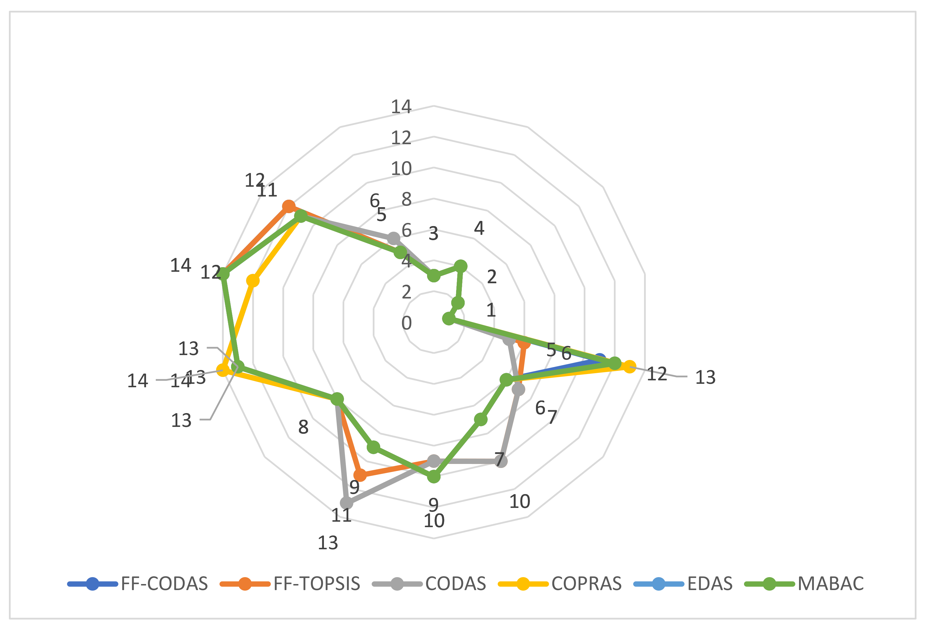
| FF–CODAS | FF–TOPSIS | CODAS | COPRAS | EDAS | MABAC | |
| B1 | 3 | 3 | 3 | 3 | 3 | 3 |
| B2 | 4 | 4 | 4 | 4 | 4 | 4 |
| B3 | 2 | 2 | 2 | 2 | 2 | 2 |
| B4 | 1 | 1 | 1 | 1 | 1 | 1 |
| B5 | 11 | 6 | 5 | 13 | 12 | 12 |
| B6 | 6 | 7 | 7 | 6 | 6 | 6 |
| B7 | 7 | 10 | 10 | 7 | 7 | 7 |
| B8 | 10 | 9 | 9 | 10 | 10 | 10 |
| B9 | 9 | 11 | 13 | 9 | 9 | 9 |
| B10 | 8 | 8 | 8 | 8 | 8 | 8 |
| B11 | 13 | 13 | 14 | 14 | 13 | 13 |
| B12 | 14 | 14 | 12 | 12 | 14 | 14 |
| B13 | 12 | 12 | 11 | 11 | 11 | 11 |
| B14 | 5 | 5 | 6 | 5 | 5 | 5 |
| ρ | 0.912 ** | 0.846 ** | 0.978 ** | 0.996 ** | 0.996 ** | |
| Brand | Hi | After Interchange (FF–CODAS) | Original (FF–CODAS) |
|---|---|---|---|
| B1 | 14.0783 | 3 | 3 |
| B2 | 8.2351 | 4 | 4 |
| B3 | −13.6715 | 12 | 2 |
| B4 | 27.5187 | 1 | 1 |
| B5 | 7.4218 | 11 | 11 |
| B6 | 7.0981 | 6 | 6 |
| B7 | −11.1985 | 7 | 7 |
| B8 | −10.4372 | 10 | 10 |
| B9 | −13.6449 | 9 | 9 |
| B10 | −8.1197 | 8 | 8 |
| B11 | −14.1081 | 13 | 13 |
| B12 | −22.5544 | 14 | 14 |
| B13 | 21.7585 | 2 | 12 |
| B14 | 7.6237 | 5 | 5 |
| Cases (Scheme (i)) | τ Value | ||||||
|---|---|---|---|---|---|---|---|
| Original | 0.02 | ||||||
| Exp 1 | 0.03 | ||||||
| Exp 2 | 0.04 | ||||||
| Exp 3 | 0.05 | ||||||
| Exp 4 | 0.06 | ||||||
| Exp 5 | 0.07 | ||||||
| Exp 6 | 0.08 | ||||||
| Exp 7 | 0.10 | ||||||
| Cases (Scheme (ii)) | Criteria Weights | ||||||
| C1 | C2 | C3 | C4 | C5 | C6 | C7 | |
| Original | 0.1039 | 0.1415 | 0.1649 | 0.1386 | 0.1592 | 0.1416 | 0.1503 |
| Exp 1 | 0.1649 | 0.1415 | 0.1039 | 0.1386 | 0.1592 | 0.1416 | 0.1503 |
| Exp 2 | 0.1039 | 0.1415 | 0.1386 | 0.1649 | 0.1592 | 0.1416 | 0.1503 |
| Exp 3 | 0.1039 | 0.1415 | 0.1592 | 0.1386 | 0.1649 | 0.1416 | 0.1503 |
| Exp 4 | 0.1039 | 0.1386 | 0.1649 | 0.1415 | 0.1592 | 0.1416 | 0.1503 |
| Exp 5 | 0.1039 | 0.1415 | 0.1649 | 0.1386 | 0.1503 | 0.1416 | 0.1592 |
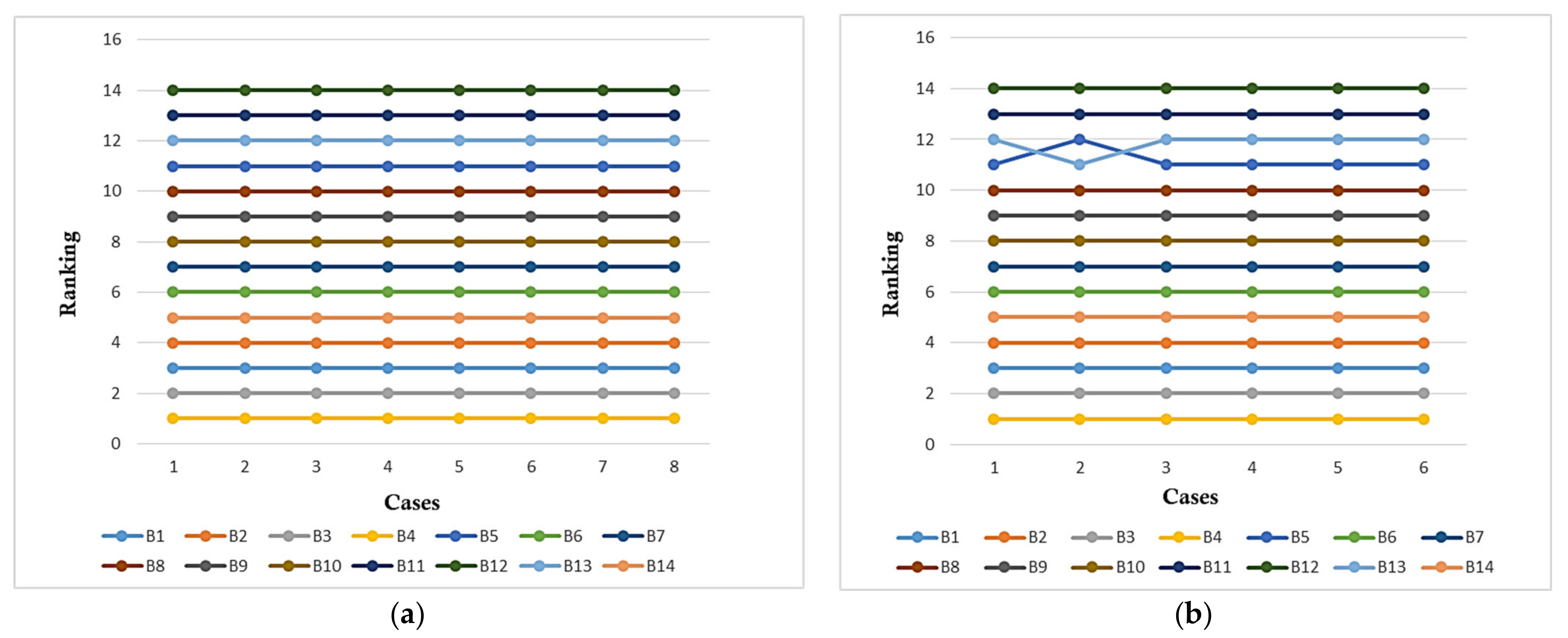
| Brand | Original | Exp 1 | Exp 2 | Exp 3 | Exp 4 | Exp 5 | Exp 6 | Exp 7 |
|---|---|---|---|---|---|---|---|---|
| τ = 0.02 | τ = 0.03 | τ = 0.04 | τ = 0.05 | τ = 0.06 | τ = 0.07 | τ = 0.08 | τ = 0.10 | |
| B1 | 3 | 3 | 3 | 3 | 3 | 3 | 3 | 3 |
| B2 | 4 | 4 | 4 | 4 | 4 | 4 | 4 | 4 |
| B3 | 2 | 2 | 2 | 2 | 2 | 2 | 2 | 2 |
| B4 | 1 | 1 | 1 | 1 | 1 | 1 | 1 | 1 |
| B5 | 11 | 11 | 11 | 11 | 11 | 11 | 11 | 11 |
| B6 | 6 | 6 | 6 | 6 | 6 | 6 | 6 | 6 |
| B7 | 7 | 7 | 7 | 7 | 7 | 7 | 7 | 7 |
| B8 | 10 | 10 | 10 | 10 | 10 | 10 | 10 | 10 |
| B9 | 9 | 9 | 9 | 9 | 9 | 9 | 9 | 9 |
| B10 | 8 | 8 | 8 | 8 | 8 | 8 | 8 | 8 |
| B11 | 13 | 13 | 13 | 13 | 13 | 13 | 13 | 13 |
| B12 | 14 | 14 | 14 | 14 | 14 | 14 | 14 | 14 |
| B13 | 12 | 12 | 12 | 12 | 12 | 12 | 12 | 12 |
| B14 | 5 | 5 | 5 | 5 | 5 | 5 | 5 | 5 |
| Brand | Original | Exp 1 | Exp 2 | Exp 3 | Exp 4 | Exp 5 |
|---|---|---|---|---|---|---|
| B1 | 3 | 3 | 3 | 3 | 3 | 3 |
| B2 | 4 | 4 | 4 | 4 | 4 | 4 |
| B3 | 2 | 2 | 2 | 2 | 2 | 2 |
| B4 | 1 | 1 | 1 | 1 | 1 | 1 |
| B5 | 11 | 12 | 11 | 11 | 11 | 11 |
| B6 | 6 | 6 | 6 | 6 | 6 | 6 |
| B7 | 7 | 7 | 7 | 7 | 7 | 7 |
| B8 | 10 | 10 | 10 | 10 | 10 | 10 |
| B9 | 9 | 9 | 9 | 9 | 9 | 9 |
| B10 | 8 | 8 | 8 | 8 | 8 | 8 |
| B11 | 13 | 13 | 13 | 13 | 13 | 13 |
| B12 | 14 | 14 | 14 | 14 | 14 | 14 |
| B13 | 12 | 11 | 12 | 12 | 12 | 12 |
| B14 | 5 | 5 | 5 | 5 | 5 | 5 |
Publisher’s Note: MDPI stays neutral with regard to jurisdictional claims in published maps and institutional affiliations. |
© 2021 by the authors. Licensee MDPI, Basel, Switzerland. This article is an open access article distributed under the terms and conditions of the Creative Commons Attribution (CC BY) license (https://creativecommons.org/licenses/by/4.0/).
Share and Cite
Biswas, S.; Pamucar, D.; Kar, S.; Sana, S.S. A New Integrated FUCOM–CODAS Framework with Fermatean Fuzzy Information for Multi-Criteria Group Decision-Making. Symmetry 2021, 13, 2430. https://doi.org/10.3390/sym13122430
Biswas S, Pamucar D, Kar S, Sana SS. A New Integrated FUCOM–CODAS Framework with Fermatean Fuzzy Information for Multi-Criteria Group Decision-Making. Symmetry. 2021; 13(12):2430. https://doi.org/10.3390/sym13122430
Chicago/Turabian StyleBiswas, Sanjib, Dragan Pamucar, Samarjit Kar, and Shib Sankar Sana. 2021. "A New Integrated FUCOM–CODAS Framework with Fermatean Fuzzy Information for Multi-Criteria Group Decision-Making" Symmetry 13, no. 12: 2430. https://doi.org/10.3390/sym13122430
APA StyleBiswas, S., Pamucar, D., Kar, S., & Sana, S. S. (2021). A New Integrated FUCOM–CODAS Framework with Fermatean Fuzzy Information for Multi-Criteria Group Decision-Making. Symmetry, 13(12), 2430. https://doi.org/10.3390/sym13122430