New Results of the Time-Space Fractional Derivatives of Kortewege-De Vries Equations via Novel Analytic Method

Abstract

Symmetry performs an essential function in finding the correct techniques for solutions to time space fractional differential equations (TSFDEs). In this article, we present the Novel Analytic Method (NAM) for approximate solutions of the linear and non-linear KdV equation for TSFDs. To enunciate the non-integer derivative for the aforementioned equation, the Caputo operator is manipulated. Furthermore, the formula implemented is a numerical way that is postulated from Taylor’s series, which confirms an analytical answer in the form of a convergent series. For delineation of the efficiency and functionality of the method in question, four applications are exemplified along with graphical interpretation and numerical solutions to finitely illustrate the behavior of the solution to this equation. Moreover, the 3D graphs of some of these numerical examples are plotted with specific values. Observing the effectiveness of this process, we can easily decide that this process can be implemented to other TSFDEs applied in the mathematical modeling of a real-world aspect.

1. Introduction

In recent years, fractional calculus (FC) has drawn a substantial amount of attention in the field of applied mathematics. In financial mathematics, FC is employed in price volatility modeling. Furthermore, Symmetric properties contribute to numerous applications that depend on TSFDEs, such as applications of physics, chemistry, and engineering, so these properties play an important role in knowing the correct way to solve these equations [1,2]. In physics, long particle jumps in anomalous diffusion and the particle motions in a heterogeneous environment were modeled with the help of it. The fast distribution of pollutants in hydrology [3,4], physical phenomena in fluid dynamics [5], biological population and disease models [6], and several other models are well explained within the domain of (ordinary and partial) differential equations of fractional order [7].

In this research paper, we examine the Fractional-Order form of the KdV Equation. The Korteweg-de Vries (KdV) was initially derived by Korteweg and Vries in 1895. It proved to be an exceptional equation and it played a vital role in elaborating several phenomena. The equation in question is regarded as a convenient and frequently used tool to analyze and examine the optical fiber distribution of short laser pulses, meteorological dynamics, and MHD waves. Notably, it exhibits good agreement related to another physical phenomenon, for example, modeling of shallow-water waves, tsunami waves, and acoustic waves, etc. Numerous researchers worked on different aspects of this equation [7,8,9,10]. In [11], the authors discussed higher order KdV with the help of two numerical methods. Numerical solution of KdV Equation by HPM (Homotopy Perturbation Method) and Elazki Transformation has been obtained in [12]. For other details on this equation, see [13,14,15,16,17,18,19].

The present investigation focuses on using the Novel Analytical Method (NAM) as a technique to find the approximate analytical solutions to the Linear and Nonlinear Fractional KdV Equation. This can be considered as an extension and further development of [1,20]. This method involves using Taylor Series as an efficient instrument for solving the nonlinear equations. The proposed method provides Taylor Series solutions by unifying the linear part and nonlinear part together, and then use only calculus of several variables to carry on. This new modification is expected to be more direct and easier to understand, in comparison with the Adomain Decomposition Method. On the other hand, a thorough survey reveals that the Fractional Differential Equation has not been studied as yet using this method. Such are the reasons which provided motivation for the present research to discuss solving the Linear and Non-linear Fractional KdV Equations. This study presents a number of test problems. It also compares the corresponding results with the solutions (already present in literature) to confirm the excellent accuracy of the proposed technique.

The remaining part of this study is as follows: a brief introduction of some important aspects of Fractional Calculus will be given in Section 2. In Section 3, we introduce new Novel Analytic Method (NAM) to construct numerical solutions for the Linear and Non-linear KdV Equation of Fractional Order. Convergence analysis of new Novel Analytic Method (NAM) is discussed in Section 4. Four numerical examples with error tables and graphs are presented in Section 5 to show the efficiency and simplicity of the proposed method. At last, Section 6 concludes the article.

2. Basic Definitions of Fractional Calculus

In this section, we introduce the basic definitions and properties of fractional calculus [21,22,23,24].

Definition 1.

A real function$f\left(x\right),x>0$is said to be in space$C_{\mu } , \mu ϵ \mathcal{R}$if there exists a real number$p>\mu$, such that$f\left(t\right)=t^p f_1\left(t\right)$, where$f_1\left(t\right)\in C\left(0,\infty \right)$, and it is said to be in the space$C_{\mu }^n$if and only if$f^n\in C_{\mu }$, where$n\in N$.

Definition 2.

The Riemann-Liouville fractional integral operator of order$\propto >0$of a function$f\in C_{\mu }$,$\mu >-1,$is defined as

$$j^{\alpha }f\left(t\right)=\frac{1}{\mathsf{\Gamma }\left(\alpha \right)}{{\displaystyle \int }}_o^t{\left(t-s\right)}^{\alpha -1}f\left(s\right)ds ; \alpha >0$$

$$j^{0}f\left(t\right)=f\left(t\right).$$

Recently, many authors have studied different inequalities of Riemann-Liouville fractional integrals; for more details, see [21,22,23,24]. Some properties of the operator$j^{\alpha },$ which are needed here, are as follows:

For$f\in C_{\mu }, \mu \ge -1, \propto ,\beta \ge 0 \mathrm{and} \gamma \ge -1$

$$j^{\propto }{j}^{\beta }f\left(t\right)=j^{\beta +\propto } f\left(t\right)$$

$$j^{\propto }{t}^{\gamma }=\frac{\mathsf{\Gamma }\left(\gamma +1\right)}{\mathsf{\Gamma }\left(\gamma +\alpha +1\right)}{t}^{\alpha +\gamma }$$

Definition 3.

The fractional derivative of f(t) inthe Caputo sense [25] is defined as

$$D^{\alpha }f\left(t\right)=j^{m-\alpha }{D}^{m}f\left(t\right),$$

for .

In Caputo fractional derivative, an ordinary derivative is computed followed by a fractional integral to attain the desired order of fractional derivative.

The Riemann-Liouville fractional integral operator is a linear operation, given as

$$j^{\propto }\left({\displaystyle \sum }_{i-1}^n{c}_i{f}_i\left(t\right)\right)={\displaystyle \sum }_{i=1}^n{c}_{i }{j}^{\propto } f_i\left(t\right),$$

where ${\left\{c_i\right\}}_{i=1}^n$ are constants.

The fractional derivatives are considered in the Caputo sense, in this study.

3. New Novel Analytical Method (NAM) for Fractional Partial Differential Equations (FPDE’S)

In this section, we will introduce the basic ideas of constructing a Novel Analytical Method for the Fractional Partial Differential Equation.

Consider the following general Partial Differential Equation of Fraction Order

$$D_t^{2\alpha }w\left(x,t\right)=\mathcal{F}\left(D_t^{\alpha }w,w,D_x^{\alpha }w,D_x^{2\alpha }w,\cdots \right),$$

(1)

with initial condition

$$w\left(x,0\right)=h_0\left(x\right), D_t^{\alpha }w\left(x,0\right)=h_1\left(x\right).$$

(2)

By using the Fractional Integral for the two sides of Equation (1) from 0 to t, we get

$$D_t^{\alpha }w\left(x,t\right)-D_t^{\alpha }w\left(x,0\right)=I_t^{\alpha } \mathcal{F}\left[w\right]$$

$$D_t^{\alpha }w\left(x,t\right)-h_1\left(x\right)=I_t^{\alpha } \mathcal{F}\left[w\right].$$

Then,

$$D_t^{\alpha }w\left(x,t\right)=h_1\left(x\right)+I_t^{\alpha } \mathcal{F}\left[w\right]$$

(3)

where $\mathcal{F}\left[w\right]=\mathcal{F}\left(D_t^{\alpha }w,w,D_x^{\alpha }w,D_x^{2\alpha }w,\cdots \right).$

Then, when the fractional integral of two sides of Equation (3) is used from 0 to t, we obtain,

$$w\left(x,t\right)-w\left(x,0\right)=h_1\left(x\right)\frac{t^{\alpha }}{\mathsf{\Gamma }\left(\alpha +1\right)}+I_t^{2\alpha } \mathcal{F}\left[w\right]$$

$$w\left(x,t\right)-h_0\left(x\right)=h_1\left(x\right)\frac{t^{\alpha }}{\mathsf{\Gamma }\left(\alpha +1\right)}+I_t^{2\alpha } \mathcal{F}\left[w\right].$$

Thus,

$$w\left(x,t\right)=h_0\left(x\right)+h_1\left(x\right)\frac{t^{\alpha }}{\mathsf{\Gamma }\left(\alpha +1\right)}+I_t^{2\alpha } \mathcal{F}\left[w\right].$$

(4)

The Fractional Taylor series is extended for $\mathcal{F}\left[w\right]$ about t = 0, which is

$$\mathcal{F}\left[w\right]={\displaystyle \sum }_{n=0}^{\infty }\frac{D_t^{n\alpha }\mathcal{F}\left[w_0\right]}{\mathsf{\Gamma }\left(n\alpha +1\right)}{t}^{n\alpha }, \alpha >0$$

$$\mathcal{F}\left[w\right]=\mathcal{F}\left[w_0\right]+\frac{D_t^{\alpha }\mathcal{F}\left[w_0\right]}{\mathsf{\Gamma }\left(\alpha +1\right)}{t}^{\alpha }+\frac{D_t^{2\alpha }\mathcal{F}\left[w_0\right]}{\mathsf{\Gamma }\left(2\alpha +1\right)}{t}^{2\alpha }+\frac{D_t^{3\alpha }\mathcal{F}\left[w_0\right]}{\mathsf{\Gamma }\left(3\alpha +1\right)}{t}^{3\alpha }+\cdots +\frac{D_t^{n\alpha }\mathcal{F}\left[w_0\right]}{\mathsf{\Gamma }\left(n\alpha +1\right)}{t}^{n\alpha }+\cdots$$

(5)

Substituting Equation ($5$) by Equation ($4$), we get

$$w\left(x,t\right)=h_0\left(x\right)+h_1\left(x\right)\frac{t^{\alpha }}{\mathsf{\Gamma }\left(\alpha +1\right)}+I_t^{2\alpha }\left[\mathcal{F}\left[w_0\right]+\frac{D_t^{\alpha }\mathcal{F}\left[w_0\right]}{\mathsf{\Gamma }\left(\alpha +1\right)}{t}^{\alpha }+\frac{D_t^{2\alpha }\mathcal{F}\left[w_0\right]}{\mathsf{\Gamma }\left(2\alpha +1\right)}{t}^{2\alpha }+\frac{D_t^{3\alpha }\mathcal{F}\left[w_0\right]}{\mathsf{\Gamma }\left(3\alpha +1\right)}{t}^{3\alpha }+\cdots +\frac{D_t^{n\alpha }\mathcal{F}\left[w_0\right]}{\mathsf{\Gamma }\left(n\alpha +1\right)}{t}^{n\alpha }+\cdots \right]$$

$$\begin{array}{cc}\hfill w\left(x,t\right)=h_0\left(x\right)& +h_1\left(x\right)\frac{t^{\alpha }}{\mathsf{\Gamma }\left(\alpha +1\right)}+\frac{\mathcal{F}\left[w_0\right]}{\mathsf{\Gamma }\left(2\alpha +1\right)}{t}^{2\alpha }+\frac{D_t^{\alpha }\mathcal{F}\left[w_0\right]}{\mathsf{\Gamma }\left(3\alpha +1\right)}{t}^{3\alpha }+\frac{D_t^{2\alpha }\mathcal{F}\left[w_0\right]}{\mathsf{\Gamma }\left(4\alpha +1\right)}{t}^{4\alpha }+\frac{D_t^{3\alpha }\mathcal{F}\left[w_0\right]}{\mathsf{\Gamma }\left(5\alpha +1\right)}{t}^{5\alpha }+\cdots \hfill \\ & +\frac{D_t^{n\alpha }\mathcal{F}\left[w_0\right]}{\mathsf{\Gamma }\left(\left(n+2\right)\alpha +1\right)}{t}^{\left(n+2\right)\alpha }+\cdots \hfill \end{array}$$

$$w\left(x,t\right)=a_0+a_1\frac{t^{\alpha }}{\mathsf{\Gamma }\left(\alpha +1\right)}+a_2\frac{t^{2\alpha }}{\mathsf{\Gamma }\left(2\alpha +1\right)}+a_3\frac{t^{3\alpha }}{\mathsf{\Gamma }\left(3\alpha +1\right)}+\cdots +a_n\frac{t^{n\alpha }}{\mathsf{\Gamma }\left(n\alpha +1\right)}+\cdots$$

(6)

where,

$$a_0=h_0\left(x\right),$$

$$a_1=h_1\left(x\right),$$

$$a_2=\mathcal{F}\left[w_0\right],$$

$$a_3=D_t^{\alpha }\mathcal{F}\left[w_0\right]$$

$$⋮$$

$$a_n=D_t^{\left(n-2\right)\alpha }\mathcal{F}\left[w_0\right],$$

such that 𝑛 is the highest derivative of $w$. The formal of Equation (6) is to expand Fractional Taylor’s series for 𝑤 about t = 0. This means that,

$$a_0=w\left(x,0\right),$$

$$a_1=D_t^{\alpha }w\left(x,0\right),$$

$$a_2=D_t^{2\alpha }w\left(x,0\right),$$

$$a_3=D_t^{3\alpha }w\left(x,0\right),$$

$$⋮$$

$$a_n=D_t^{n\alpha }w\left(x,0\right).$$

So that we can easily obtained our required numerical solution.

4. Convergence Analysis of Novel Analytical Method (NAM)

Consider PDE as:

$$w\left(x,t\right)=\mathcal{F}\left(w\left(x,t\right)\right)$$

(7)

with $\mathcal{F}$ denoting a nonlinear operator. Then, the following sequence is an equivalent form of the obtained solution:

$$w\left(x,t\right)=\mathcal{F}\left(w\left(x,t\right)\right)$$

(8)

Theorem 1.

Let$\mathcal{G}$be an operator from Hilbert space$ℍ\to ℍ$and$w$be the exact solution of Equation (7). The approximate solution${\displaystyle \sum }_{\mathcal{R}=0}^{𝓅}{w}_{\mathcal{R}}={\displaystyle \sum }_{\mathcal{R}=0}^{𝓅}{\delta }_{\mathcal{R}}\frac{{\left(\Delta t\right)}^{\mathcal{R}}}{\mathcal{R}!}$is converged to exact solution$w$, when $\exists$ a $0\le \delta <1$, $\parallel w_{\mathcal{R}+1}\parallel \le \delta \parallel w_{\mathcal{R}}\parallel \forall \mathcal{R}\in \mathbb{N}\cup \left\{0\right\}$.

Proof. 

We want to prove that ${\left\{{\wp }_{𝓅}\right\}}_{𝓅=0}^{\infty }$ is a converged Cauchy sequence,

$$\parallel {\wp }_{𝓅+1}-{\wp }_{𝓅}\parallel =\parallel w_{𝓅+1}\parallel \le \delta \parallel w_{𝓅}\parallel \le {\delta }^2\parallel w_{𝓅-1}\parallel \le \cdots \le {\delta }^{𝓅}\parallel w_1\parallel \le {\delta }^{𝓅+1}\parallel w_0\parallel$$

(9)

Now for $𝓅,𝓆\in \mathbb{N}, 𝓅\ge 𝓂$ we get

$$\begin{array}{cc}\hfill \parallel {\wp }_{𝓅}-{\wp }_{𝓆}\parallel & =\parallel \left({\wp }_{𝓅}-{\wp }_{𝓅-1}\right)+\left({\wp }_{𝓅-1}-{\wp }_{𝓅-2}\right)+\cdots +\left({\wp }_{𝓆+1}-{\wp }_{𝓆}\right)\parallel \hfill \\ & \le {\wp }_{𝓅}-{\wp }_{𝓅-1}\parallel +\parallel {\wp }_{𝓅-1}-{\wp }_{𝓅-2}\parallel +\cdots +\parallel {\wp }_{𝓆+1}-{\wp }_{𝓆}\parallel \hfill \\ & \le {\delta }^{𝓅}\parallel w_0\parallel +{\delta }^{𝓅-1}\parallel w_0\parallel +\cdots +{\delta }^{𝓆+1}\parallel w_0\parallel \hfill \\ & \le \left({\delta }^{𝓆+1}+{\delta }^{𝓆+2}+\cdots +{\delta }^{𝓅}\right)\parallel w_0\parallel ={\delta }^{𝓆+1}\frac{1-{\delta }^{𝓅-𝓆}}{1-\delta }\parallel w_0\parallel \hfill \end{array}$$

(10)

Hence $\underset{𝓅,𝓆\to \infty }{\lim }\parallel {\wp }_{𝓅}-{\wp }_{𝓆}\parallel =0$, that is, ${\left\{{\wp }_{𝓅}\right\}}_{𝓅=0}^{\infty }$ is a Cauchy sequence in the Hilbert space $ℍ$. Thus, $\exists \mathcal{S}\in ℍ$ s.t $\underset{𝓅\to \infty }{\lim }{\wp }_{𝓅}=\wp$, where $\wp =w$. □

Definition 4.2.

For every$𝓅\in \mathbb{N}\cup \left\{0\right\}$, we define

$${\delta }_{𝓅}=\left\{\begin{array}{cc}\frac{\parallel w_{𝓅+1}\parallel }{\parallel w_{𝓅}\parallel }& \parallel w_{𝓅}\parallel \ne 0\\ 0& otherwise\end{array}\right.$$

(11)

Corollary 4.3. 

From Theorem 1,${\displaystyle \sum }_{\mathcal{R}=0}^{𝓅}{w}_{\mathcal{R}}={\displaystyle \sum }_{\mathcal{R}=0}^{𝓅}{\delta }_{\mathcal{R}}\frac{{\left(\Delta t\right)}^{\mathcal{R}}}{\mathcal{R}!}$is converged to exact solution$w$when$0\le {\delta }_{\mathcal{R}}<1$,$\mathcal{R}=0,1,2,3,\cdots$.

For more detail, see [1,20].

5. Application

In this section, four examples will be solved using the new NAM. The truncated series of the method can be used to calculate the function values numerically. The stability of a method involves analyzing how much the resultant variation occurs in solution when the input parameters of the problem are allowed to vary within certain limits. [26]. We present here the comparison of the NAM with the exact solution at $\alpha =1$ with the help of examples and discuss the stability of the former.

Figure 1 shows two-dimensional plot of the Exact Solution and Approximate Solution using $10th terms$ of NAM in domain $x\in \left[0, 2\pi \right]$ at time $t=0.1$. Figure 2 shows three-dimensional plots of Exact Solution and Approximate Solutions by using proposed technique. Three-dimensional plots of Approximate Solution using NAM between $x$ and $t$ for different values of α are shown in Figure 3. Comparison between Exact Solution and Approximate Solution at different values of $x$ at time $t=0.1, 1.0,2.0, 4.0$ by using NAM is shown in Table 1.

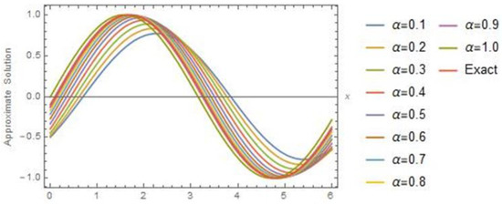
Figure 1. Two-dimensional plots of the Exact solution and Approximate solution using $10th terms$ of NAM versus $x\in \left[0, 2\pi \right]$ at time $t=0.1$ for Example 1.

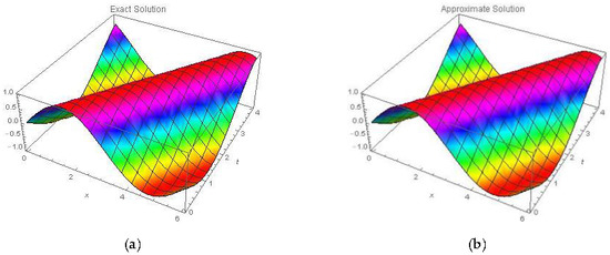
Figure 2. Three-dimensional plots of the (a) Exact solution and (b) Approximate solution using NAM for Example 1.

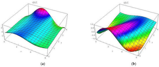
Figure 3. Three-dimensional plots of Approximate Solution using NAM between $x$ and $t$ for (a) α = 0.3 and (b) $\alpha =0.7$ of Example 1.

Table 1. Comparison between Exact solution and Approximate solution at different values of $x$ at $t=0.1,1.0,2.0,4.0$ by using ${10}^{th}\mathrm{term}$ of NAM for Example 1.

$\mathit{t}$	$\mathit{x}$	Exact Solution	Approximate Solution	Absolute Error	$\mathit{t}$	$\mathit{x}$	Exact Solution	Approximate Solution	Absolute Error
0.1	0.00	−0.099833	−0.099833	1.388 × 10−17	1.0	0.00	−0.841471	−0.841471	1.110 × 10−16
	0.25	0.149438	0.149438	0		0.25	−0.681639	−0.681639	1.110 × 10−16
	0.50	0.389418	0.389418	0		0.50	−0.479426	−0.479426	2.220 × 10−16
	0.75	0.605186	0.605186	0		0.75	−0.247404	−0.247404	1.943 × 10−16
	1.00	0.783327	0.783327	0		1.00	0.000000	0.000000	1.665 × 10−16
	1.25	0.912764	0.912764	1.110 × 10−16		1.25	0.247404	0.247404	8.327 × 10−17
	1.50	0.985450	0.985450	1.110 × 10−16		1.50	0.479426	0.479426	5.551 × 10−17
	1.75	0.996865	0.996865	0		1.75	0.681639	0.681639	0
	2.00	0.946300	0.946300	1.110 × 10−16		2.00	0.841471	0.841471	0
	2.25	0.836899	0.836899	0		2.25	0.948985	0.948985	0
	2.50	0.675463	0.675463	1.110 × 10−16		2.50	0.997495	0.997495	1.110 × 10−16
	2.75	0.472031	0.472031	5.551 × 10−17		2.75	0.983986	0.983986	1.110 × 10−16
	3.00	0.239249	0.239249	8.327 × 10−17		3.00	0.909297	0.909297	1.110 × 10−16
	3.25	−0.008407	−0.008407	6.072 × 10−17		3.25	0.778073	0.778073	2.220 × 10−16
	3.50	−0.255541	−0.255541	1.110 × 10−16		3.50	0.598472	0.598472	0
	3.75	−0.486787	−0.486787	5.551 × 10−17		3.75	0.381661	0.381661	2.220 × 10−16
	4.00	−0.687766	−0.687766	1.110 × 10−16		4.00	0.141120	0.141120	1.943 × 10−16
	4.25	−0.845984	−0.845984	2.220 × 10−16		4.25	−0.108195	−0.108195	1.665 × 10−16
	4.50	−0.951602	−0.951602	0		4.50	−0.350783	−0.350783	1.665 × 10−16
	4.75	−0.998054	−0.998054	1.110 × 10−16		4.75	−0.571561	−0.571561	0
	5.00	−0.982453	−0.982453	1.110 × 10−16		5.00	−0.756802	−0.756802	0
	5.25	−0.905767	−0.905767	2.220 × 10−16		5.25	−0.894989	−0.894989	0
	5.50	−0.772764	−0.772764	3.331 × 10−16		5.50	−0.977530	−0.977530	0
	5.75	−0.591716	−0.591716	3.331 × 10−16		5.75	−0.999293	−0.999293	0
	6.00	−0.373877	−0.373877	3.331 × 10−16		6.00	−0.958924	−0.958924	0
2.0	0.00	−0.909297	−0.909297	3.331 × 10−16	4.0	0.00	0.756802	0.756802	2.651 × 10−09
	0.25	−0.983986	−0.983986	6.661 × 10−16		0.25	0.571561	0.571561	1.194 × 10−09
	0.50	−0.997495	−0.997495	1.443 × 10−15		0.50	0.350783	0.350783	4.965 × 10−09
	0.75	−0.948985	−0.948985	2.220 × 10−15		0.75	0.108195	0.108195	8.427 × 10−09
	1.00	−0.841471	−0.841471	2.887 × 10−15		1.00	−0.141120	−0.141120	1.137 × 10−08
	1.25	−0.681639	−0.681639	3.331 × 10−15		1.25	−0.381661	−0.381661	1.360 × 10−08
	1.50	−0.479426	−0.479426	3.664 × 10−15		1.50	−0.598472	−0.598472	1.498 × 10−08
	1.75	−0.247404	−0.247404	3.691 × 10−15		1.75	−0.778073	−0.778073	1.544 × 10−08
	2.00	0.000000	0.000000	3.497 × 10−15		2.00	−0.909297	−0.909297	1.493 × 10−08
	2.25	0.247404	0.247404	3.136 × 10−15		2.25	−0.983986	−0.983986	1.350 × 10−08
	2.50	0.479426	0.479426	2.498 × 10−15		2.50	−0.997495	−0.997495	1.123 × 10−08
	2.75	0.681639	0.681639	1.887 × 10−15		2.75	−0.948985	−0.948985	8.255 × 10−09
	3.00	0.841471	0.841471	7.772 × 10−16		3.00	−0.841471	−0.841471	4.771 × 10−09
	3.25	0.948985	0.948985	0		3.25	−0.681639	−0.681639	9.900 × 10−10
	3.50	0.997495	0.997495	9.992 × 10−16		3.50	−0.479426	−0.479426	2.852 × 10−09
	3.75	0.983986	0.983986	1.776 × 10−15		3.75	−0.247404	−0.247404	6.517 × 10−09
	4.00	0.909297	0.909297	2.665 × 10−15		4.00	0.000000	0.000000	9.777 × 10−09
	4.25	0.778073	0.778073	3.109 × 10−15		4.25	0.247404	0.247404	1.243 × 10−08
	4.50	0.598472	0.598472	3.664 × 10−15		4.50	0.479426	0.479426	1.431 × 10−08
	4.75	0.381661	0.381661	3.719 × 10−15		4.75	0.681639	0.681639	1.530 × 10−08
	5.00	0.141120	0.141120	3.636 × 10−15		5.00	0.841471	0.841471	1.534 × 10−08
	5.25	−0.108195	−0.108195	3.386 × 10−15		5.25	0.948985	0.948985	1.442 × 10−08
	5.50	−0.350783	−0.350783	2.887 × 10−15		5.50	0.997495	0.997495	1.261 × 10−08
	5.75	−0.571561	−0.571561	2.109 × 10−15		5.75	0.983986	0.983986	1.001 × 10−08
	6.00	−0.756802	−0.756802	1.332 × 10−15		6.00	0.909297	0.909297	6.795 × 10−09

Example 1.

Consider the Linearized One-Dimensional Homogeneous Fractional Dispersive KdV Equation,

$$D_t^{\alpha }w\left(x,t\right)+2D_{x}w\left(x,t\right)+D_{xxx}w\left(x,t\right), x\in \left[0,2\pi \right], t\in \left[0,0.1\right]$$

$$w\left(x,0\right)=sinx$$

Following carefully the steps involved in the New Novel-Analytical technique, we arrive at the following series of solutions,

$$\begin{gathered} w\left(x,t\right)=sinx-cosx \frac{t^{\alpha }}{\mathsf{\Gamma }\left(\alpha +1\right)}-sinx\frac{t^{2\alpha }}{\mathsf{\Gamma }\left(2\alpha +1\right)}+cosx\frac{t^{3\alpha }}{\mathsf{\Gamma }\left(3\alpha +1\right)}+sinx\frac{t^{4\alpha }}{\mathsf{\Gamma }\left(4\alpha +1\right)} \\ -cosx\frac{t^{5\alpha }}{\mathsf{\Gamma }\left(5\alpha +1\right)}-sinx\frac{t^{6\alpha }}{\mathsf{\Gamma }\left(6\alpha +1\right)}+\cdots \end{gathered}$$

$$w\left(x,t\right)=sinx{\displaystyle \sum }_{n=0}^{\infty }\frac{{\left(-1\right)}^n t^{2n\alpha }}{\mathsf{\Gamma }\left(2n\alpha +1\right)}-cosx {\displaystyle \sum }_{n=0}^{\infty }\frac{{\left(-1\right)}^n t^{\left(2n+1\right)\alpha }}{\mathsf{\Gamma }\left(\left(2n+1\right)\alpha +1\right)}.$$

The exact solution of this problem is $w\left(x,t\right)=sin\left(x-t\right)$ when $\alpha =1$.

Two-dimensional plots of the Exact Solution and Approximate Solution using $10th terms$ of NAM in domain $x\in \left[0, 6\right]$ at different time $t$ are shown in Figure 4. Three-dimensional plots of Exact Solution and Approximate Solutions by using NAM is shown in Figure 5. By using proposed technique three-dimensional plots of Approximate Solutions between $x$ and $t$ for different values of α are shown in Figure 6. Comparison between Exact Solution and Approximate Solution at different domain values of $x$ at time $t=0.01, 0.05, 0.07,0.10$ by using NAM is shown in Table 2.

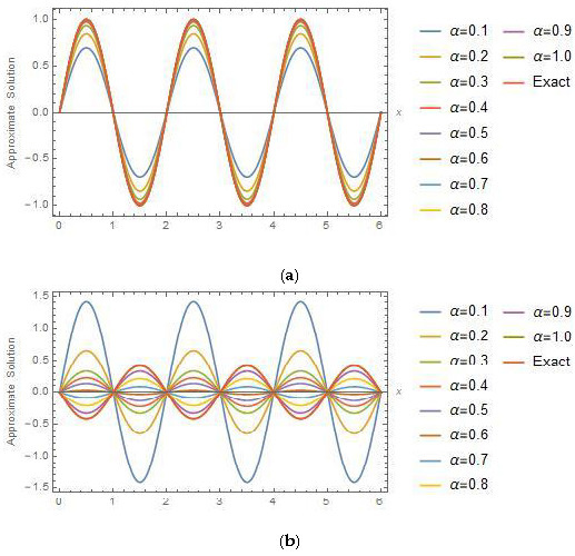
Figure 4. Two-dimensional plots of the Exact Solution and Approximate Solution using $10-terms$ of NAM versus $x\in \left[0, 6\right]$ at time (a) $t=0.01$ and (b) $t=2.0$ for Example 2.

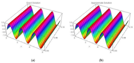
Figure 5. Three-dimensional plots of the (a) Exact Solution and (b) Approximate Solution using NAM for Example 2.

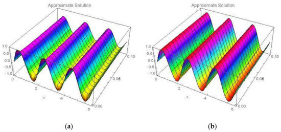
Figure 6. Three-dimensional plots of Approximate Solution using NAM for (a) $\alpha =0.1$ and (b) $\alpha =0.5$ of Example 2.

Table 2. Comparison between Exact Solution and Approximate Solution at different values of $x$ at $t=0.01,0.05,0.07,0.10$ by using $10-\mathrm{terms}$ of NAM for Example 2.

$\mathit{t}$	$\mathit{x}$	Exact Solution	Approximate Solution	Absolute Error	$\mathit{t}$	$\mathit{x}$	Exact Solution	Approximate Solution	Absolute Error
0.01	0.00	0.000000	0.000000	0.000000	0.05	0.00	0.000000	0.000000	0.000000
	0.10	0.309002	0.309002	0.000000		0.10	0.308631	0.308631	0.000000
	0.20	0.587756	0.587756	0.000000		0.20	0.587051	0.587051	0.000000
	0.30	0.808977	0.808977	0.000000		0.30	0.808006	0.808006	0.000000
	0.40	0.951009	0.951009	0.000000		0.40	0.949868	0.949868	0.000000
	0.50	0.999950	0.999950	0.000000		0.50	0.998750	0.998750	0.000000
	0.60	0.951009	0.951009	0.000000		0.60	0.949868	0.949868	0.000000
	0.70	0.808977	0.808977	0.000000		0.70	0.808006	0.808006	0.000000
	0.80	0.587756	0.587756	0.000000		0.80	0.587051	0.587051	0.000000
	0.90	0.309002	0.309002	0.000000		0.90	0.308631	0.308631	0.000000
0.07	0.00	0.000000	0.000000	0.000000	0.10	0.00	0.000000	0.000000	0.000000
	0.10	0.308260	0.308260	0.000000		0.10	0.307473	0.307473	0.000000
	0.20	0.586346	0.586346	0.000000		0.20	0.584849	0.584849	0.000000
	0.30	0.807036	0.807036	0.000000		0.30	0.804975	0.804975	0.000000
	0.40	0.948727	0.948727	0.000000		0.40	0.946305	0.946305	0.000000
	0.50	0.997551	0.997551	0.000000		0.50	0.995004	0.995004	0.000000
	0.60	0.948727	0.948727	0.000000		0.60	0.946305	0.946305	0.000000
	0.70	0.807036	0.807036	0.000000		0.70	0.804975	0.804975	0.000000
	0.80	0.586346	0.586346	0.000000		0.80	0.584849	0.584849	0.000000
	0.90	0.308260	0.308260	0.000000		0.90	0.307473	0.307473	0.000000
	1.00	1.222 × 10−16	1.222 × 10−16	0.000000		1.00	1.219 × 10−16	1.219 × 10−16	0.000000

Example 2.

Consider the Nonhomogeneous Fractional Dispersive KdV Equation of third order,

$$D_t^{\alpha }w\left(x,t\right)+D_{xxx}w\left(x,t\right)=-sin\left(\pi x\right)sint-{\pi }^{3}cos\left(\pi x\right)cost, x\in \left[0,6\right], t>0$$

$$w\left(x,0\right)=sin\left(\pi x\right).$$

With the help of this new technique, we get the following series

$$w\left(x,t\right)=sin\left(\pi x\right)-sin\left(\pi x\right) \frac{t^{2\alpha }}{\mathsf{\Gamma }\left(2\alpha +1\right)}+sin\left(\pi x\right)\frac{t^{4\alpha }}{\mathsf{\Gamma }\left(4\alpha +1\right)}-sin\left(\pi x\right)\frac{t^{6\alpha }}{\mathsf{\Gamma }\left(6\alpha +1\right)}+\cdots$$

$$w\left(x,t\right)=sin\left(\pi x\right) {\displaystyle \sum }_{n=0}^{\infty }\frac{{\left(-1\right)}^n t^{2n\alpha }}{\mathsf{\Gamma }\left(2n\alpha +1\right)}.$$

The exact solution to the above-mentioned problem is $w\left(x,t\right)=sin\left(\pi x\right)cost$ when $\alpha =1$.

The exact solution to this problem is $w\left(x,t\right)=2x+x{t}^3$ when $\alpha =1$. The New NAM is applied, and the exact solution appears in the first few iterations. Two-dimensional and three-dimensional plots of the Exact Solution and Approximate Solution using $10th terms$ of NAM in domain $x\in \left[0, 6\right]$ at different time $t$ are shown in Figure 7 and Figure 8 respectively. By using proposed technique three-dimensional plots of Approximate Solutions between $x$ and $t$ for different values of α are shown in Figure 9. Comparison between Exact Solution and Approximate Solution at different domain values of $x$ at time $t=0.01, 0.05, 0.07,0.10$ by using NAM is shown in Table 3.

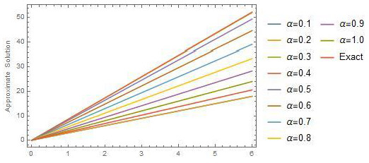
Figure 7. Two-dimensional Plots of the Exact Solution and Approximate Solution using $10-terms$ of NAM versus $x\in \left[0,6\right]$ at time $t=1.0$ for Example 3.

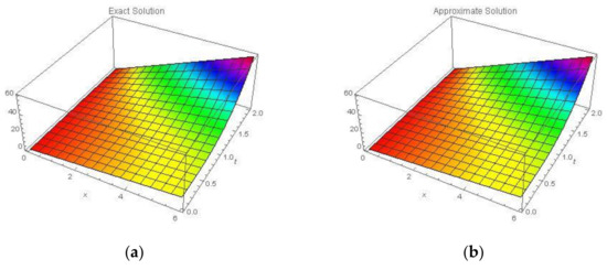
Figure 8. Three-dimensional plots of the (a) Exact Solution and (b) Approximate Solution using NAM for Example 3.

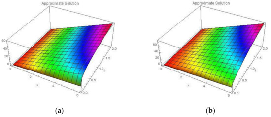
Figure 9. Three-dimensional plots of Approximate Solution using NAM for (a) $\alpha =0.1$ and (b) $\alpha =0.2$ of Example 3.

Table 3. Comparison between Exact Solution and Approximate Solution at some values of $x$ at $t=0.01,0.05,0.07,0.10$ by using $10-\mathrm{terms}$ of NAM for Example 3.

$\mathit{t}$	$\mathit{x}$	Exact Solution	Approximate Solution	Absolute Error	$\mathit{t}$	$\mathit{x}$	Exact Solution	Approximate Solution	Absolute Error
0.01	0.00	0.000000	0.000000	0.000000	0.05	0.00	0.000000	0.000000	0.000000
	0.10	0.200000	0.200000	0.000000		0.10	0.200013	0.200013	0.000000
	0.20	0.400000	0.400000	0.000000		0.20	0.400025	0.400025	0.000000
	0.30	0.600000	0.600000	0.000000		0.30	0.600038	0.600038	0.000000
	0.40	0.800000	0.800000	0.000000		0.40	0.800050	0.800050	0.000000
	0.50	1.000000	1.000000	0.000000		0.50	1.000060	1.000060	0.000000
	0.60	1.200000	1.200000	0.000000		0.60	1.200080	1.200080	0.000000
	0.70	1.400000	1.400000	0.000000		0.70	1.400090	1.400090	0.000000
	0.80	1.600000	1.600000	0.000000		0.80	1.600100	1.600100	0.000000
	0.90	1.800000	1.800000	0.000000		0.90	1.800110	1.800110	0.000000
0.07	0.00	0.000000	0.000000	0.000000	0.10	0.00	0.000000	0.000000	0.000000
	0.10	0.200034	0.200034	0.000000		0.10	0.300000	0.300000	0.000000
	0.20	0.400069	0.400069	0.000000		0.20	0.600000	0.600000	0.000000
	0.30	0.600103	0.600103	0.000000		0.30	0.900000	0.900000	0.000000
	0.40	0.800137	0.800137	0.000000		0.40	1.200000	1.200000	0.000000
	0.50	1.000170	1.000170	0.000000		0.50	1.500000	1.500000	0.000000
	0.60	1.200210	1.200210	0.000000		0.60	1.800000	1.800000	0.000000
	0.70	1.400240	1.400240	0.000000		0.70	2.100000	2.100000	0.000000
	0.80	1.600270	1.600270	0.000000		0.80	2.400000	2.400000	0.000000
	0.90	1.800310	1.800310	0.000000		0.90	2.700000	2.700000	0.000000
	1.00	2.000340	2.000340	0.000000		1.00	3.000000	3.000000	0.000000

Example 3.

Consider the Nonhomogeneous Fractional Dispersive KdV Equation,

$$D_t^{\alpha }w\left(x,t\right)+x D_{x}w\left(x,t\right)+D_{xxx}w\left(x,t\right)=3x{t}^2+2x+x{t}^3, x\in \left[0,1\right], t\in \left[0,1\right]$$

$$w\left(x,0\right)=2x.$$

The numerical solution obtained by Novel Analytical Method is given as

$$w\left(x,t\right)=2x+6x\frac{t^{3\alpha }}{\mathsf{\Gamma }\left(3\alpha +1\right)}.$$

The exact solution of this problem is $w\left(x,t\right)=cos\left(x+y+2t\right)$ when $\alpha =1$. Table 4 shows a comparison between Exact Solution and Approximate Solution at different values of $x$ at $y=0.0, 0.5, 1.0$ and $\mathrm{t}=0.01,0.10$by using NAM. Two-dimensional plots of the Exact Solution and Approximate Solution using $10th terms$ of NAM in domain $x\in \left[0,10\right]$ and $y=0.5$ at times $t=0.01$ and $t=0.1$ are shown in Figure 10. By using proposed technique three-dimensional plots of Approximate Solutions between $x$ and different values of $t$ are shown in Figure 11 and Figure 12 respectively.

Table 4. Comparison between Exact Solution and Approximate Solution at some values of $x$ at $y=0.0, 0.5, 1.0$ and $\mathrm{t}=0.01,0.10$ by using $10-\mathrm{terms}$ of NAM for Example 4.

$\mathit{y}$	$\mathit{t}$	$\mathit{x}$	Exact Solution	Approximate Solution	Absolute Error	$\mathit{t}$	$\mathit{x}$	Exact Solution	Approximate Solution	Absolute Error
0.0	0.01	0.0	0.999800	0.999800	0	0.1	0.0	0.980067	0.980067	0
		1.0	0.523366	0.523366	1.110 × 10−16		1.0	0.362358	0.362358	1.110 × 10−16
		2.0	−0.434248	−0.434248	0		2.0	−0.588501	−0.588501	1.110 × 10−16
		3.0	−0.992617	−0.992617	0		3.0	−0.998295	−0.998295	1.110 × 10−16
		4.0	−0.638378	−0.638378	2.220 × 10−16		4.0	−0.490261	−0.490261	1.665 × 10−16
		5.0	0.302783	0.302783	3.886 × 10−16		5.0	0.468517	0.468517	1.110 × 10−16
		6.0	0.965566	0.965566	0		6.0	0.996542	0.996542	1.110 × 10−16
		7.0	0.740613	0.740613	3.331 × 10−16		7.0	0.608351	0.608351	0
		8.0	−0.165257	−0.165257	4.441 × 10−16		8.0	−0.339155	−0.339155	7.772 × 10−16
		9.0	−0.919190	−0.919190	2.220 × 10−16		9.0	−0.974844	−0.974844	1.110 × 10−16
		10.0	−0.828024	−0.828024	2.220 × 10−16		10.0	−0.714266	−0.714266	5.551 × 10−16
0.5	0.01	0.0	0.867819	0.867819	0	0.1	0.0	0.764842	0.764842	0
		1.0	0.050775	0.050775	1.388 × 10−17		1.0	−0.128844	−0.128844	8.327 × 10−17
		2.0	−0.812952	−0.812952	0		2.0	−0.904072	−0.904072	1.110 × 10−16
		3.0	−0.929254	−0.929254	0		3.0	−0.848100	−0.848100	1.110 × 10−16
		4.0	−0.191204	−0.191204	4.441 × 10−16		4.0	−0.012389	−0.012389	1.596 × 10−16
		5.0	0.722638	0.722638	3.331 × 10−16		5.0	0.834713	0.834713	0
		6.0	0.972090	0.972090	2.220 × 10−16		6.0	0.914383	0.914383	0
		7.0	0.327807	0.327807	4.441 × 10−16		7.0	0.153374	0.153374	1.388 × 10−16
		8.0	−0.617860	−0.617860	3.331 × 10−16		8.0	−0.748647	−0.748647	5.551 × 10−16
		9.0	−0.995470	−0.995470	1.110 × 10−16		9.0	−0.962365	−0.962365	2.220 × 10−16
		10.0	−0.457849	−0.457849	4.441 × 10−16		10.0	−0.291289	−0.291289	6.661 × 10−16
1.0	0.01	0.0	0.523366	0.523366	1.110 × 10−16	0.1	0.0	0.362358	0.362358	1.110 × 10−16
		1.0	−0.434248	−0.434248	0		1.0	−0.588501	−0.588501	1.110 × 10−16
		2.0	−0.992617	−0.992617	0		2.0	−0.998295	−0.998295	1.110 × 10−16
		3.0	−0.638378	−0.638378	2.220 × 10−16		3.0	−0.490261	−0.490261	1.665 × 10−16
		4.0	0.302783	0.302783	3.886 × 10−16		4.0	0.468517	0.468517	1.110 × 10−16
		5.0	0.965566	0.965566	0		5.0	0.996542	0.996542	1.110 × 10−16
		6.0	0.740613	0.740613	3.331 × 10−16		6.0	0.608351	0.608351	0
		7.0	−0.165257	−0.165257	4.441 × 10−16		7.0	−0.339155	−0.339155	7.772 × 10−16
		8.0	−0.919190	−0.919190	2.220 × 10−16		8.0	−0.974844	−0.974844	1.110 × 10−16
		9.0	−0.828024	−0.828024	2.220 × 10−16		9.0	−0.714266	−0.714266	5.551 × 10−16
		10.0	0.024423	0.024423	4.267 × 10−16		10.0	0.203005	0.203005	7.216 × 10−16

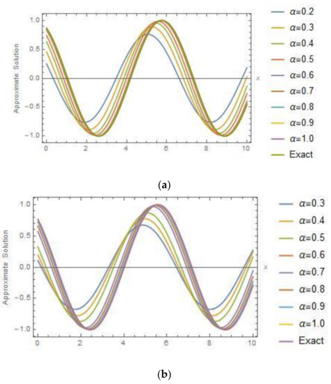
Figure 10. Two-dimensional plots of the Exact Solution and Approximate Solution using $10-terms$ of NAM versus $x\in \left[0,10\right]$ and $y=0.5$ at time (a) $t=0.01$ and (b) $t=0.1$ for Example 4.

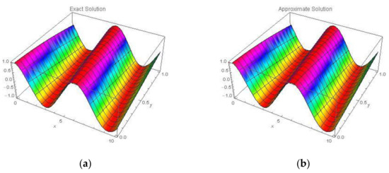
Figure 11. Three-dimensional plots of the (a) Exact Solution and (b) Approximate Solution using NAM for $t=0.1$ of Example 4.

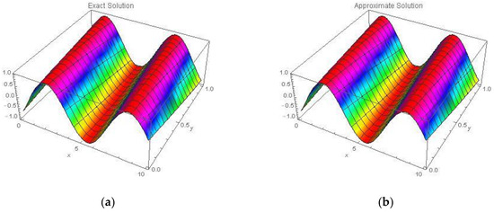
Figure 12. Three-dimensional plots of the (a) Exact Solution and (b) Approximate Solution using NAM for $t=2.0$ of Example 4.

Example 4.

Consider the three-dimensional Fractional Dispersive KdV equation,

$$D_t^{\alpha }w\left(x,y,t\right)+D_{xxx}w\left(x,y,t\right)+D_{yyy}w\left(x,y,t\right)=0, x\in \left[0,10\right], y\in \left[0,1\right],t>0$$

$$w\left(x,y,0\right)=cos\left(x+y\right).$$

Following carefully the steps involved in the new semi-analytical technique, we arrive at the following series of solutions,

$$\begin{gathered} w\left(x,y,t\right)=cos\left(x+y\right)-sin\left(x+y\right)\frac{2t^{\alpha }}{\mathsf{\Gamma }\left(\alpha +1\right)}-cos\left(x+y\right)\frac{4t^{2\alpha }}{\mathsf{\Gamma }\left(2\alpha +1\right)}+sin\left(x+y\right)\frac{8t^{3\alpha }}{\mathsf{\Gamma }\left(3\alpha +1\right)} \\ +cos\left(x+y\right)\frac{16t^{4\alpha }}{\mathsf{\Gamma }\left(4\alpha +1\right)}-sin\left(x+y\right)\frac{32t^{5\alpha }}{\mathsf{\Gamma }\left(5\alpha +1\right)}-cos\left(x+y\right)\frac{64t^{6\alpha }}{\mathsf{\Gamma }\left(6\alpha +1\right)} \end{gathered}$$

To illustrate the results obtained by NAM, we compare these solutions with the ones obtained by the analytical method. The error analysis clearly shows that this method is more convergent and has greater stability compared to its peers Adomain decomposition method and other numerical methods [13,14,15,16,17,18,19].

6. Conclusions

To sum up, we utilized the suggested numerical method NAM to acquire the solution for Fractional-Order KdV Equations. Observing the obtained solutions for the numerical examples, we can conclude that a strong agreement is present with the already prevailing solutions and that this approach can be applied to obtain numerical solutions for the given problems effectively. For computations and simulations, software Mathematica 10 is used. We can also affirm that the errors can be reduced by adding more iterations. The presented numerical solutions have been compared with the exact solution to demonstrate the authenticity and remarkable capability of the introduced numerical method.

References

- Wiwatwanich, A. A Novel Technique for Solving Nonlinear Differential Equations. Ph.D. Thesis, Burapha University, Saen Suk, Chonburi, Thailand, 2016. [Google Scholar]
- Karaçuha, E.; Tabatadze, V.; Karaçuha, K.; Önal, N.Ö.; Ergün, E. Deep Assessment Methodology Using Fractional Calculus on Mathematical Modeling and Prediction of Gross Domestic Product per Capita of Countries. Mathematics 2020, 8, 633. [Google Scholar] [CrossRef]
- Zhang, Y.; Zhou, D.; Wei, W.; Frame, J.M.; Sun, H.; Sun, A.Y.; Chen, X. Hierarchical Fractional Advection-Dispersion Equation (FADE) to Quantify Anomalous Transport in River Corridor over a Broad Spectrum of Scales: Theory and Applications. Mathematics 2021, 9, 790. [Google Scholar] [CrossRef]
- Su, N. Fractional Calculus for Hydrology, Soil Science and Geomechanics; CRC Press: Abingdon, UK, 2020. [Google Scholar]
- Failla, G.; Zingales, M. Advanced materials modelling via fractional calculus: Challenges and perspectives. Phil. Trans. R. Soc. A. 2020, 378, 2172. [Google Scholar] [CrossRef]
- Ionescu, C.M.; Lopes, A.; Copot, D.; Machado, J.A.T.; Bates, J.H.T. The role of fractional calculus in modelling biological phenomena: A review. Commun. Nonlinear Sci. Numer. Simul. 2017, 51, 141–159. [Google Scholar] [CrossRef]
- Panda, S.K.; Ravichandran, C.; Hazarika, B. Results on system of Atangana–Baleanu fractional order Willis aneurysm and nonlinear singularly perturb boundary value problems. Chaos Solitons Fractals 2021, 142, 110390. [Google Scholar] [CrossRef]
- Kaya, D.; Aassila, M. An application for a generalized KdV equation by the decomposition method. Phys. Lett. A 2002, 299, 201–206. [Google Scholar] [CrossRef]
- Saucez, P.; Wouwer, A.V.; Schiesser, W.E. An adaptive method of lines solution of the Korteweg-de Vries equation. Comput. Math. Appl. 1998, 35, 13–25. [Google Scholar] [CrossRef][Green Version]
- Abassy, T.A.; El-Tawil, M.A.; El-Zoheiry, H. Exact solutions of some nonlinear partial differential equations using the variational iteration method linked with Laplace transforms and the Padé technique. Comput. Math. Appl. 2007, 54, 940–954. [Google Scholar] [CrossRef][Green Version]
- Kangalgil, F.; Ayaz, F. Solitary wave solutions for the KdV and mKdV equations by differential transform method. Chaos Solit. Fract. 2009, 41, 464–472. [Google Scholar] [CrossRef]
- Ahmad, H.; Khan, T.A.; Yao, S.W. An efficient approach for the numerical solution of fifth-order KdV equations. Open Math. 2020, 18, 738–748. [Google Scholar] [CrossRef]
- Chavan, S.S.; Panchal, M.M. Solution of third order Korteweg-De Vries equation by homotopy perturbation method using Elzaki transform. Int. J. Res. Appl. Sci. Eng. Technol. 2014, 2, 366–369. [Google Scholar]
- Shah, R.; Khan, H.; Arif, M.; Kumam, P. Application of Laplace Adomian decomposition method for the analytical solution of third-order dispersive fractional partial differential equations. Entropy 2019, 21, 335. [Google Scholar] [CrossRef] [PubMed]
- Othman, M.I.A.; Marin, M. Effect of thermal loading due to laser pulse on thermos-elastic porous medium under GN theory. Results Phys. 2017, 7, 3863–3872. [Google Scholar] [CrossRef]
- Momani, S.; Odibat, Z.; Alawneh, A. Variational iteration method for solving the space and time fractional KdV equation. Numer. Methods Part. Diff. Equat. 2008, 24, 262–271. [Google Scholar] [CrossRef]
- Wang, Q. Homotopy perturbation method for fractional KdV equation. Appl. Math. Comput. 2007, 190, 1795–1802. [Google Scholar] [CrossRef]
- Wang, Q. Homotopy perturbation method for fractional KdV-Burgers equation. Chaos Solit. Fract. 2008, 35, 843–850. [Google Scholar] [CrossRef]
- Momani, S. An explicit and numerical solutions of the fractional KdV equation. Math. Comput. Simulat. 2005, 70, 110–118. [Google Scholar] [CrossRef]
- Ahmad, S.; Ullah, A.; Shah, K.; Akgül, A. Computational analysis of the third order dispersive fractional PDE under exponential-decay and Mittag-Leffler type kernels. Numer. Methods Part. Differ. Eq. 2020. [Google Scholar] [CrossRef]
- Al-Jaberi, A.; Hameed, E.M.; Abdul-Wahab, M.S. A novel analytic method for solving linear and nonlinear Telegraph Equation. Periódico Tchê Química 2020, 17, 536–548. [Google Scholar] [CrossRef]
- Sarikaya, M.Z.; Ogunmez, H. On New Inequalities via Riemann-Liouville Fractional Integration. Hindawi Publ. Corp. Abstr. Appl. Anal. 2012, 2012, 428983. [Google Scholar] [CrossRef]
- Farid, G. Some Riemann–Liouville fractional integral inequalities for convex functions. J. Anal. 2019, 27, 1095–1102. [Google Scholar] [CrossRef]
- Awan, M.U.; Talib, S.; Chu, Y.M.; Noor, M.A.; Noor, K.I. Some New Refinements of Hermite–Hadamard-Type Inequalities Involving ψk-Riemann–Liouville Fractional Integrals and Applications. Hindawi Math. Probl. Eng. 2020, 2020, 3051920. [Google Scholar] [CrossRef]
- Sontakke, B.R.; Shaikh, A.S. Properties of Caputo Operator and Its Applications to Linear Fractional Differential Equations. Int. J. Eng. Res. Appl. 2015, 5, 22–27. [Google Scholar]
- Widatallah, S. A Comparative study on the stability of Laplace-Adomain Algorithm and Numerical methods in generalized Pantograph Equation. Int. Sch. Res. Not. 2012, 2012, 704184. [Google Scholar] [CrossRef]
Publisher’s Note: MDPI stays neutral with regard to jurisdictional claims in published maps and institutional affiliations. |
© 2021 by the authors. Licensee MDPI, Basel, Switzerland. This article is an open access article distributed under the terms and conditions of the Creative Commons Attribution (CC BY) license (https://creativecommons.org/licenses/by/4.0/).