Research on the Detection Method of Tunnel Surface Flatness Based on Point Cloud Data

Abstract

The curved surface of the tunnel is symmetrical. The curved surface of the tunnel can be roughly divided into the left and right arch walls along the direction of the central axis of the tunnel. The symmetry of the tunnel needs to be analyzed when the flatness inspection of the tunnel engineering is carried out. The flatness of the initial support of the tunnel project is an important indicator of the quality inspection and acceptance of the tunnel project. The three-dimensional laser scanner (3DLS) can be used to detect its rapidity effectively. According to the points obtained by the scanner, the surface fitting method based on B-spline interpolation and the SG bar initial support value processing method are used to optimize the tunnel surface to obtain the initial degree calculation reference. Based on the method, a calculation system for the initial flatness of the tunnel based on 3DLS technology is established. At the same time, the calculation method of the overall field of view distance and the development of small blocks is proposed. Through its application and comparison with traditional methods, the analysis shows that the three-dimensional laser scanning technology is feasible in the detection of the initial branch of the tunnel, and achieves a high degree of accuracy requirements.

1. Introduction

The initial support of the tunnel refers to a form of surrounding rock support used on-site to protect the safety of the construction during the excavation of the tunnel project. The flatness refers to the degree of unevenness of the sprayed concrete lining on the initial support surface during the tunnel excavation process [1]. It is one of the important criteria for the quality acceptance of the tunnel project. The results directly affect the subsequent laying of waterproof coiled materials, the paving quality of the second-stage lining, and the safety of the tunnel project; the surface level of the initial support of the tunnel is too large, which directly leads to the decrease of the construction quality of the laying of the waterproof coiled material and the second-stage lining [2]. This indirectly affects the water seepage condition of the tunnel surface, making it more prone to water seepage and leakage in the tunnel. The traditional detection methods for the flatness of the initial tunnels are low in accuracy and efficiency, and fail to meet the expectations of future construction guidance, and the current flatness detection system of the tunnel is not optimistic. The introduction of the emerging 3DLS technology and the establishment of a method system for the flatness detection of the initial support of the tunnel based on the 3DLS technology are of great significance to the improvement and development of the flatness detection system of tunnel engineering [3].

1.1. The Main Work

To establish a detection system for the surface flatness of the initial support of the tunnel based on the 3DLS technology, the tunnel engineering site (Figure 1) was firstly analyzed comprehensively, then a reasonable tunnel engineering measurement plan was formulated. The Topcon GTL-1000 ground 3DLS was used to obtain the data in tunnel engineering. For the surface point cloud data of the initial branch, the relevant parameters of the 3DLS are shown in

Table 1. Performance parameters of the 3D laser scanner.

	Country of Origin	Product Number	Scanning Speed (Point/s)	Range	Ranging Accuracy
3DLS parameters	Japan	GTL-1000	100,000	0.3~1000	2.0 mm@50 m

.

Take the area with a length of 2 m along the central axis of the tunnel as the analysis object, and use the SW Amberg Tunnel to preprocess the collected point cloud data. The SW Amberg Tunnel is specially designed for tunnel construction and was developed by the Swiss Amberg Technology Company (Amberg Technologies) R & D. It supports various tunnel construction methods and construction phase systems. The system is composed of software and hardware. The SW Amberg Tunnel cooperates with and guides high-precision measurement hardware equipment to efficiently and accurately complete the measurement tasks of each construction stage. Not only does it significantly improve the efficiency and accuracy of data collection and analysis, but also achieves an excellent performance in tunneling guidance, high-density scanning section over-under-excavation analysis, refined excavation volume analysis, lining thickness analysis, geotechnical engineering monitoring analysis, and tunnel completion data archiving [4].

After preprocessing by the SW Amberg Tunnel, the point cloud condition of the initial support surface of the tunnel is roughly obtained. It is believed that based on the number of point clouds after the reduction, the random sampling of the point cloud reduction method can maintain the original shape as well as the characteristics of the point cloud. Therefore, a 200 × 200 point cloud data set is obtained by this method and imported into MATLAB. To complete the calculation of the surface flatness of the initial support of the tunnel, the surface fitting method based on B-spline interpolation and the SG filter smoothing method based on curvature correction need to be used to optimize the surface fitting of the point cloud data and obtain the flatness calculation benchmark reference [5]. Finally, the normal vector distance from the original point cloud to the flatness calculation datum is obtained, the calculation formula of the standard deviation and the traditional detection method of the surface flatness of the initial support of the tunnel are presented, and the calculation method of flatness based on 3DLS technology is established. Draw a flatness distribution map based on the calculated flatness. It clarifies the overall and local conditions of the surface flatness of the initial support of the tunnel and improves the entire flatness detection system. It can not only determine the flatness of the surface of the initial support of the tunnel but also determine the uneven surface area of the initial support of the tunnel [6]. The measurement operation of the point cloud data by MATLAB (Commercial mathematics software produced by MathWorks, Natick, MA, USA) is shown in Figure 2.

Through the comparison and analysis with traditional flatness detection methods, the surface flatness detection method of tunnel primary branches based on 3DLS technology not only meets the accuracy requirements and high accuracy, but also meets the requirements of the specification, and its detection method is feasible. The technical route of this research is shown in Figure 3.

1.2. Research Background

The traditional detection methods for the flatness of the initial support of the tunnel mainly include the 2 m leaning ruler combined with the tapered feeler gauge detection method and the total station detection method. Due to the randomness of the selection of detection points, the detection accuracy of this method is not high, the detection speed is slow, and the efficiency is low. When the total station is used to detect the flatness of the initial support surface of the tunnel, the randomness of the selection of detection points and the influence of the prism-free mode on the measurement accuracy will cause the fitted plane to deviate too much from the actual curved surface, which makes it impossible to obtain accurate tunnel flatness. Moreover, the selection of measurement points on the tunnel surface is subjective, so that it cannot comprehensively and truly reflect the condition of the initial support surface of the tunnel [7]. Compared with the traditional methods that have low efficiency, low accuracy, and inconvenient operation, the use of three-dimensional laser scanning technology to detect the surface flatness of the initial support of the tunnel can quickly and accurately obtain the data of the point cloud of the initial support of the tunnel. The operation is simple and does not need to touch the detected surface of the initial support of the tunnel. In addition, the accuracy of the instrument is high enough to meet the specification requirements.

At present, domestic and foreign scholars mainly apply 3D laser technology in the fields of tunnel monitoring and measurement, tunnel overall deformation analysis, etc. The application of 3D laser technology in the flatness detection of tunnel engineering is rarely studied. Duan [8] and others applied 3DLS technology to tunnel monitoring and measurement, and pointed out that when traditional detection methods are used, they are greatly affected by construction, points are easily destroyed, and data is manually recorded and inconvenient for long-term storage. Laser scanning technology has fast measurement speed and no dead ends, which effectively makes up for the shortcomings of traditional monitoring technology. Zhao [9] et al. proposed a dimensionality reduction grid deformation analysis method based on tunnel point cloud data, which can determine the tunnel deformation area and the magnitude of the deformation. Li [10] and others introduced 3DLS technology to collect 3D data of the full section of the tunnel, and qualitatively analyzed the overall deformation through chromatographic analysis, to obtain the deformation of each part of the tunnel more intuitively and automatically. Zhang [11] and others believed that the traditional method of tunnel convergence monitoring has obvious limitations and disadvantages, and clarified that the application of 3DLS technology to tunnel convergence monitoring has better advantages. The comparison with traditional methods shows the feasibility of its method. Weixing [12] and others believe that ground laser scanning technology has a huge development prospect in tunnel engineering, and clarified the advantages of ground laser scanning technology. Jong-SukYoon [13] et al. introduced a method for extracting features of tunnel concrete lining based on 3DLS technology, which provides a theoretical basis for structural health and safety inspection of tunnel construction. Manlin Xiao [14] and others introduced a tunnel surface smoothing algorithm based on mechanics correction, which can be used for 3D point cloud data collected by a 3D laser scanner. Using this algorithm, it is possible to detect and locate the damaged or deteriorated part of the inner wall of the tunnel based on the 3D laser point cloud data, effectively avoiding safety problems. Farahani [15] et al. proposed a three-dimensional laser scanning system, which can effectively obtain the contour of the 3D tunnel model, and set the deformation monitoring of the tunnel through a 3D digital image correlation system suitable for the tunnel structure. Pejić [16] proposed an optimal scheme for effectively measuring the geometry of the tunnel surface through 3DLS technology. This scheme can reliably inspect railway tunnels and achieve the purpose of optimizing the railway tunnel monitoring and measurement system. Fekete [17] and others applied the 3DLS system to the drilling and blasting tunnel operation of railway tunnel projects, which has more advantages than traditional detection methods. At present, there is relatively little research on tunnel flatness detection methods based on 3DLS technology. Therefore, research on tunnel flatness detection methods based on 3DLS technology can provide new technical ideas and methods for tunnel flatness detection.

The calculation method and analysis of the flatness are the keys to how to establish the method for detecting the flatness of the initial support surface of the tunnel based on the three-dimensional laser scanning technology. Many scholars at home and abroad have applied the 3DLS technology to flatness detection. Cheng [18] and others believe that in the engineering survey of the building facade, an electronic total station without cooperation target can be used to fit a plane and calculate the distance from the point to the fitting surface so that the fluctuation of the observation point can be observed. The overall situation can represent the flatness of the building facade. This method is feasible in the measurement of the building facade and meets the accuracy requirements. Li [19] obtained the point cloud data of the building wall according to 3DLS, obtained the accurate wall plane equation and the distance from each point to the fitting plane, and finally calculated and analyzed the wall flatness based on these distances. Based on these values, a distance statistical histogram and a distribution map of the leveling of the wall were made, and the distances were given different colors according to the threshold, which intuitively reflects the leveling of the wall. Li [20] et al. applied the three-dimensional laser scanning technology to the flatness detection of building concrete components, and also developed a color-coded deviation map to indicate the flatness of the components. At the same time, by scanning two different types of concrete components, comparative analysis shows that this method is feasible. Bosché et al. [21] proposed a new method for characterizing the flatness of building surfaces, which relies on the combination of ground laser scanning and continuous wavelet transform. It can provide accurate and extremely dense measurements on the surface of the building, while also providing a method for frequency analysis with high resolution in the spatial and frequency domains. Tang [22] et al. proposed three practical methods for evaluating the flatness of building surfaces through three-dimensional laser scanning technology. Kim [23] et al. proposed a method to detect the surface features and flatness of precast concrete components using building information modeling (BIM) and three-dimensional laser scanning technology. Based on this, a framework for evaluating the surface characteristics and flatness of concrete components is established. Fuchs [24] discussed the feasibility of introducing three-dimensional laser scanning technology into the inspection system of highway bridges, which also includes the inspection of the road smoothness of highway bridges. The research on flatness detection methods based on three-dimensional laser scanning technology is relatively complete. These studies also provide a theoretical basis and ideas for the establishment of the flatness detection system method of the primary surface of tunnel engineering.

1.3. Advantage

The establishment of a tunnel surface flatness detection system based on three-dimensional laser scanning technology is more intuitive and simple to reflect the surface flatness of tunnels. It can provide solid theoretical support and technical guidance for the tunnel engineering construction process thus has very important research significance. It solves the problem that the project in the tunnel does not meet the expectation of future construction guidance and the problem that the existing tunnel engineering initial support flatness detection system is not optimistic. The main innovation of this research is to propose a method for detecting the flatness of the initial support of the tunnel based on the three-dimensional laser scanning technology, introduce the calculation method of the flatness of the initial support of the tunnel, and introduce the concepts of overall flatness and local flatness. The comprehensive analysis of the surface flatness of the initial support of the tunnel through the combination of the overall flatness calculation method and the local flatness calculation method and the flatness distribution diagram has a good guiding role in engineering practice. It also provides research ideas for scholars who study tunnel-related fields [25].

2. Acquisition of Flatness Calculation Datum

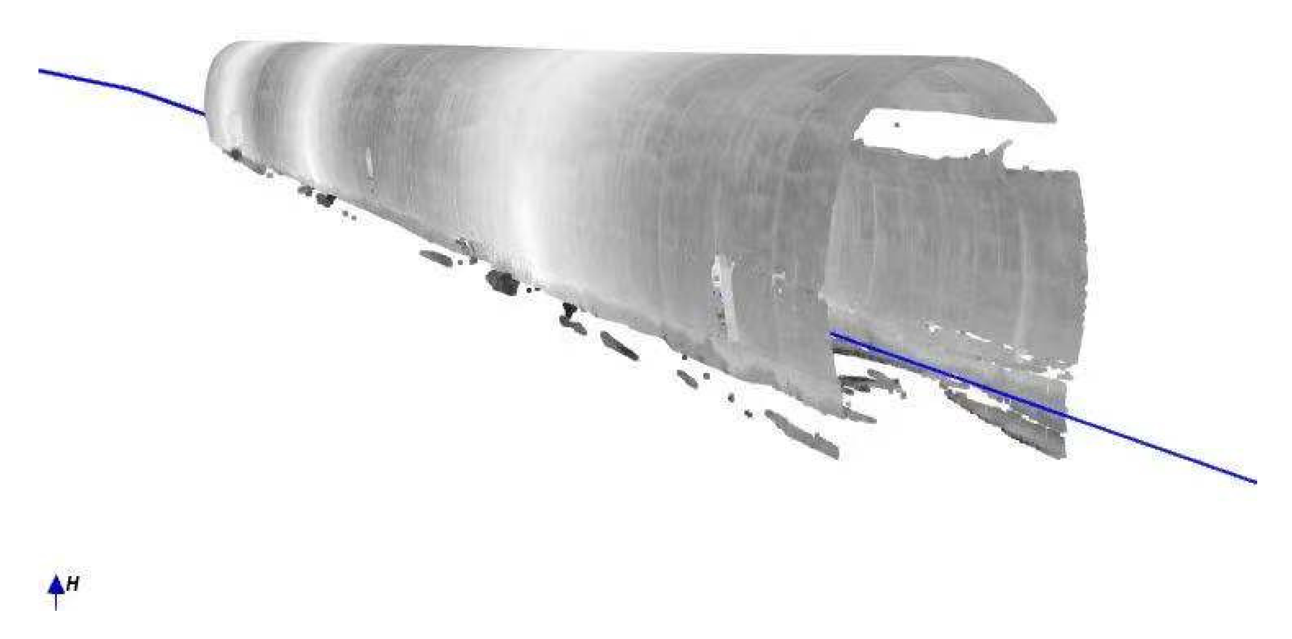
To establish a detection system for the surface flatness of the initial support of the tunnel based on the three-dimensional laser scanning technology, the acquisition of the flatness calculation datum is very important. The point cloud of the tunnel after preprocessing (Figure 4) is very smooth, which is conducive to the reconstruction of the tunnel model. The reconstruction of the tunnel point cloud model is essentially the surface fitting of the point cloud, and the discrete point cloud is fitted to a curved surface that approximates the surface of the target object. The accuracy of the fitted surface also directly affects the calculation of the flatness of the initial support surface of the tunnel result. The flatness calculation datum surface is essentially a fitting surface suitable for flatness calculation obtained by the point cloud data through the fitting method and optimization processing. To obtain the flatness calculation reference surface, selecting a suitable fitting method can effectively improve the degree of fitting optimization.

2.1. Comparison of Fitting Methods

Common surface fitting methods include the meshing method [26], Poisson surface reconstruction method [27], Lagrangian interpolation method [28], and cubic spline interpolation method [29]. This experiment uses 3DLS The instrument obtains the surface point cloud data of the initial branch of the tunnel K109+870~K109+900 in the tunnel project, and takes the point cloud data of some areas as the analysis object, and compares and analyzes the fitting degree and fitting of the four methods when constructing the surface. Accuracy. In the schematic diagram of the degree of surface fitting by the four fitting methods, the X axis represents the direction along the central axis of the tunnel, the Y axis represents the horizontal direction of the tunnel cross-section, and the Z axis represents the vertical direction of the tunnel cross-section. In the schematic diagram, only the intercept Part of the area on the surface of the tunnel.

(1) The degree of fit of the four methods

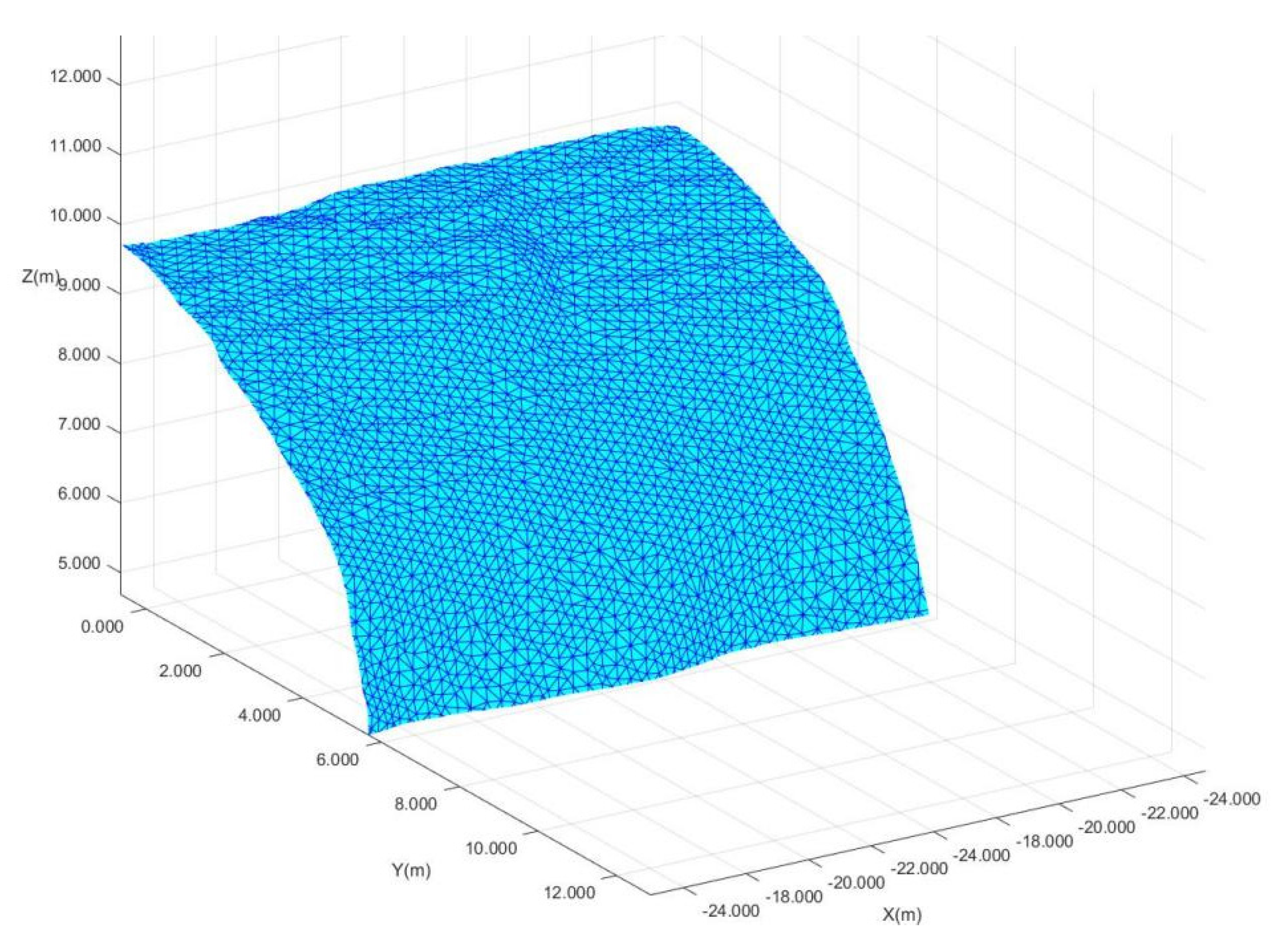
After the tunnel surface is constructed by meshing (Figure 5), the surface is complete and has good continuity, but the smoothness of the surface is poor, and the details of the local area are not enough.

The tunnel surface obtained by the Poisson reconstruction method (Figure 6) is continuous and complete, which can reflect the unevenness of the tunnel surface, but the smoothness of the surface is not high, and the construction details of the point cloud cavity are insufficient.

The tunnel surface constructed by the Lagrangian interpolation method (Figure 7) can reflect the overall contour of the tunnel surface and can reflect the basic details of the tunnel surface in a local area. However, the smoothness of the surface constructed by this method is poor, and there are convex hulls. Phenomenon.

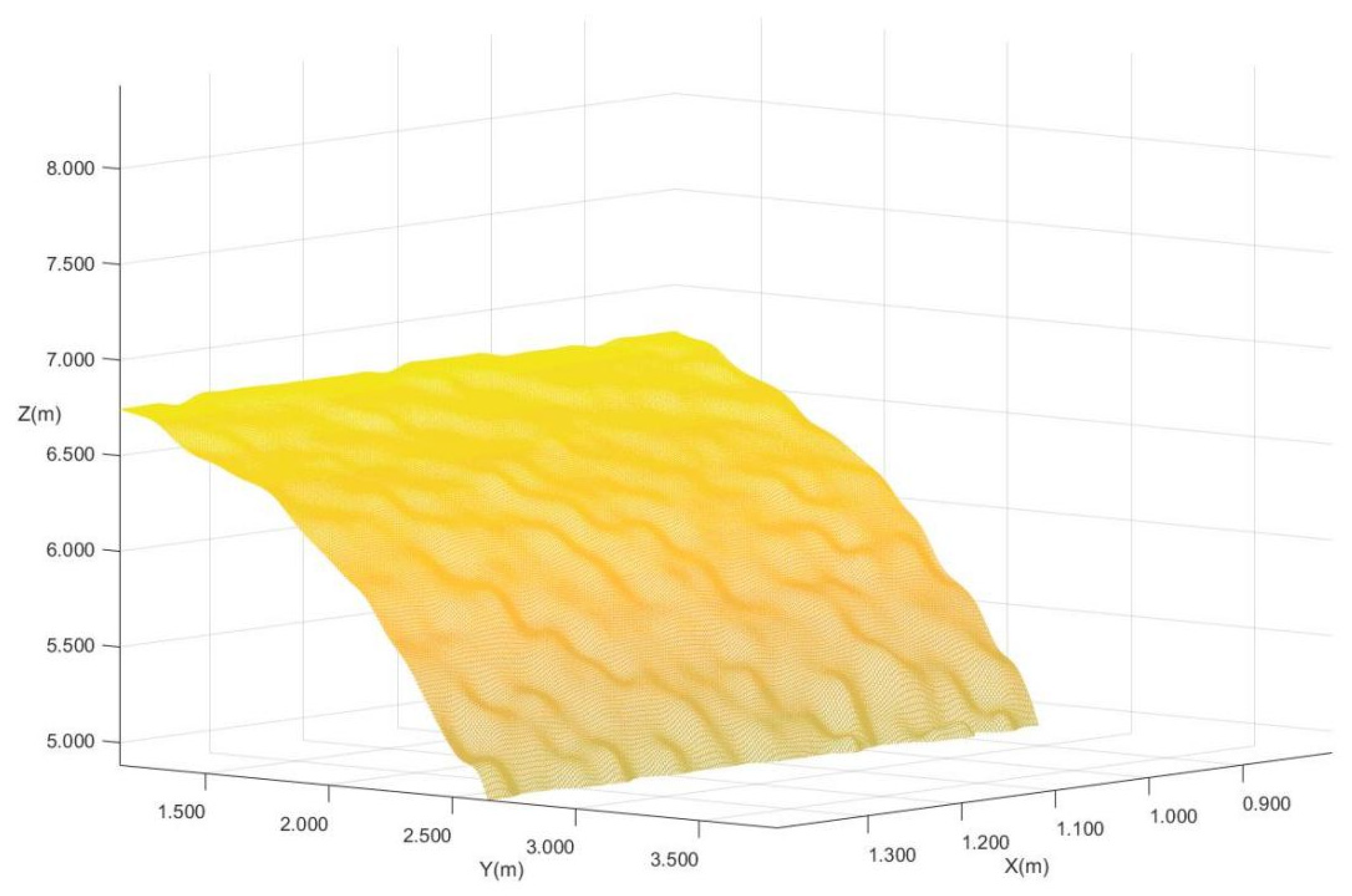
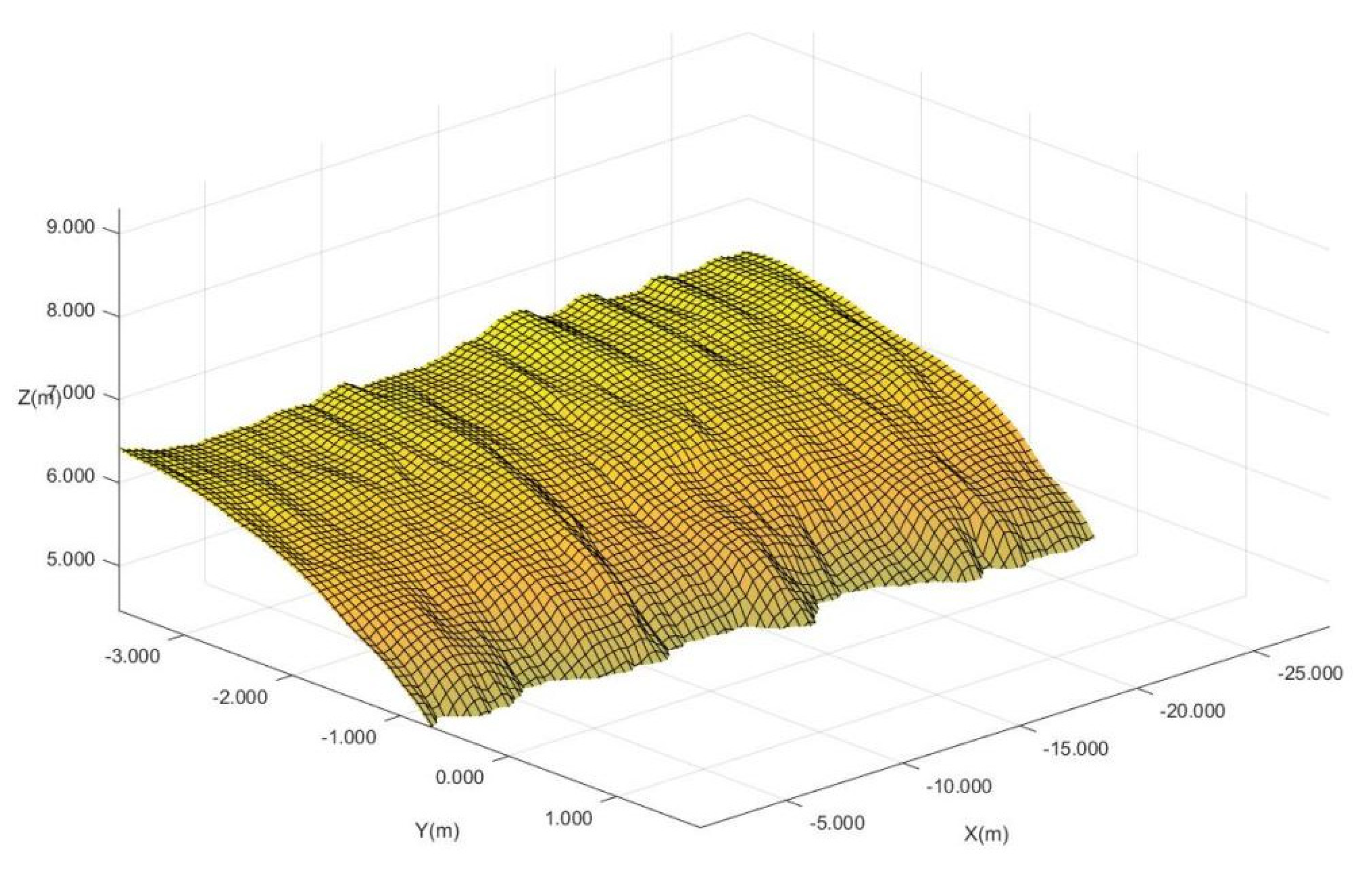
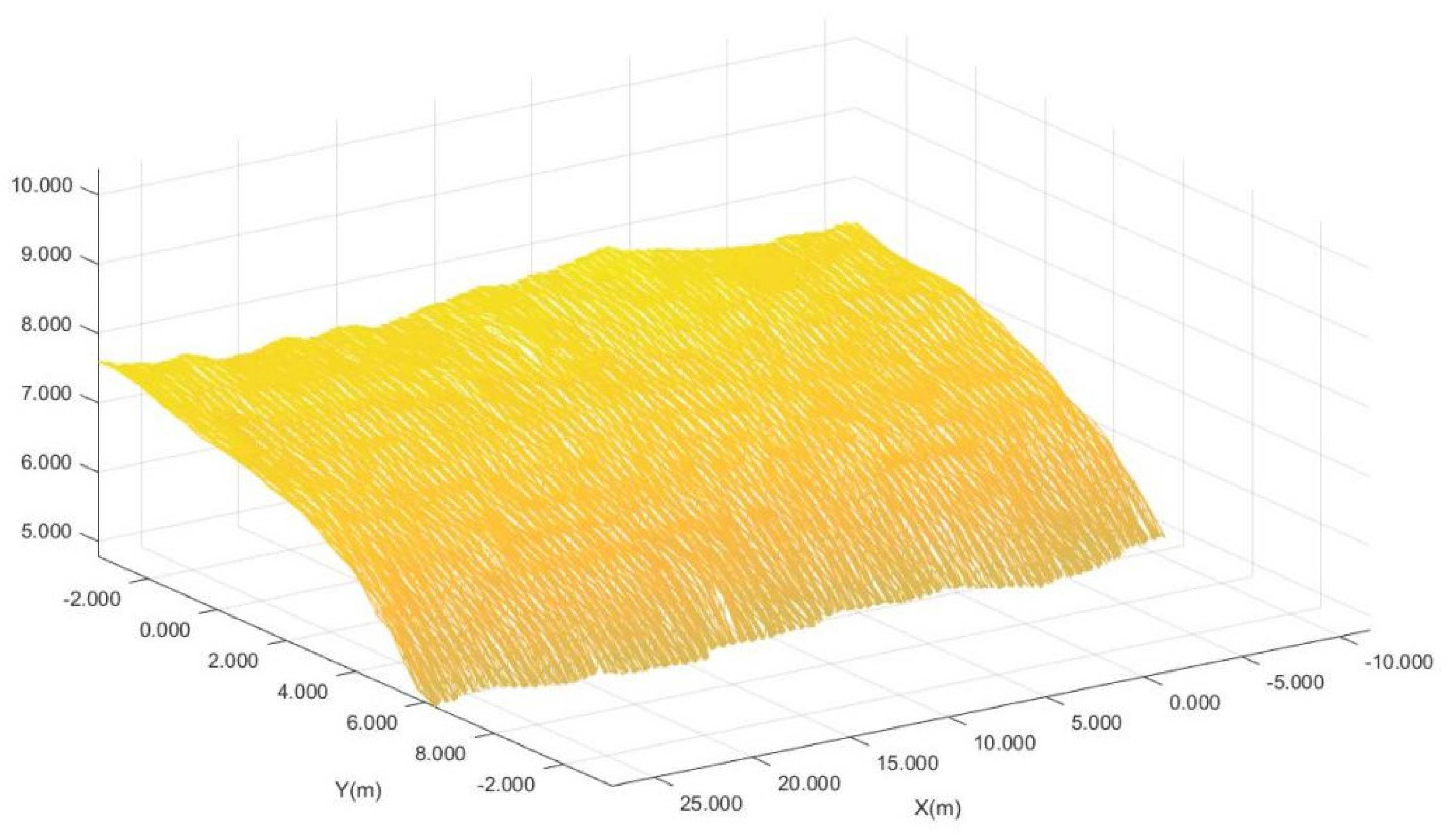
The tunnel surface constructed by the cubic B-spline interpolation method (Figure 8) is continuous and complete, with high smoothness, no local mutations, etc., and the details of the local area are rich, and the tunnel surface is better restored.

(2) Analysis of the fitting accuracy of the four methods

The data this time is a total of 40,000 point clouds. The data points are extracted 5 times from the point cloud data at 5 cm intervals and 100 data points are randomly selected each time, which is divided into 5 groups. After that, the z value corresponding to each point is stored in the order of arrangement, and then the surface is constructed using four methods for the 10 cm interval point cloud data. The x and y of each stored point on the surface correspond to the corresponding z value, 5 cm interval points are compressed to get 10 cm interval point clouds, so the z value on the surface obtained by the 10 cm interval point cloud fitting is different from the corresponding z values of the points stored in the 5 cm interval point cloud. According to the x and y of the stored point, the corresponding surface can be obtained and stored, and then the difference of the corresponding point is calculated. This method is equivalent to the error calculation of the 10 cm interval point cloud, by calculating the sum of each point The fitting difference value corresponding to the fitting surface, the fitting difference value formula is

$$E=z_p-z_p^{\prime }$$

(1)

where: p = 1, 2, 3, …, n.

The fitting error generated by the constructed surface can also be called the root mean square error. By counting the root mean square error, you can get the error of the area where the surface other than the original point is located. The root mean square error formula is:

$$\sigma =\sqrt{\frac{E_1^2+E_2^2+\dots \dots +E_N^2}{n}}=\sqrt{\frac{{\displaystyle \sum E_p^2}}{n}}$$

(2)

According to Formula (2), four interpolation methods are used to construct the surface, and the fitting error is calculated based on 5 sets of data, as shown in

Table 2. Fitting errors of the four sets of data corresponding to the four methods.

$\mathbf{Fitting}\mathbf{Error}\mathit{\sigma }$	Method 1 (mm)	Method 2 (mm)	Method 3 (mm)	Method 4 (mm)
Group 1	3.024	0.995	1.814	1.009
Group 2	3.071	1.015	1.775	0.984
Group 3	3.043	1.044	1.823	1.020
Group 4	3.068	1.007	1.814	1.005
Group 5	3.108	0.980	1.814	0.990

Note: Method 1 means meshing method, method 2 means Poisson reconstruction method, method 3 means Lagrangian interpolation method, method 4 means bicubic spline interpolation method.

.

It can be seen from the tab that the point cloud fitting errors of the Poisson reconstruction method and cubic B-spline interpolation method are kept in a small range, and the fitting accuracy is high. The fitting accuracy of the Lagrangian interpolation method is not high. The grid division method has the largest fitting error and the lowest precision. The results show that the construction of tunnel surface by the Poisson reconstruction method and cubic B-spline interpolation method has higher fitting accuracy.

By comparing and analyzing the fitting degree and fitting accuracy of the four fitting methods when constructing the surface, the following conclusions are drawn: the smoothness of the surface constructed by the meshing method is poor, and the fitting accuracy is low; Poisson reconstruction The fitting accuracy of the method is high, but the surface lacks a certain degree of smoothness; the surface fitting effect constructed by the Lagrangian interpolation method is better, but the fitting accuracy is not high; the cubic B-spline interpolation method has high fitting accuracy, compared with other methods, the surface details are complete and the smoothness is higher. This method has more advantages in the construction of the tunnel surface and has the least influence on the calculation results of the surface flatness of the initial support of the tunnel.

2.2. Optimal Fitting of Cubic B-Spline Interpolation

The main ideas for the optimal fitting of the original point cloud of the tunnel based on the cubic B-spline interpolation method are:

The point cloud data is divided into slices according to the x-direction, that is, the tunnel axis direction, which is equivalent to taking a tiny dx as the threshold. The x coordinate changes of the point cloud data within this range are considered to be on a 2-dimensional slice point. Then perform spline curve-fitting on this two-dimensional slice. First, convert Cartesian coordinates to polar coordinates. Since the cross-section of the tunnel is a curve similar to an arc, after changing to polar coordinates, it can be ensured that the depression angle and the polar radius can be in a one-to-one correspondence. Then use polar coordinates for interpolation and encryption based on the spline curve, and then convert the polar coordinates back to rectangular coordinates to complete the fitting of each section of the tunnel. For the same reason, perform the above processing again in the Y direction. After processing, the curve interpolation is carried out in the two orthogonal directions of the tunnel x and y, and the interpolation in the two directions is superimposed to form the fitting surface of the first branch surface of the tunnel [30].

The method of two-way slice complementary to the overall surface of the tunnel proposed in this study effectively eliminates the jagged layering effect of the one-way slice on the overall fitting surface of the tunnel, and the enlarged tunnel surface appears smoother. The cloud fitting operation speed is also faster than the overall point cloud fitting surface [31].

2.3. S-G Filter Smoothing Based on Curvature

The curved surface after the fitting process by cubic B-spline interpolation has a high degree of smoothness, good continuity, and more complete and rich local details, which is more consistent with the actual engineering situation. However, the fitted surface still has many point clouds that deviate from the actual surface, and its accuracy cannot meet the requirements of flatness calculation. To make the final fitting surface that can meet the requirements of flatness calculation, the fitting surface should not only be close to the actual situation but also ensure that the fitting surface has sufficient smoothness. To further limit the smoothness and authenticity of the fitted surface, this study guarantees the reliability of the fitted surface by limiting the curvature of each point on the fitted surface. Based on the fitting processing of cubic B-spline interpolation, The fitted surface is again processed by SG filtering based on curvature limitation [32]. In all tunnel projects, the design parameters of the Leicaoshan Tunnel are universal, and among many tunnels, Leicaoshan Tunnel is the most typical. The flatness detection method in this study specifies the upper and lower limits of the tunnel point cloud curvature as the curvature parameter value of the Leicaoshan Tunnel. That is, the upper limit is specified as the maximum curvature of the vault in the design parameters of Leicaoshan Tunnel, 0.395, and the lower limit is specified as the minimum curvature of the arch bottom in the design parameters of Leicaoshan Tunnel, 0.104.

The specific plan for curvature limitation is as follows:

(1) First, the curvature of any point on the curve is calculated by the curve function. The curvature of a point is calculated based on the first and second derivatives of the two points before and after. Since the fitted surface obtained by the B-spline interpolation method is fitted by the slicing method, the curvature in this step is also used in the same way. The two-dimensional curvature of each tangent surface in the previous B-spline interpolation method is calculated. Superimposed to form the curvature of the entire surface, the formula for calculating the curvature is as follows:

$$K=\frac{\left|y^{"}\right|}{{\left(1+y^{\prime 2}\right)}^{3/2}}$$

(3)

In the formula, K is the curvature at a point on the curve, and y is the function of the corresponding curve.

(2) There are points in the calculated surface point cloud curvature that are not within the limited range. At this time, it is necessary to perform smoothing and filtering again on the surface obtained by the B-spline interpolation method. For the cross-sectional direction and the longitudinal direction, the data in the two directions is smoothed and filtered again. Taking into account the symmetry of the tunnel and the requirements for the calculation of the surface flatness of the initial support of the tunnel, Savitzky–Golay filtering is used here. The processing of S-G filtering maintains the best shape of the original data, making the processed surface closer to the actual engineering situation.

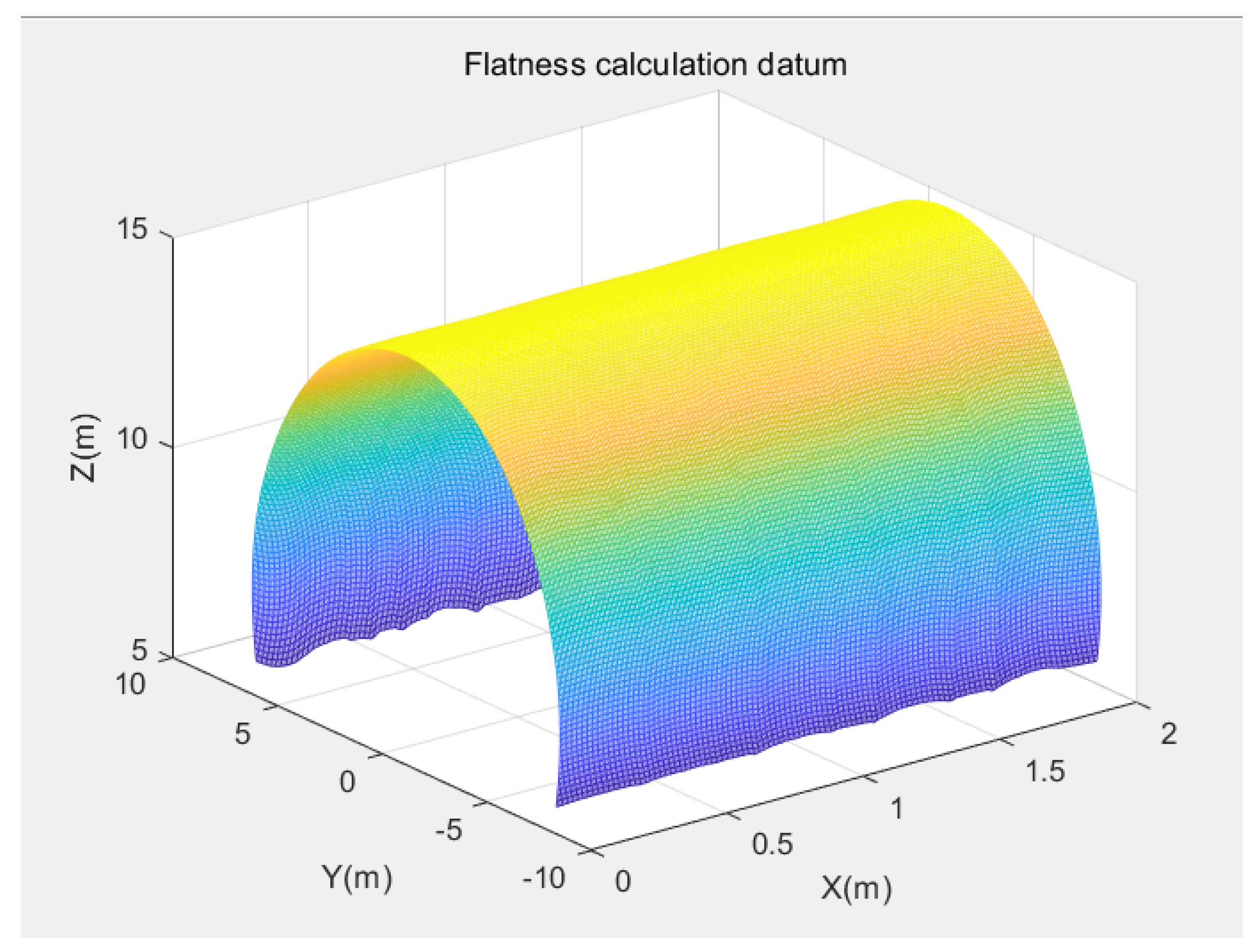
(3) After removing the unqualified points through the above method, the remaining unqualified points are only the points at the bottom of the arch. Because the curvature calculation is calculated using the curvature of the front and back slices, the curvature calculated at the two ends of the point cloud data, namely the two arch bottoms on the left and right, is meaningless in itself, and it can be directly eliminated. At this point, the final flatness calculation datum (Figure 9) is obtained surface. In the figure, the X axis direction represents the direction along the central axis of the tunnel, the Y axis represents the horizontal direction of the tunnel cross-section, and the Z axis represents the vertical direction of the tunnel cross-section. Segment fitting surface.

3. Flatness Calculation

Through the above method, the flatness calculation reference surface has been obtained. The flatness calculation method in this article is based on the normal vector distance from the original point cloud of the initial support surface of the tunnel to the flatness calculation datum plane. The calculation of the normal vector distance only needs to use the original point cloud to make a normal ray perpendicular to the flatness calculation datum plane. The normal ray and the fitted surface intersect at a point, and the distance between this point and the starting point of the ray is the normal vector distance di. Flatness calculation can be divided into two parts: overall flatness and local flatness. The calculation of overall flatness is to analyze the unevenness of the overall point cloud in a region, and the calculation of local flatness is to analyze the point cloud on the local details of a region. The degree of unevenness.

3.1. Overall Flatness

The overall flatness of the initial support surface of the tunnel is mainly determined by the dispersion degree of the normal vector distance from the original point cloud to the flatness calculation datum. If the dispersion is large, it means that the original point cloud and the flatness calculation datum are quite different. The rougher the surface. If the degree of dispersion is small, it means that the difference between the original point cloud and the flatness calculation reference plane is small, and the surface is flatter.

To intuitively express the overall flatness of the surface of the initial support of the tunnel, the concept of standard deviation is introduced. Simply put, the standard deviation is a measure of the degree to which a set of values are scattered from the average. A larger standard deviation means that the difference between most of the values and its average is larger; a smaller standard deviation means that these values are closer to the mean.

To sum up, the formula for calculating the overall flatness of the initial support surface of the tunnel is as follows:

$$m_0=\pm \sqrt{\frac{{\displaystyle \sum d_i^2}}{n-1}}\left(i=1,2,\cdots ,n\right)$$

(4)

In the formula, m₀ is the overall flatness of the initial support surface of the tunnel, di is the normal vector distance, and n is the no. of point clouds collected during flatness detection.

3.2. Local Flatness

The overall flatness of the surface of the initial support of the tunnel can only reflect the overall flatness of a specific section of the tunnel. In a specific tunnel project, the overall flatness of the surface of the first support of the tunnel can only play a qualitative role, but cannot pass a quantitative one. Method to define the leveling degree of the specific local location of the tunnel surface. Therefore, the concept of local flatness is introduced, and the uneven points on the local details of the initial support surface of the tunnel are expressed through the concept of local flatness.

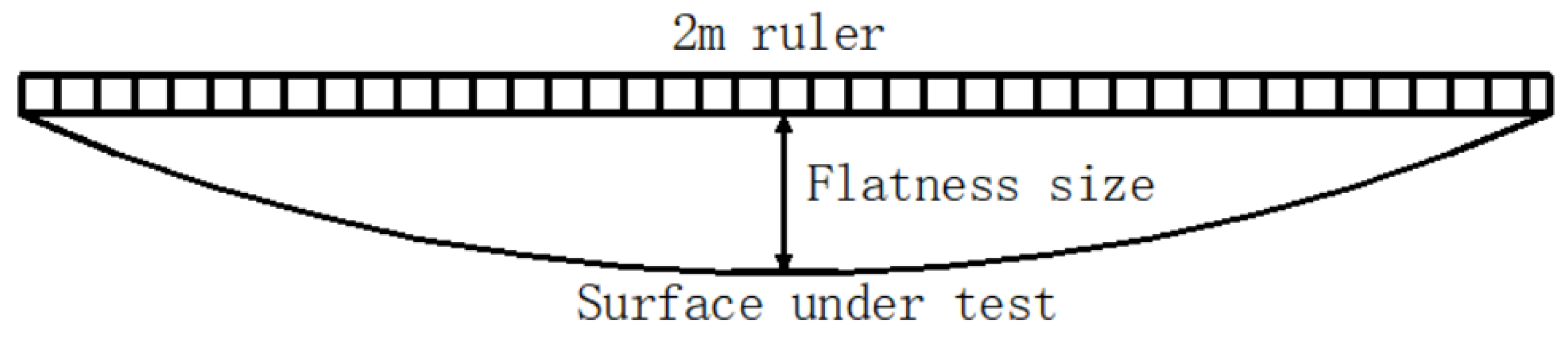
In the traditional method of detecting the surface flatness of the initial support of the tunnel, the 2 m ruler method is generally used to define the flatness: the maximum gap value between the reference plane of the 2 m ruler and the measuring surface. Usually, two points are measured every 200 m, and each point is continuously tested 10 times. According to the qualified rate, it is judged whether the surface flatness meets the measurement requirements. The schematic diagram for defining the flatness of the 2 m leaning rule method is shown in Figure 10.

By referring to the flatness definition method in the 2 m ruler method, this paper introduces the local flatness definition method based on 3DLS technology:

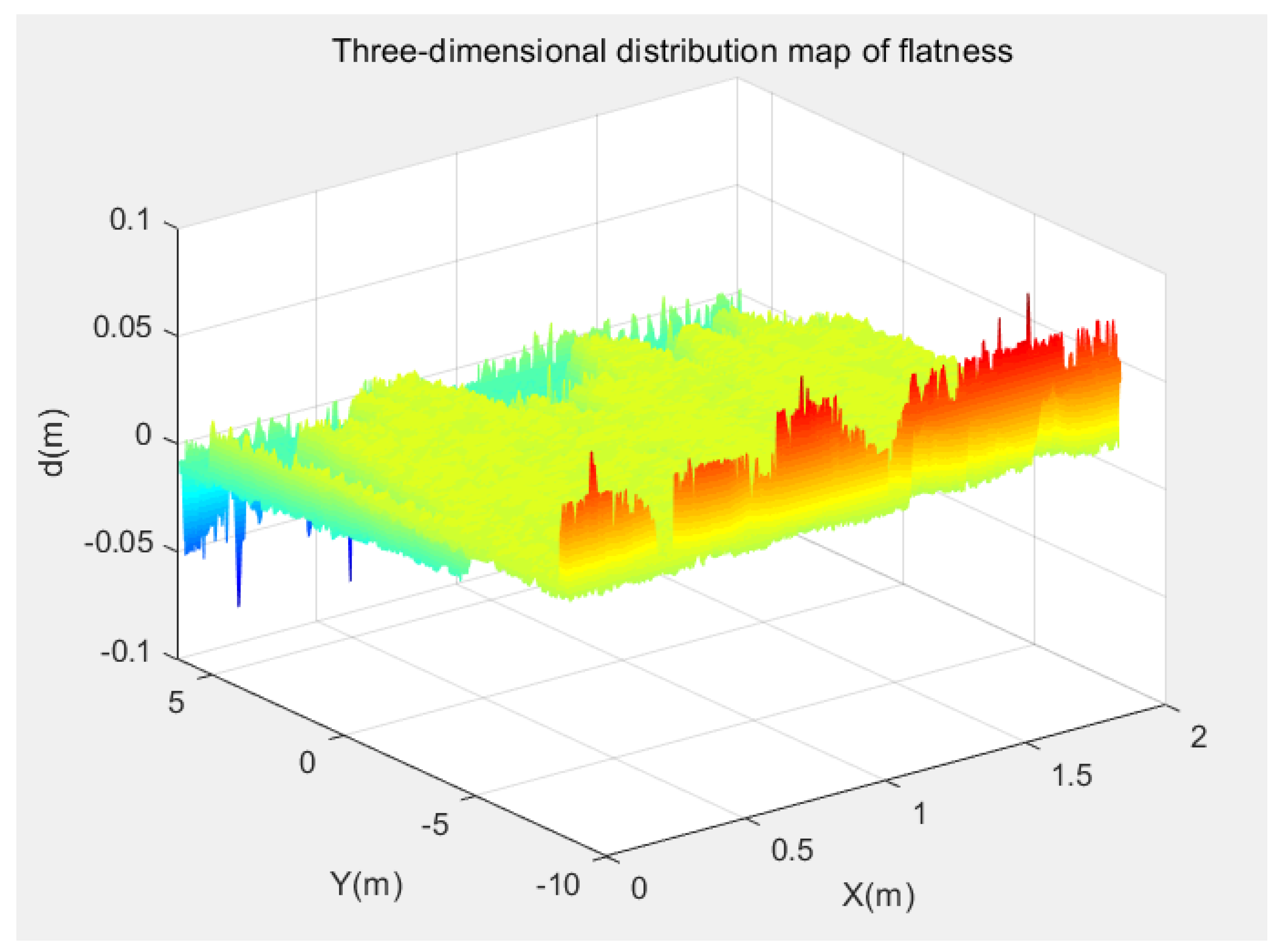
(1) First obtain the three-dimensional distribution map of flatness as shown in Figure 11, where the X axis represents the direction of the tunnel’s central axis, the Y axis represents the direction of the tunnel cross-section, and the Z axis represents the normal vector distance of the original point cloud and flatness calculation reference plane. Flatness situation. It can be clearly seen from the three-dimensional map of flatness that the flatness of the tunnel has symmetry along the direction of the tunnel’s central axis (Y = 0). The flatness of the left arch of the tunnel is mostly on the negative Z semi-axis, and the flatness of the right arch of the tunnel is mostly on the positive Z semi-axis.

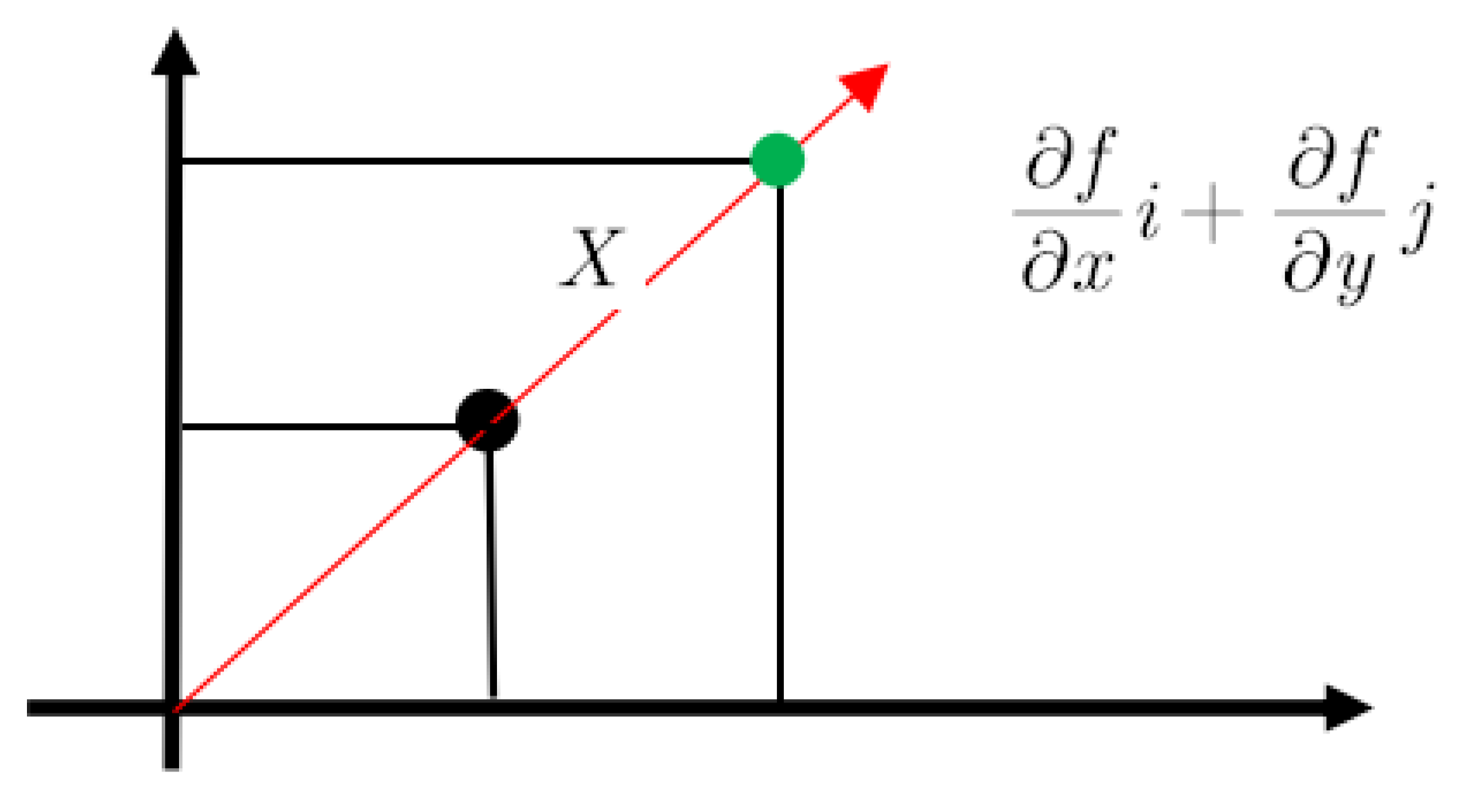
(2) The flatness data in the Figure constitutes a 3-dimensional scalar field. First, calculate the gradient value of this scalar data point at each point. However, the size of this gradient is of no practical significance to the calculation of local flatness here, because what needs to be known here is only the direction of the gradient. Theoretically, every point on a three-dimensional surface has countless directions that can be changed, and the gradient of each point is calculated only to obtain the direction with the largest change in flatness.

(3) As it is the gradient of a 2-variable function, the value obtained corresponds to the components in the x-direction and the y-direction, which is as follows:

$$grad\left(f\right)=\frac{\partial f}{\partial x}i+\frac{\partial f}{\partial y}j$$

(5)

In this way, the direction of the gradient vector can be determined based on the x component and the y component, and the direction angle of the gradient can also be obtained.

(4) The flatness distribution map drawn according to the normal vector distance is similar to the topographic map. Here we draw on the principle of slope in the topographic map, slope = elevation difference/horizontal distance, in the gradient direction of each point, calculate the slope i and the inclination angle. The distance X can be adjusted according to the accuracy requirements.

(5) Once the horizontal distance is determined, the height difference between the two points can be known. It can be imagined that a certain point is the center of the circle, the horizontal distance is the radius, and the gradient direction is unique. In the gradient direction, the height changes the fastest, and the highest height difference is obtained when the horizontal distance is constant.

Note: What needs attention here is how to find the corresponding horizontal distance according to the direction of the gradient, as shown in Figure 10 below.

Assume that the red arrow is the direction angle of the calculated gradient vector, and the black dot is the normal vector distance data of a certain point, that is to say, the normal vector distance data is along the red arrow. The direction is the fastest-changing direction (gradient direction). The original coordinates of the point can be identified in Figure 10, and the length X along the gradient direction can be expressed as the green point in Figure 12. In the gradient diagram, the horizontal axis represents the direction along the central axis of the tunnel, and the vertical axis represents the direction of the cross-section of the tunnel. The endpoint of the original point gradient direction is the green point, which can be obtained in the two-dimensional coordinate plane.

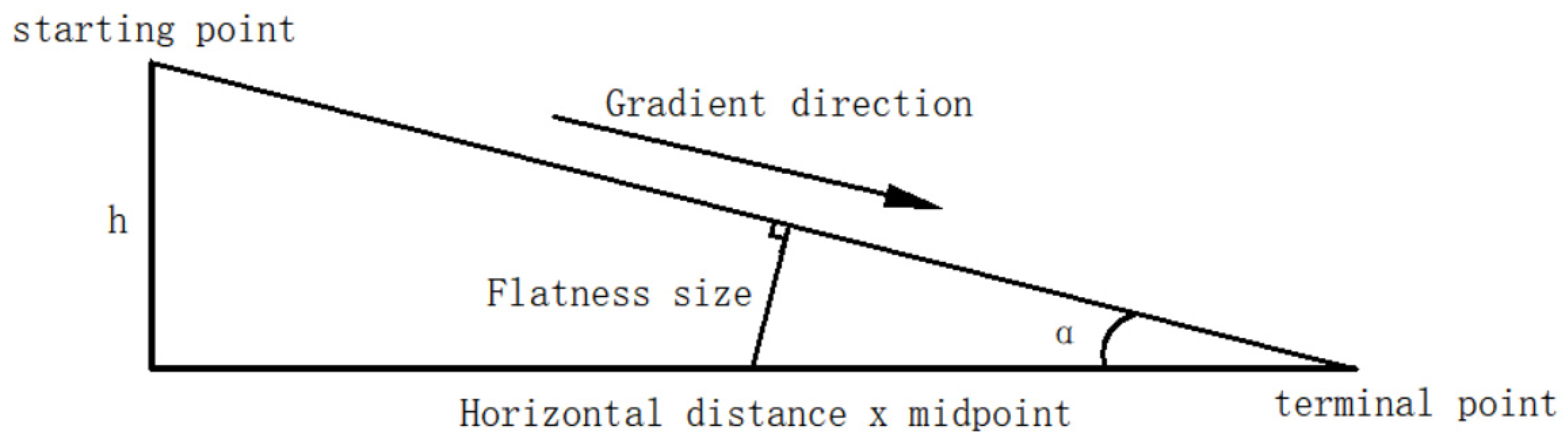
(6) To make the definition of local flatness meet the measurement requirements as much as possible and meet the technical specifications of tunnel engineering construction, the introduced three-dimensional laser scanning technology-based tunnel engineering primary surface flatness definition formula is as follows:

$$m_1=\frac{h\cos \alpha }{2}=\frac{x\sin \alpha }{2}=\frac{xh}{2\sqrt{h^2+x^2}}$$

(6)

In the formula, m₁ is the local flatness of the initial support surface of the tunnel, X represents the step distance of the original point cloud along the gradient direction, h represents the height difference between the starting point and the endpoint of the stepping direction, and $\alpha$ represents the inclination angle between the two points.

The schematic diagram of the local flatness definition is shown in Figure 13. The horizontal axis represents the direction of the horizontal step distance X, and the vertical axis represents the relative height h between the original point and the endpoint of the gradient direction.

4. Engineering Case Analysis

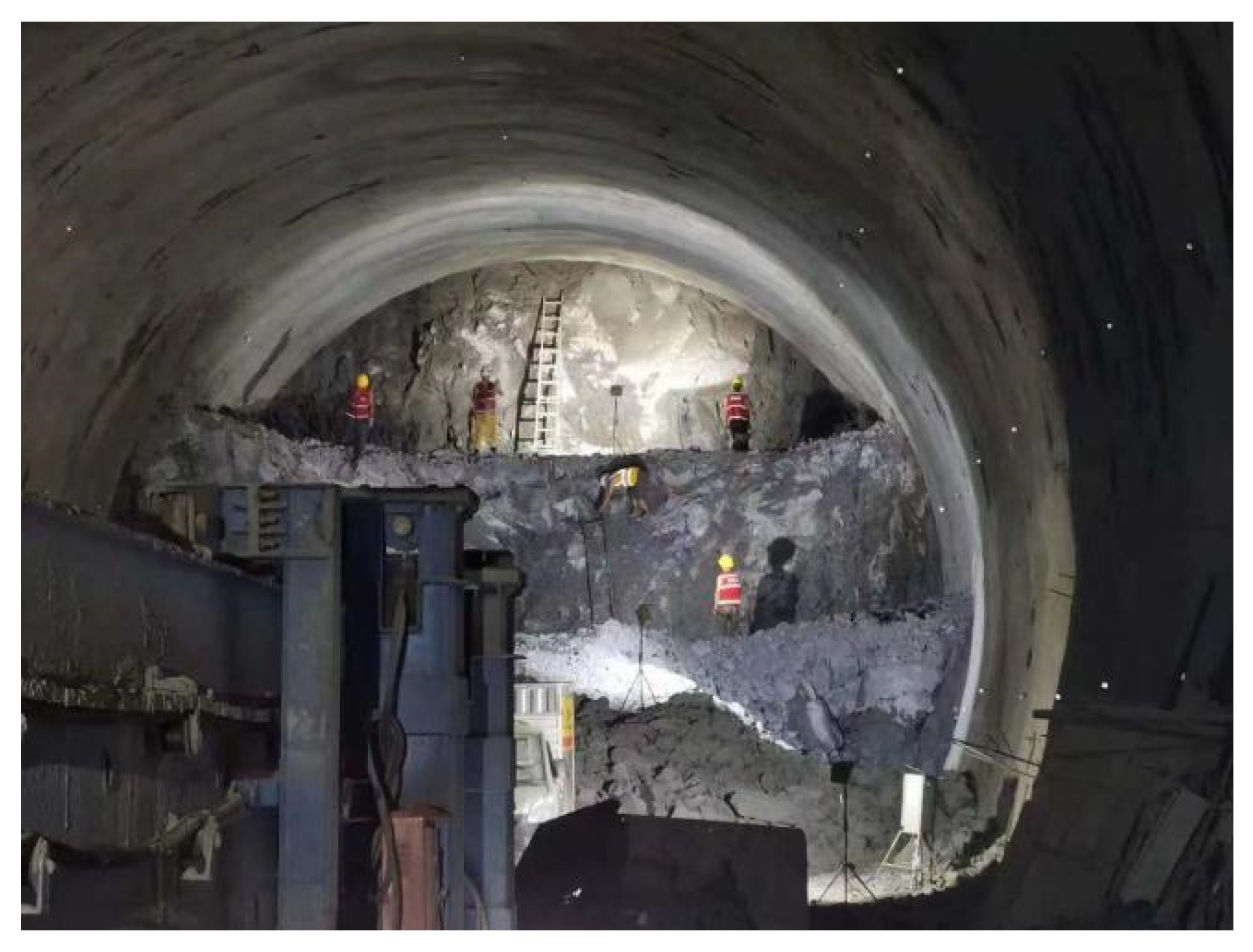
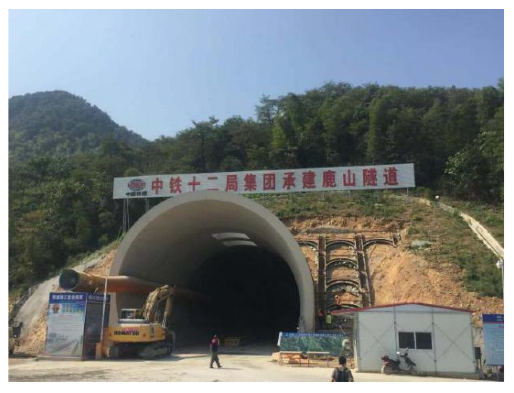
The project supported by this test is the Lushan Tunnel Project shown in Figure 14. The Lushan Tunnel is located in Fuyang, Hangzhou City, Zhejiang Province. It is a section of the newly-built Huhang Railway. The main surrounding rock grade is Grade V, and the area sections that need to collect point cloud data for flatness detection are mainly concentrated in the initial support section of the tunnel. A total of 30-m-long section areas are collected. The mileage section is DK109+870~DK109+900, whichever is selected The 2 m part is used as the analysis object of this experiment. The parameters of some regional sections of the Lushan Tunnel Project are shown in

Table 3. List of regional parameters of Lushan Tunnel.

Tunnel Name	Serial No.	Scope	Surrounding Rock Grade	Length (m)	Geological Condition
Lushan Tunnel	1	DK107+468~DK107+870	V	402	Inlet section, shallow buried section
	2	DK107+870~DK107+920	IV	50	sandstone
	3	DK107+920~DK108+715	III	795	sandstone
	4	DK108+715~DK108+770	IV	55	Shallow buried section
	5	DK108+770~DK109+570	V	800	Shallow buried section
	6	DK109+570~DK109+645	IV	75	Fault affected zone
	7	DK109+645~DK109+720	IV	75	Fault affected zone
	8	DK109+720~DK110+180	III	460	Feldspar quartz sand layer

.

The experiment uses a three-dimensional laser scanner to scan the surface of the initial support of the tunnel and collect the point cloud data of the surface of the initial support of the tunnel in a section of the area. After the point cloud data is preprocessed, the surface point cloud data of the initial support of the tunnel is curved and smoothed by the programming method to obtain the final flatness calculation datum. The normal vector distance is obtained according to the datum plane, to calculate and analyze the flatness of the initial support surface of the tunnel.

4.1. Analysis of Overall Flatness

In the experiment, the point cloud data of a 2-m-long tunnel surface cross-section was taken along the direction of the central axis of the tunnel. After preprocessing the point cloud data, a total of 40,000 points are selected by random sampling, and their normal vector distance is calculated, and a 200 × 200 normal vector distance scalar matrix is formed at the same time. Then, through the coordinates of the point cloud data, there are one-to-one correspondence in the X-axis central axis direction and the Y-axis cross-sectional direction. Finally, the normal vector distance scalar matrix is colored into a graph to analyze the overall flatness of the tunnel surface, as shown in Figure 15.

According to the calculation formula for the overall flatness of the surface of the initial support of the tunnel, the overall flatness of the surface of the first support of the tunnel is 19.9 mm. According to the “GB-T 50299-2018 Construction Quality Acceptance Standard for Underground Railway Engineering” [33], the flatness of the sprayed concrete is allowed the deviation should be 30 mm, and the overall flatness of the initial support surface of the tunnel meets the requirements of the specification.

4.2. Analysis of Local Flatness

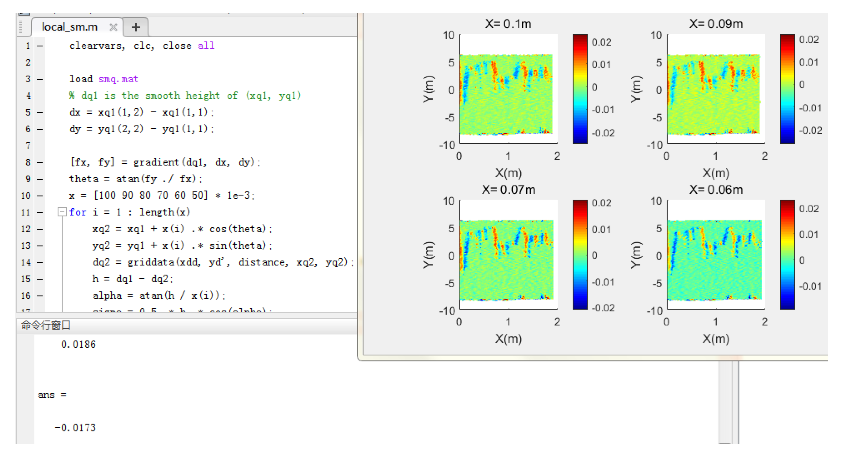
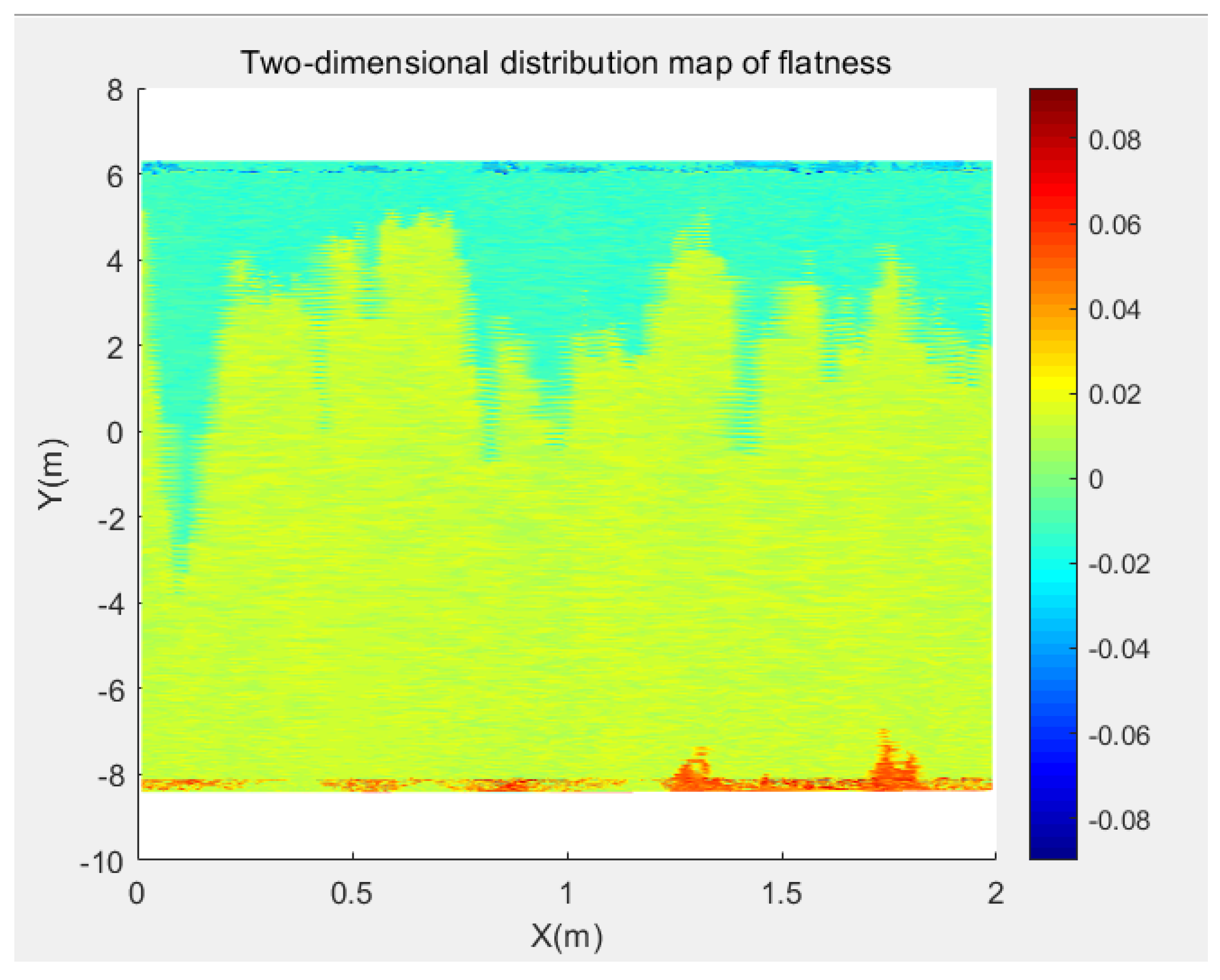
The analysis of local flatness first draws a flatness distribution map through the normal vector distance, and each point in the figure obtains the gradient of each point according to the gradient formula. In the gradient direction, the flatness changes the fastest. The local flatness is calculated in the gradient direction, and the local flatness is calculated and analyzed by determining the value of the horizontal distance X in the gradient direction. After the value of the horizontal distance X is determined, the height difference h between the starting point and the endpoint can be obtained, and X and h can be substituted into the local flatness calculation formula to obtain the final local flatness.

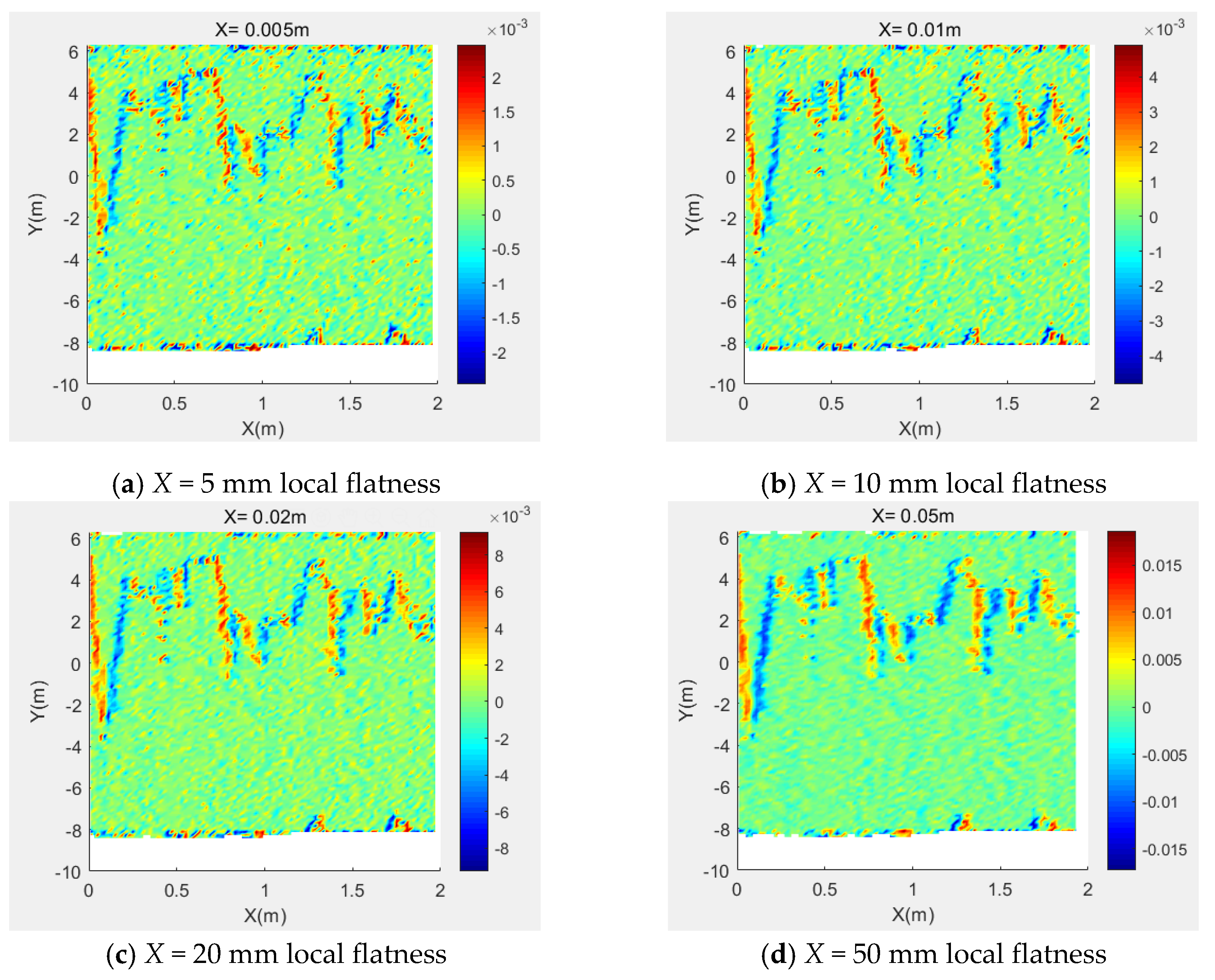
In this experiment, to analyze the influence of the value of the horizontal distance x on the local flatness results of the initial support surface of the tunnel, four-parameter values of X = 5 mm, X = 10 mm, X = 20 mm, and X = 50 mm were taken to determine the local flatness. The calculation and analysis of flatness are shown in Figure 16. In the figure, the X-axis is along the central axis of the tunnel, and the Y-axis is the direction of the cross-section of the tunnel.

Through the calculation of the local flatness of the initial support surface of the tunnel, when X = 5 mm, the maximum local flatness is 2.5 mm and the minimum is −2.5 mm; when X = 10 mm, the maximum local flatness is 4.9 mm and the minimum When X = 20 mm, the maximum local flatness is 9.3 mm and the minimum is −9.3 mm; when X = 50 mm, the local flatness maximum is 18.6 mm and the minimum is −17.3 mm.

The traditional flatness detection of the initial support of the tunnel is to detect the flatness of the initial support of the tunnel by a combination of a two-meter ruler and a wedge feeler. During the inspection, place the two-meter ruler horizontally on the tunnel surface along the direction of the central axis of the tunnel. The ruler is close to the tunnel surface and finds the largest gap. Place the wedge-shaped feeler gauge here. The reading is the ruler datum plane and the initial support of the tunnel. The maximum gap distance of the protective surface is the flatness of the initial support surface of the tunnel [34]. According to the “GB-T 50299-2018 Construction Quality Acceptance Standard for Underground Railway Engineering”, the allowable deviation of the flatness of the shotcrete should be 30 mm, and the local flatness of the initial support surface of the tunnel for the four sets of data meets the requirements of the specification.

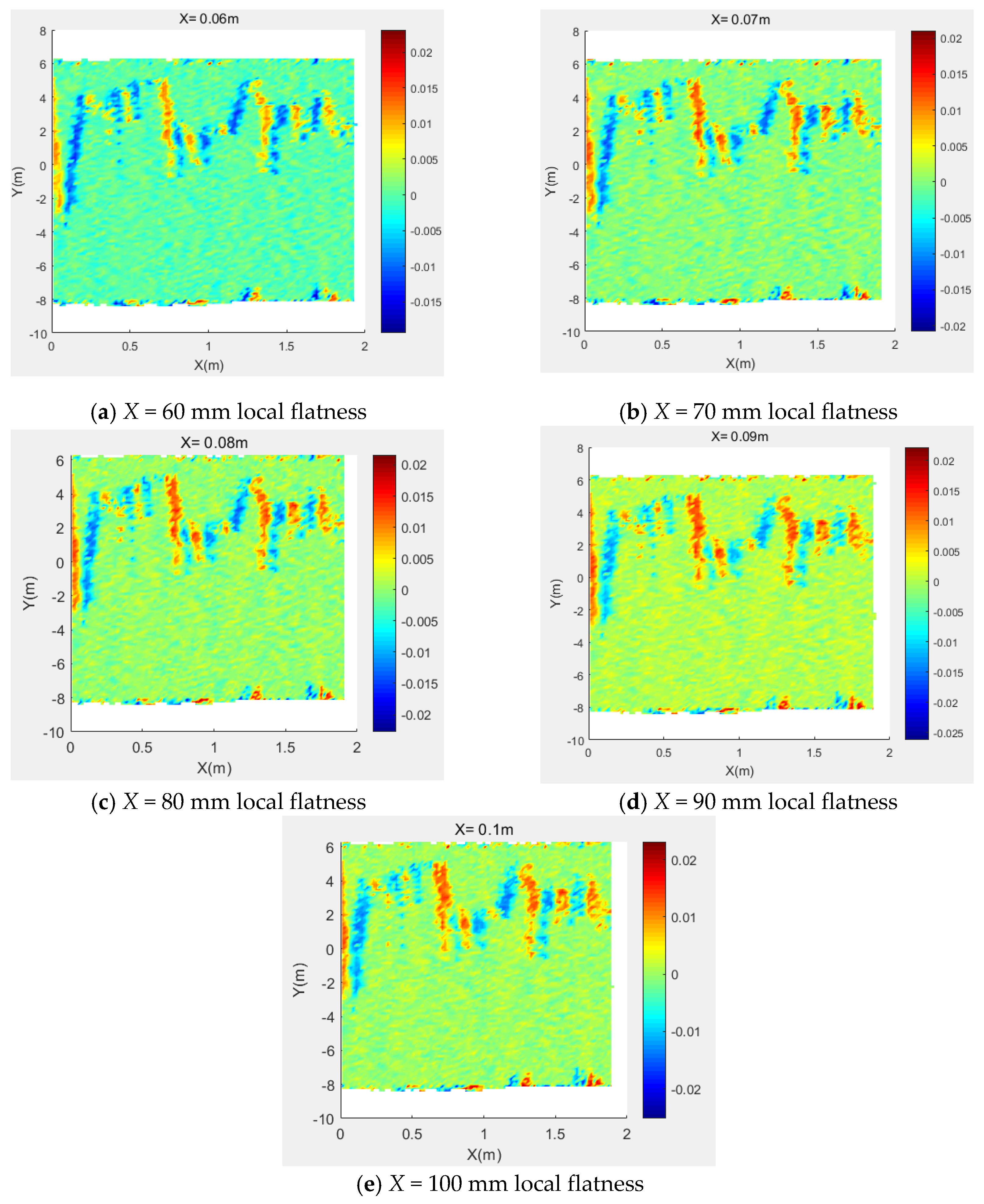
When the value of X gradually increases, the local flatness value of the initial support surface of the tunnel also gradually increases. At the same time, when the value of X gradually increases, the local flatness value also tends to stabilize. To further determine when the local flatness tends to be stable, this paper adds five sets of variable test data X = 60~100 mm, as shown in Figure 17. In the figure, the X-axis is along the central axis of the tunnel, and the Y-axis is the direction of the cross-section of the tunnel.

It can be seen from the two sets of test data that the horizontal distance X has a greater impact on the calculation of local flatness. The results of overall flatness and local flatness are summarized, as shown in

Table 4. Summarization of flatness calculation results.

	Max (mm)	Minimum (mm)	Abs Max (mm)
Overall flatness	19.9		19.9
Local flatness (X = 5 mm)	2.5	−2.5	2.5
Local flatness (X = 10 mm)	4.9	−4.8	4.9
Local flatness (X = 20 mm)	9.3	−9.3	9.3
Local flatness (X = 50 mm)	18.6	−17.3	18.6
Local flatness (X = 60 mm)	19.5	−19.4	19.5
Local flatness (X = 70 mm)	19.9	−20.0	20.0
Local flatness (X = 80 mm)	20.6	−20.8	20.8
Local flatness (X = 90 mm)	20.3	−20.6	20.6
Local flatness (X = 100 mm)	20.1	−20.3	20.3

below.

The following conclusions can be drawn from the analysis of the above table and the flatness distribution graph: (1) The calculation of local flatness depends on the program setting parameter step distance X. Choosing a suitable step distance parameter is very important for local flatness detection. When the value of X becomes larger and larger, the value of local flatness becomes larger and larger, and its value will approach the upper limit, which is similar to the calculation result of overall flatness. The approximate interval of the advance distance X is between 70 mm~90 mm, and it can be preliminarily judged that the Dangmai advance distance parameter setting between 70 mm~90 mm is suitable for local flatness detection. (2) By comparing and analyzing the flatness of the local flatness distribution map and the overall flatness distribution map, the flatness distributions of the two are basically the same. It can be explained that the detection methods of the overall flatness and the local flatness affect the flatness of the initial support of the tunnel. The representations are the same and the two have commonality. At the same time, the surface flatness of the initial support of the tunnel in this area meets the specification requirements. The local flatness calculation formula based on three-dimensional laser scanning proposed in this experiment is feasible.

4.3. Feasibility Analysis

To verify the effectiveness and feasibility of the method of detecting the surface flatness of the initial branch of the tunnel based on the 3DLS technology, this study compares and analyzes the point cloud data detected by the total station and the point cloud data detected by the 3DLS technology. The tunnel mileage K107+780, K107+785, K107+790, and K107+795 are, respectively, taken from four cross-section information, and each cross-section is taken from the left and right arch bottom, left and right arch waist, and the position of the archtop. The points were measured 4 times with a three-dimensional laser scanner at the same time interval. The thickness of the difference between the monitoring point and the design section collected by the total station is recorded as d₁, and the thickness of the difference between the monitoring point and the design section collected by 3DLS is recorded as d₂, and the statistical results of the test data collected by the two measuring instruments are summarized, as shown in

Table 5. Section monitoring point detection value.

Section Mileage Stake	Monitoring Points Position	Class 1 Detection Value d2/mm	Class 2 Detection Value d2/mm	Class 3 Detection Value d2/mm	Class 4 Detection Value d2/mm	Total Station Detection Value d1/mm
K107+780	Left arch	196	203	195	193	199
	Left arched waist	208	211	208	204	210
	dome	202	203	206	200	204
	Right arched waist	179	178	183	184	180
	Right arch	135	127	140	*	143
K107+785	Left arch	243	246	242	233	233
	Left arched waist	229	230	246	241	237
	dome	230	229	230	220	226
	Right arched waist	219	230	212	225	216
	Right arch	219	218	222	*	225
K107+790	Left arch	184	190	160	176	171
	Left arched waist	247	268	247	245	237
	dome	209	229	216	212	212
	Right arched waist	216	214	208	202	213
	Right arch	176	177	173	*	174
K107+795	Left arch	239	258	236	*	224
	Left arched waist	274	266	265	260	257
	dome	244	249	244	242	232
	Right arched waist	200	218	204	214	194
	Right arch	191	201	*	*	183

Note: * indicates that the location is blocked, and the data at this point has not been measured.

below.

It can be seen from the data in the tab that the detection value collected by 3DLS is roughly the same as the detection value collected by the total station. To further illustrate the accuracy and effectiveness of the flatness detection method based on the 3DLS technology, this study will the detection value of the total station is regarded as the most reliable value $\widehat{x}$. and the detection value of the scanner is regarded as the observation value x_i. The detection difference $\Delta d$ of 4 tests can be calculated respectively, and finally the median error $\widehat{\sigma }$ of 3DLS can be calculated by the detection difference $\Delta d$. The error $\widehat{\sigma }$ in the calculated observation value can represent the true error of 3DLS. The Medium error result is shown in

Table 6. The two instruments measure the difference.

Section Mileage Stake	Distance to Station/m	Monitoring Points Position	Class 1 $\mathbf{Difference}\mathbf{\Delta }\mathit{d}/\mathbf{mm}$	Class 2 $\mathbf{Difference}\mathbf{\Delta }\mathit{d}/\mathbf{mm}$	Class 3 $\mathbf{Difference}\mathbf{\Delta }\mathit{d}/\mathbf{mm}$	Class 4 $\mathbf{Difference}\mathbf{\Delta }\mathit{d}/\mathbf{mm}$
K107+780		Left arch	3	4	4	6
		Left arched waist	2	1	2	6
	0	dome	2	1	2	4
		Right arched waist	1	2	3	4
		Right arch	8	16	3	*
Medium error $\widehat{\sigma }$			5	8	3	6
K107+785		Left arch	10	13	9	0
		Left arched waist	8	7	9	4
	5	dome	4	3	4	6
		Right arched waist	3	14	4	9
		Right arch	6	7	3	*
Medium error $\widehat{\sigma }$			8	11	7	7
K107+790		Left arch	13	19	11	5
		Left arched waist	10	31	10	8
	10	dome	3	17	4	0
		Right arched waist	3	1	5	11
		Right arch	2	3	1	*
Medium error $\widehat{\sigma }$			9	20	8	8
K107+795		Left arch	15	34	12	*
		Left arched waist	7	9	8	3
	15	dome	12	17	12	10
		Right arched waist	6	24	10	20
		Right arch	8	18	*	*
Medium error $\widehat{\sigma }$			14	25	12	16

Note: * indicates that the location is blocked, and the data at this point has not been measured.

.

It can be seen from Table.6 that the true error of the 3DLS will increase as the distance between the section and the station increases. The cross-sectional instrument method, total station coordinate method or 3DLS method can be used, and the error in the measurement should not be greater than 25 mm [35]. Because the selection of the initial section of the tunnel in this study is a cross-sectional area of 2 m in the direction of the central axis By default, the center position of the cross-sectional area is the position of the measuring station, so the distance between the instrument and the scanned cross-section has little effect on the flatness detection results of this study. The true error of the 3DLS meets the requirements of the specification within a certain measurement range. The accuracy of the point cloud data collected by the 3DLS is improved.

5. Conclusions

This paper is based on the three-dimensional laser scanning technology to obtain the point cloud data of the initial support surface of the railway tunnel, and expounds the use of the tunnel point cloud data, through the B-spline interpolation method and the S-G smoothing method based on the curvature limitation, to obtain the flatness calculation reference plane. The normal vector distance formed by the intersection of the normal line drawn from the original point cloud and the flatness calculation datum plane is proposed, and the normal vector distance is used as the basis for flatness calculation, and two concepts based on the detection of the surface flatness of the initial support of the tunnel are introduced: the whole Flatness and local flatness. Through the analysis of the flatness distribution map and the flatness calculation results, the feasibility of the application of the three-dimensional laser scanning technology in the surface flatness detection of the initial support of the tunnel engineering is verified and discussed. The main conclusions are as follows:

(1) Compared with the traditional total station method and the two-meter ruler method in the traditional flatness detection, the efficiency is low, the accuracy is not high, and the operation is inconvenient. The use of three-dimensional laser scanning technology to detect the surface flatness of the initial support of the tunnel can quickly and accurately obtain the tunnel. A large amount of point cloud data on the surface of the initial support is easy to operate, without touching the surface of the initial support of the tunnel to be tested, and the accuracy of the instrument is high enough to make up for the problem of acquisition accuracy.

(2) Common surface fitting methods include meshing method, Poisson surface reconstruction method, Lagrangian interpolation method, and cubic B-spline interpolation method. To obtain the most suitable surface fitting method for this experiment, the experiment compares and analyzes the surface fitting degree and fitting accuracy of the four surface fitting methods. According to the comparative analysis, compared with the other three surface fitting methods, the tunnel surface constructed by the cubic B-spline interpolation method is continuous and complete, with higher smoothness, no local mutations, etc., and the details of the local area are rich and relatively The tunnel surface is restored well. At the same time, by calculating the statistical root mean square error of the four fitting methods, the fitting error of the surface area other than the original point can be obtained. The calculation result can be obtained by using the Poisson reconstruction method and the cubic B-spline interpolation method. The point cloud fitting error can be kept within a small range, and the fitting accuracy is high. Comprehensive comparative analysis shows that cubic B-spline interpolation is the most suitable fitting method for this study.

(3) After comparative analysis, a suitable surface fitting method for this experiment, namely cubic B-spline interpolation, has been obtained. On this basis, this research puts forward the method of two-way slice complementarity in the B-spline interpolation method to fit the overall surface of the tunnel and the method of SG filter smoothing based on curvature, which effectively eliminates the one-way slice to fit the whole tunnel. The jagged layering effect of the curved surface optimizes the fitting process of the tunnel curved surface. The optimized fitting surface is continuous and complete, with high smoothness, rich and complete local details, which is consistent with the actual engineering situation, and better restores the tunnel surface. At the same time, it can also meet the requirements of the flatness calculation of the initial support of the tunnel. It can be used as a reference plane for flatness calculation.

(4) The intersection of the normal line drawn from the original point cloud and the flatness calculation datum forms the normal vector distance. Based on this, this research proposes two flatness calculation methods and draws the flatness distribution map. The calculation of overall flatness can determine the overall flatness of the initial support surface of the tunnel, and the calculation of local flatness can determine the specific location of the uneven area. Combined with the flatness distribution map, the flatness detection can be more accurate and intuitive, which can be used for tunnel engineering. The construction provides technical support and theoretical guidance.

(5) In the flatness calculation method, this research proposes a local flatness calculation method. The step distance X set by the program is the main factor affecting the local flatness. In the flatness detection of the actual tunnel engineering, it is necessary to set an appropriate stepping distance X according to actual engineering conditions. To explore and analyze the influence of step distance X on local flatness, this study set up experimental groups with different step distance X to conduct analysis. The results show that the local flatness will increase as the step distance X increases. Finally, Infinite approaches the upper limit, which is roughly stable at around 20 mm, which is roughly the same as the overall flatness calculation result. According to the analysis of the flatness distribution map obtained by the two flatness calculation methods, the flatness of the initial tunnel support surface is basically consistent, which proves that the tunnel flatness detection method proposed in this study is feasible.

(6) Through the comparative analysis with the traditional flatness detection method, the true error of 3DLS meets the specification requirements within a certain measurement range, and both are less than the 25 mm required by the specification. This shows the accuracy of the point cloud data collected by 3DLS. At the same time, the initial fitting surface fitting of the tunnel project obtained by 3DLS technology has a higher degree of optimization and is closer to the actual engineering situation. The flatness calculation method is simpler and more effective, and the flatness analysis based on the flatness distribution map is more Precise and intuitive. The method of detecting the flatness of the initial support surface of the tunnel based on the three-dimensional laser scanning technology is feasible.

In summary, compared with traditional detection methods, 3DLS are faster and more accurate, with high acquisition accuracy, wide range, and simple operation in the detection of the flatness of the initial support surface of the tunnel. The surface fitting effect is best after cubic B-spline interpolation and SG filter smoothing based on curvature limitation. In this study, the normal vector distance is formed by the intersection of the normal line drawn from the original point cloud and the flatness calculation datum surface, and based on this, the concepts of overall flatness and local flatness are proposed, and corresponding flatness distribution maps are drawn respectively. The size of the local flatness will increase as the step distance X becomes larger, and finally, approach the calculation result of the overall flatness infinitely. Comparing the measurement accuracy of 3DLS and the traditional detection instrument, and comparing the flatness distribution map and the calculation results, it can be preliminarily concluded that the tunnel flatness detection method proposed in this study is feasible.

6. Outlook

The flatness detection method in this study is mainly for curved surfaces similar to the tunnel surface. For the traditional flatness detection methods, flatness detection can only be performed on relatively flat road surfaces or building walls. Through the research of the flatness detection method in this experiment, the purpose of flatness detection on a complex curved surface is realized. However, there are still some shortcomings in the research process:

(1) Obtaining the flatness calculation datum plane in the tunnel flatness detection calculation is a key step in calculating the flatness of the initial support of the tunnel, but how to determine that the flatness calculation datum obtained by processing is the most suitable and optimal solution flatness calculation datum plane, its treatment method is still worthy of further study.

(2) At this stage, there is no system for systematic evaluation of the flatness detection of the initial branches of the tunnel using 3DLS technology, so the construction of a more complete 3DLS tunnel flatness detection and evaluation system is the next research direction.