A New Linear Regression Kalman Filter with Symmetric Samples

Abstract

Nonlinear filtering is of great significance in industries. In this work, we develop a new linear regression Kalman filter for discrete nonlinear filtering problems. Under the framework of linear regression Kalman filter, the key step is minimizing the Kullback–Leibler divergence between standard normal distribution and its Dirac mixture approximation formed by symmetric samples so that we can obtain a set of samples which can capture the information of reference density. The samples representing the conditional densities evolve in a deterministic way, and therefore we need less samples compared with particle filter, as there is less variance in our method. The numerical results show that the new algorithm is more efficient compared with the widely used extended Kalman filter, unscented Kalman filter and particle filter.

1. Introduction

We aim to seek the optimal estimate of the state based on noisy observations in nonlinear filtering problems, which have a long history that can be traced back to the 1960s. In 1960, Kalman proposed the famous Kalman filter (KF) [1] and one year later, Kalman and Bucy proposed the Kalman–Bucy filter [2]. However, we need to assume that the filtering system is linear and Gaussian in KF. For general nonlinear filtering problems, we usually cannot obtain the optimal estimates. Therefore, approximations are required in order to derive suboptimal but still efficient estimators.

One direction is to approximate the nonlinear system. For instance, we approximate the original system by linear system using first-order Taylor expansions in the extended Kalman filter (EKF) [3]. Second-order variants of EKF can be found in [4]. In [5], the state is extended and then the nonlinear system is approximated by bilinear system using Carleman approach. Obviously, in these methods, the continuity of the system is required, and the estimations are sensitive to the specific point used for the expansion.

Instead, we can approximate the conditional density function rather than the system, since the optimal estimate is completely determined by the conditional density. For example, in particle filter (PF) [6] and its variants, we use the empirical distribution of some particles to approximate the real conditional distribution. For continuous filtering systems, the posterior density function satisfies the Duncan–Mortensen–Zakai equation [7,8,9] and there are many works aiming to solve this equation such as the direct method [10] and Yau–Yau method [11,12,13].

If we approximate the conditional density by single Gaussian distribution, and use KF formulas in updating step, then we can obtain a class of the so-called Nonlinear Kalman Filters [4]. However, we still need linearization in case of nonlinear systems, and one suitable way to perform such linearization is statistical linearization in the form of statistical linear regression [14]. In this sample-based approach, we represent the related densities by a set of random or deterministic selected samples. The class of Nonlinear Kalman Filters which make use of statistical linear regression are called Linear Regression Kalman Filters (LRKFs) [14]. For more details about LRKF, readers are referred to the work in [15]. The unscented Kalman filter (UKF) [16] is the most commonly used LRKF, which use a fixed number of deterministic sigma-points to capture the information of the conditional densities. Intuitively, the LRKF can be viewed as a hybrid of PF and KF, where the particles are obtained in a deterministic way. There are some heuristic algorithms that combine PF and KF directly in many practical applications such as target tracking [17,18].

The key problem in LRKF is how to select the points, which can be determined by minimizing some distance between original density and its Dirac mixture density formed by these points. In this paper, we propose a new LRKF which uses Kullback–Leibler (K-L) divergence as the measure. Motivated by the work [19] and considering the symmetry of Gaussian distribution, we approximate the standard normal density by the Dirac mixture density formed by any given number of symmetric points. Now, we only need to solve a optimization problem. There are many PFs based on MCMC sampling in recent decades. However, only a few papers have improved particle sampling by variational inference, as it is difficult to calculate the K-L divergence between discrete densities. With the rise of a large number of generative models in machine learning, more and more approximate algorithms related to variational inference are produced, and Stein variational gradient decent (SVGD) is an important one [20,21]. SVGD drives the discrete particles to approximate the continuous posterior density function by kernel functions, so that the K-L divergence between the continuous density and its Dirac mixture approximation by discrete points is minimized by using gradient descent. We then obtain the points which can approximate non-standard Gaussian density functions by Mahalanobis transformation [22]. At last, using the framework of LRKF, we can obtain the estimation result. Inheriting the advantages of LRKF, we can handle discontinuous filtering systems by the proposed algorithm and we do not need to compute the Jacobian matrix.

The first contribution of this work is that we introduce K–L divergence to measure the distance of the continuous density and its Dirac mixture approximation formed by any given number of symmetric samples. Besides, we use SVGD to solve the corresponding optimization problem motivated by frequently uses of variational inference in machine learning. It can be seen from the numerical simulations that our algorithm shows great efficiency compared with classical EKF, UKF, and PF.

Notations: $\left|·\right|$ represents the Euclidean norm. $\delta (·)$ denotes the Dirac delta function, i.e.,

$$\delta \left(x\right)=\left\{\begin{array}{ccc}\hfill & +\infty \hfill & \hfill x=0,\\ \hfill & 0\hfill & \hfill x\ne 0,\end{array}\right.$$

which is also constrained to satisfy the identity

$${\int }_{-\infty }^{\infty }\delta \left(x\right)=1.$$

$\mathcal{N}(x;m,P)$ denotes the Gaussian density function with mean m and positive definite covariance P, i.e.,

$$\mathcal{N}(x;m,P)={\displaystyle \frac{1}{\sqrt{{\left(2\pi \right)}^n\det P}}}exp\left(-{\displaystyle \frac{1}{2}}{(x-m)}^{\mathrm{T}}{P}^{-1}(x-m)\right),$$

where n is the dimension of x and $\det P$ is the determinant of P.

This paper is organized as follows. In Section 2, we review the basic filtering problem and some preliminary results. In Section 3, we give one new LRKF. In  Section 4, a numerical example is implemented to show the efficiency of the new algorithm.

2. Preliminaries

The discrete time filtering system considered here is as follows:

$$\begin{array}{cc}\hfill x_k& =a_k(x_{k-1},w_k),\hfill \end{array}$$

(1)

$$\begin{array}{cc}\hfill y_k& =h_k(x_k,v_k),\hfill \end{array}$$

(2)

where $x_k\in {\mathbb{R}}^n$ is the state of the stochastic nonlinear dynamic system (1) at discrete time instant k, $y_k\in {\mathbb{R}}^m$ is the noisy measurement (or observation) generated according to the model (), and $\{w_k\in {\mathbb{R}}^q,k=0,1,\cdots \}$ and $\{v_k\in {\mathbb{R}}^r,k=1,\cdots \}$ are Gaussian white noise processes with $w_k\sim \mathcal{N}(w_k;0,Q_k)$ and $v_k\sim \mathcal{N}(v_k;0,R_k)$. Here we need to assume that $\{w_k,k=0,1,\cdots \}$, $\{v_k,k=1,\cdots \}$ and the initial state $x_0$ are independent of each other. The density function of the initial state $x_0$ is $p\left(x_0\right)$. $Y_k$ denotes the history of the observations up to time instant k, i.e.,

$$Y_k:=\{y_1,\cdots ,y_k\}.$$

(3)

We aim to seek the optimal estimate of state $x_k$ based on the observation history $Y_k$ in the sense of minimum mean square error.

Definition 1 (Minimum mean square error estimate([3])). Let $\widehat{x}$ be an estimate of random variable x. Then the minimum mean square error estimate of x is

$$\underset{\widehat{x}}{argmin}\mathbb{E}\left[{(x-\widehat{x})}^{\mathrm{T}}(x-\widehat{x})\right].$$

Jazwinski proved that the minimum mean square error estimate of state $x_k$ based on $Y_k$ is its conditional expectation in the following theorem.

Theorem 1

(Theorem 5.3 in [3]). Let the estimate of $x_k$ be a functional on $Y_k$. Then, the minimum mean square error estimate of state $x_k$ is its conditional mean $\mathbb{E}\left[x_k\right|Y_k]$.

Obviously, if we can obtain the conditional density of $x_k$ based on $Y_k$, i.e., $p\left(x_k\right|Y_k)$, then we can simply compute $\mathbb{E}\left[x_k\right|Y_k]$. The evolution of the conditional density function $p\left(x_k\right|Y_k)$ is given in the following theorem.

Theorem 2

([19]). Consider the filtering problem (1)–() from time step $k-1$ to step k. The evolution of the conditional density function $p\left(x_k\right|Y_k)$ contains iterative two steps:

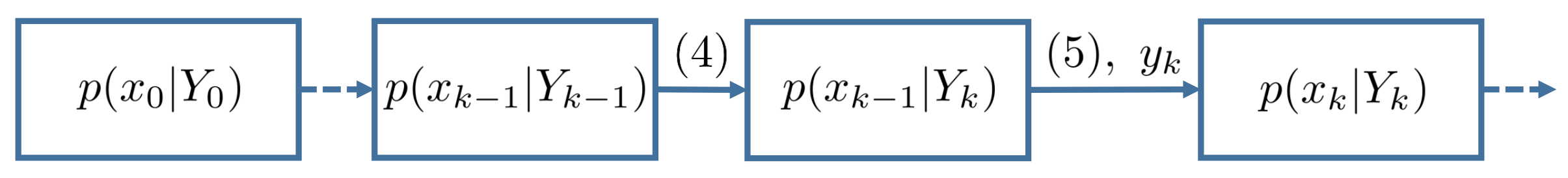
• In the prediction step, employing the system model (1) and the Chapman–Kolomogorov equation, we can obtain

  $$\begin{array}{cc}\hfill p\left(x_k\right|Y_{k-1})& =\int p\left(x_k\right|x_{k-1})·p\left(x_{k-1}\right|Y_{k-1})\hfill \\ \hfill & =\int \int \delta (x_k-a_k(x_{k-1},w_k))·p\left(x_{k-1}\right|Y_{k-1})·p\left(w_k\right)d{x}_{k-1}d{w}_k,\hfill \end{array}$$

  (4)
  where

  $$p\left(w_k\right)=\mathcal{N}(w_k;0,Q_k).$$
• In the updating step, when the latest measurement $y_k$ arrives, using Bayes’ rule, we have

  $$\begin{array}{c}\hfill p\left(x_k\right|Y_k)={\displaystyle \frac{p\left(y_k\right|x_k)·p\left(x_k\right|Y_{k-1})}{p\left(y_k\right|Y_{k-1})}},\end{array}$$

  (5)
  where the likelihood function $p\left(y_k\right|x_k)$ is obtained according to

  $$p\left(y_k\right|x_k)=\int \delta (y_k-h_k(x_k,v_k))·p\left(v_k\right)d{v}_k,$$

  (6)
  with

  $$p\left(v_k\right)=\mathcal{N}(v_k;0,R_k).$$

The initial value of the conditional density function is $p\left(x_0\right|Y_0)=p\left(x_0\right)$. Then according to Theorem 2, we have the evolution framework of $p\left(x_k\right|Y_k)$ which is shown in the following Figure 1.

Figure 1. The evolutions of the posterior density functions.

Unfortunately, we cannot obtain the conditional density function analytically in most cases, although we have the recursive evolution equations of conditional density functions. Therefore, we cannot get the optimal estimate $\mathbb{E}\left[x_k\right|Y_k]$, and we need to resort to some approximation techniques.

2.1. Nonlinear Kalman Filtering Based on Statistical Linearization

One important approximative Bayesian estimation technique is used in the class of Nonlinear Kalman Filter. These filters assume that both $p\left(x_k\right|Y_{k-1})$ and $p\left(x_k\right|Y_k)$ are well approximated by Gaussian distributions. The detailed procedures are listed as follows [19].

1.

Initialization: The initial density of $x_0$ is approximated by Gaussian:

$$p\left(x_0\right)\approx \mathcal{N}(x_0;{\widehat{x}}_{0|0},{\mathbf{P}}_{0|0})$$

(7)

with the initial mean

$${\widehat{x}}_{0|0}:=\int x_{0}p\left(x_0\right)d{x}_0$$

(8)

and initial covariance

$${\mathbf{P}}_{0|0}:=\int \left(x_0-{\widehat{x}}_{0|0}\right){\left(x_0-{\widehat{x}}_{0|0}\right)}^{\mathrm{T}}p\left(x_0\right)d{x}_0.$$

(9)

2.

Prediction: The apriori density function is approximated by

$$p\left(x_k\right|Y_{k-1})\approx \mathcal{N}(x_k;{\widehat{x}}_{k|k-1},{\mathbf{P}}_{k|k-1}),$$

(10)

with predicted state mean

$$\begin{array}{cc}\hfill {\widehat{x}}_{k|k-1}:=& \int x_{k}p\left(x_k\right|Y_{k-1})d{x}_k\hfill \\ \hfill =& \int \int a_k(x_{k-1},w_k)·p\left(x_{k-1}\right|Y_{k-1})·p\left(w_k\right)d{x}_{k-1}d{w}_k\hfill \end{array}$$

(11)

and predicted state covariance matrix

$$\begin{array}{cc}\hfill {\mathbf{P}}_{k|k-1}:=& \int (x_k-{\widehat{x}}_{k|k-1}){(x_k-{\widehat{x}}_{k|k-1})}^{\mathrm{T}}p\left(x_k\right|Y_{k-1})d{x}_k\hfill \\ \hfill =& \int \int (a_k(x_{k-1},w_k)-{\widehat{x}}_{k|k-1}){(a_k(x_{k-1},w_k)-{\widehat{x}}_{k|k-1})}^{\mathrm{T}}\hfill \\ \hfill & ·p\left(x_{k-1}\right|Y_{k-1})·p\left(w_k\right)d{x}_{k-1}d{w}_k,\hfill \end{array}$$

(12)

respectively.

3.

Updating: The Bayesian filter step (5) can be reformulated in form of the joint density $p(x_k,y_k|Y_{k-1})$ according to

$$p\left(x_k\right|Y_k)={\displaystyle \frac{p(x_k,y_k|Y_{k-1})}{p\left(y_k\right|Y_{k-1})}}.$$

(13)

Here, this joint density is approximated by Gaussian

$$p\left(x_k\right|Y_k)\approx \frac{\mathcal{N}\left(\left[\begin{array}{c}{x}_k\\ y_k\end{array}\right];\left[\begin{array}{c}{\widehat{x}}_{k|k-1}\\ {\widehat{y}}_k\end{array}\right],\left[\begin{array}{cc}{\mathbf{P}}_{k|k-1}& {\mathbf{P}}_k^{x,y}\\ {\left({\mathbf{P}}_k^{x,y}\right)}^{\mathrm{T}}& {\mathbf{P}}_k^y\end{array}\right]\right)}{p\left(y_k\right|Y_{k-1})}=\mathcal{N}\left(x_k;{\widehat{x}}_{k|k},{\mathbf{P}}_{k|k}\right),$$

(14)

then according to Theorem A2 in Appendix A, posterior state mean

$${\widehat{x}}_{k|k}={\widehat{x}}_{k|k-1}+{\mathbf{P}}_k^{x,y}·{\left({\mathbf{P}}_k^y\right)}^{-1}·\left(y_k-{\widehat{y}}_k\right),$$

(15)

and posterior state covariance matrix

$${\mathbf{P}}_{k|k}={\mathbf{P}}_{k|k-1}-{\mathbf{P}}_k^{x,y}·{\left({\mathbf{P}}_k^y\right)}^{-1}·{\left({\mathbf{P}}_k^{x,y}\right)}^{\mathrm{T}},$$

(16)

where the measurement mean

$$\begin{array}{cc}\hfill {\widehat{y}}_k& =\int y_k·p\left(y_k\right|Y_{k-1})\mathrm{d}{y}_k\hfill \\ \hfill & =\int \int h_k\left(x_k,v_k\right)·p\left(x_k\right|Y_{k-1})·p\left(v_k\right)\mathrm{d}{x}_k\mathrm{d}{v}_k,\hfill \end{array}$$

(17)

the measurement covariance matrix

$$\begin{array}{cc}\hfill {\mathbf{P}}_k^y& =\int \left(y_k-{\widehat{y}}_k\right)·{\left(y_k-{\widehat{y}}_k\right)}^{\mathrm{T}}·p\left(y_k\right|Y_{k-1})\mathrm{d}{y}_k\hfill \\ \hfill & =\int \int \left(h_k\left(x_k,v_k\right)-{\widehat{y}}_k\right)·{\left(h_k\left(x_k,v_k\right)-{\widehat{y}}_k\right)}^{\mathrm{T}}·p\left(x_k\right|Y_{k-1})·p\left(v_k\right)\mathrm{d}{x}_k\mathrm{d}{v}_k,\hfill \end{array}$$

(18)

as well as the cross-covariance matrix of predicted state and measurement

$$\begin{array}{cc}\hfill {\mathbf{P}}_k^{x,y}& =\int \int \left(x_k-{\widehat{x}}_{k|k-1}\right)·{\left(y_k-{\widehat{y}}_k\right)}^{\mathrm{T}}·p(x_k,y_k|Y_{k-1})\mathrm{d}{x}_k\mathrm{d}{y}_k\hfill \\ \hfill & =\int \int \left(x_k-{\widehat{x}}_{k|k-1}\right)·{\left(h_k\left(x_k,v_k\right)-{\widehat{y}}_k\right)}^{\mathrm{T}}·p\left(x_k\right|Y_{k-1})·p\left(v_k\right)\mathrm{d}{x}_k\mathrm{d}{v}_k.\hfill \end{array}$$

(19)

However, we cannot obtain the closed form integrals in the above equations in general cases.

2.2. The Linear Regression Kalman Filter

If the state densities in the integrals of the Nonlinear Kalman Filter can be replaced by proper Dirac mixture densities formed by some samples, then we can easily compute these integrals. That is, the statistical linearization is turned into an approximate statistical linear regression, and this is exactly what the LRKF does.

The Dirac mixture approximation of an arbitrary density $p\left(s_k\right)$ of $s_k\in {\mathbb{R}}^N$ by L samples is

$$p\left(s_k\right)\approx {\tilde{p}}^L\left(s_k\right):=\sum _{i=1}^L{\alpha }_{k,i}·\delta (s_k-s_{k,i})$$

(20)

with samples $\{s_{k,1},\cdots ,s_{k,L}\}$ and positive scalar weights $\{{\alpha }_{k,1},\cdots ,{\alpha }_{k,L}\}$, for which

$$\sum _{i=1}^L{\alpha }_{k,i}=1.$$

(21)

Therefore, the information of the density $p\left(s_k\right)$ is approximately encoded in the $L(N+1)$ Dirac mixture parameters, which can be determined by minimizing certain distance between $p\left(s_k\right)$ and ${\tilde{p}}^L\left(s_k\right)$.

2.3. The Smart Sampling Kalman Filter

One of the LRKFs is the smart sampling Kalman Filter proposed in [15]. As the goal in LRKF is to approximate Gaussian densities $p\left(x_k\right|Y_{k-1})$ and $p\left(x_k\right|Y_k)$ by Dirac mixture densities, They first consider to approximate an N-dimensional standard normal distribution $\mathcal{N}(s;0,\mathbf{I})$ by Dirac mixture approximation using equal weights and symmetric samples in the following manner:

$$\begin{array}{cc}\hfill & \mathcal{N}(s;0,\mathbf{I})\approx \frac{1}{2L}\sum _{i=1}^L\delta \left(s-s_i\right)+\delta \left(s+s_i\right),\mathrm{even}\mathrm{number}\mathrm{of}\mathrm{samples};\hfill \\ \hfill & \mathcal{N}(s;0,\mathbf{I})\approx \frac{1}{2L+1}\left(\delta \left(s\right)+\sum _{i=1}^L\delta \left(s-s_i\right)+\delta \left(s+s_i\right)\right),\mathrm{odd}\mathrm{number}\mathrm{of}\mathrm{samples}.\hfill \end{array}$$

(22)

Then, given a non-standard Gaussian distribution

$$\mathcal{N}(z;m_z,P_z),$$

(23)

we can use the Mahalanobis transformation [22] to obtain the Dirac mixture approximation. More explicitly, by transforming the samples $s_i$ in (22) according to

$$\begin{array}{cc}\hfill z_i& =\sqrt{P_z}·s_i+m_z,\forall 1\le i\le L,\hfill \\ \hfill z_i& =-\sqrt{P_z}·s_{i-L}+m_z,\forall L+1\le i\le 2L,\hfill \end{array}$$

(24)

where $\sqrt{P_z}$ is the square root of $P_z$ using Cholesky decomposition, we have the Dirac mixture approximation of (23) as follows:

$$\begin{array}{cc}\hfill & \mathcal{N}(z;m_z,P_z)\approx \frac{1}{2L}\sum _{i=1}^{2L}\delta \left(z-z_i\right),\mathrm{even}\mathrm{number}\mathrm{of}\mathrm{samples};\hfill \\ \hfill & \mathcal{N}(z;m_z,P_z)\approx \frac{1}{2L+1}\left(\delta (z-m_z)+\sum _{i=1}^{2L}\delta \left(z-z_i\right)\right),\mathrm{odd}\mathrm{number}\mathrm{of}\mathrm{samples}.\hfill \end{array}$$

(25)

Moreover, this transformation can be also understood from the property of Gaussian random variables listed in Theorem A1.

By approximating the approximated a priori density $\mathcal{N}(x_k;{\widehat{x}}_{k|k-1},{\mathbf{P}}_{k|k-1})$ in (10) and posterior density $\mathcal{N}(x_k;{\widehat{x}}_{k|k},{\mathbf{P}}_{k|k})$ in (14) using (24) and (25), we can get the desired filtering result under the framework of LRKF. Now the key is how to determine the samples $\{s_1,\cdots ,s_L\}$ in (22) so that they approximate a multivariate standard normal distribution in an optimal way. In [19], a combination of the Localized Cumulative Distribution and the modified Cramér–von Mises distance is adapted.

3. The New Linear Regression Kalman Filter

Apparently, in the framework of LRKF, we need to approach the goal through the formulation of an optimization problem with respect to the appropriate chosen distance metric between original density and its Dirac mixture approximation. Instead of the distance measure adapted in [19], we can minimize the K–L divergence between the multivariate standard normal distribution $\mathcal{N}(s;0,I_n)\triangleq p_{\mathrm{N}}\left(s\right)$ and its approximation

$${\tilde{p}}_{\mathrm{N}}\left(s\right):=\frac{1}{2L}\left(\sum _{i=1}^L\delta \left(s-s_i\right)+\delta \left(s+s_i\right)\right),$$

(26)

formed by samples

$$S:=\left\{s_1,\dots ,s_L\right\}.$$

3.1. Kullback–Leibler Divergence and Stein Variational Gradient Descent

K–L divergence, $D_{\mathrm{KL}}$, is used to measure how one probability distribution is different from the reference probability distribution. Based on definition, it is known that, the K–L divergence between the Dirac mixture approximation density ${\tilde{p}}_{\mathrm{N}}\left(s\right)$ defined in (26) and standard normal distribution $p_{\mathrm{N}}\left(s\right)$ is

$$D_{\mathrm{KL}}({\tilde{p}}_{\mathrm{N}}\parallel p_{\mathrm{N}})={\int }_{-\infty }^{\infty }{\tilde{p}}_{\mathrm{N}}\left(s\right)log\left({\displaystyle \frac{{\tilde{p}}_{\mathrm{N}}\left(s\right)}{p_{\mathrm{N}}\left(s\right)}}\right)ds.$$

(27)

The new algorithm requires that the initial particles $\left\{s_1,\dots ,s_L\right\}$ are calculated in advance. Therefore we can divided the new algorithm into two parts. The first part is pre-calculation which is implemented off-line, while we use LRKF to get the estimates of the states in the on-line part. In the first part, particle sampling is regarded as a variational inference problem. SVGD is used to capture and store the most important statistical locus of the target distribution.

For all our experiments, we use kernel $\mathcal{K}(x,x^{{}^{\prime }})=exp(-\frac{1}{h}\parallel x-x^{{}^{\prime }}{\parallel }_2^2)$ , and take the bandwidth to be $h={\mathrm{med}}^2/log\left(2L\right)$, where “med” is the median of the pairwise distance between the current points ${\left\{x_i\right\}}_{i=0}^{2L}$. We must point out that the different kernel functions may lead to different numerical results, here we choose this kernel to approximate the Gaussian distribution better. Details of the SVGD can be found in the references [20,21].

The procedures of this off-line algorithm is listed in Algorithm 1.

Algorithm 1:Off-Line Computation

1: Input: A target distribution with density function $p\left(x\right)=\mathcal{N}(s;0,I_n)$ and a set of initial particles ${\left\{s_i^0\right\}}_{i=1}^{2L}\sim \mathcal{N}(0,1)$. 2: for  $0\le l<M$do 3:     Let $$s_i^{l+1}\leftarrow s_i^l+{ϵ}_l\widehat{\varphi }\left(s\right),$$ where $\widehat{\varphi }\left(s\right)=\frac{1}{L}{\sum }_{j=1}^L[\mathcal{K}(s_j^l,s){\nabla }_{s_j^l}logp\left(s_j^l\right)+{\nabla }_{s_j^l}\mathcal{K}(s_j^l,s)]$ and ${ϵ}_l={10}^{-4}\times {\left(\frac{1}{l+1}\right)}^{0.55}$ is the step size at l-th iteration. 4: end for 5: set $s_i=s_i^M,\forall 1\le i\le L$ and $s_{i+L}=-s_i^M,\forall 1\le i\le L$. 6: Output: A set of particles ${\left\{s_i\right\}}_{i=1}^{2L}$ that approximates the target distribution.

3.2. On-Line Filtering Algorithm

With the ready off-line data $S=\left\{s_1,\dots ,s_L\right\}$, we can obtain the estimate ${\widehat{x}}_{k|k}$ of state $x_k$ by the following procedures [19].

• when $k=0$, ${\widehat{x}}_{0|0}$ and ${\mathbf{P}}_{0|0}$ are the initial mean and covariance of initial density $p\left(x_0\right)$, respectively. The initial particles are generated according to

  $$\begin{array}{cc}\hfill x_{0,i}^{\mathrm{e}}:=& {\widehat{x}}_{0|0}+\sqrt{{\mathbf{P}}_{0|0}}·s_i,\mathrm{for}1\le i\le L,\hfill \\ \hfill x_{0,i}^{\mathrm{e}}:=& {\widehat{x}}_{0|0}-\sqrt{{\mathbf{P}}_{0|0}}·s_i,\mathrm{for}L+1\le i\le 2L.\hfill \end{array}$$

  (28)
• For $k\ge 1$, given $\left\{x_{k-1,i}^{\mathrm{e}},1\le i\le 2L\right\}$, ${\widehat{x}}_{k-1,k-1}$ and ${\mathbf{P}}_{k-1,k-1}$, let

  $$\begin{array}{cc}\hfill w_{k,i}:=& \sqrt{Q_k}·s_i,\mathrm{for}1\le i\le L,\hfill \\ \hfill w_{k,i}:=& -\sqrt{Q_k}·s_i,\mathrm{for}L+1\le i\le 2L.\hfill \end{array}$$

  (29)

  then we have

  $$\begin{array}{cc}\hfill {\widehat{x}}_{k|k-1}=& {\displaystyle \frac{1}{2L}}\sum _{i=1}^{2L}{a}_k(x_{k-1,i}^{\mathrm{e}},w_{k,i}),\hfill \\ \hfill {\mathbf{P}}_{k|k-1}=& {\displaystyle \frac{1}{2L}}\sum _{i=1}^{2L}(a_k(x_{k-1,i}^{\mathrm{e}},w_{k,i})-{\widehat{x}}_{k|k-1}){(a_k(x_{k-1,i}^{\mathrm{e}},w_{k,i})-{\widehat{x}}_{k|k-1})}^{\mathrm{T}},\hfill \\ \hfill x_{k,i}^{\mathrm{p}}:=& {\widehat{x}}_{k|k-1}+\sqrt{{\mathbf{P}}_{k|k-1}}·s_i,\mathrm{for}1\le i\le L,\hfill \\ \hfill x_{k,i}^{\mathrm{p}}:=& {\widehat{x}}_{k|k-1}-\sqrt{{\mathbf{P}}_{k|k-1}}·s_i,\mathrm{for}L+1\le i\le 2L.\hfill \end{array}$$

  (30)
• when the measurement $y_k$ arrives, let

  $$\begin{array}{cc}\hfill v_{k,i}:=& \sqrt{R_k}·s_i,\mathrm{for}1\le i\le L,\hfill \\ \hfill v_{k,i}:=& -\sqrt{R_k}·s_i,\mathrm{for}L+1\le i\le 2L.\hfill \end{array}$$

  (31)

  and compute

  $$\begin{array}{cc}\hfill {\widehat{x}}_{k|k}=& {\widehat{x}}_{k|k-1}+{\mathbf{P}}_k^{x,y}·{\left({\mathbf{P}}_k^y\right)}^{-1}·\left(y_k-{\widehat{y}}_k\right),\hfill \\ \hfill {\mathbf{P}}_{k|k}=& {\mathbf{P}}_{k|k-1}-{\mathbf{P}}_k^{x,y}·{\left({\mathbf{P}}_k^y\right)}^{-1}·{\left({\mathbf{P}}_k^{x,y}\right)}^{\mathrm{T}}\hfill \end{array}$$

  (32)

  with

  $$\begin{array}{cc}\hfill {\widehat{y}}_k=& {\displaystyle \frac{1}{2L}}\sum _{i=1}^{2L}{h}_k\left(x_{k,i}^{\mathrm{p}},v_{k,i}\right),\hfill \\ \hfill {\mathbf{P}}_k^y=& {\displaystyle \frac{1}{2L}}\sum _{i=1}^{2L}\left(h_k\left(x_{k,i}^{\mathrm{p}},v_{k,i}\right)-{\widehat{y}}_k\right)·{\left(h_k\left(x_{k,i}^{\mathrm{p}},v_{k,i}\right)-{\widehat{y}}_k\right)}^{\mathrm{T}},\hfill \\ \hfill {\mathbf{P}}_k^{x,y}=& \left(x_{k,i}^{\mathrm{p}}-{\widehat{x}}_{k|k-1}\right)·{\left(h_k\left(x_{k,i}^{\mathrm{p}},v_{k,i}\right)-{\widehat{y}}_k\right)}^{\mathrm{T}}\hfill \end{array}$$

  (33)
  The particles are updated according to

  $$\begin{array}{cc}\hfill x_{k,i}^{\mathrm{e}}:=& {\widehat{x}}_{k|k}+\sqrt{{\mathbf{P}}_{k|k}}·s_i,\mathrm{for}1\le i\le L,\hfill \\ \hfill x_{k,i}^{\mathrm{e}}:=& {\widehat{x}}_{k|k}-\sqrt{{\mathbf{P}}_{k|k}}·s_i,\mathrm{for}L+1\le i\le 2L.\hfill \end{array}$$

  (34)

The on-line procedures are summarized in Algorithm 2.

Combining Algorithms 1 and 2, we obtain the new LRKF (NLRKF).

Algorithm 2: On-Line Computation

1: Initialization: Given the total time step K, the density $p\left(x_0\right)$ of the initial state, and the off-line data $S:=\left\{s_1,\dots ,s_L\right\}$. 2: Compute ${\widehat{x}}_{0|0}$ and ${\mathbf{P}}_{0|0}$ according to (8) and (9), respectively. 3: Compute the initial particles ${\left\{x_{0,i}^{\mathrm{e}}\right\}}_{i=1}^{2L}$ according to (28). 4: for$i=1,\cdots ,K$do 5:     Compute ${\left\{w_{k,i}\right\}}_{i=1}^{2L}$ according to (29). 6:     Compute ${\widehat{x}}_{k|k-1}$, ${\mathbf{P}}_{k|k-1}$ and ${\left\{x_{k,i}^{\mathrm{p}}\right\}}_{i=1}^{2L}$ according to (30). 7:     Compute ${\left\{v_{k,i}\right\}}_{i=1}^{2L}$ according to (31). 8:     Compute ${\widehat{y}}_k$, ${\mathbf{P}}_k^y$ and ${\mathbf{P}}_k^{x,y}$ according to (33). 9:     Compute ${\widehat{x}}_{k|k}$ and ${\mathbf{P}}_{k|k}$ according to (32). 10:     Compute ${\left\{x_{k,i}^{\mathrm{e}}\right\}}_{i=1}^{2L}$ according to (34). 11: end for

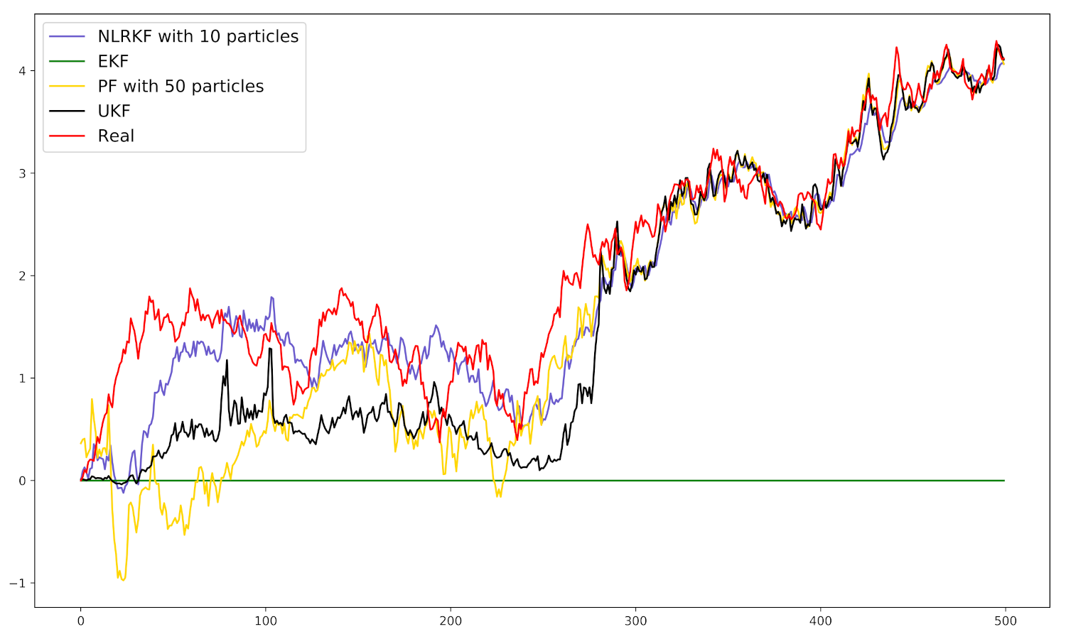
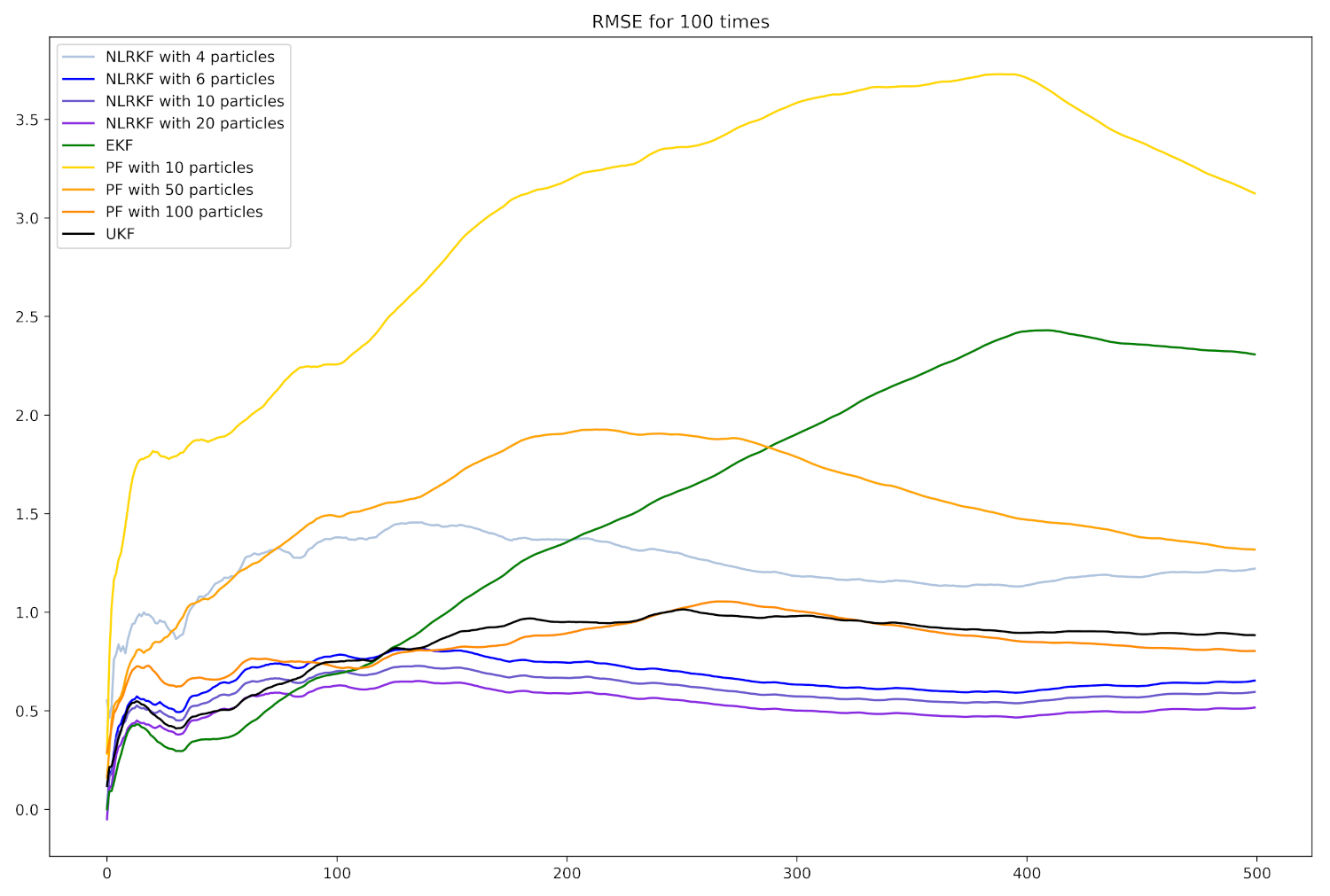
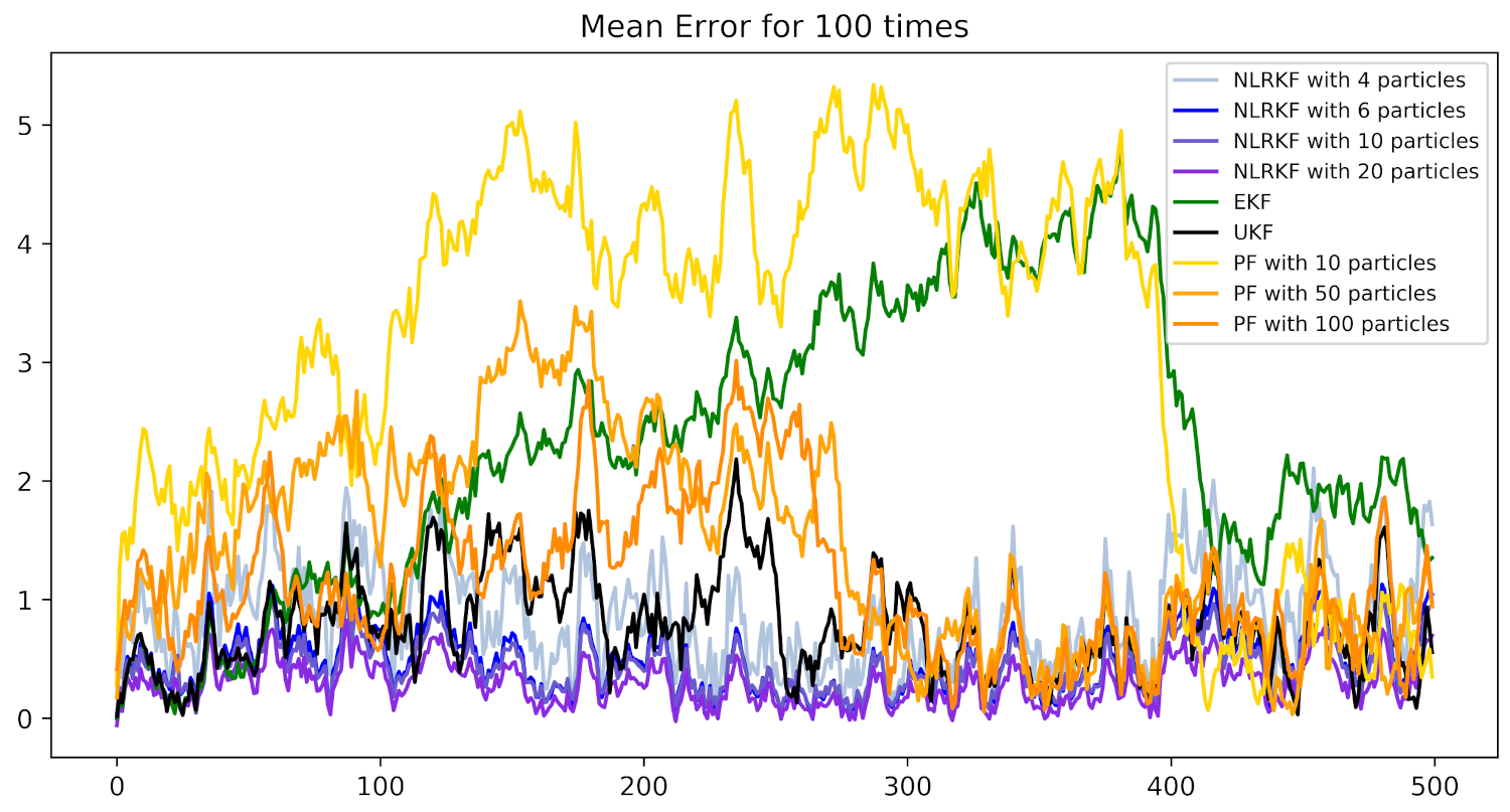
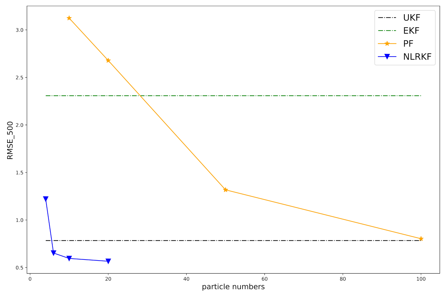
4. Experiments

4.1. Settings

We run our simulations on CPU clusters with Intel Core i9-9880H(2.3CGz/L3 16M) equipped with 16 GB memory.

The total time step is K. We run the simulations for 100 times and assume that the ${\widehat{x}}_k^i$ is the estimation result of real state $x_k^i$ at time step k in the i-th experiment. In order to measure the performances of the numerical algorithms over time, we define the Root Mean Square Error (RMSE) and the mean error at time step k as follows:

$$\begin{array}{cc}\hfill {\mathrm{RMSE}}_k:=& {\displaystyle \frac{1}{100}}\sum _{i=1}^{100}\sqrt{{\displaystyle \frac{1}{k+1}}{\sum }_{j=0}^k{\left({\widehat{x}}_j^i-x_j^i\right)}^2},\hfill \\ \hfill \mathrm{Mean}{\mathrm{Error}}_k:=& \frac{1}{100}\sum _{i=1}^{100}\left|x_k^i-{\widehat{x}}_k^i\right|.\hfill \end{array}$$

(35)

$\mathrm{Mean}{\mathrm{Error}}_k$ is the average estimation error at time k while ${\mathrm{RMSE}}_k$ is the accumulated average estimation error till to time k.

4.2. Numerical Example

We consider the classic cubic sensor here and the model is as follows:

$$\begin{array}{cc}\hfill x_k& =x_{k-1}+w_k,\hfill \end{array}$$

(36)

$$\begin{array}{cc}\hfill y_k& =x_k^3+v_k,\hfill \end{array}$$

(37)

where $x_k\in \mathbb{R}$, $y_k\in \mathbb{R}$, $w_k\sim \mathcal{N}(0,0.01)$, $v_k\sim \mathcal{N}(0,0.01)$, and $k=1,2,\cdots ,K$ with $K=500$. The continuous and continuous-discrete cubic sensor problems have been investigated in [5,11,12], and it has been proved that there cannot exist a recursive finite-dimensional filter driven by the observations for continuous cubic sensor system [23].

We compare our NLRKF with classical EKF, UKF, and PF. We first use 10 symmetric points (or particles) for our NLRKF and 50 particles for PF. The performance in one experiment is shown in Figure 2. Apparently, EKF totally fails to track the real state and other algorithms can track the real state well with different accuracies.

Figure 2. Estimation results in one experiment. The horizontal axis is time step k and the vertical axis is $x_k$ for real state and ${\widehat{x}}_{k|k}$ for filtering algorithms.

To further explore the performance of different algorithms based on 100 experiments, we plot the evolutions of mean error and RMSE over time in Figure 3 and Figure 4. As can be seen from these two figures, NLRKF with 20 particles performs best, followed by NLRKF with 10 particles and 6 particles. UKF is better than PF.

Figure 3. Mean Errors of different filtering algorithms. The horizontal axis is time step k and the vertical axis is $\mathrm{Mean}{\mathrm{Error}}_k$ defined in (35).

Figure 4. RMSE of different filtering algorithms. The horizontal axis is time step k and the vertical axis is ${\mathrm{RMSE}}_k$ defined in (35).

The total estimation error ${\mathrm{RMSE}}_{500}$ and costing times of different methods based on 100 experiments are listed in Table 1, in which $N_{\mathrm{NLRKF}}$ represents the number of particles or points used in NLRKF and $N_{\mathrm{PF}}$ is the number of particles used in PF. We can know that NLRKFs with $20,10$, and 6 particles are the three best performing algorithms considering both RMSE and costing times. We also display the connection of RMSE and number of particles in Figure 5. UKF and EKF are independent of the number of particles, so the two lines are horizontal. The NLRKF surpasses other methods with just 6 particles.

Table 1. The ${\mathrm{RMSE}}_{500}$ and costing times of different filtering algorithms based on 100 experiments.

Method	${\mathbf{RMSE}}_{500}$	Costing Time (s)
EKF	2.3076	0.0206
UKF	0.7840	0.1390
NLRKF ($N_{\mathrm{NLRKF}}=4$)	1.2212	0.0406
NLRKF ($N_{\mathrm{NLRKF}}=6$)	0.6529	0.0729
NLRKF ($N_{\mathrm{NLRKF}}=10$)	0.5959	0.0879
NLRKF ($N_{\mathrm{NLRKF}}=20$)	0.5663	0.1218
PF ($N_{\mathrm{PF}}=10$)	3.1242	0.1163
PF ($N_{\mathrm{PF}}=50$)	1.3175	0.1892
PF ($N_{\mathrm{PF}}=100$)	0.8034	0.2672

Figure 5. ${\mathrm{RMSE}}_{500}$ of filtering algorithms w.r.t. the number of particles or samples.

5. Conclusions

In this paper, we proposed a new LRKF using K–L divergence and symmetric samples. The numerical simulation results show that our algorithm is accurate and efficient. However, the proposed algorithm requires the explicit model of the filtering system. Besides, this algorithm is under the framework of nonlinear Kalman filter, i.e., we approximate the conditional density by single Gaussian density. The approximation can lead to large errors when the conditional density is highly non-Gaussian. How to remove this framework and deterministically propagate the points are our future works.

References

- Kalman, R.E. A new approach to linear filtering and prediction problem. ASME Trans. J. Basic Eng. Ser. D 1960, 82, 35–45. [Google Scholar] [CrossRef] [Green Version]
- Kalman, R.E.; Bucy, R.S. New results in linear filtering and prediction theory. ASME Trans. J. Basic Eng. Ser. D 1961, 83, 95–108. [Google Scholar] [CrossRef]
- Jazwinski, A.H. Stochastic Processes and Filtering Theory; Academic Press: New York, NY, USA; London, UK, 1970. [Google Scholar]
- Simon, D. Optimal State Estimation: Kalman, H Infinity, and Nonlinear Approaches; John Wiley & Sons: Hoboken, NJ, USA, 2006. [Google Scholar]
- Luo, X.; Chen, X.; Yau, S.S.T. Suboptimal linear estimation for continuous–discrete bilinear systems. Syst. Control Lett. 2018, 119, 92–100. [Google Scholar] [CrossRef]
- Gordon, N.J.; Salmond, D.J.; Smith, A.F.M. Novel Approach to Nonlinear/Non-Gaussian Bayesian State Estimation. Radar Signal Process. IEE Proc. F 1993, 140, 107–113. [Google Scholar] [CrossRef] [Green Version]
- Duncan, T.E. Probability Densities for Diffusion Processes with Applications to Nonlinear Filtering Theory and Detection Theory; Technical Report; Stanford University: Stanford, CA, USA, 1967. [Google Scholar]
- Mortensen, R.E. Optimal Control of Continuous Time Stochastic Systems. Ph.D. Thesis, University of California, Berkley, CA, USA, 1966. [Google Scholar]
- Zakai, M. On the optimal filtering of diffusion process. Z. Wahrsch. Verw. Geb. 1969, 11, 230–243. [Google Scholar] [CrossRef]
- Chen, X.; Shi, J.; Yau, S.S.T. Real-time solution of time-varying yau filtering problems via direct method and gaussian approximation. IEEE Trans. Autom. Control 2019, 64, 1648–1654. [Google Scholar] [CrossRef]
- Luo, X.; Yau, S.S.T. Hermite spectral method to 1-D forward Kolmogorov equation and its application to nonlinear filtering problems. IEEE Trans. Autom. Control 2013, 58, 2495–2507. [Google Scholar] [CrossRef]
- Shi, J.; Chen, X.; Yau, S.S.T. A Novel Real-Time Filtering Method to General Nonlinear Filtering Problem Without Memory. IEEE Access 2021, 9, 119343–119352. [Google Scholar] [CrossRef]
- Yau, S.T.; Yau, S.S.T. Real time solution of the nonlinear filtering problem without memory II. SIAM J. Control Optim. 2008, 47, 163–195. [Google Scholar] [CrossRef]
- Lefebvre, T.; Bruyninckx, H.; De Schutter, J. Kalman filters for non-linear systems: A comparison of performance. Int. J. Control 2004, 77, 639–653. [Google Scholar] [CrossRef]
- Steinbring, J.; Hanebeck, U.D. LRKF revisited: The smart sampling Kalman filter (S2KF). J. Adv. Inf. Fusion 2014, 9, 106–123. [Google Scholar]
- Julier, S.J.; Uhlmann, J.K. Unscented filtering and nonlinear estimation. Proc. IEEE 2004, 92, 401–422. [Google Scholar] [CrossRef] [Green Version]
- Majumdar, J.; Dhakal, P.; Rijal, N.S.; Aryal, A.M.; Mishra, N.K. Article: Implementation of Hybrid Model of Particle Filter and Kalman Filter based Real-Time Tracking for handling Occlusion on Beagleboard-xM. Int. J. Comput. Appl. 2014, 95, 31–37. [Google Scholar]
- Morelande, M.R.; Kreucher, C.M.; Kastella, K. A Bayesian Approach to Multiple Target Detection and Tracking. IEEE Trans. Signal Process. 2007, 55, 1589–1604. [Google Scholar] [CrossRef] [Green Version]
- Steinbring, J.; Pander, M.; Hanebeck, U.D. The smart sampling Kalman filter with symmetric samples. arXiv 2015, arXiv:1506.03254. [Google Scholar]
- Liu, Q.; Wang, D. Stein variational gradient descent: A general purpose bayesian inference algorithm. arXiv 2016, arXiv:1608.04471. [Google Scholar]
- Liu, Q. Stein variational gradient descent as gradient flow. arXiv 2017, arXiv:1704.07520. [Google Scholar]
- Härdle, W.K.; Simar, L. Applied Multivariate Statistical Analysis; Springer: Berlin/Heidelberg, Germany, 2019. [Google Scholar]
- Hazewinkel, M.; Marcus, S.; Sussmann, H.J. Nonexistence of finite-dimensional filters for conditional statistics of the cubic sensor problem. Syst. Control Lett. 1983, 3, 331–340. [Google Scholar] [CrossRef] [Green Version]
Publisher’s Note: MDPI stays neutral with regard to jurisdictional claims in published maps and institutional affiliations. |
© 2021 by the authors. Licensee MDPI, Basel, Switzerland. This article is an open access article distributed under the terms and conditions of the Creative Commons Attribution (CC BY) license (https://creativecommons.org/licenses/by/4.0/).