Abstract
Deep neural networks have shown great potential in various low-level vision tasks, leading to several state-of-the-art image denoising techniques. Training a deep neural network in a supervised fashion usually requires the collection of a great number of examples and the consumption of a significant amount of time. However, the collection of training samples is very difficult for some application scenarios, such as the full-sampled data of magnetic resonance imaging and the data of satellite remote sensing imaging. In this paper, we overcome the problem of a lack of training data by using an unsupervised deep-learning-based method. Specifically, we propose a deep-learning-based method based on the deep image prior (DIP) method, which only requires a noisy image as training data, without any clean data. It infers the natural images with random inputs and the corrupted observation with the help of performing correction via a convolutional network. We improve the original DIP method as follows: Firstly, the original optimization objective function is modified by adding nonlocal regularizers, consisting of a spatial filter and a frequency domain filter, to promote the gradient sparsity of the solution. Secondly, we solve the optimization problem with the alternating direction method of multipliers (ADMM) framework, resulting in two separate optimization problems, including a symmetric U-Net training step and a plug-and-play proximal denoising step. As such, the proposed method exploits the powerful denoising ability of both deep neural networks and nonlocal regularizations. Experiments validate the effectiveness of leveraging a combination of DIP and nonlocal regularizers, and demonstrate the superior performance of the proposed method both quantitatively and visually compared with the original DIP method.
1. Introduction
Image denoising [1] is an image processing task with a long history, and has a wide range of application scenarios because noise contamination is inevitable in any image sensing and transmission process. It aims to recover a clean and clear image from a corrupted observation polluted by the noise of various distributions. Despite decades of development, image denoising remains a challenging task due to the need to preserve fine details while suppressing as much noise as possible.
Plenty of sophisticated denoising algorithms have been proposed to infer the original image content based on signal estimation theory. These methods can be roughly classified into two main categories, i.e., model-based methods [2,3] and learning-based methods [4,5]. Model-based methods generally establish optimization objective functions consisting of an observation model and an image prior model, which can be constructed and solved from a Bayesian perspective, using the maximum a posteriori (MAP) or the minimum mean square error (MMSE) estimators. Published works have designed a large amount of elaborate prior models. At first, researchers believed that images are generally sparse in the gradient domain and transform domain, and proposed the well-known total variation (TV) regularizer [6] and transform domain sparsity [7]; they immediately found that these regularizers could not describe the local features of images well. Hence, patch-based sparse representation models [8] then appeared to express more complex local edges and textures in a patch-wise order. However, they still ignore the relationship among patches. In order to exploit the dependence between image patches, researchers have proposed various types of structural sparsity-based models, ranging from tree-structured wavelet sparsity, block-structured sparsity, and nonlocal sparsity [9,10]. Among them, nonlocal sparse models that explore spatial self-similarity in the image itself have shown the most benefit to image denoising. Buades et al. proposed the non-local means (NLMs) method [11] to perform denoising by averaging similar patches in the image. Dabov et al. then proposed the block-matching and 3D filtering (BM3D) method [12], which takes advantage of both the space and frequency domains. It firstly groups similar 2D image blocks into 3D data arrays, and secondly performs the 3D wavelet transform on the obtained 3D data arrays, thirdly applies the collaborative filtering on the 3D wavelet coefficients for denoising. After that, wiener filtering is utilized to carry out denoising again for the purpose of obtaining the final estimation. Besides these two classic methods, nonlocal image denoising methods also include the low-rank approach [13], which discovers the matrices grouped by 2D image blocks that have the low-rank property; the nonlocal model is based on a weighted nuclear norm constraint and its varieties [14,15], and is an extension of the low-rank approach but assigns different weights to the coefficients; and the Bayesian modeling method, i.e., the simultaneous sparse coding with Gaussian scale mixture (SSC-GSM) method [16].
In contrast to model-based methods that enforce a solution to obey some well-designed prior distributions based on statistics, learning-based methods directly learn mapping functions or sparse transform bases to estimate the missing high-frequency details from the observed noisy image or a large number of external samples. They can be divided into two categories by either learning the sparse representation or learning the deep networks. The well-known K-SVD dictionary learning algorithm [17] belongs to the first category. It trains an offline dictionary on an external large set of image patches or an online dictionary using the noisy patches in the image itself in order to have universally good representation for all test images. The nonlocally centralized sparse representation (NCSR) [18] and external patch prior guided internal clustering (EPPGIC) [19] methods have extended dictionary learning to nonlocal domains via the group sparse coding and Gaussian mixture models learning, respectively. Trainable nonlinear reaction diffusion (TNRD) [20], which tries to turn nonlinear diffusion models into a learnable deep neural network, denoising CNN (DnCNN) [21], that introduces the idea of residual learning, and a memory network (MemNet) [22], which designs memory blocks, can be classified into the second category. In addition, to obtain the true noise level, the noise estimation subnetwork is used in a convolutional blind denoising network (CBDnet) [23]. Recently, a popular attention mechanism has been introduced in an attention-guided network (Adnet) [24] for more accurate denoising. In order to extend the deep neural networks to solve more common image restoration problems and obtain better flexibility, combining the optimization-based methods and deep-learning-based image denoising methods has also been proposed [25,26]. Image restoration with deep CNN denoiser prior (IRCNN) [26] has been designed to integrate a set of pre-trained deep neural networks into the half-quadratic splitting framework for various types of image restoration tasks, including image denoising. Denoising a prior-driven deep neural network [27] also plugs the CNN denoiser into the half-quadratic splitting method as an image prior, which is similar to IRCNN but more adaptive, as both the CNN denoisers and the back-projection modules can be jointly optimized. Besides, an autoencoder denoiser is plugged into the objective function of image restoration in [28]. The resulting autoencoder error is then backpropagated using gradient descent.
Despite great achievements, the above deep-learning-based methods rely heavily on a large number of clean samples and a significant amount of training time. To address this issue, unsupervised deep-learning-based methods [29,30] can achieve precise recovery without clean data. While Stein’s unbiased risk estimate (SURE) is used to train a deep neural network in an unsupervised fashion in [29], generative adversarial networks (GANs) trained with noisy images are adopted to yield noise-free images in [30]. Nevertheless, they still require training samples, even for noisy images. Noise2Noise [31] and deep image prior (DIP) [32] are the two most representative algorithms that only demand a small amount of training samples. In contrast to the Noise2Noise method, which demands two independent observations of the corrupted scene, the DIP method only requires the current noisy image and thus behaves more intelligently. In order to improve the performance of DIP, researchers have proposed to modify its objective function by either using SURE [33] or adding the TV sparse term [34] for more stable reconstruction. In addition, integrating DIP into optimization-based methods, such as the alternating direction method of multipliers (ADMM) framework, has been proven to be an effective mean of improvement in [35,36]. While the TV sparse term is utilized by ADMM-DIPTV [35], leading to an l2 norm proximity operator being necessary to complete a step of ADMM, the regularization by denoising (RED) technique that turns an existing denoiser into a regularizer has been merged with DIP by DeepRED in [36]. In general, the performance of unsupervised deep-learning-based methods is worse than that of supervised methods.
In this paper, we focus on enhancing the performance of an unsupervised deep-learning-based method, i.e., the DIP method. The contributions can be summarized as follows: (1) we utilize the technique of the plug-and-play prior to explore the power of existing denoisers, i.e., NLM and BM3D for regularizing the solution of DIP; (2) we propose a novel objective function that is a linear combination of a data fitting term that enforces the output of DIP to be close to the observations and a prior term corresponding to two nonlocal sparsity-based methods, i.e., NLM and BM3D; (3) we adopt the ADMM method to separate the original complex problem into two simple subproblems via the variable splitting technique for solving the proposed objective function. Then, we can independently solve the network training problem based on the DIP process and image restoration problem via a proximal denoising operation. Thanks to the process of iterative optimization and nonlocal regularization, our method has better adaptability and flexibility, and thus gains better performance than the original DIP method.
2. Background
2.1. Image Denoising Problem and Iterative Method
The image restoration includes denoising attempts to restore images that have been degraded in sensing and transmission processes. It is a common preprocessing task in computer vision, which directly affects the accuracy of subsequent analysis. Mathematically, the image restoration can be considered as a linear inverse problem:
where is the image to be restored, is a degradation matrix, is the measurement of , and corresponds to the measurement noise, which is usually assumed to be additive white Gaussian (AWGN) of variance . For the problem of image denoising, is an identity matrix. Given the degraded measurement, , one can recover by least-squares estimation:
Considering that practical inverse problems are often ill-posed or seriously deteriorated, the regularized least-squares estimation is more favorable:
where is the sparse regularization term based on some prior knowledge. The regularization parameter pays a role of balancing the trade-off between data fidelity and prior constraining.
By deriving with respect to and making the derivative equal to 0, we have the solution of Equation (2), i.e., , or we can solve Equation (2) with gradient-descent-based methods. is the transpose of . As for Equation (3), it will take an extra step, i.e., a proximal denoising step when using gradient-descent-based methods, e.g., an iterative shrinkage–thresholding (IST) method, a fast iterative shrinkage–thresholding algorithm (FISTA), and Nesterov’s algorithm (NESTA) [37]. The alternating expressions in the IST algorithm, also known as the proximal gradient method, are:
where is the estimate of at iteration k, and is the result of the gradient optimization of . is a smooth convex function with a Lipschitz constant, . Equation (4) is the gradient search step wherein denotes the gradient of the function, , at the point , and the step size is . Equation (5) is the the proximal mapping associated with function , which is defined as . We consider the simplest case, i.e., , where denotes the wavelet transform of . Then, the proximal mapping is equal to perfroming the wavelet denoising on with a threshold of .
2.2. Deep Image Prior
The supervised deep-learning-based methods attempt to solve the image restoration problem by making use of deep neural networks that learn the mapping from degraded images to clean counterparts with a set of example pairs. The learning of deep networks is accomplished by back-propagating the error between degraded images and target images, which can be defined by a mean square error (MSE) base loss function:
where and denote the i-th pair of degraded and original image patches in a large image set with the total number of G, respectively, and denotes the reconstructed image patch by the network with parameter set . We can solve Equation (6) by means of standard stochastic optimization algorithms, e.g., stochastic gradient descent (SGD) or adaptive moment estimation (ADAM) [38]. Once the network training is finished, the optimal solution for a given degraded image is . The success of the supervised deep-learning-based methods relies deeply on the large training set, whose total number could be tens of thousands.
In some practical sensing applications, it is hard to collect a large training set, for example, in the field of medical imaging and remote sensing; therefore, we focus on unsupervised deep-learning-based methods. The deep image prior (DIP) method introduced by Ulyanov et al. in [10] has been shown to be most favorable due to the fact that it only requires the noisy observation itself without any training samples. It solves the following minimization problem:
and presents as the recovered image. It is pleasantly surprised to be found that with the help of convolutional neural network (CNN) architecture, one can approximate the clean image by using a fixed random vector, , and the degraded image, . Thus, the deep network can be regarded as an implicit image prior, exploiting the image self-similarity to suppress noise. Since the DIP method does not have the training samples, it corresponds to an online learning method which solves Equation (7) with the ADAM method.
3. Nonlocal Regularized Deep Image Prior for Image Denoising
3.1. The Proposed Model
Although DIP has been demonstrated to be quite effective for image denoising, its results still fall short when compared to supervised deep-learning-based methods that have been shown to be state of the art. In order to improve the performance of DIP, we propose to boost it using an extra prior to perform regularization. Since the performance of nonlocal sparsity-based methods has been shown to be close to that of DIP, the explicit prior chosen by us is a nonlocal constraint that attempts to jointly explore the power of dual filtering in the spatial and frequency domains by combining nonlocal means and the BM3D denoising scheme. Mathematically, we try to solve the following constrained minimization problem:
where:
In Equation (9), and denote the prior constraint corresponding to nonlocal means [11] and the BM3D denoising [12] scheme, respectively. and are two regularization parameters. Through the use of the plug-and-play prior, we do need to offer explicit expression of and , and can take them as black boxes which takes the noisy observation as an input, and the denoised image as an output. From Equation (8) and Equation (9), we can see that the combination of complementary regularizers is exploited in our restoration model, including a deep-neural-network-based prior, i.e., DIP and a nonlocal dual-filtering-based prior.
3.2. Plug-and-Play ADMM Method
The proposed model, i.e., Equations (8) and (9) cannot be solved by directly applying the DIP method, which involves computing the derivative of denoisers during the process of back-propagation. For most of the denoisers, the denoising operators do not have an explicit input–output relation, thus it is not easy to compute their derivatives. To remedy this problem, we resort to the alternating direction method of multipliers (ADMM) method [39], which is a famous variable splitting technique, and is able to separate in the nonlocal prior term from the constraint of our minimization problem, i.e., . With the help of the augmented Lagrangian (AL), we can turn the constraint into a penalty term, and then merge it into the objective function as follows:
where is the penalty parameter that is a positive scalar, and the vector is the Lagrangian multipliers associated with the constraint . Merging the last two terms, we have the scaled form of the AL:
Using the method of alternating optimization, we can simultaneously learn the parameters of deep neural network, , and then recover the image. Firstly, we estimate the parameters set, , for fixed and , after which we have:
This loss function is very close in spirit to the one solved in the original DIP method. It is added with the second l2 norm term when compared to the one in the original DIP method; however, it still can be solved by means of back-propagation via applying a gradient-based method, e.g., ADAM. In particular, while the output of the network, , is forced to be close to the noise observation, , in the original DIP method, our modified method makes it possible to approximate both and the intermediate result, . Hence, the loss error to be back-propagated is a linear combination of the l2 distance between and , and the one between and .
Secondly, given the parameters set, , and , we need to recover the image, . At this point, Equation (11) becomes:
This is exactly the proximal denoising operation. By substituting with Equation (9) we have:
Note that the regularization parameter, , has been merged into and . The resulting composite sparse problem can easily be solved by the method of a composite splitting algorithm (CSA) [40] based on the technique of variable splitting and operator splitting. The CSA decomposes the difficult composite regularization problem, i.e., Equation (14) into two simpler constraint subproblems, and then solves each of them separately. According to the process of the CSA, we first get the following subproblems:
Secondly, the solution of Equation (14) is obtained by a linear combination of and with the weights and as follows:
Finally, for fixed and , the multiplier vector is computed by:
The solutions of Equations (15) and (16), and , correspond to the denoised results of NLM and BM3D denoising, respectively. For NLM, given a collection of similar patches, a nonlocal mean filter is adopted to estimate the means of these patches, as follows:
where denotes the i-th image patch, and the weight is computed by:
In Equation (20), denotes the exemplar patch and is the parameter representing the variance. in our experiments. For BM3D denoising, we only consider the initial hard thresholding step of the BM3D method, which is offered as follows:
as we have observed that the secondary Wiener filtering step is of little use in our scheme. In Equation (21), and denote the 3D data arrays and the 3D wavelet transform. Hence, the l0 norm in Equation (21) means that the 3D wavelet coefficients should be sparse. It leads to a hard thresholding step. In practice, the regularization parameters and , which have been proven to be closely connected with the thresholds of denoising, do not need to be set. Instead of setting and , we turn to determine their thresholds. While the NLM method does not have a threshold, the threshold of BM3D denoising is determined by the variance of noise, , which can be obtained by maximum likelihood estimation:
In general, the proposed algorithm is summarized in Algorithm 1, named “Nonlocal Regularized Deep Image Prior (NR-DIP)”. Exploring the power of complementary priors and ADMM iterations is implemented in our method for image denoising. The flow chart and the symmetric CNN architecture of our method is represented in Figure 1, from which it can be seen that our network architecture is consistent with the one in [32], which is based on the classical U-Net structure, adopting the model of encoder–decoder. While the “Convolution + Down Sample + Batch Normalization + Leaky ReLU + Convolution + Batch Normalization + Leaky ReLU” blocks are carried out for feature extraction in the encoder units, the “Batch Normalization + Convolution + Batch Normalization + Leaky ReLU + Convolution + Batch Normalization + Leaky ReLU + Up Sample” blocks are performed for image restoration in the decoder units. Skip connections are added for capturing image structures of different characteristic scales. The parameters of the network are listed in Table 1. From Figure 1 and the pseudo code of the proposed algorithm, we can see that our method is based on the ADMM method. In each ADMM iteration, we firstly perform the network learning via the ADAM method to obtain the network parameters, , and we then estimate the noise standard deviation, . Finally, we recover the image, , by using the network output, , and the multiplier, , of the previous iteration and then update the multiplier.
| Algorithm 1. Nonlocal Regularized Deep Image Prior. |
| Input:y, K, , , , , . |
Fork = 0 to K − 1 do
|
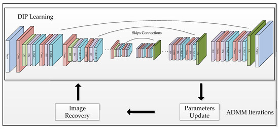
Figure 1.
The flow chart and the CNN architecture based on the U-Net used in our method.

Table 1.
The parameters of the network.
4. Experiments
In order to verify the excellent performance of the proposed NR-DIP for image denoising, we compare our method with nine image restoration algorithms, including two nonlocal sparsity-based methods, i.e., NLM [11] and CBM3D [12] (“C” denotes color image), two supervised deep-learning-based methods, i.e., FFDNet [41] and IRCNN [26], which have been shown to be superior to the well-known benchmark method, i.e., DnCNN [21], and an unsupervised deep-learning-based method, i.e., DIP [32]. Among these comparison methods, NLM, CBM3D, and DIP are three methods that are the foundation of our method. Through the comparisons between NLM, CBM3D, DIP, and NR-DIP, one can validate the benefit of complementary priors. CBM3D can be considered as the most efficient nonlocal sparsity-based method. While FFDNet represents a class of deep-learning-based methods which train direct mapping from degraded images to clean images, IRCNN represents the ones that merge deep neural networks into optimization-based methods. In fact, we also considered including the ADMM-DIPTV [35] method into our comparisons, but we found that it suffers from severe performance degradation in the later stage of iteration. Both ADMM-DIPTV and our method are based on ADMM and DIP; however, ADMM-DIPTV only combines the TV constraint into the framework of DIP due to its convexity. Introducing the use of the plug-and-play prior scheme makes the adoption of existing powerful denoising algorithms available and flexible, greatly extending the recovery ability of DIP.
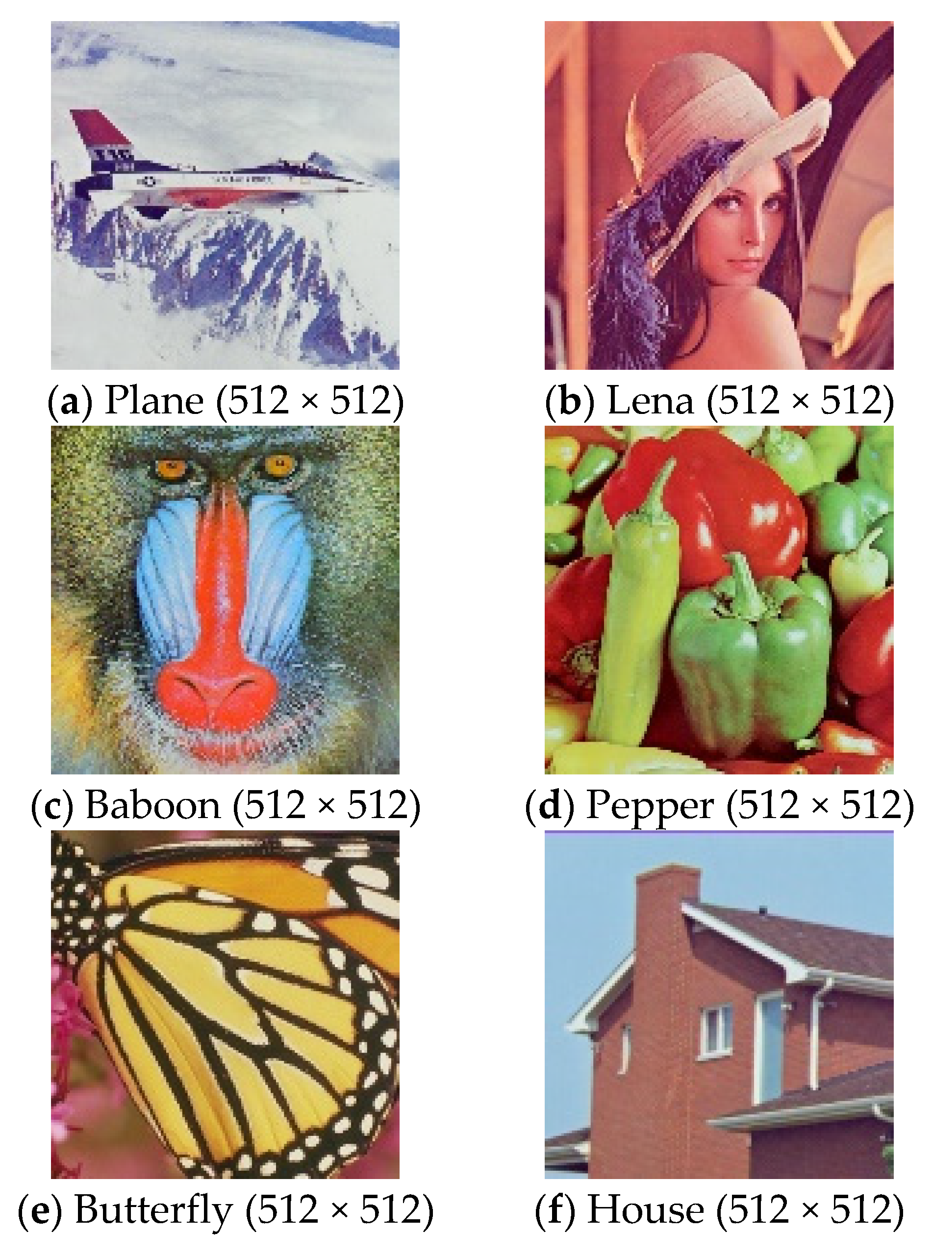
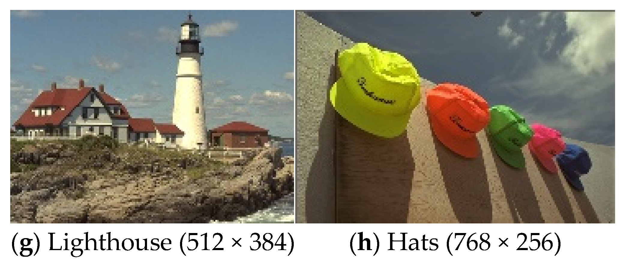
Figure 2 provides eight test natural images used in our experiments with various sizes. We generated noisy measurements by adding varying amounts of additive white Gaussian noise to the test images. The range of the standard deviation of Gaussian noise includes 25, 30, 35, 40, 50, 60, and 75. Then, we applied the comparison methods to execute denoising. The peak signal-to-noise ratio (PSNR) and structural similarity (SSIM) [42,43], shown in Equation (23) and Equation (24):
are used to quantitatively evaluate the qualities of the reconstruction results. In Equation (23), m and n denote the image size. In Equation (24), , , , , and are the average intensities, standard deviations, and cross-covariance of a clean image, y, and an evaluated image, x, respectively. For fair comparisons, we have downloaded codes from the websites of the authors, adopting the default experiment settings. The main parameters of the proposed NR-DIP algorithm include: (1) the weights of the linear combination, i.e., and in Equation (16); (2) the parameter of ADMM, , in Equation (14); and (3) the learning rate of training is set to 0.008. Due to the long running time of BM3D, we apply it once every 100 iterations of the ADMM to save time. The DIP-based methods were implemented in the Python language with a PyTorch framework and run on an NVIDIA GTX 3090 GPU. NLM and CBM3D were implemented in the Python language, but were run without a GPU. FFDNet and IRCNN were implemented in the MATLAB language and also run without GPU because they are already fast. The experimental results including objective quality, subjective quality, and runtime are present.


Figure 2.
Test images used for image denoising experiments.
We first present the experimental results in terms of objective quality. While the PSNR results of the comparison methods on the set of test images shown in Figure 2 are offered in Table 2, the corresponding SSIM results are provided in Table 3. Since FFDNet and IRCNN do not provide the learned models with a noise standard deviation of 60 and 75, we have not given their corresponding comparison results. It can be seen in these tables that the supervised deep-learning-based methods, i.e., FFDNet and IRCNN, outperform others regardless of a high or low noise level. In both of them, the FFDNet algorithm performs slightly better. Apart from them, the proposed NR-DIP method has achieved highly competitive denoising performance compared to other leading algorithms, consisting of the unsupervised deep-learning-based methods, i.e., DIP and the nonlocal sparsity-based methods, i.e., NLM and CBM3D. The proposed NR-DIP method outperforms the original DIP by up to 0.5 dB on average, which has verified the effectiveness of our modifications. By employing NLM and BM3D to regularize the solution of DIP, the NR-DIP method can combine the power of nonlocal denoising and deep-learning-based denoising. It leads to a better solution, which is enforced by complementary priors and is optimized with the ADMM method when compared to the original DIP. Among the nonlocal sparsity-based methods, the CBM3D method is obviously better than the NLM. On average, NR-DIP falls behind FFDNet by less than 1.1 dB. (1) Compared to the supervised deep-learning-based methods FFDNet and IRCNN, our method is generally worse. It is reasonable that FFDNet and IRCNN require thousands of samples to train the network, acquiring a good generalization ability; however, our method solely puts the noisy observation into the network without requiring any clean images, and thus is prone to over-fitting. Nevertheless, our method is quite useful for some applications in the case of a lack of sample data. (2) Compared to the nonlocal sparsity-based methods NLM and CBM3D, our method usually performs better due to the joint use of NLM, CBM3D, and DIP. (3) Compared to the original DIP method, our method usually performs better. This is not only because of combining the power of nonlocal denoising and deep-learning-based denoising, but also because it benefits from the ADMM iteration that leads to a better solution by alternating optimization. However, using NLM and CBM3D sometimes slightly reduces the performance of the DIP method for the image with a complex texture, e.g., the Baboon image, and the lower-power noise environment. While the output of the network, , is forced to be close to the noise observation, , in the original DIP method, our modified method makes it approximate both and the intermediate result, . Therefore, when and contain similar information, our algorithm does not improve by much. With regard to SSIM, as shown in Table 3, the results of the original DIP are worse than that of CBM3D, which is inconsistent with the PSNR results. However, our method does not follow the original DIP to get worse in terms of SSIM. It is demonstrated that the nonlocal regularized scheme helps to maintain structural information while removing noise.
Table 2.
The PSNR (dB) results of different methods with varying amounts of additive white Gaussian noise.
Table 3.
The SSIM results of different methods with varying amounts of additive white Gaussian noise.
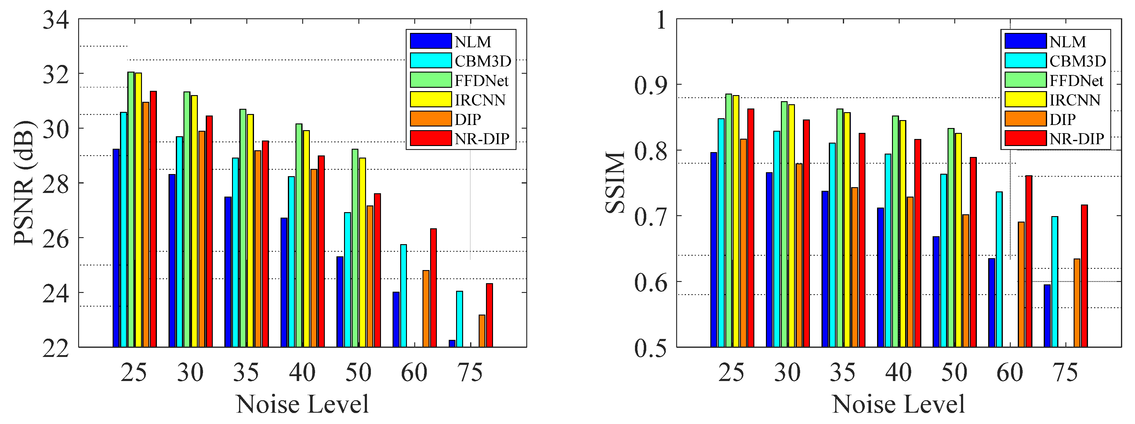
In order to show the comparison results more vividly, Figure 3 provides the average PSNR and SSIM values of the comparisons between the reconstructions by different methods. The order of performance in terms of PSNR from good to bad is FFDNet, IRCNN, NR-DIP, DIP, CBM3D, and NLM, while the in terms of SSIM it is FFDNet, IRCNN, NR-DIP, CBM3D, DIP, and NLM. The average PSNR results of NLM, CBM3D, FFDNet, IRCNN, DIP, NR-DIP are 27.4 dB, 28.9 dB, 30.7 dB, 30.5 dB, 29.1 dB, and 29.6 dB for the noise standard deviation ranging from 25 to 50, respectively, while the average PSNR results of NLM, CBM3D, DIP, and NR-DIP are 23.1 dB, 24.9 dB, 24.0 dB, and 25.3 dB for the noise standard deviation of 60 and 75, respectively. For a higher noise level, the difference between algorithms increases, but the order remains unchanged. Note that the NR-DIP method is better than the original DIP, NLM, and CBM3D methods, and has verified the effectiveness of the proposed combination scheme. Although the results of NR-DIP still fall short when compared to the supervised state-of-the-art methods, NR-DIP has been shown to be quite effective, and demonstrated successfully the problem of image denoising.
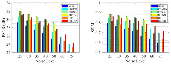
Figure 3.
The average PSNR (dB) and SSIM results of competing methods with different noise levels.
4.1. Subjective Quality Evaluation
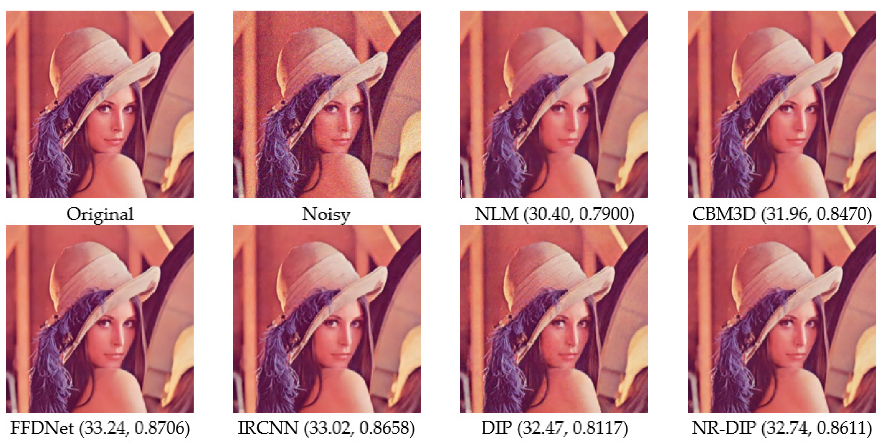
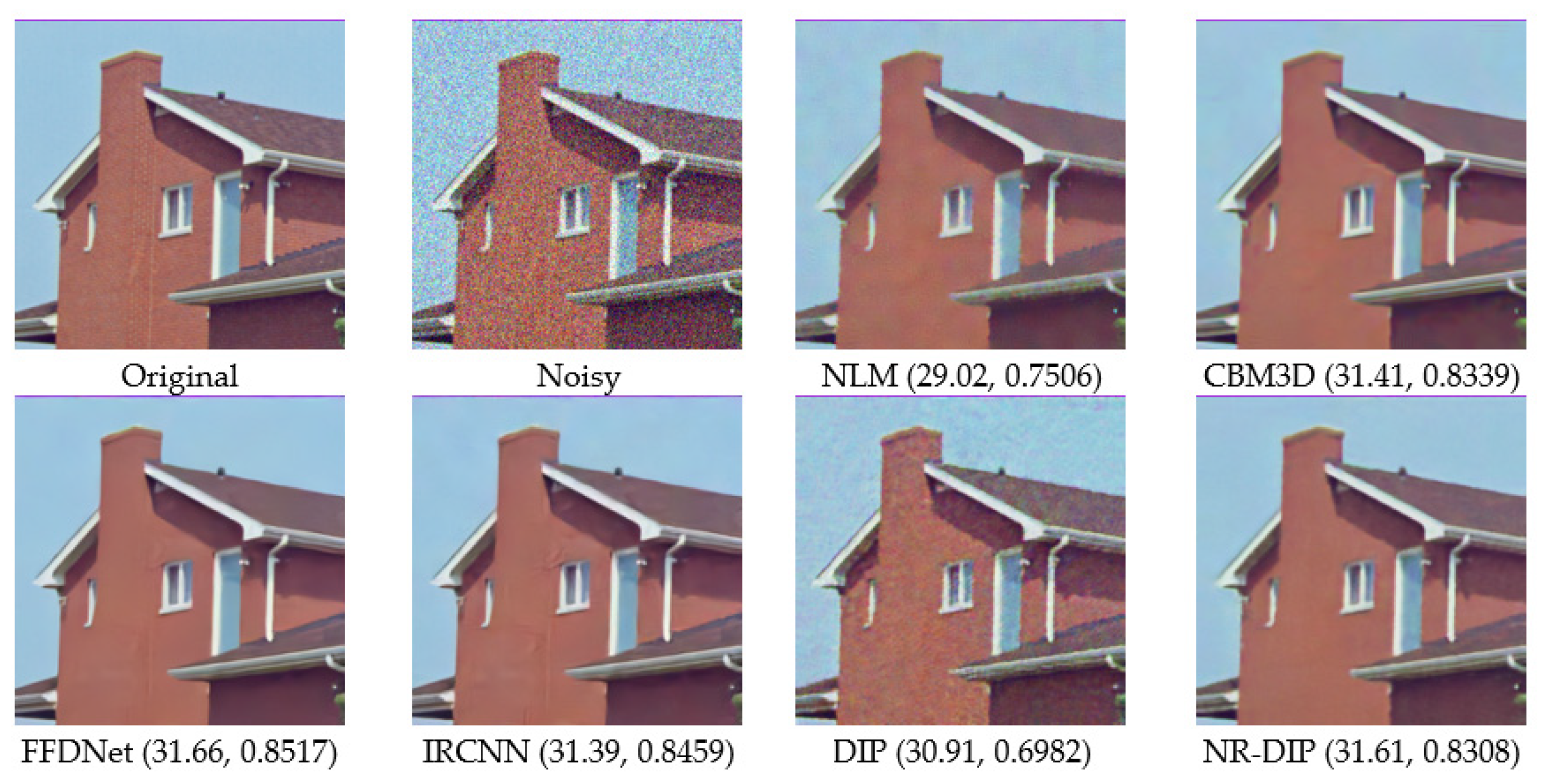
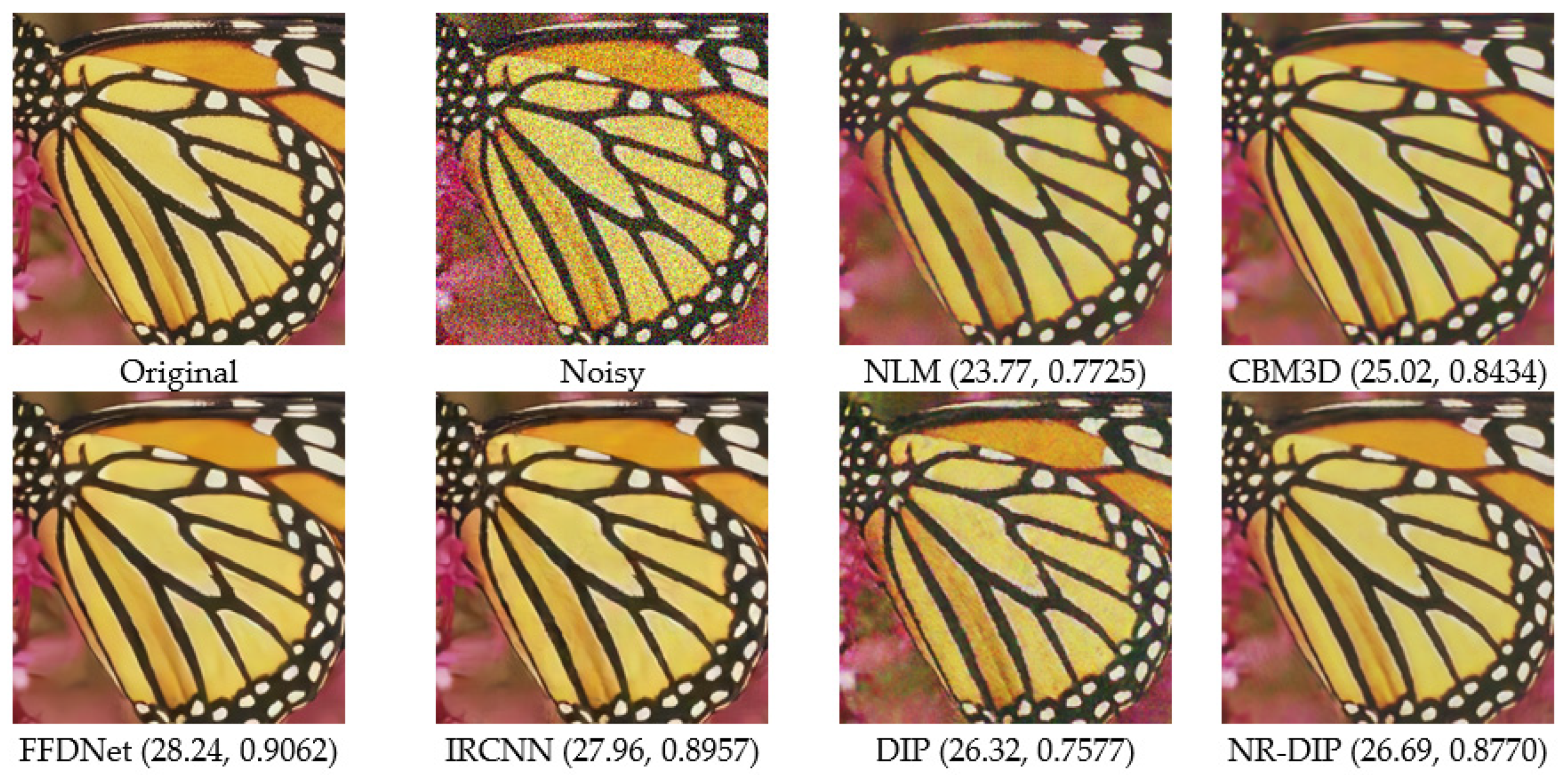
Visual comparisons between the restoration results by competing methods are provided in Figure 4, Figure 5, Figure 6, and Figure 7 with the standard deviation of noise, i.e., sigma = 25, 35, 50, and 75 representing the performance under various kinds of noise environments. From these figures, one can clearly see that the best denoising results are still achieved by a supervised deep-learning-based method, i.e., FFDNet. Meanwhile, IRCNN performs comparably with FFDNet, following closely. For the rest of the algorithms that do not rely on large amounts of training data, the proposed algorithm NR-DIP performs better than others, and enjoys great advantages in producing clearer images, e.g., the edges and fine textures. While the NLM method over-smoothed and provided a lack of image details, meaning that its denoising ability is relatively poor, the CBM3D method results in ringing artifacts due to the truncation operation in the frequency domain. In contrast, the restoration results by DIP suffers from noticeable artifacts, especially for a higher noise level when compared to the one by NR-DIP, which delivers excellent image contrast and clear details due to its capability of achieving a better spatial adaptation by using complementary priors. For a higher noise level, the denoised images of all competing algorithms are seriously degraded, but the proposed NR-DIP method still shows its advantages in recovering more a detailed image when compared to the competing ones, except for FFDNet and IRCNN. These results verify again that the combination of CBM3D, NLM, and DIP is reasonable.
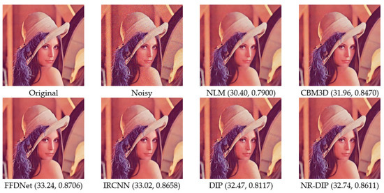
Figure 4.
Visual comparisons of the Lena image with Gaussian noise with a standard deviation of 25 (PSNR and SSIM values in brackets).
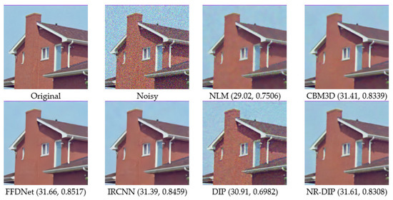
Figure 5.
Visual comparisons of the House image with Gaussian noise with a standard deviation of 35 (PSNR and SSIM values in brackets).
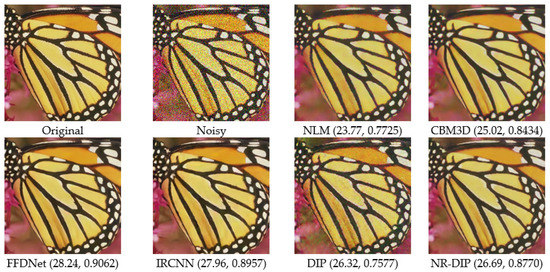
Figure 6.
Visual comparisons of the Butterfly image with Gaussian noise with a standard deviation of 50 (PSNR and SSIM values in brackets).
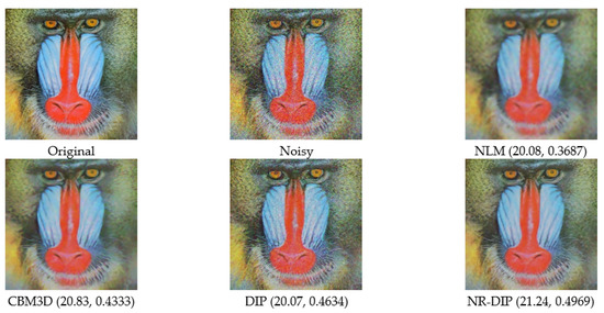
Figure 7.
Visual comparisons of the Baboon image with Gaussian noise with a standard deviation of 75 (PSNR and SSIM values in brackets).
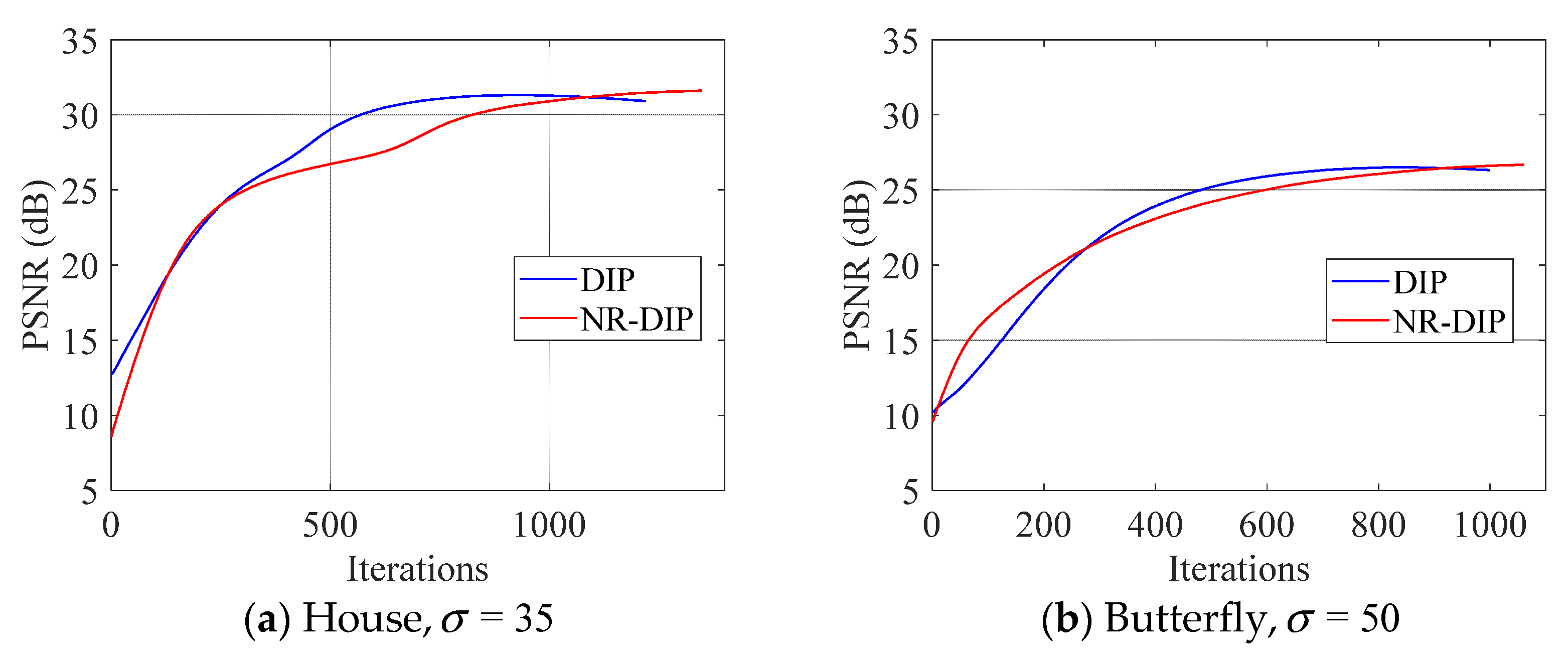
4.2. Runtime Comparison
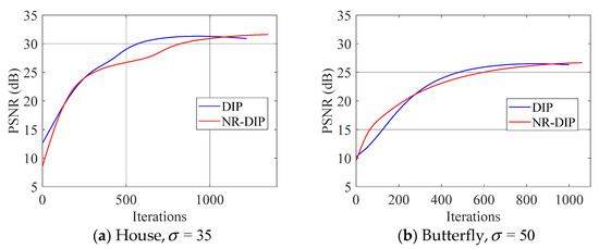
In order to evaluate the running time and convergence of the proposed method, we also traced the runtime and PSNR of each iteration for the original DIP method as well as our method. The results are illustrated in Figure 8, which presents the iteration number vs. PSNR curves of the House and Butterfly images, respectively. In particular, the performance curves in Figure 8 correspond to the experiment in Figure 5 and Figure 6. In Figure 8, the NR-DIP method achieves the better performance in terms of PSNR and iterations than the original DIP after around 1000 iterations. These curves validate that the proposed method NR-DIP can converge to a good denoised result in a reasonable number of iterations.
The average runtime to recover an image with a size of 512 × 512 by FFDNet, IRCNN, NLM, CBM3D, DIP and NR-DIP, are about 1.23 s, 2.26 s, 2.68 s, 24.80 s, 148.09 s and 244.16 s, respectively. We list the average runtime in Table 4. The supervised deep learning methods, FFDNet and IRCNN, are fast and take only several seconds to remove noise for an image, but they take a lot of time to train deep neural networks. The unsupervised deep learning methods use an online learning scheme, resulting in a slow speed. Merging nonlocal regularization into the framework of DIP in our method definitely increases the running time, but within a reasonable range.
Table 4.
The average runtime of different denoising methods.
5. Conclusions
We have proposed an effective iterative algorithm equipped with the deep image prior and the plug-and-play nonlocal priors for image denoising. Our work contributes the following: First, guided by information theory, the use of complementary constraints was introduced to construct the nonlocal regularized deep image prior model for an unsupervised deep-learning-based image denoising problem. It can substantially enhance the performance of the original DIP by jointly utilizing the nonlocal information in the spatial and frequency domains. Second, an effective ADMM-based algorithm with excellent denoising ability is proposed in this paper to make the proposed model much easier to be solved by using the technique of variable splitting. Finally, our experiments on several natural images demonstrate the superiority of the proposed algorithm to two nonlocal sparsity-based denoising algorithms and the original DIP method. While this work has designed a flexible combination of the unsupervised deep-learning-based method DIP and the plug-and-play priors in the framework of ADMM, in addition to demonstrating promising performance, we plan to combine the DIP with other supervised deep-learning-based methods to boost denoising performance in future work.
Author Contributions
Conceptualization, L.L. and Z.X.; Funding Acquisition, Z.X.; Investigation, L.L.; Project Administration, L.L.; Software, Z.X.; Supervision, Z.L.; Validation, J.H.; Writing—Original Draft, Z.X.; Writing—Review and Editing, L.L. All authors have read and agreed to the published version of the manuscript.
Funding
This work was supported by the National Natural Science Foundation of China (62001184), the Guangdong Basic and Applied Basic Research Foundation (2019A1515111087), the Science and Technology Planning Project of Huizhou (2020SD0403031), the Project of Young Innovative Talents from Educational Commission of Guangdong Province (2018KQNCX247), and the Doctoral Scientific Research Foundation of Huizhou University (2018JB024, 2018JB025).
Data Availability Statement
Not applicable.
Acknowledgments
We gratefully acknowledge the helpful comments and suggestions of the reviewers, which have improved the presentation. This work was also supported by the Program for Innovative Research Team of Huizhou University (IRTHZU).
Conflicts of Interest
The authors declare no conflict of interest.
References
- Yin, Z.; Xia, K.; He, Z.; Zhang, J.; Wang, S.; Zu, B. Unpaired Image Denoising via Wasserstein GAN in Low-Dose CT Image with Multi-Perceptual Loss and Fidelity Loss. Symmetry 2021, 13, 126. [Google Scholar] [CrossRef]
- Beck, A.; Teboulle, M. Fast gradient-based algorithms for constrained total variation image denoising and deblurring problems. IEEE Trans. Image Process. 2009, 18, 2419–2434. [Google Scholar] [CrossRef] [Green Version]
- Zha, Z.; Yuan, X.; Wen, B.; Zhou, J.; Zhu, C. Group Sparsity Residual Constraint with Non-Local Priors for Image Restoration. IEEE Trans. Image Process. 2020, 29, 8960–8975. [Google Scholar] [CrossRef] [PubMed]
- Chen, S.; Xu, S.; Chen, X.; Li, F. Image Denoising Using a Novel Deep Generative Network with Multiple Target Images and Adaptive Termination Condition. Appl. Sci. 2021, 11, 4803. [Google Scholar] [CrossRef]
- Xie, Z.; Liu, L.; Yang, C. An Entropy-Based Algorithm with Nonlocal Residual Learning for Image Compressive Sensing Recovery. Entropy 2019, 21, 900. [Google Scholar] [CrossRef] [Green Version]
- Vese, L.A.; Osher, S.J. Image Denoising and Decomposition with Total Variation Minimization and Oscillatory Functions. J. Math. Imaging Vis. 2004, 20, 7–18. [Google Scholar] [CrossRef] [Green Version]
- Hou, Z. Adaptive singular value decomposition in wavelet domain for image denoising. Pattern Recognit. 2003, 36, 1747–1763. [Google Scholar] [CrossRef]
- Gong, W.; Li, H.; Zhao, D. An Improved Denoising Model Based on the Analysis K-SVD Algorithm. Circuits Syst. Signal Process. 2017, 36, 4006–4021. [Google Scholar] [CrossRef]
- Zha, Z.; Zhang, X.; Wang, Q.; Bai, Y.; Tang, L. Image denoising using group sparsity residual and external nonlocal self-similarity prior. Neurocomputing 2018, 275, 2294–2306. [Google Scholar] [CrossRef] [Green Version]
- Li, L.; Xiao, S.; Zhao, Y. Image Compressive Sensing via Hybrid Nonlocal Sparsity Regularization. Sensors 2020, 20, 5666. [Google Scholar] [CrossRef]
- Buades, A.; Coll, B.; Morel, J.M. Image denoising by non-local averaging. In Proceedings of the IEEE International Conference on Acoustics, Speech, and Signal Processing (ICASSP), Philadelphia, PA, USA, 23 March 2005; pp. 25–28. [Google Scholar]
- Dabov, K.; Foi, A.; Katkovnik, V.; Egiazarian, K. Image denoising by sparse 3-d transform-domain collaborative filtering. IEEE Trans. Image Process. 2007, 16, 2080–2095. [Google Scholar] [CrossRef]
- Dong, W.; Shi, G.; Li, X. Nonlocal Image Restoration with Bilateral Variance Estimation: A Low-Rank Approach. IEEE Trans. Image Process. 2013, 22, 700–711. [Google Scholar] [CrossRef]
- Gu, S.; Zhang, L.; Zuo, W.; Feng, X. Weighted Nuclear Norm Minimization with Application to Image Denoising. In Proceedings of the IEEE Conference on Computer Vision and Pattern Recognition (CVPR), Columbus, OH, USA, 23–28 June 2014; pp. 2862–2869. [Google Scholar]
- Deng, H.; Tao, J.; Song, X.; Zhang, C. Estimation of the parameters of a weighted nuclear norm model and its application in image denoising. Inf. Sci. 2020, 528, 246–264. [Google Scholar] [CrossRef]
- Dong, W.; Shi, G.; Ma, Y.; Li, X. Image Restoration via Simultaneous Sparse Coding: Where Structured Sparsity Meets Gaussian Scale Mixture. Int. J. Comput. Vis. 2015, 114, 217–232. [Google Scholar] [CrossRef]
- Aharon, M.; Elad, M.; Bruckstein, A. K-SVD: An algorithm for designing overcomplete dictionaries for sparse representation. IEEE Trans. Signal Process. 2006, 54, 4311–4322. [Google Scholar] [CrossRef]
- Dong, W.; Zhang, L.; Shi, G.; Li, X. Nonlocally Centralized Sparse Representation for Image Restoration. IEEE Trans. Image Process. 2013, 22, 1620–1630. [Google Scholar] [CrossRef] [Green Version]
- Chen, F.; Zhang, L.; Yu, H. External Patch Prior Guided Internal Clustering for Image Denoising. In Proceedings of the IEEE International Conference on Computer Vision (ICCV), Santiago, Chile, 7–13 December 2015; pp. 603–611. [Google Scholar]
- Feng, W.; Qiao, P.; Chen, Y. Fast and accurate poison denoising with trainable nonlinear diffusion. IEEE Trans. Cybern. 2018, 48, 1708–1719. [Google Scholar] [CrossRef] [PubMed]
- Zhang, K.; Zuo, W.; Chen, Y. Beyond a gaussian denoiser: Residual learning of deep CNN for image denoising. IEEE Trans. Image Process. 2017, 26, 3142–3155. [Google Scholar] [CrossRef] [PubMed] [Green Version]
- Tai, Y.; Yang, J.; Liu, X. MemNet: A persistent memory network for image restoration. In Proceedings of the IEEE International Conference on Computer Vision (ICCV), Venice, Italy, 22–29 October 2017; pp. 4549–4557. [Google Scholar]
- Guo, S.; Yan, Z.; Zhang, K.; Zou, W.; Zhang, L. Toward convolutional blind denoising of real photographs. In Proceedings of the IEEE/CVF Conference on Computer Vision and Pattern Recognition (CVPR), Long Beach, CA, USA, 15–20 June 2019; pp. 1712–1722. [Google Scholar]
- Tian, C.; Xu, Y.; Li, Z.; Zou, W.; Fei, L.; Liu, H. Attention-guided CNN for image denoising. Neural Netw. 2020, 124, 117–129. [Google Scholar] [CrossRef]
- Adler, J.; Öktem, O. Learned Primal-Dual Reconstruction. IEEE Trans. Med. Imaging 2018, 37, 1322–1332. [Google Scholar] [CrossRef] [PubMed] [Green Version]
- Zhang, K.; Zuo, W.; Gu, S. Learning deep CNN denoiser prior for image restoration. In Proceedings of the IEEE/CVF Conference on Computer Vision and Pattern Recognition (CVPR), Honolulu, HI, USA, 21–26 July 2017; pp. 2808–2817. [Google Scholar]
- Dong, W.; Wang, P.; Yin, W.; Shi, G.; Wu, F.; Lu, X. Denoising Prior Driven Deep Neural Network for Image Restoration. IEEE Trans. Pattern Anal. Mach. Intell. 2019, 41, 2305–2318. [Google Scholar] [CrossRef] [Green Version]
- Li, S.; Qin, B.; Xiao, J.; Liu, Q.; Wang, Y.; Liang, D. Multi-Channel and Multi-Model-Based Autoencoding Prior for Grayscale Image Restoration. IEEE Trans. Image Process. 2020, 29, 142–156. [Google Scholar] [CrossRef] [PubMed]
- Cha, S.; Moon, T. Neural adaptive image denoiser. In Proceedings of the IEEE International Conference on Acoustics, Speech and Signal Processing (ICASSP), Calgary, AB, Canada, 15–20 April 2018; pp. 2981–2985. [Google Scholar]
- Bora, A.; Price, E.; Dimakis, A.G. Ambientgan: Generative models from lossy measurements. In Proceedings of the International Conference on Learning Representations (ICLR), Vancouver, BC, Canada, 30 April–3 May 2018. [Google Scholar]
- Lehtinen, J.; Munkberg, J.; Hasselgren, J.; Laine, S.; Karras, T.; Aittala, M.; Aila, T. Noise2Noise: Learning image restoration without clean data. In Proceedings of the International Conference on Machine Learning, Stockholm, Sweden, 10–15 July 2018; pp. 2965–2974. [Google Scholar]
- Lempitsky, V.; Vedaldi, A.; Ulyanov, D. Deep Image Prior. In Proceedings of the IEEE/CVF Conference on Computer Vision and Pattern Recognition (CVPR), Salt Lake City, UT, USA, 18–23 June 2018; pp. 9446–9454. [Google Scholar]
- Metzler, C.A.; Mousavi, A.; Heckel, R.; Baraniuk, R.G. Unsupervised Learning with Stein’s Unbiased Risk Estimator. arXiv 2018, arXiv:1805.10531. [Google Scholar]
- Liu, J.; Sun, Y.; Xu, X.; Kamilov, U.S. Image restoration using total variation regularized deep image prior. In Proceedings of the IEEE International Conference on Acoustics, Speech and Signal Processing (ICASSP), Brighton, UK, 12–17 May 2019; pp. 7715–7719. [Google Scholar]
- Cascarano, P.; Sebastiani, A.; Comes, M.C. ADMM-DIPTV: Combining total variation and deep image prior for image restoration. arXiv 2020, arXiv:2009.11380. [Google Scholar]
- Mataev, G.; Elad, M.; Milanfar, P. DeepRED: Deep Image Prior Powered by RED. arXiv 2020, arXiv:1903.10176. [Google Scholar]
- Beck, A.; Teboulle, M. A Fast Iterative Shrinkage-Thresholding Algorithm for Linear Inverse Problems. SIAM J. Imaging Sci. 2009, 2, 183–202. [Google Scholar] [CrossRef] [Green Version]
- Kingma, D.; Ba, J. Adam: A method for stochastic optimization. In Proceedings of the International Conference on Learning Representations (ICLR), San Diego, CA, USA, 7–9 May 2015. [Google Scholar]
- Hong, M.; Luo, Z. On the linear convergence of the alternating direction method of multipliers. Math. Program. 2017, 162, 165–199. [Google Scholar] [CrossRef] [Green Version]
- Huang, J.; Zhang, S.; Metaxas, D. Efficient MR image reconstruction for compressed MR imaging. Med. Image Anal. 2011, 15, 670–679. [Google Scholar] [CrossRef] [PubMed]
- Zhang, K.; Zuo, W.; Zhang, L. FFDNet: Toward a fast and flexible solution for CNN based image denoising. IEEE Trans. Image Process. 2017, 27, 4608–4622. [Google Scholar] [CrossRef] [Green Version]
- Enginoğlu, S.; Erkan, U.; Memiş, S. Pixel similarity-based adaptive Riesz mean filter for salt-and-pepper noise removal. Multimed. Tools Appl. 2019, 78, 35401–35418. [Google Scholar] [CrossRef]
- Erkan, U.; Thanh, D.N.H.; Hieu, L.M.; Engínoğlu, S. An Iterative Mean Filter for Image Denoising. IEEE Access 2019, 7, 167847–167859. [Google Scholar] [CrossRef]


Publisher’s Note: MDPI stays neutral with regard to jurisdictional claims in published maps and institutional affiliations. |
© 2021 by the authors. Licensee MDPI, Basel, Switzerland. This article is an open access article distributed under the terms and conditions of the Creative Commons Attribution (CC BY) license (https://creativecommons.org/licenses/by/4.0/).