Geodesic Hermite Spline Curve on Triangular Meshes

Abstract

Curves on a polygonal mesh are quite useful for geometric modeling and processing such as mesh-cutting and segmentation. In this paper, an effective method for constructing $C^1$ piecewise cubic curves on a triangular mesh $\mathbb{M}$ while interpolating the given mesh points is presented. The conventional Hermite interpolation method is extended such that the generated curve lies on $\mathbb{M}$. For this, a geodesic vector is defined as a straightest geodesic with symmetric property on edge intersections and mesh vertices, and the related geodesic operations between points and vectors on $\mathbb{M}$ are defined. By combining cubic Hermite interpolation and newly devised geodesic operations, a geodesic Hermite spline curve is constructed on a triangular mesh. The method follows the basic steps of the conventional Hermite interpolation process, except that the operations between the points and vectors are replaced with the geodesic. The effectiveness of the method is demonstrated by designing several sophisticated curves on triangular meshes and applying them to various applications, such as mesh-cutting, segmentation, and simulation.

1. Introduction

Curves on a polygonal mesh play a fundamental role in geometric modeling and mesh processing [1,2], such as remeshing [3], mesh-cutting [4], and mesh segmentation [5]. However, little attention has been paid to the curves on a polygonal mesh, compared with the freeform curves [6,7] in Euclidean space, and only a few methods [8,9] have been developed to generate these curves.

Martínez et al. [8] introduced a geodesic Bézier curve on a triangular mesh by applying the de Casteljau algorithm to the geodesic path between control points on a triangular mesh. The generated curve lies exactly on a triangular mesh and approximates the shape of the control polygon formed by the geodesics connecting consecutive control points. They also presented a method for joining two geodesic Bézier curves to obtain a piecewise Bézier spline curve while maintaining $C^1$ continuity.

Some applications, such as mesh-cutting and segmentation, require an interpolation curve for given mesh points rather than an approximation curve. For these applications, it is not suitable to use the geodesic Bézier curve introduced in a previous report [8]. In Euclidean space, it is quite easy to construct an interpolation curve, and a variety of methods [6,7] have been developed for their purposes. However, it would be challenging to define an interpolation curve on a triangular mesh consistently.

The Hermite spline is a fundamental technique for data interpolation. For two given points ${\mathbf{p}}_0, {\mathbf{p}}_1$ and their tangent vectors ${\mathbf{v}}_0, {\mathbf{v}}_1$, the cubic Hermite curve $C\left(t\right)$ satisfying $C\left(0\right)={\mathbf{p}}_0,C\left(1\right)={\mathbf{p}}_1$ and $C^{\prime }\left(0\right)={\mathbf{v}}_0, C^{\prime }\left(1\right)={\mathbf{v}}_1$ can be represented by the following Bézier curve:

$$C\left(t\right)={\mathbf{p}}_0{B}_0^3\left(t\right)+\left({\mathbf{p}}_0+\frac{{\mathbf{v}}_0}{3}\right)B_1^3\left(t\right)+\left({\mathbf{p}}_1-\frac{{\mathbf{v}}_1}{3}\right)B_2^3\left(t\right)+{\mathbf{p}}_1{B}_3^3\left(t\right),$$

(1)

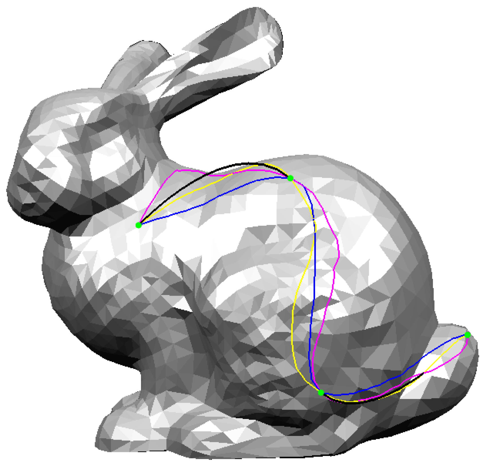
where $B_i^3\left(t\right)=\left(\begin{array}{c}3\\ i\end{array}\right){(1-t)}^{3-i}{t}^i$ is the ith Bernstein polynomial of degree 3, defined on $t\in [0,1]$. There exist several considerations when applying the Hermite interpolation scheme to a triangular mesh. The above equation involves the addition of a tangent vector to a point, which determines the intermediate control points. In general, these control points are not on a triangular mesh; thus, the generated interpolation curve also is not. Figure 1 shows the Hermite spline curve (in black) that interpolates four mesh points (in green). The Hermite spline curve is constructed by Equation (1) without considering the Bunny model and thus they do not lie on the model; the curve segment between second and third points penetrates the model.

Figure 1. Geodesic Hermite spline curve (in blue), Hermite spline curve (in black) and their projections onto the Bunny model (in pink and yellow).

A simple approach based on projection can be employed to ensure that the generated curve is laid on a triangular mesh. In Figure 1, the pink and yellow curves show the results of projecting the Hermite spline curve (in black) onto the Bunny model in two different viewing directions. Depending on the projection direction, different curves are obtained, and an invalid projection may occur when there is no intersection between the curve and the model. Consequently, this approach is not suitable for constructing an interpolation curve on a triangular mesh.

To resolve this limitation and construct consistent interpolation curves, it is necessary to define appropriate operations between points and vectors on a triangular mesh such as the addition of a vector to a point in (1). For this, the concept of the straightest geodesic that is a straight line from a mesh point in a given direction is employed [10]. The shortest geodesic between two points is approximated by the straightest geodesic that defines a geodesic vector on a triangular mesh.

In this paper, a simple and effective method is presented for constructing a Hermite spline curve that interpolates given points on a triangle mesh by combining previous methods [7,8,10]. The blue curve in Figure 1 shows the geodesic Hermite spline curve generated using the proposed method. The resulting curve is smooth and guaranteed to be on a triangular mesh while interpolating the given mesh points (in green). The main contributions of the method are summarized as follows:

• Geometric operations between points and vectors in Euclidean space are extended to those on a triangular mesh by leveraging the shortest geodesic with the straightest geodesic. These operations play an important role in constructing an interpolation curve on a triangular mesh.
• The method is simple to implement and easy to use because the conventional Hermite interpolation scheme is followed, except that a tangent vector in (1) is replaced with a geodesic vector and the related operations are defined on a triangular mesh.
• The method generates a geodesic Hermite spline curve that lies exactly on a triangular mesh while interpolating the given mesh points. To the best of our knowledge, our method is a new approach to solving this problem and compared with common projection methods, the proposed method guarantees consistent results and robustness. Moreover, the generated curve exhibits a symmetry property, i.e., the same interpolation curve is obtained if the mesh points are specified in the reverse order.

The remainder of this paper is organized as follows. In Section 2, some related work on the shortest geodesic and the straightest geodesic on a triangular mesh is reviewed, and the appropriate geometric operations needed for constructing Hermite spline curve on a triangular mesh are introduced in Section 3. In Section 4, the construction of Hermite spline curve by combining the conventional Hermite interpolation scheme with new geodesic operations is explained. In Section 5, the effectiveness of the proposed method is demonstrated by showing several examples of interpolation curves on triangular meshes. Finally, the conclusions and suggested future research are provided in Section 6.

2. Related Work

The aim is to construct piecewise smooth curves on a triangular mesh while interpolating the given points on the mesh. The simplest ones are the connected polylines on the mesh passing through the given points. If one wants to find effective ones with minimum length, the polylines become the shortest geodesics. In this section, previous work directly related to the focus of this paper is reviewed, including geodesic computation and its extension to the geodesic Bézier curve on a triangular mesh.

The shortest path between a pair of points in a plane is the line segment connecting them, but the algorithm must be extended to a Riemann manifold to obtain the shortest path on the three-dimensional mesh [9]. Many geometric problems can be solved efficiently by determining the shortest geodesic between a pair of points on the mesh. Therefore, much research [11,12,13,14] has been conducted on this topic, increasing the efficiency and accuracy of the computation algorithms.

Kimmel et al. [12] computed the shortest path from a triangular mesh by extending fast marching method to the triangular domain. The Mitchell–Mount–Papadimitriou (MMP) [13] and Chen-Han (CH) [11] algorithms are representative methods for computing the shortest geodesic on a polygonal mesh. Both are based on the subdivision of polyhedral surfaces and the continuous Dijkstra algorithm, with the MMP algorithm having $O\left(n^{2}logn\right)$ and the CH algorithm having $O\left(n^2\right)$ of time complexity. Surazhsky et al. [15] implemented the MMP algorithm and presented a faster way to find solutions by approximating the geodesic path. Xin et al. [16] significantly reduced the time and space complexity of the CH algorithm by eliminating unnecessary windows using current estimates of distances to the vertex and maintaining priority queues, as with the Dijkstra algorithm.

Polthier et al. [10,17] introduced a new type of geodesic on a polyhedral surface, called a straightest geodesic against the concept of the local shortest geodesic. The straightest geodesic is a straight line from a mesh point in a given direction. Computing the straightest geodesic can be considered an initial value problem with a unique solution, whereas the shortest geodesic solves the boundary value problem of finding the shortest path between two endpoints. If the straightest geodesic only passes through the edges, it is equivalent to the shortest geodesic. The straightest geodesic finds an optimal direction that minimizes the geodesic curvature when it meets a mesh vertex. The computation of the straightest geodesic is detailed in Section 3.

There have been many other studies on geodesic computation on a polygonal mesh [18,19,20,21]. Cheng et al. [18] constructed a smooth surface that approximates a polygonal mesh and computed a geodesic curve on the surface by solving a first-order ordinary differential equation of tangent vector. The discrete geodesic is then obtained by projecting the geodesic curve on the smooth surface onto the polygonal mesh. Lawonn et al. [19] proposed a method for smoothing polylines on a triangular mesh based on local reduction in geodesic curvature and made it possible for users to adjust their proximity to be the straightest geodesic. Qin et al. [20] proposed scenarios for effective window propagation and pruning, and developed triangle-oriented region growing techniques to reduce computational costs and memory usage significantly. Sharp et al. [21] presented a technique for calculating a geodesic on polyhedral surfaces by repeatedly performing edge flips based on the Delaunay flip algorithm [22,23]. As previous study showed [24], research on the shortest and straightest geodesic has continued until recently. In this paper, the straightest geodesic is used to represent a vector on a triangular mesh, and then the related operations between points and vectors on a triangular mesh are extended. Based on these operations, smooth interpolation curves on a triangular mesh can easily be obtained using the conventional Hermite interpolation scheme without significant modification.

Because the shortest geodesics show only $C^0$ continuity at junction points, they are not sufficient for smoothly interpolating points on a triangular mesh. To overcome this limitation and generate a smooth curve on a manifold or triangular mesh, Park et al. [9] generalized the de Casteljau algorithm in $SE\left(3\right)$ (special Euclidean group) and interpolated keyframes using Bézier curves. Their method is theoretically sound and excellent, but it cannot be applied directly to a polygonal mesh because it depends on the exponential and logarithmic maps between a manifold and its tangent space at identity. For practical usage, Martínez et al. [8] introduced a geodesic Bézier curve defined on a triangular mesh. They extended the de Casteljau algorithm in a triangular mesh by employing geodesic linear interpolation and generated a Bézier curve lying exactly on the domain mesh. In this study, the geodesic Bézier curve is further extend to geodesic Hermite spline curves to interpolate given points on a triangular mesh smoothly.

3. Geodesic Operations on Mesh

Computing a geodesic Hermite spline curve on a triangular mesh requires extended operations between the points and vectors on the mesh. In this section, these operations which include (i) the definition of a geodesic vector, (ii) subtraction between a pair of points, and (iii) parallel translation of a geodesic vector over the mesh, are defined.

3.1. Geodesic Vector on Mesh

Given a triangular mesh $\mathbb{M}$, let p be a point on a triangle $f\in \mathbb{M}$ and $\mathbf{v}$ be a vector in the tangent space $T_{\mathbf{p}}\mathbb{M}$. A “geodesic vector”, denoted by ${\stackrel{⌢}{\mathbf{v}}}_{\mathbf{p}}$ on $\mathbb{M}$ is defined as the straightest geodesic proposed by Polthier et al. [10]. A straightest geodesic is a directed polyline on $\mathbb{M}$, which emanates from $\mathbf{p}$ in direction $\mathbf{v}$. Computing the straightest geodesic, also known as “geodesic tracing”, can be summarized as follows.

• Compute the intersection point ${\mathbf{p}}^{\prime }$ of line $\mathbf{p}+t\mathbf{v}$ with the edge of the triangle f containing $\mathbf{p}$.
• Determine the next straight direction ${\mathbf{v}}^{\prime }$ by unfolding the adjacent triangle that shares the intersecting edge into a common plane.
• Repeat steps (1) and (2) by setting $\mathbf{p}={\mathbf{p}}^{\prime }$ and $\mathbf{v}={\mathbf{v}}^{\prime }$ until the length of the geodesic is equal to $\parallel \mathbf{v}\parallel$.

Figure 2 shows the geodesic vector ${\stackrel{⌢}{\mathbf{v}}}_{\mathbf{p}}$ (in pink) generated by the geodesic tracing algorithm. Please note that geodesic tracing can be considered the discrete exponential map ${exp}_{\mathbf{p}}:T_{\mathbf{p}}\mathbb{M}\to \mathbb{M}$ defined by ${exp}_{\mathbf{p}}\left(\mathbf{v}\right)={\stackrel{⌢}{\mathbf{v}}}_{\mathbf{p}}$ and it is restricted in the local neighborhood of $\mathbf{p}$ to construct one-to-one correspondence (see the rightmost image in Figure 3).

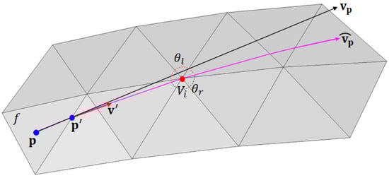
Figure 2. Geodesic vector ${\stackrel{⌢}{\mathbf{v}}}_{\mathbf{p}}$ on $\mathbb{M}$ computed by geodesic tracing.

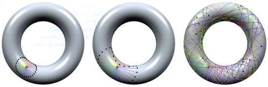
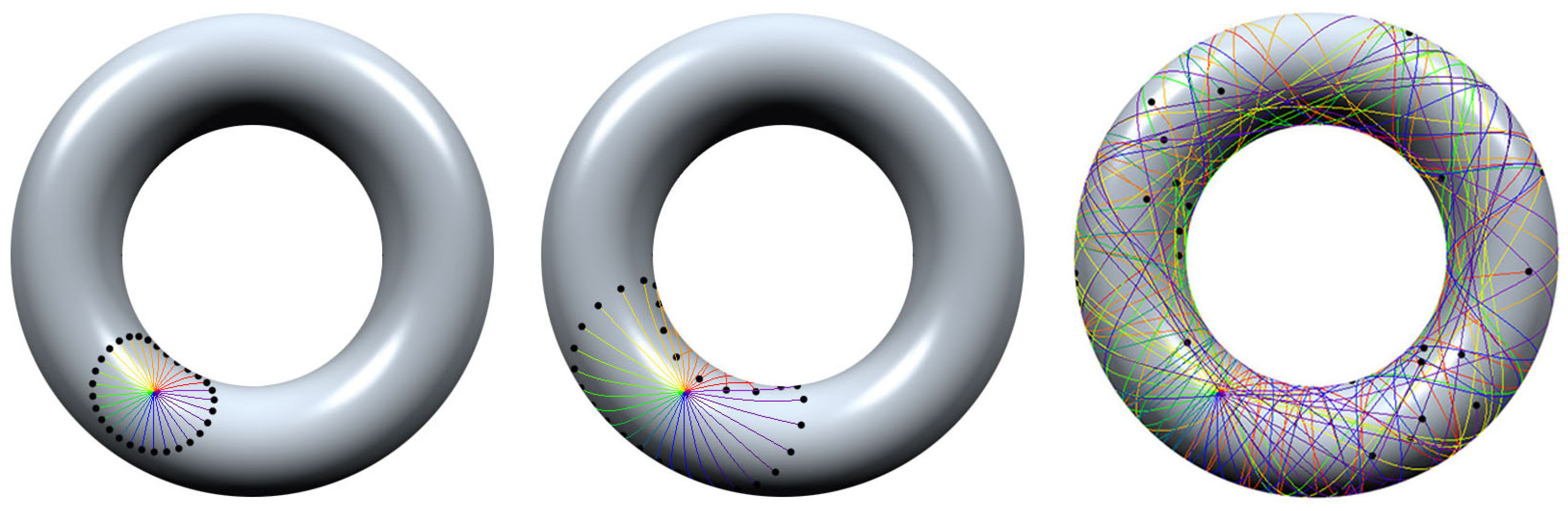
Figure 3. Geodesic vectors (straightest geodesics) on a torus model.

The angle sum ${\Theta }_i$ of a vertex $V_i$ is defined as:

$${\Theta }_i=\sum _{\forall f_j}{\theta }_i,$$

where ${\theta }_i$ is the interior angle at $V_i$ of triangle $f_j$ sharing $V_i$. Intuitively, ${\Theta }_i$ captures the flatness of the vertex, and $(2\pi -{\Theta }_i)$ is often used as a discrete analog of the Gaussian curvature. During geodesic tracing, the ambiguity of the unfolding triangle occurs when the intersection point ${\mathbf{p}}^{\prime }$ coincides with the mesh vertex $V_i$. In this case, a new direction ${\mathbf{v}}^{\prime }$ is chosen such that the geodesic curvature is minimized. More specifically, the direction that bisects the angle sum ${\Theta }_i$ is chosen as the new direction ${\mathbf{v}}^{\prime }$ while preserving the symmetry property of the straightest geodesic. In Figure 2, the geodesic vector meets vertex $V_i$; thus, the direction with symmetric angles (${\theta }_l={\theta }_r$) is chosen for the next direction. Figure 3 shows 30 straightest geodesics emanating from a single point on a torus model. As the figure goes to the right, it shows a longer and longer straightest geodesic with self-intersections possibly.

Scalar multiplication of a geodesic vector can be achieved by scaling its length, and the addition of two geodesic vectors, denoted by ${\stackrel{⌢}{\mathbf{v}}}_{\mathbf{p}}\oplus {\stackrel{⌢}{\mathbf{u}}}_{\mathbf{q}}$, can be computed by successive geodesic tracing if the endpoint of ${\stackrel{⌢}{\mathbf{v}}}_{\mathbf{p}}$ coincides with $\mathbf{q}$. Otherwise, it is necessary to move ${\stackrel{⌢}{\mathbf{u}}}_{\mathbf{q}}$ to ${\stackrel{⌢}{{\mathbf{u}}^{\prime }}}_{\mathbf{p}}$ over the mesh so that its start point becomes $\mathbf{p}$, as detailed in the following subsection. Here, the symbols ⊕ and ⊖ are used for addition and subtraction to distinguish them from those in Euclidean space. Please note that scalar multiplication combined with addition allows a linear combination of geodesic vectors, which produces a new geodesic vector on $\mathbb{M}$.

3.2. Geodesic Subtraction of Points

Let $\mathbf{p}$ and $\mathbf{q}$ be points on a triangular mesh $\mathbb{M}$. In Euclidean space, subtraction of $\mathbf{p}$ from $\mathbf{q}$ yields a vector that does not lie on the mesh in general. However, based on the definition of a geodesic vector on $\mathbb{M}$, subtraction of $\mathbf{p}$ from $\mathbf{q}$ should result in a geodesic vector from $\mathbf{p}$ to $\mathbf{q}$. In this section, the subtraction of points on a triangular mesh, equivalent to, the addition of a geodesic vector to a point, is defined.

For this, we employ the shortest geodesic from p to q, denoted by $\stackrel{⌢}{\mathbf{pq}}$. As mentioned in Section 2, there exist many efficient algorithms for geodesic computation on a polygonal mesh. Here, the shortest geodesic is computed by propagating the geodesic distance field and then back tracing using the distance field [13,15]. Figure 4 shows the geodesic distance field propagated from a source point $\mathbf{p}$ and the shortest geodesic (in pink) to the target point q. Alternatively, other methods [11,12,18,19,20,21] can be replaced to improve the computational efficiency and accuracy.

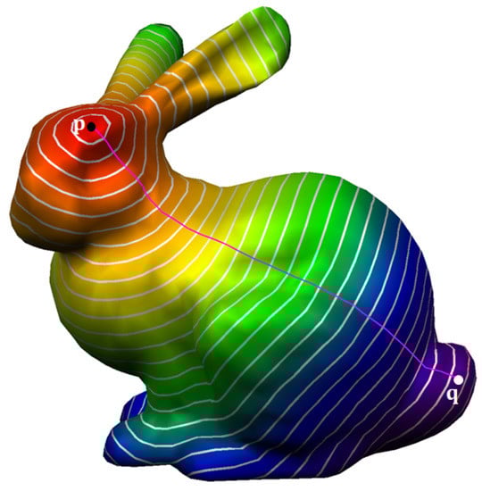
Figure 4. Shortest geodesic between two points on the Bunny model.

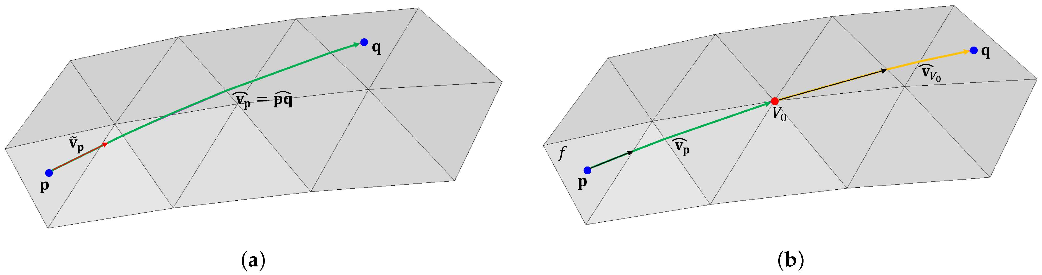
In general, the shortest geodesic consists of a single straightest geodesic or a sequence of straightest geodesics connected at the saddle vertex [11,13] which is a vertex $V_i$ with ${\Theta }_i>2\pi$. If the shortest geodesic $\stackrel{⌢}{\mathbf{p}\mathbf{q}}$ consists of a single straightest geodesic, or equivalently passes through only edges, it can be represented by a single geodesic vector ${\stackrel{⌢}{\mathbf{v}}}_{\mathbf{p}}$ as:

$$\stackrel{⌢}{\mathbf{p}\mathbf{q}}={\stackrel{⌢}{\mathbf{v}}}_{\mathbf{p}}=d_g(\mathbf{p},\mathbf{q}){\tilde{\mathbf{v}}}_{\mathbf{p}},$$

where $d_g(\mathbf{p},\mathbf{q})$ is the length of $\stackrel{⌢}{\mathbf{p}\mathbf{q}}$, and ${\tilde{\mathbf{v}}}_{\mathbf{p}}\in T_{\mathbf{p}}\mathbb{M}$ is the normalized tangent vector from p to the intersection of $\stackrel{⌢}{\mathbf{p}\mathbf{q}}$ with the edge of the triangle containing $\mathbf{p}$—see Figure 5a.

Figure 5. Subtraction between $\mathbf{p}$ and $\mathbf{q}$ results in (a) a single straightest geodesic and (b) two geodesic vectors joining at a vertex $V_i$.

If the shortest geodesic $\stackrel{⌢}{\mathbf{p}\mathbf{q}}$ passes through the saddle vertices $V_k (k=1,\cdots ,n)$, it cannot be represented by a single geodesic vector, but the sum of the geodesic vectors as follows:

$$\stackrel{⌢}{\mathbf{p}\mathbf{q}}={\stackrel{⌢}{\mathbf{v}}}_{\mathbf{p}}\oplus {\stackrel{⌢}{{\mathbf{v}}_1}}_{V_1}\oplus \cdots \oplus {\stackrel{⌢}{{\mathbf{v}}_n}}_{V_n}.$$

Figure 5b shows an example of the shortest geodesic, consisting of two geodesic vectors connected at the saddle vertex $V_0$. In such case, it is possible to retain all geodesic vectors to represent the shortest geodesic exactly. However, such case rarely occurs and thus approximation to $\stackrel{⌢}{\mathbf{p}\mathbf{q}}$ is taken by selecting the first geodesic vector ${\stackrel{⌢}{\mathbf{v}}}_{\mathbf{p}}$ for a practical usage. Finally, the subtraction of p from q is defined as the geodesic vector ${\stackrel{⌢}{\mathbf{v}}}_{\mathbf{p}}$ and the following notation is used to distinguish it from one in Euclidean space:

$$\mathbf{q}\ominus \mathbf{p}={\stackrel{⌢}{\mathbf{v}}}_{\mathbf{p}} \mathrm{or} \mathbf{p}\oplus {\stackrel{⌢}{\mathbf{v}}}_{\mathbf{p}}=\mathbf{q}.$$

3.3. Parallel Translation of Vector

Let q be a point and ${\stackrel{⌢}{\mathbf{v}}}_{\mathbf{p}}$ be a geodesic vector on a triangular mesh $\mathbb{M}$. Because the start position of ${\stackrel{⌢}{\mathbf{v}}}_{\mathbf{p}}$ does not coincide with q, one cannot add ${\stackrel{⌢}{\mathbf{v}}}_{\mathbf{p}}$ to q directly. To make this operation allowable, it is necessary to move ${\stackrel{⌢}{\mathbf{v}}}_{\mathbf{p}}$ to ${\stackrel{⌢}{{\mathbf{v}}^{\prime }}}_{\mathbf{q}}$ so that it starts from q. In this section, the geodesic operations of points and vectors in $\mathbb{M}$ are completed by introducing the parallel translation of a geodesic vector over $\mathbb{M}$.

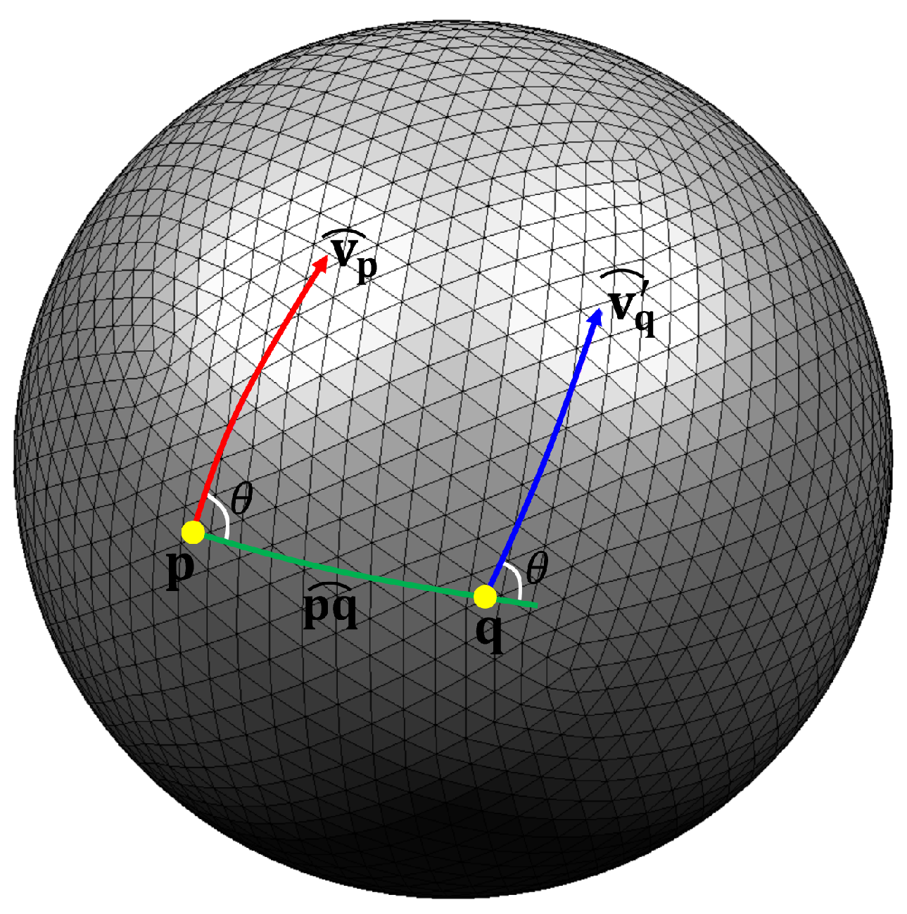
To move ${\stackrel{⌢}{\mathbf{v}}}_{\mathbf{p}}$ to $\mathbf{q}$ in parallel, the shortest geodesic $\stackrel{⌢}{\mathbf{p}\mathbf{q}}$ is used again. Let $\theta$ be the angle between ${\stackrel{⌢}{\mathbf{v}}}_{\mathbf{p}}$ and $\stackrel{⌢}{\mathbf{p}\mathbf{q}}$ (see Figure 6). One extends $\stackrel{⌢}{\mathbf{p}\mathbf{q}}$ by geodesic tracing and determines a unit vector ${\tilde{\mathbf{v}}}^{\prime }\in T_{\mathbf{q}}\mathbb{M}$ such that the extended $\stackrel{⌢}{\mathbf{p}\mathbf{q}}$ and ${\tilde{\mathbf{v}}}^{\prime }$ make an angle $\theta$. Finally, the parallel translation of ${\stackrel{⌢}{\mathbf{v}}}_{\mathbf{p}}$ to q, denoted by ${\stackrel{⌢}{{\mathbf{v}}^{\prime }}}_{\mathbf{q}}$, can be computed as follows:

$${\stackrel{⌢}{{\mathbf{v}}^{\prime }}}_{\mathbf{q}}=\parallel \mathbf{v}\parallel {\tilde{\mathbf{v}}}_{\mathbf{q}}^{\prime }.$$

Figure 6. Parallel translation of ${\stackrel{⌢}{\mathbf{v}}}_{\mathbf{p}}$ to ${\stackrel{⌢}{{\mathbf{v}}^{\prime }}}_{\mathbf{q}}$ using the shortest geodesic $\stackrel{⌢}{\mathbf{p}\mathbf{q}}$.

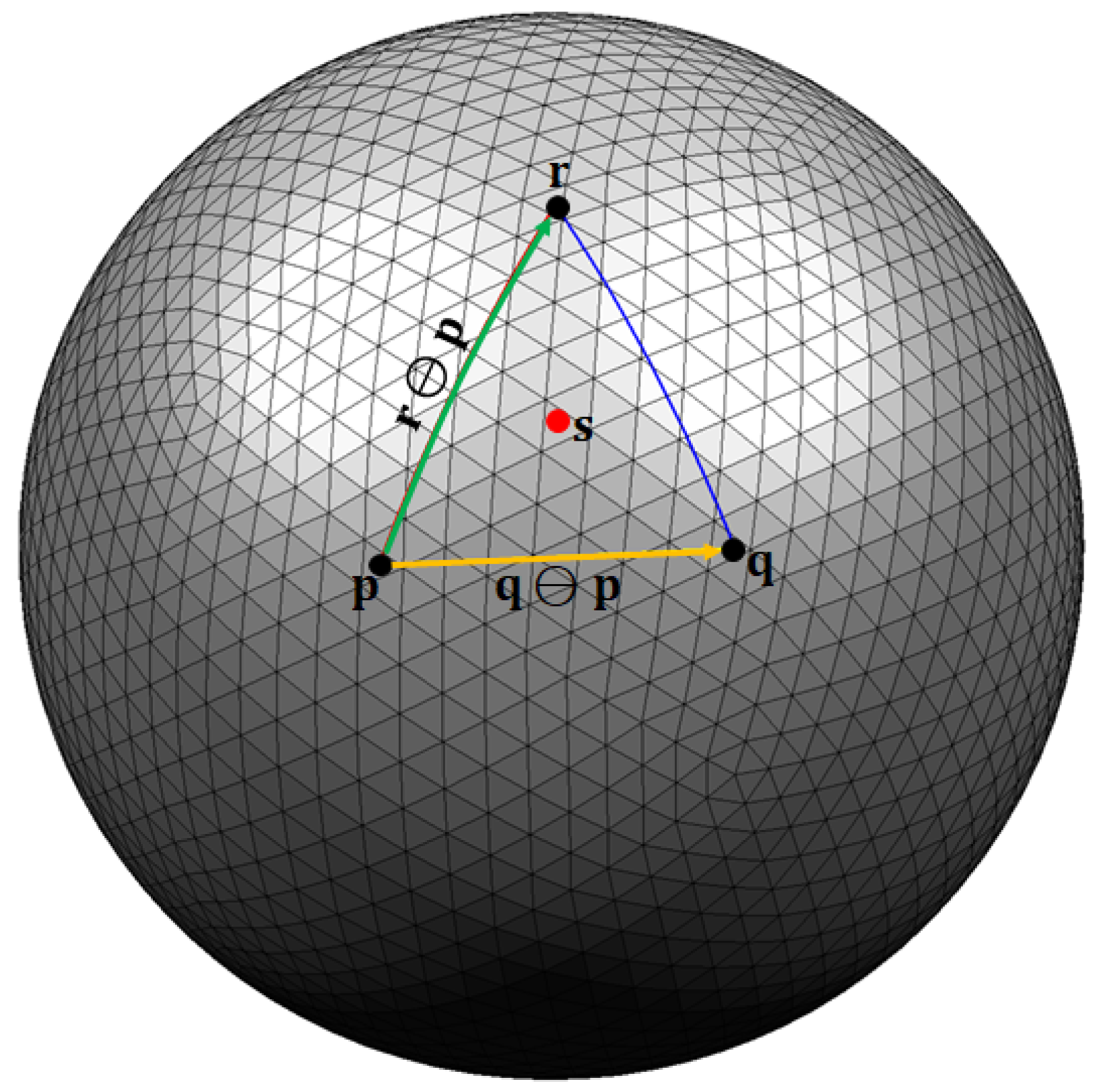
Intuitively, parallel translation of a geodesic vector on a triangular mesh is achieved by moving the geodesic vector while maintaining the angle formed by the shortest geodesic. Figure 6 illustrates the translation of a geodesic vector over a sphere model. The geodesic operations for points and vectors make it possible to perform algebraic computations on a triangular mesh, such as a linear combination of vectors and a convex combination of points. For example, Figure 7 shows the centroid $\mathbf{s}=\frac{\mathbf{p}+\mathbf{q}+\mathbf{r}}{3}$ of triangle $\Delta \mathbf{p}\mathbf{q}\mathbf{r}$ on a sphere, which can be computed by the geodesic operations as follows:

$$\mathbf{s}=\mathbf{p}\oplus \frac{1}{3}(\mathbf{q}\ominus \mathbf{p})\oplus \frac{1}{3}(\mathbf{r}\ominus \mathbf{p}).$$

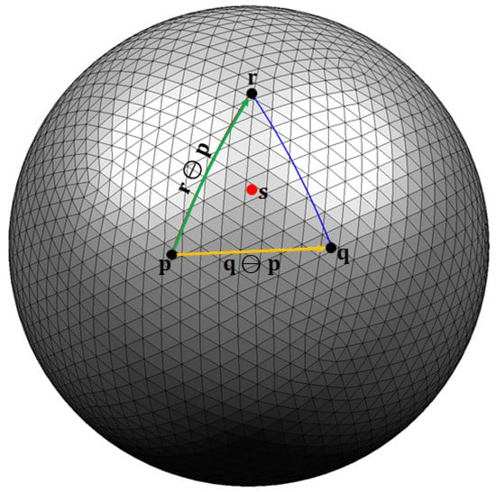
Figure 7. Centroid of a triangle $\Delta \mathbf{p}\mathbf{q}\mathbf{r}$ effectively computed by geodesic operations on a sphere.

4. Geodesic Hermite Spline Curve on Mesh

Now, an interpolation curve on a triangular mesh can be created using the geodesic operations introduced in the previous section. First, the interpolation parameters are determined by the geodesic length between consecutive input points. Second, the tangent vector for each point is computed by subtracting of consecutive points and third, the intermediate control points for each Bézier curve are computed by appropriate geodesic operations. Finally, the geodesic Hermite spline curve consists of a set of cubic Bézier curves generated by this method.

4.1. Hermite Spline Curve

The method is based on Hermite interpolation. Therefore, first, the conventional Hermite spline curve is summarized. Given two points ${\mathbf{p}}_0$ and ${\mathbf{p}}_1$, and their tangent vectors ${\mathbf{v}}_0$ and ${\mathbf{v}}_1$, the Hermite interpolation curve $C\left(u\right)$ defined on $u\in [a,b]$ while satisfying $C\left(a\right)={\mathbf{p}}_0,C\left(b\right)={\mathbf{p}}_1$ and $C^{\prime }\left(a\right)={\mathbf{v}}_0,C^{\prime }\left(b\right)={\mathbf{v}}_1$ can explicitly be constructed as:

$$C\left(u\right)={\mathbf{p}}_0{H}_0^3\left(t\right)+(b-a){\mathbf{v}}_0{H}_1^3\left(t\right)+(b-a){\mathbf{v}}_{\mathbf{1}}{H}_2^3\left(t\right)+{\mathbf{p}}_1{H}_3^3\left(t\right),$$

where $H_i^3\left(t\right),0\le t\left(=\frac{u-a}{b-a}\right)\le 1$ is the $i^{\mathrm{th}}$ Hermite basis function defined as follows:

$$\begin{array}{c}{H}_0^3\left(t\right)=2t^3-3t^2+1=B_0^3\left(t\right)+B_1^3\left(t\right),\hfill \\ H_1^3\left(t\right)=t^3-2t^2+t=\frac{1}{3}{B}_1^3\left(t\right),\hfill \\ H_2^3\left(t\right)=t^3-t^2=-\frac{1}{3}{B}_2^3\left(t\right),\hfill \\ H_3^3\left(t\right)=-2t^3+3t^2=B_2^3\left(t\right)+B_3^3\left(t\right).\hfill \end{array}$$

(2)

Based on the decomposition of Hermite basis functions $H_i^3\left(t\right)$ into Bernstein ones $B_i^3\left(t\right)$, the interpolation curve $C\left(u\right)$ can be represented by a cubic Bézier curve as:

$$C\left(u\right)={\mathbf{b}}_0{B}_0^3\left(t\right)+{\mathbf{b}}_1{B}_1^3\left(t\right)+{\mathbf{b}}_2{B}_2^3\left(t\right)+{\mathbf{b}}_3{B}_3^3\left(t\right),$$

where $0\le t\left(=\frac{u-a}{b-a}\right)\le 1$ and the control points are determined as follows:

$$\begin{array}{c}{\mathbf{b}}_0={\mathbf{p}}_0,\hfill \\ {\mathbf{b}}_1={\mathbf{p}}_0+\frac{b-a}{3}{\mathbf{v}}_0,\hfill \\ {\mathbf{b}}_2={\mathbf{p}}_1-\frac{b-a}{3}{\mathbf{v}}_1,\hfill \\ {\mathbf{b}}_3={\mathbf{p}}_1.\hfill \end{array}$$

(3)

In this paper, a Bézier form (3) for a Hermite curve is employed because its intermediate control points ${\mathbf{b}}_1$ and ${\mathbf{b}}_2$ can be handled efficiently by the geodesic operations defined in the previous section. By applying the Hermite interpolation method to a pair of points ${\mathbf{p}}_i$ and ${\mathbf{p}}_{i+1}$, and their tangent vectors ${\mathbf{v}}_i$ and ${\mathbf{v}}_{i+1}$, one can construct a Hermite spline curve with $C\left(u_i\right)={\mathbf{p}}_i$ and $C^{\prime }\left(u_i\right)={\mathbf{v}}_i$, where $u_i$ is an interpolation parameter for ${\mathbf{p}}_i$.

4.2. Interpolation Parameters

In general, interpolation parameters $u_i$ and tangent vectors ${\mathbf{v}}_i$ are not given; thus, it is necessary to determine them from given points ${\mathbf{p}}_0,{\mathbf{p}}_1,\cdots ,{\mathbf{p}}_n$. Common choices for interpolation parameters of a Hermite spline curve include uniform, chord length (chordal), and centripetal methods [25]. The chordal or centripetal method can solve the problem of loops or self-intersections caused by uniform parameters [26]. Yuksel et al. [27] showed that the centripetal method has superior properties compared with other methods. Here, chordal and centripetal methods are both used, and their effects are compared in Section 5.

Given the points ${\mathbf{p}}_0,{\mathbf{p}}_1,\cdots ,{\mathbf{p}}_n$, the interpolation parameters can be determined as follows:

$$u_i=u_{i-1}+{\parallel {\mathbf{p}}_i-{\mathbf{p}}_{i-1}\parallel }^{\alpha } \mathrm{with} u_0=0.$$

The chord length and centripetal parameters are obtained when $\alpha =1$ and $\alpha =\frac{1}{2}$, respectively. To extend this method to the points on a triangular mesh, the Euclidean distance $\parallel ·\parallel$ should be replaced with the geodesic distance $d_g(·,·)$ as follows:

$$u_i=u_{i-1}+d_g{({\mathbf{p}}_i,{\mathbf{p}}_{i-1})}^{\alpha } \mathrm{with} u_0=0.$$

(4)

Figure 8 shows an example of the chordal parameters for four points on a sphere model using the geodesic distances.

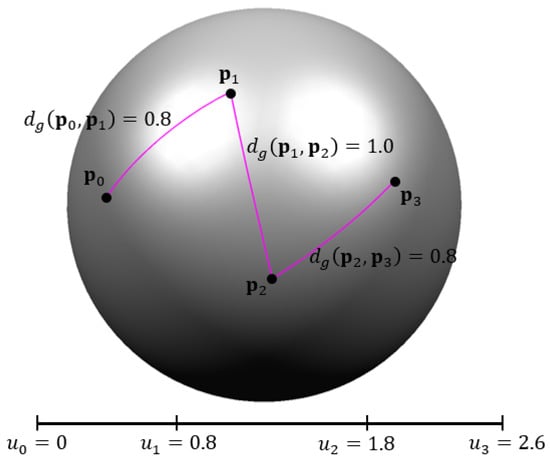
Figure 8. Determination of interpolation parameters by geodesic distance between consecutive points.

4.3. Geodesic Tangent Vectors

To construct a Hermite spline curve with $C^1$ continuity at $C\left(u_i\right)$ in Euclidean space, it is necessary to assign a tangent vector ${\mathbf{v}}_i$ to ${\mathbf{p}}_i$. Various methods for determining the tangent vectors of the Hermite spline curve exist, and the cardinal spline is a widely used technique. Let $u_i$ be the interpolation parameter for ${\mathbf{p}}_i$. The tangent vector ${\mathbf{v}}_i$ is computed as follows:

$${\mathbf{v}}_i=(1-c)\frac{{\mathbf{p}}_{i+1}-{\mathbf{p}}_{i-1}}{u_{i+1}-u_{i-1}},$$

(5)

where $c\in [0,1]$ is a tension parameter that controls the magnitude of the tangent vector. However, the tangent vector in (5) does not lie on a triangular mesh and therefore cannot be used for constructing an interpolation curve on a mesh.

In this paper, the Catmull–Rom spline is employed with $c=0.5$ [28] and the subtraction between two points is replaced with the geodesic operation to produce the “geodesic tangent vector” as follows:

$${\stackrel{⌢}{\mathbf{v}}}_{{\mathbf{p}}_i}=\frac{1}{2}\frac{{\mathbf{p}}_{i+1}\ominus {\mathbf{p}}_{i-1}}{u_{i+1}-u_{i-1}},$$

where the geodesic vector ${\mathbf{p}}_{\mathbf{i}+\mathbf{1}}\ominus {\mathbf{p}}_{\mathbf{i}-\mathbf{1}}$ moves to ${\mathbf{p}}_i$ by parallel translation (see Figure 9).

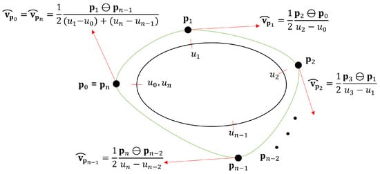
Figure 9. Determining tangent vector of the closed Hermite spline curve.

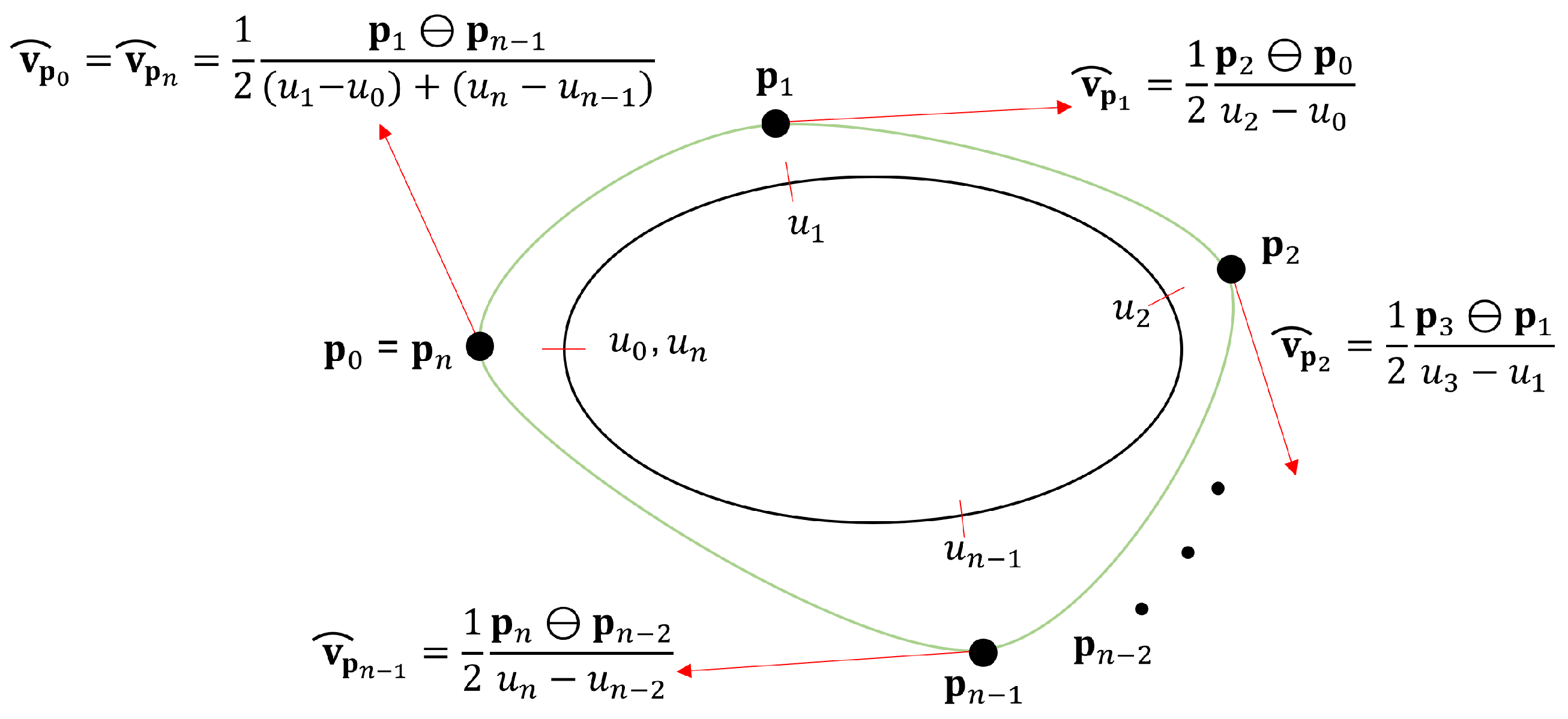
For an open Hermite spline curve, the geodesic tangent vectors ${\stackrel{⌢}{\mathbf{v}}}_{{\mathbf{p}}_0}$ and ${\stackrel{⌢}{\mathbf{v}}}_{{\mathbf{p}}_n}$ for the endpoints can be excluded or zero vectors. Here, zero vectors are assigned to the endpoints. A closed Hermite spline curve is quite useful for selecting a region bounded by the curve and, thus, is effectively used for such applications as mesh-cutting, texture mapping, and mesh hole filling. To construct a closed Hermite spline curve such that $C\left(u_0\right)=C\left(u_n\right)$, two endpoints should be identical, ${\mathbf{p}}_n={\mathbf{p}}_0$, and the common geodesic tangent vector should be assigned to both points as follows:

$${\stackrel{⌢}{\mathbf{v}}}_{{\mathbf{p}}_0}={\stackrel{⌢}{\mathbf{v}}}_{{\mathbf{p}}_n}=\frac{1}{2}\frac{{\mathbf{p}}_1\ominus {\mathbf{p}}_{n-1}}{(u_1-u_0)+(u_n-u_{n-1})}.$$

Figure 9 shows how to determine the geodesic tangent vector for each point ${\mathbf{p}}_i$ for constructing the closed Hermite spline curve.

4.4. Geodesic Hermite Spline Curve

Once the interpolation parameters $u_0,u_1,\cdots ,u_n$ and geodesic tangent vectors ${\stackrel{⌢}{\mathbf{v}}}_{{\mathbf{p}}_0},$ ${\stackrel{⌢}{\mathbf{v}}}_{{\mathbf{p}}_1},\cdots ,{\stackrel{⌢}{\mathbf{v}}}_{{\mathbf{p}}_n}$ have been obtained, one can construct a Hermite spline curve that interpolates given mesh points ${\mathbf{p}}_0,{\mathbf{p}}_1,\cdots ,{\mathbf{p}}_n$. The Hermite spline curve consists of piecewise $C^1$-continuous Bézier curves. Here, the focus is on a single geodesic Bézier curve $C_i\left(t\right)$ satisfying $C_i\left(u_i\right)={\mathbf{p}}_i$ and $C_i^{\prime }\left(u_i\right)={\stackrel{⌢}{\mathbf{v}}}_{{\mathbf{p}}_i}$. As mentioned, $C_i\left(t\right)$ can be represented by a cubic Bézier curve $C_i\left(t\right)={\sum }_{k=0}^3{\mathbf{b}}_k{B}_k^3\left(t\right)$, and the control points ${\mathbf{b}}_i$ can be computed as follows:

$$\begin{array}{c}{\mathbf{b}}_0={\mathbf{p}}_i,\hfill \\ {\mathbf{b}}_1={\mathbf{p}}_i\oplus \frac{u_{i+1}-u_i}{3} {\stackrel{⌢}{\mathbf{v}}}_{{\mathbf{p}}_i},\hfill \\ {\mathbf{b}}_2={\mathbf{p}}_{i+1}\ominus \frac{u_{i+1}-u_i}{3} {\stackrel{⌢}{\mathbf{v}}}_{{\mathbf{p}}_{i+1}},\hfill \\ {\mathbf{b}}_3={\mathbf{p}}_{i+1}.\hfill \end{array}$$

(6)

Because a cubic Hermite curve is used, both end control points ${\mathbf{b}}_0$ and ${\mathbf{b}}_3$ are simply set to be ${\mathbf{p}}_i$ and ${\mathbf{p}}_{i+1}$, respectively, and intermediate control points ${\mathbf{b}}_1$ and ${\mathbf{b}}_2$ are calculated by geodesic tangent vectors and constants related to the difference between interpolation parameters $u_i$ and $u_{i+1}$, as in Equation (6). Figure 10 shows how to determine the intermediate control points between interpolation points ${\mathbf{p}}_1$ and ${\mathbf{p}}_2$. The intermediate control points ${\mathbf{b}}_1$ and ${\mathbf{b}}_2$ are determined by the geodesic tangent vectors ${\mathbf{v}}_1$ and ${\mathbf{v}}_2$.

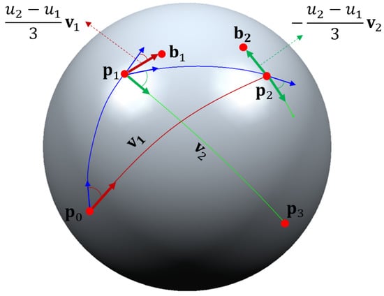
Figure 10. Determining intermediate control points in partial Bézier curves.

Equation (6) is equivalent to (3), except that the operations are replaced with geodesic ones—that is, the geodesic operations on a triangular mesh make it possible to reuse the conventional Hermite spline technique for constructing an interpolation curve on the mesh.

5. Experimental Results

The proposed method was implemented on a PC with an Intel i7-9700F CPU, 24.0-GB main memory, and an NVIDIA GeForce RTX 2060 graphics card, using the C++ language. The geodesic Hermite spline curve discussed can be used in various applications, including curve design on a polygonal mesh, as well as mesh-cutting and simulation of a moving object along the interpolation curves. The effectiveness of the method was demonstrated by designing several sophisticated curves on triangular meshes and applying them to various applications such as mesh-cutting, segmentation and simulation.

5.1. Hermite Spline Curves on Mesh

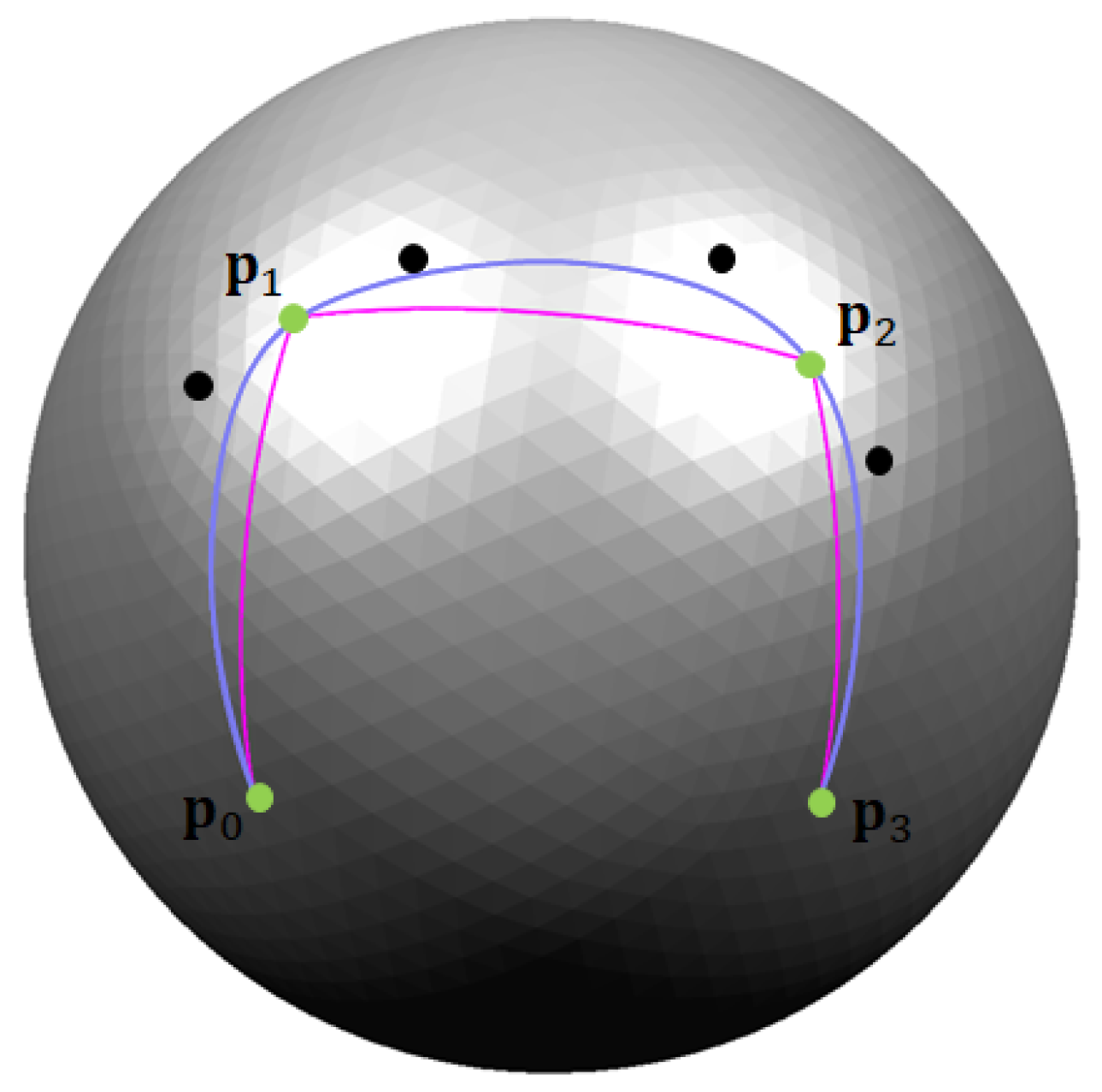
To create a geodesic Hermite spline curve, a user must select at least two points on a triangular mesh at runtime. Figure 11 shows four user-selected points (in green) on a sphere model and the shortest geodesics (in pink) between a pair of points. Although a sequence of shortest geodesics can be used for interpolating given points, they are inadequate for providing $C^1$-continuous curves. The Hermite spline curve interpolating four points is shown in blue, where three Bézier curves are joined with $C^1$ continuity. In this example, chordal parameters and Catmull–Rom splines were employed to determine the geodesic tangent vectors. The intermediate control points determined by the geodesic operations are shown in black. Given n mesh points, this method generates $(n-1)$ cubic Bézier curves with $C^1$ continuity. Please note that the generated curve shows a symmetry property, i.e., the same interpolation curve is obtained if the mesh points are specified in the reverse order.

Figure 11. Hermite spline curve interpolating four given mesh points.

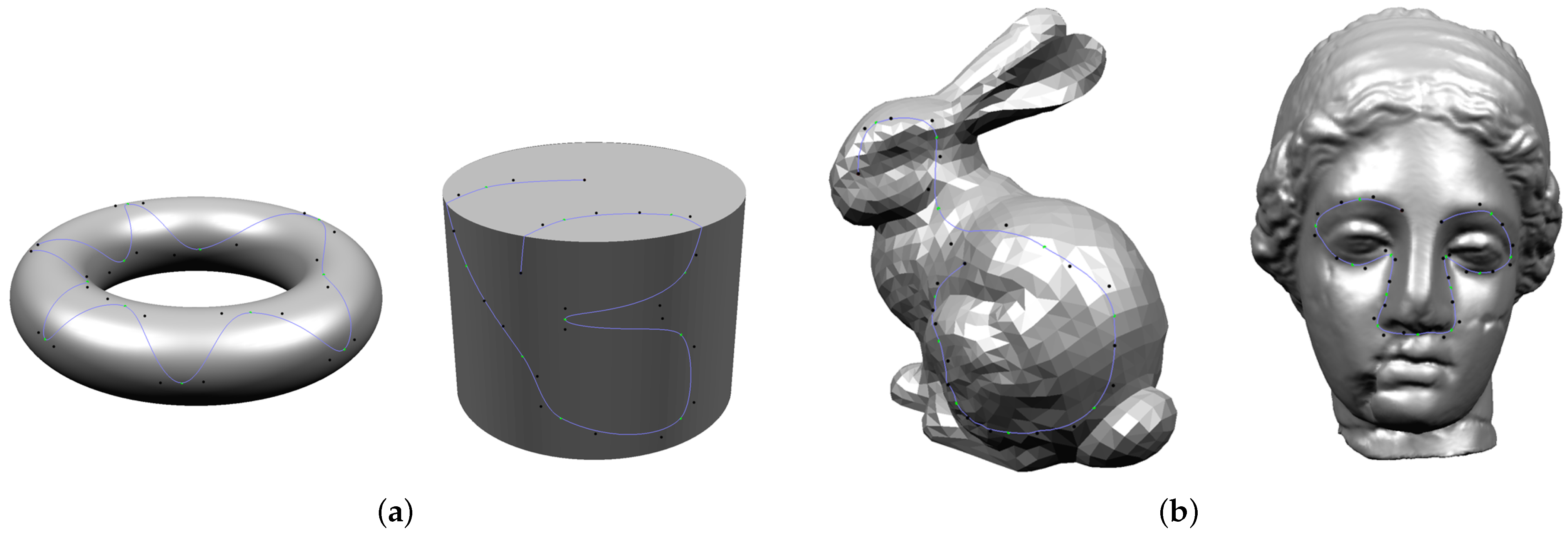
Figure 12a,b show additional examples of geodesic Hermite spline curves on various CAD models and 3D scanned models, respectively. As shown in these examples, the proposed method is quite useful and effective for creating smooth interpolation curves on various triangular meshes. The numbers of vertices and interpolation points are listed in the first and second rows in Table 1, and the time for constructing geodesic Hermite spline curves for each model is listed in the last row in Table 1, where sampling points on the interpolation curve is not included in the construction time.

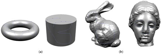
Figure 12. Geodesic Hermite spline curves on (a) CAD models and (b) 3D scanned meshes.

Table 1. Geometric information for test models.

Models	Sphere	Torus	Cylinder	Bunny	Igea
# of verts.	2562	9801	6956	2138	134,345
# of interp. pts.	4	13	12	9	15
Time (in ms)	2	44	25	10	110

The proposed technique shows a real-time performance for most of test examples presented in this paper. If the user moves an interpolation point to a new position, the method generates a new Hermite spline curve interpolating the new position in real time (see the Video S1).

5.2. Mesh-Cutting with Closed Curve

The selection of a region of interest, followed by cutting is one of the fundamental operations in geometric modeling and processing. In particular, a sophisticated boundary curve is required for mesh segmentation and partial texture mapping. The method provides an effective solution to these applications. By creating a closed Hermite spline curve, the user can select a region of interest on the model and cut the region with ease.

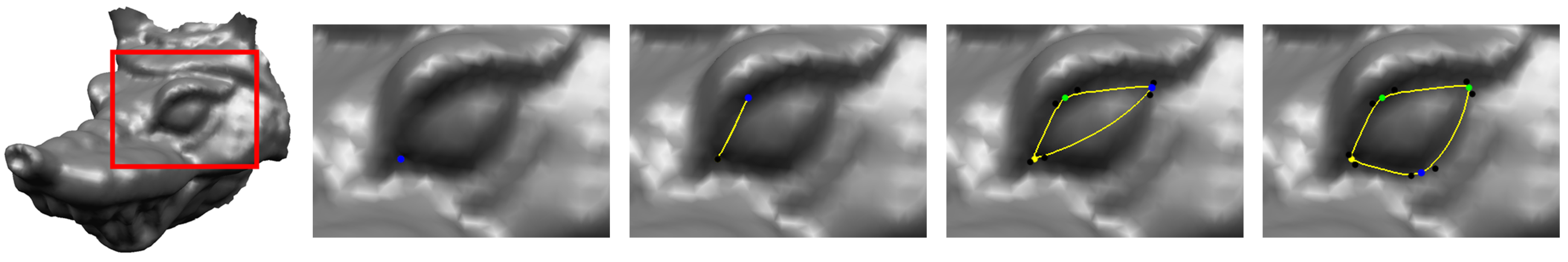
Figure 13 shows the process of generating a closed Hermite spline curve near the eye of the Armadillo model. Four interpolation points near the left eye region were selected interactively and the resulting interpolation curve was constructed to separate the eye of the Armadillo model. Figure 14a shows the selection of the left eye of the model using the closed interpolation curve and Figure 14b shows the result of cutting the selected region.

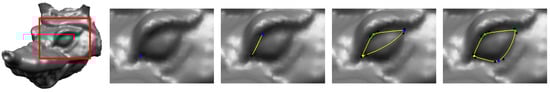
Figure 13. Process of generating a closed Hermite spline curve on the Armadillo model.

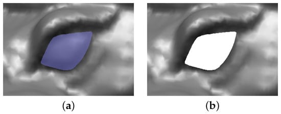
Figure 14. Selection followed by cut: (a) eye region of the Armadillo model is selected by a closed Hermite spline curve and (b) the selected region is cut by the generated curve.

5.3. Simulation

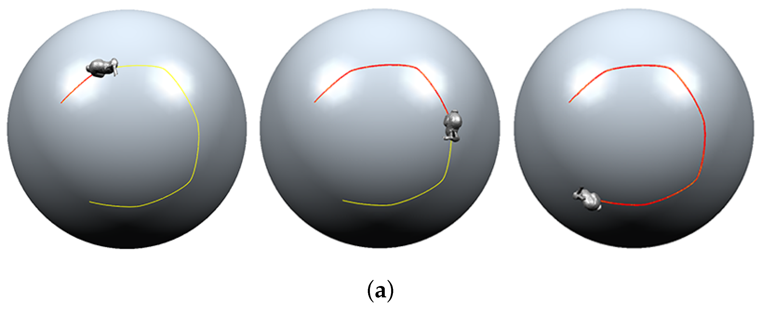
The Hermite spline curve on the mesh can also be used for the simulation of an object or camera moving along the generated path. Figure 15a shows the Bunny model moving along a curved path on a spherical model. In the figure, the yellow curve is the Hermite spline curve on the sphere, and the red curve indicates the path through which the Bunny model passed. Figure 15b shows the local axis of the curved paths on a sphere, Bunny and cylinder models, all of which are generated by the method presented.

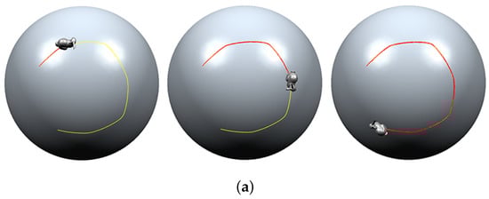
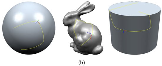
Figure 15. (a) Simulation of the Bunny model moving along the path on a sphere and (b) local axes of the curved paths on various models.

5.4. Control Parameters

Our technique provides the user with two parameters $\alpha$ in Equation (4) and c in Equation (5) for controlling the shape of the generated Hermite spline curve. In this section, the effects of these control parameters when creating a geodesic Hermite spline curve are discussed.

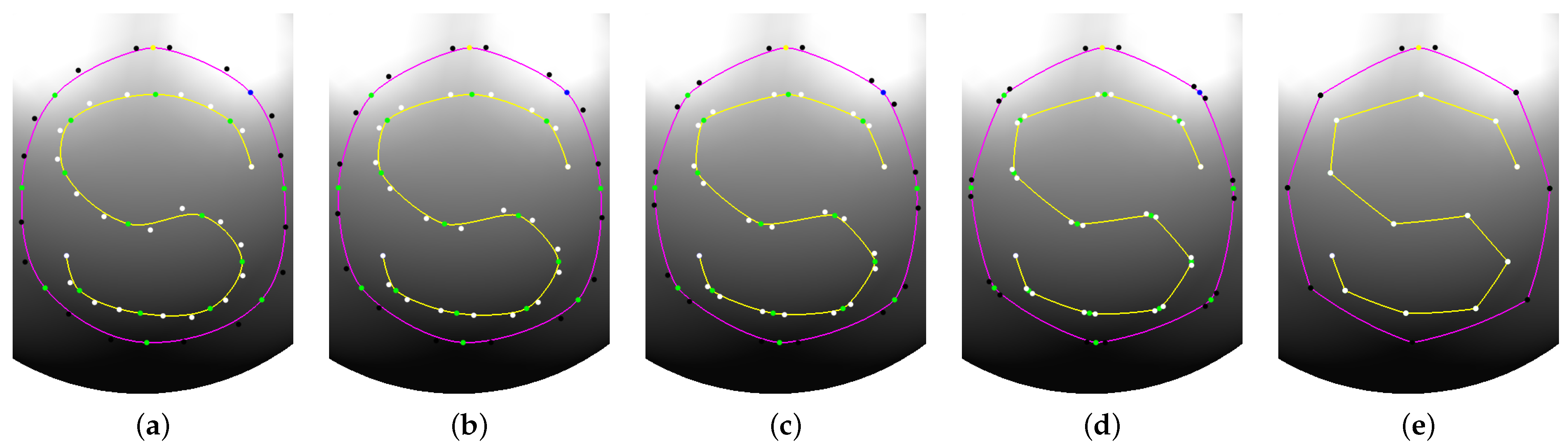
Figure 16 shows the effects of changing the tension parameter $c\in [0,1]$ in Equation (5). The tension parameter controls the length of the geodesic tangent vector, and therefore influences the sharpness of the generated curve at the interpolation points. In this example, 12 points are given for the open Hermite spline curve (in yellow) and 9 points are given for the closed Hermite spline curve (in pink). The interpolation parameters are computed by the chord length method for all tests. As the tension parameter increases, the generated Hermite spline curve approaches the shortest geodesic (see the Video S1).

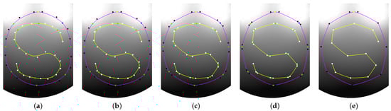
Figure 16. Hermite spline curves controlled by tension parameter: (a) $c=0$, (b) $c=0.25$, (c) $c=0.5$, (d) $c=0.75$ and (e) $c=1.0$.

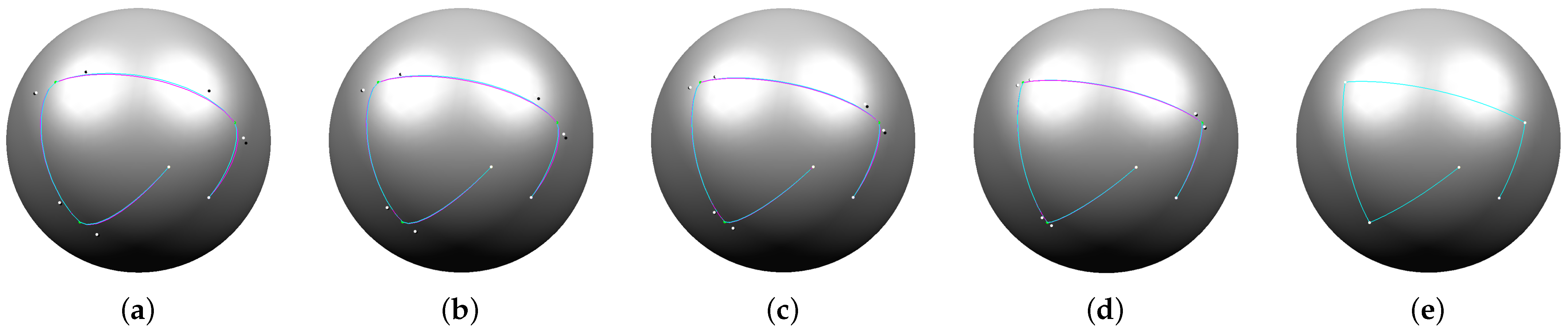
Figure 17 shows the effects of changing the control parameter $\alpha$ in Equation (4) which influences the interpolation parameters $u_i$, where pink curves are generated by centripetal parameter ($\alpha =0.5$) and blue ones are generated by chordal parameter ($\alpha =1$). Depending on the interpolation parameters of the given points, the method produces slightly different results. As the tension parameter increases, the two curves become identical. These examples demonstrate that our method follows the same control mechanism as the conventional Hermite spline curves in Euclidean space.

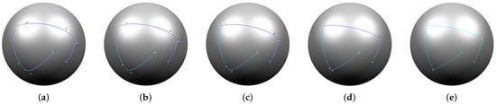
Figure 17. Two Hermite spline curves with $\alpha =0.5$ and $\alpha =1$ controlled by tension parameter: (a) $c=0$, (b) $c=0.25$, (c) $c=0.5$, (d) $c=0.75$ and (e) $c=1.0$.

6. Conclusions

An effective method for constructing a geodesic Hermite spline curve on a triangular mesh while interpolating the given mesh points was presented. To extend the conventional Hermite interpolation method to a triangular mesh, new geodesic operations between points and vectors on a triangular mesh were defined by using the concept of the shortest geodesic and straightest geodesic. The geodesic Hermite spline curve was constructed using the conventional Hermite interpolation method, except that the algebraic operations were replaced with the new geodesic operations.

The method is simple to implement and easy to use. A user simply selects the points on a triangular mesh, and then the interpolation curve is generated in real time. Moreover, the generated curve can be edited by simply moving the interpolation point to a new position interactively. In the experimental results, the effectiveness of the technique was demonstrated by showing several examples and applying the method to various applications.

In the current implementation, the subtraction of two points was approximated with a single geodesic vector, which can be improved by keeping all geodesic vectors. In future work, it is planned to apply the geodesic operations to other applications, such as computations of Voronoi diagram and medial axis bounded by geodesic curves on a polygonal model.

References

- Lee, H.; Kim, L.; Meyer, M.; Desbrun, M. Meshes on fire. In Computer Animation and Simulation; Springer: Vienna, Austria, 2001; pp. 75–84. [Google Scholar]
- Vekhter, J.; Zhuo, J.; Fandino, L.F.G.; Huang, Q.; Vouga, E. Weaving geodesic foliations. ACM Trans. Graph. (TOG) 2019, 38, 1–22. [Google Scholar] [CrossRef]
- Peyré, G.; Cohen, L. Geodesic computations for fast and accurate surface remeshing and parameterization. In Elliptic and Parabolic Problems; Birkhäuser: Basel, Switzerland, 2005; pp. 157–171. [Google Scholar]
- Lee, Y.; Lee, S.; Shamir, A.; Cohen-Or, D.; Seidel, H.P. Mesh scissoring with minima rule and part salience. Comput. Aided Geom. Des. 2005, 22, 444–465. [Google Scholar] [CrossRef]
- Kaplansky, L.; Tal, A. Mesh segmentation refinement. In Computer Graphics Forum; Blackwell Publishing Ltd.: Oxford, UK, 2019; Volume 28, pp. 1995–2003. [Google Scholar]
- Cohen, E.; Riesenfeld, R.F.; Elber, G. Geometric Modeling with Splines: An Introduction; CRC Press: New York, NY, USA, 2001. [Google Scholar]
- Farin, G.; Hansford, D. The Essentials of CAGD; CRC Press: Boca Raton, FL, USA, 2000. [Google Scholar]
- Morera, D.M.; Carvalho, P.C.; Velho, L. Modeling on triangulations with geodesic curves. Vis. Comput. 2008, 24, 1025–1037. [Google Scholar] [CrossRef]
- Park, F.C.; Ravani, B. Bézier curves on riemannian manifolds and lie groups with kinematics applications. J. Mech. Des. 1995, 117, 36–40. [Google Scholar] [CrossRef] [Green Version]
- Polthier, K.; Schmies, M. Straightest geodesics on polyhedral surfaces. In ACM SIGGRAPH 2006 Courses; Association for Computing Machinery: New York, NY, USA, 2006; pp. 30–38. [Google Scholar]
- Chen, J.; Han, Y. Shortest paths on a polyhedron. In Proceedings of the Sixth Annual Symposium on Computational Geometry, Berkley, CA, USA, 7–9 June 1990; pp. 360–369. [Google Scholar]
- Kimmel, R.; Sethian, J.A. Computing geodesic paths on manifolds. Proc. Natl. Acad. Sci. USA 1998, 95, 8431–8435. [Google Scholar] [CrossRef] [PubMed] [Green Version]
- Mitchell, J.S.; Mount, D.M.; Papadimitriou, C.H. The discrete geodesic problem. SIAM J. Comput. 1987, 16, 647–668. [Google Scholar] [CrossRef]
- Sharir, M.; Schorr, A. On shortest paths in polyhedral spaces. SIAM J. Comput. 1986, 15, 193–215. [Google Scholar] [CrossRef]
- Surazhsky, V.; Surazhsky, T.; Kirsanov, D.; Gortler, S.J.; Hoppe, H. Fast exact and approximate geodesics on meshes. ACM Trans. Graph. (TOG) 2005, 24, 553–560. [Google Scholar] [CrossRef] [Green Version]
- Xin, S.Q.; Wang, G.J. Improving chen and han’s algorithm on the discrete geodesic problem. ACM Trans. Graph. (TOG) 2009, 28, 1–8. [Google Scholar] [CrossRef]
- Polthier, K.; Schmies, M. Geodesic flow on polyhedral surfaces. In Data Visualization’99; Springer: Vienna, Austria, 1999; pp. 179–188. [Google Scholar]
- Cheng, P.; Miao, C.; Liu, Y.J.; Tu, C.; He, Y. Solving the initial value problem of discrete geodesics. Comput.-Aided Des. 2016, 70, 144–152. [Google Scholar] [CrossRef]
- Lawonn, K.; Gasteiger, R.; Rössl, C.; Preim, B. Adaptive and robust curve smoothing on surface meshes. Comput. Graph. 2014, 40, 22–35. [Google Scholar] [CrossRef]
- Qin, Y.; Han, X.; Yu, H.; Yu, Y.; Zhang, J. Fast and exact discrete geodesic computation based on triangle-oriented wave front propagation. ACM Trans. Graph. (TOG) 2016, 35, 1–13. [Google Scholar] [CrossRef] [Green Version]
- Sharp, N.; Crane, K. You can find geodesic paths in triangle meshes by just flipping edges. ACM Trans. Graph. (TOG) 2020, 39, 1–15. [Google Scholar] [CrossRef]
- Lawson, C.L. Software for c1 surface interpolation. In Mathematical Software; Academic Press: New York, NY, USA, 1977; pp. 161–194. [Google Scholar]
- Rivin, I. Euclidean structures on simplicial surfaces and hyperbolic volume. Ann. Math. 1994, 139, 553–580. [Google Scholar] [CrossRef]
- Alekseevsky, D. Shortest and straightest geodesics in sub-riemannian geometry. J. Geom. Phys. 2020, 155, 103713. [Google Scholar] [CrossRef]
- Lee, E.T. Choosing nodes in parametric curve interpolation. Comput.-Aided Des. 1989, 21, 363–370. [Google Scholar] [CrossRef]
- Dyn, N.; Floater, M.S.; Hormann, K. Four-point curve subdivision based on iterated chordal and centripetal parameterizations. Comput. Aided Geom. Des. 2009, 26, 279–286. [Google Scholar] [CrossRef]
- Yuksel, C.; Schaefer, S.; Keyser, J. Parameterization and applications of Catmull–rom curves. Comput.-Aided Des. 2011, 43, 747–755. [Google Scholar] [CrossRef] [Green Version]
- Catmull, E.; Rom, R. A class of local interpolating splines. In Computer Aided Geometric Design; Academic Press: New York, NY, USA, 1974; pp. 317–326. [Google Scholar]
Publisher’s Note: MDPI stays neutral with regard to jurisdictional claims in published maps and institutional affiliations. |
© 2021 by the authors. Licensee MDPI, Basel, Switzerland. This article is an open access article distributed under the terms and conditions of the Creative Commons Attribution (CC BY) license (https://creativecommons.org/licenses/by/4.0/).