Article

On the Controllability of a System Modeling Cell Dynamics Related to Leukemia

by
Ioan Ştefan Haplea
1,†,
Lorand Gabriel Parajdi
2,3,† and
Radu Precup
4,5,*,†
1
Department of Internal Medicine, Iuliu Haţieganu University of Medicine and Pharmacy, 400012 Cluj-Napoca, Romania
2
Department of Mathematics, West Virginia University, Morgantown, WV 26506, USA
3
Department of Mathematics, Babeş–Bolyai University, 400084 Cluj-Napoca, Romania
4
Institute of Advanced Studies in Science and Technology STAR-UBB, Babeş-Bolyai University, 400084 Cluj-Napoca, Romania
5
Tiberiu Popoviciu Institute of Numerical Analysis, Romanian Academy, 400015 Cluj-Napoca, Romania
*
Author to whom correspondence should be addressed.
These authors contributed equally to this work.
Symmetry 2021, 13(10), 1867; https://doi.org/10.3390/sym13101867
Submission received: 23 June 2021 / Revised: 11 August 2021 / Accepted: 19 August 2021 / Published: 3 October 2021
(This article belongs to the Special Issue Complex Systems and Its Applications)

Abstract

:
In this paper, two control problems for a symmetric model of cell dynamics related to leukemia are considered. The first one, in connection with classical chemotherapy, is that the evolution of the disease under treatment should follow a prescribed trajectory assuming that the drug works by increasing the cell death rates of both malignant and normal cells. In the case of the second control problem, as for targeted therapies, the drug is assumed to work by decreasing the multiplication rate of leukemic cells only, and the control objective is that the disease state reaches a desired endpoint. The solvability of the two problems as well as their stability are proved by using a general method of analysis. Some numerical simulations are included to illustrate the theoretical results and prove their applicability. The results can possibly be used to design therapeutic scenarios such that an expected clinical evolution can be achieved.
MSC:
34H05; 93B05

1. Introduction

1.1. Biological Background

Hematological malignancies were the first types of cancer for which chemotherapy was attempted and then refined [1]. The blood stem cell was the first stem cell ever discovered (reviewed in [2]), and the well-established developmental hierarchy of hematopoiesis allowed for its rigorous functional characterization. Leukemias were the first malignancies in which cancer stem cells were documented (reviewed in [3]).
Classical cancer chemotherapeutics have strong cell cycle dependence [4] and, unlike targeted therapies, act preferentially on cancer cells rather than on normal cells, mainly because of the higher division rate of cancer cells. Any normal cell line with a high turnover rate will be also affected to a degree, as is the case with the highly active normal hematopoietic cells in the bone marrow. From the point of view of chemotherapy, the population of leukemia cells (to eliminate) and the population of normal cells (to be spared) are pharmacologically much closer and harder to discriminate between than, say, a colon cancer entoured by normal colonic mucosa or a hepatocarcinoma surrounded by normal hepatic parenchyma [5]. This narrower error margin makes leukemias an ideal proving ground for models of safety in chemotherapy and highlights the need for an accurate control of therapy. The diffuse and homogenous distribution of leukemic infiltrate within the marrow of axial bones [6] simplifies the assumptions of pharmacokinetic models, eliminates confusion factors, and allows focus on the study on the antineoplastic effect itself.
Unlike in solid tumors, leukemic cells do not possess the intracellular and cell surfaces necessary for tumor cohesion. The cellular mass of leukemias is fluidic, lacking, to a degree [7], a fixed and meaningful positional relationship between individual cells. As such, the spatial aspects of tumorigenesis can be reasonably abstracted away, which renders leukemias, as in the case of other types of population dynamics, especially suited for modeling with systems of ordinary differential equations.
In our model, the chemotherapeutics are not represented directly (as a system variable); they are instead modeled as an effect on the growth rates and removal rates of cells. It is unclear how to modify such parameters in response to a drug, as there is a conceptual gap between individual cell models and global tumor models. Taking the case of the common anti-tumor drug Paclitaxel [8], its prime effect on the cell is mitotic arrest: the affected cell will stop dividing and often (but not always) suffer apoptotic death. The way to proceed from this point is dependent on opinion more than fact. One can model its effect as an increase in the tumor cell death rate (the most common way), or as a combination of growth rate decrease and death rate increase. Our first problem, considered in Section 3, concerns a hypothetical drug that acts by increasing solely the death rates of both malignant and normal cells, while for the second problem (Section 4), the drug is assumed to act only on the growth rate of malignant cells.
One can expect that one of the directions of improvement in cancer therapeutics in the near future will consist of treatment algorithms. At the limit, adjusting the drug delivery to a very fine-grained schedule (see Remark 1 (b)) means identifying a continuous change of one or more kinetic parameters so that a clinical evolution can be achieved. If this detailed level of control proves to be beneficial, chemotherapy could be delivered via solutions that are already in clinical practice, such as infusion pumps, either extracorporeal or implanted.
There are two metrics of control over the course of a disease, relating to the disease trajectory and to the disease endpoint, respectively. Traditionally, the endpoint refers to therapeutic efficiency (reduction of the leukemic burden below a set threshold, inducing remission, etc.) and the parcourse to therapeutic safety (such as the total amount of toxic chemotherapy to which the patient is exposed over the entire treatment time course). Still, the delegation of efficiency only to the endpoint criteria is limiting. The recognition of cancer as a dynamic disease makes it obvious that some critical aspects, such as the risk of relapse, can only be taken into account by an analysis of its full trajectory in time [9]. As an immediate example, if the total leukemic cell number is massive for the largest part of the treatment, then the probability of inducing drug resistance is greater, compared to the situation where the leukemic cell number is rapidly reduced from the onset, even if in both cases the treatment manages to bring the leukemic cell number down to the same final size.
Consequently, it may be desirable not only to reach a given endpoint but also to reach it along a specific route in the space of possible disease states, which is complex and only partially observable. We have formulated these two situations separately: one situation is where the dynamics matter as well as the endpoint, and the tumoral mass must decrease under treatment along a prespecified curve (the first control problem, Section 3), and the other situation is where only the end state is of interest (i.e., bringing the tumoral mass to a given low value; Section 4—the second control problem).
In the first case, the drug works by increasing the cell death rate, acts on both normal and leukemic cells, and can model any classical chemotherapy in exclusive use for any acute form of leukemia (myeloid or lymphoblastic). The case cannot apply, however, to the modern treatment of blast crises occurring in chronic myeloid leukemia (acute-like form), in which a targeted drug is used in addition to classical therapy.
In the second case, the drug works by decreasing the multiplication rate, acts on leukemic cells only, and models the effect of targeted therapies used in isolation. This case refers specifically to the chronic or accelerated phases of chronic myeloid leukemia, involving a targeted drug from the tyrosine kinase inhibitor family (TKI) (Imatinib, Dasatinib, Nilotinib, Bosutinib, Ponatinib). These drugs have only marginal toxicity on normal cells from the bone marrow, and a TKI is the single antileukemic treatment administered.
Note that an interesting application of the first control problem lies outside of the field of leukemia treatment. If we replace the “normal” and “malignant” cell populations with two—both normal—cell lineages, with different responses to a growth signal, the problem relates to bone marrow homeostasis. Some other applications of our control problems, or of some of their variants, to population dynamics in general could be also imagined.

1.2. Mathematical Model and Approach

Several mathematical models for cell dynamics in hematology have been proposed in the last decades [10,11,12,13,14,15,16,17,18,19,20,21,22,23,24,25,26]. Most of these, as is the case with the pioneering model of blood production from Mackey–Glass [27], use differential equations involving sigmoid or Hill functions, since hematopoiesis is a self-limiting process. The kind of model expressed as
x t = a x t 1 + b x t + y t c x t y t = A y t 1 + B x t + y t C y t
was introduced by Dingli and Michor [16] in order to describe the time competition between the populations x t and y t of normal and leukemic hematopoietic stem cells. This system has only two nonzero equilibria (steady states) that correspond to the normal hematological state and the acute leukemic state, respectively, and thus the model does not support a stable equilibrium in which both cell populations are non-zero, as in the case of the chronic phase of the disease. This can, however, be achieved, as recently shown in [22], if more realistically, instead of a unique sensitivity coefficient b for both normal and leukemic populations, different sensitivity parameters b 1 , b 2 with b 1 > b 2 are considered. Thus, in [22], the authors arrived at the following model:
x t = a x t 1 + b 1 x t + b 2 y t c x t y t = A y t 1 + B ( x t + y t ) C y t
where x t , y t are the normal and malignant cell populations at time t , respectively; a , A are the growth rates; c , C are the cell death rates; and b 1 , b 2 , B are sensitivity parameters that govern the self-limiting process.
As is the case for many systems in population dynamics, the structure of this model is symmetrical. The fact that the sensitivity coefficients b 1 , b 2 in the first equation are different ( b 1 > b 2 ) , unlike those in the second equation, where both are equal to B , is only a simplification of the work, not a structural one, as explained on page 5 of [22]. The structural symmetry of the model is further found in its qualitative analysis as performed in [22]. Indeed, letting
d = 1 b 1 a c 1 , D = 1 B A C 1 , d 1 = 1 b 2 a c 1 ,
where the case D < d corresponds to the normal hematologic state; the case d < D < d 1 corresponds to the chronic phase of the disease; and the case d 1 < D stands for the acute phase. In the first case, the system has the unique stable equilibrium d , 0 ; in the second case, the equilibrium is of the form x * , y * , where both x * , y * are positive; and in the third case, the stable equilibrium is 0 , D . We may say that the chronic case is the expression of symmetry, while the normal and acute cases introduce asymmetry.
The present paper reports on the controllability of system (1). More exactly, two controllability problems are considered. For the first control problem, in Section 3, the control is given by a function λ t (which quantifies the effect of the administered drug dose, which is adjustable over time), which is intended to change the death rates c , C of both normal and malignant cells such that a desired clinical evolution is achieved over a given period of time. The model is related to classical chemotherapy. For the second control problem, in Section 4, the control is a constant λ (connected to a constant drug dose) intended to decrease the growth rate A of malignant cells. This model could be related to targeted therapies. The stability of the two control problems is also established. Due to this stability property, the actual administration of only an approximate dose leads, however, to a result close to the expected one. The level of freedom to choose an approximate dose is exactly established in terms of the parameters of the problem.
The analysis is based on a new method for the controllability of an abstract fixed point equation and the stability of the general control problem, which is first introduced in Section 2. Some numerical simulations accompany the theoretical results from Section 3 in order to demonstrate their practical applicability.

2. Controllability of a Fixed Point Equation

The two control problems inspired by hematology that are considered in this paper are directly related to the general problem of the control systems as defined, for example, by V. Barbu [28] (p. 34): “The general problem of control theory is that of reconstituting a differential system (as a matter of fact, some of its parameters viewed as control variables) from certain properties of the solution”. In this section, we first give a mathematical formulation of the general problem of control theory, a solving principle, and a notion of stability. All of these are stated in terms of nonlinear analysis, more exactly of the fixed point theory.

2.1. A General Controllability Principle

Consider a general control problem that consists of finding w , λ a solution to the following system:
w = N w , λ w W , λ Λ , w , λ D .
where w is the state variable, λ is the control variable, W is the domain of the states, Λ is the domain of controls, and D is the controllability domain, usually given by means of some condition imposed to w , or to both w and λ . Notice the very general formulation of the control problem, in terms of sets, where W , Λ and D W × Λ are not necessarily structured sets and N is any mapping from W × Λ to W .
In this context, we say that the equation w = N w , λ is controllable in W × Λ with respect to D , providing that problem (2) has a solution.
Let Σ be the set of all possible solutions w , λ of the fixed point equation and Σ 1 be the set of all w that are the first components of some solutions of the fixed point equation; that is,
Σ = w , λ W × Λ : w = N w , λ , Σ 1 = w W : there is λ Λ with w = N w , λ .
Clearly, the set of all solutions of the control problem (2) is given by Σ D .
Consider the set-valued map F : Σ 1 Λ defined as
F w = λ Λ : w = N w , λ and w , λ D .
Obviously, F w for every w Σ 1 .
We have the following general principle for solving the control problem (2).
Proposition 1.
If for some extension F ˜ : W Λ of F from Σ 1 to W , there exists a fixed point w W of the set-valued map
N ˜ w : = N w , F ˜ w ,
i.e.,
w = N w , λ ,
for some λ F ˜ w , then, the couple w , λ is a solution of the control problem (2).
Proof. 
Since w W and λ Λ , one has w Σ 1 . Hence, F ˜ w = F w . Then, λ F w and from the definition of F , it follows that w , λ D . Therefore, w , λ solves (2). □
Note that F and F ˜ can be single-valued maps in particular.

2.2. Stability of the General Control Problem

Consider the control problem (2). Assume that Λ , d Λ is a metric space and consider a family D = D ε of subsets of W × Λ , indexed by ε , where 0 ε < ε 0 , with the following properties:
D ε D ε for 0 ε ε < ε 0 , D 0 = D , 0 < ε ε 0 D ε = D .
We say that a solution w , λ of the control problem (2) is D -stable if for every ε ( 0 , ε 0 ) there exists δ = δ ε , w , λ > 0 such that
w ¯ , λ ¯ Σ , d Λ λ ¯ , λ δ w ¯ , λ ¯ D ε .
We say that the control problem is D -stable if all its solutions are D -stable.
The following proposition contains a sufficient condition for the D -stability of the control problem (2). It relies on a double continuous dependence of λ and of w .
Proposition 2.
Assume that W , d W and Λ , d Λ are metric spaces and that the following conditions are satisfied:
(a) 
For each solution w , λ Σ and ε ¯ > 0 , there exists δ = δ ε ¯ , w , λ > 0 such that
w ¯ , λ ¯ Σ , d Λ λ ¯ , λ δ d W w ¯ , w ε ¯ ;
(b) 
For each solution w , λ Σ D and ε ( 0 , ε 0 ) , there exists ε ¯ = ε ¯ ε , w , λ > 0 such that
w ¯ , λ ¯ Σ , d W w ¯ , w ε ¯ w ¯ , λ ¯ D ε .
Then, the control problem (2) is D -stable.
Proof. 
Let w , λ Σ D be any solution of the control problem and let ε ( 0 , ε 0 ) . Let ε ¯ and δ be the numbers guaranteed by conditions (b) and (a), respectively. If w ¯ , λ ¯ Σ and d Λ λ ¯ , λ δ , then from (a), we have d W w ¯ , w ε ¯ and next from (b), w ¯ , λ ¯ D ε . Hence, the solution w , λ is D -stable. The arbitrariness of the solution makes the control problem to be D -stable. □
Next, the above general principles of controllability and stability are applied to the normal–leukemic system.

3. First Control Problem for the Normal–Leukemic System

We now apply Proposition 1 to the two-dimensional system of ordinary differential equations modeling normal–leukemic cell dynamics in leukemia, namely
x t = a x t 1 + b 1 x t + b 2 y t λ t c x t y t = A y t 1 + B x t + y t λ t C y t x 0 = x 0 , y 0 = y 0 ,
where a > c , A > C , b 1 > b 2 > B . Here, λ is the control function, and it is assumed that the patient starts the treatment with the initial cell populations x 0 = x 0 and y 0 = y 0 .

3.1. Solving of the Control Problem

Let us change the variables as follows:
u : = ln x , v : = ln y
and denote u 0 = u 0 = ln x 0 , v 0 = v 0 = ln y 0 . First, dividing the two equations by x and y , respectively, and then integrating, we obtain the integral system equivalent to the initial value problem (4), namely
u t = u 0 + 0 t a 1 + b 1 e u + b 2 e v λ s c d s v t = v 0 + 0 t A 1 + B e u + e v λ s C d s .
This is our equation w = N w , λ , where w = u , v , N = N 1 , N 2 ,
N 1 u , v , λ t = u 0 + 0 t a 1 + b 1 e u + b 2 e v λ s c d s , N 2 u , v , λ t = v 0 + 0 t A 1 + B e u + e v λ s C d s .
Here, W = C 0 , T , R 2 , Λ = L 0 , T , and the controllability domain D is introduced by means of an objective condition of the type
v t u t = k t v 0 u 0 = : r t , t 0 , T ,
for a given function
0 k t 1 ( 0 r t v 0 u 0 )
describing the expected response to treatment with r 0 = v 0 / u 0 . Assume that r W 1 , 0 , T . For example, we may take the linear function
r t = k 0 v 0 u 0 t T + v 0 u 0 1 t T , t 0 , T ,
for which r 0 = v 0 / u 0 and r T = k 0 v 0 / u 0 for some number k 0 < 1 . This corresponds to a linear response to the treatment, from the initial patient state v 0 / u 0 , to the final expected state k 0 v 0 / u 0 . More generally, we may take r t of the form
r t = v 0 u 0 , 0 t T 0 v 0 u 0 1 1 k 0 m t T 0 T T 0 n 1 m , T 0 t T ,
where 0 T 0 < T , n 1 and m > 0 are fixed numbers, and again r 0 = v 0 / u 0 and r T = k 0 v 0 / u 0 . Furthermore, one can take a piecewise linear function that gives values at some intermediate times as required by the medical protocol and verified by laboratory tests. Obviously, other objective conditions can be considered instead (see Section 3.4).
The interpretation is as follows: the patient begins the treatment with the initial ratio ln y 0 / ln x 0 , and during the treatment, it is expected that the ratio ln y t / ln x t is k t -times smaller than the initial ratio, and at the end T of the treatment time interval, it reaches a prescribed safe level. Of course, the control variable  λ by which the cell death rates c and C are increased in order to guarantee the desired patient evolution depends on the drug dose.
The choice of v ( t ) / u ( t ) and y t / x t (Section 3.4), as opposed to other possible tumor measures, is based on reasons grounded in medical practice. In hematology, the treatment outcome is evaluated as a ratio between malignant cells and total (blood) cells. This applies to the older cytology (the percentage of malignant cells out of total cells, as seen under the microscope) and to more recent molecular methods (the number of copies of the malignancy gene BCR-ABL vs. number of copies of normal ABL gene). The use of these ratios originates in the technical impossibility of having an absolute count of leukemic cells (or a proxy thereof) in a living organism. This is unlike the situation in general oncology, where the volume of solid tumors can be assessed by MRI, CT, etc., and where the number of malignant cells alone would have made sense as an objective function. The obtained mathematical predictions can be easily mapped to biomedical data such as BCR-ABL ratios and the percentage of blasts in the bone marrow or peripheral blood.
Theorem 1.
If r W 1 , 0 , T , r 0 = v 0 / u 0 and r t C / c for all t 0 , T , then the control problem (5)–(7) has a unique solution u , v , λ C 0 , T , R 2 × L 0 , T .
Proof. 
Let u , v Σ 1 , that is u , v C 0 , T , R 2 solves (5) for some λ L 0 , T . Using (5), replacing in (7) and solving in 0 t λ s d s , we obtain
0 t λ s d s = r t u 0 v 0 r t c C + 1 r t c C r t 0 t a 1 + b 1 e u + b 2 e v d s 0 t A 1 + B e u + e v d s = : H u , v .
Since r W 1 , 0 , T , one has H : Σ 1 W 1 , 0 , T . Then F : Σ 1 L 0 , T is a single-valued map given by
F u , v = λ t = d d t H u , v .
Clearly, we may extend H from Σ 1 to the whole space C 0 , T , R 2 by using the above expression of H . Let H ˜ :   C 0 , T , R 2 W 1 , 0 , T be this extension. Then we may consider F ˜ : C 0 , T , R 2 L 0 , T ,
F ˜ u , v = d d t H ˜ u , v .
Now, our fixed point equation w = N ˜ w becomes
u = N 1 u , v , F ˜ u , v v = N 2 u , v , F ˜ u , v .
Since r 0 = v 0 / u 0 , one has H ˜ u , v 0 = 0 and so
0 t F ˜ u , v s d s = H ˜ u , v t .
Then using (6) we obtain
N ˜ 1 u , v t = u 0 H ˜ u , v c + 0 t a 1 + b 1 e u + b 2 e v d s , N ˜ 2 u , v t = v 0 H ˜ u , v C + 0 t A 1 + B e u + e v d s .
Replacing H ˜ u , v by its expression (9) gives
N ˜ 1 u , v = u 0 c r t u 0 v 0 r t c C + 1 r t c r t c C 0 t a 1 + b 1 e u + b 2 e v d s + c r t c C 0 t A 1 + B e u + e v d s ,
N ˜ 2 u , v = v 0 C r t u 0 v 0 r t c C r t C r t c C 0 t a 1 + b 1 e u + b 2 e v d s + 1 + C r t c C 0 t A 1 + B e u + e v d s .
Since the functions a 1 + b 1 e u + b 2 e v and A 1 + B e u + e v are Lipschitz continuous in both u and v in R 2 , and the operator N is of Volterra type, using Bielecki’s technique of equivalent norms and Banach’s contraction principle, one arrives to the conclusion that system (10) has a unique solution u , v . In addition, the solution is the limit of the successive approximation sequence starting with any initial point. Thus, system (4) is controllable. Finally, using the solution u , v , we first compute H u , v according to (9) and then the control function λ t by
λ ( t ) = d d t H u , v = r ( t ) u 0 r ( t ) c C r ( t ) u 0 v 0 r ( t ) c ( r ( t ) c C ) 2 + r ( t ) r ( t ) c C 0 t a 1 + b 1 e u + b 2 e v d s + r ( t ) a ( r ( t ) c C ) ( 1 + b 1 e u + b 2 e v ) r ( t ) r ( t ) c r ( t ) c C 2 0 t a 1 + b 1 e u + b 2 e v d s A ( r ( t ) c C ) ( 1 + B e u + e v ) + r ( t ) c ( r ( t ) c C ) 2 0 t A 1 + B e u + e v d s .
Remark 1.
Let u , v , λ be the solution of the control problem.
(a) 
(control regularity) In case r C 1 0 , T , one has λ C 0 , T .
(b) 
(continuous dependence) If u k u and v k v as k , uniformly on 0 , T and λ k t : = d H u k , v k / d t , then λ k λ as k in L 0 , T .

3.2. Stability of the Control Problem

We now discuss the stability of the control problem (5)–(7) by using Proposition 2.
Let u , v , λ be the solution of the control problem with the objective condition  v t / u t = r t . The stability issue that we consider is the following: how close to the exact drug prescription given by function λ t should be the administrated treatment, let it be λ ¯ t , in order that the final result v ¯ T / u ¯ T = : r ¯ T differs from the desired one r T by at most ε ? More exactly, for a given ε > 0 , find δ > 0 such that
λ ¯ λ δ implies r ¯ T r T ε .
The even more complete response is given by the following theorem.
Theorem 2.
Let u , v , λ be the solution of the control problem (5)–(7). For a given λ ¯ L 0 , T , we denote by u ¯ , v ¯ the corresponding solution of system (5) and by r ¯ t the ratio v ¯ t / u ¯ t . Then, for any small ε > 0 , denoting γ = c + C T e a + A T , one has
λ ¯ λ ε u T 1 + r T ε γ = : δ implies r ¯ r ε .
Proof. 
Using the Lipschitz-type estimate
a 1 + b 1 e u + b 2 e v a 1 + b 1 e u ¯ + b 2 e v ¯ a u u ¯ + v v ¯
and the analogue inequality for A / 1 + B e u + e v gives
u t u ¯ t a 0 t u s u ¯ s + v t v ¯ t d s + δ c T , v t v ¯ t A 0 t u s u ¯ s + v t v ¯ t d s + δ C T .
Then, taking the sum
u t u ¯ t + v t v ¯ t a + A 0 t u s u ¯ s + v t v ¯ t d s + δ c + C T
and Gronwall’s inequality yields
u t u ¯ t + v t v ¯ t δ c + C T e a + A T = δ γ = : ε ¯ .
This implies
u t ε ¯ u ¯ t u t + ε ¯ , v t ε ¯ v ¯ t v t + ε ¯ ,
where
v t ε ¯ u t + ε ¯ r t r ¯ t r t v t + ε ¯ u t ε ¯ r t ,
or equivalently
ε ¯ 1 + r t u t + ε ¯ r ¯ t r t ε ¯ 1 + r t u t ε ¯ .
Then,
r ¯ t r t ε ¯ 1 + r t u t + ε ¯ ε t 0 , T ,
where ε ε ¯ max t 0 , T 1 + r t u t + ε ¯ .
Thus, the conditions of Proposition 2 are fulfilled for
D ε : = { w , λ C 0 , T , R 2 × W 1 , 0 , T : w = u , v , v t r t u t ε u t for all t 0 . T } ,
ε ¯ = ε min t 0 , T u t 1 ε + r t , δ = ε ¯ γ ,
which shows that the control problem (2) is D -stable.
Finally, conclusion (11) is immediate from (12). □
Remark 2.
The medical interpretation of the result in Theorem 2 is as follows: if the administrated drug dose is close enough to the prescribed dose given by the solution of the control problem, then the result of the treatment applied to the patient does not differ much from the intended result.

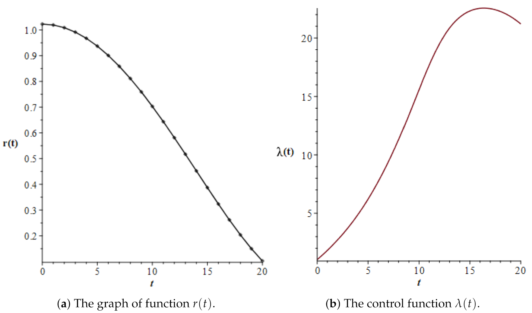
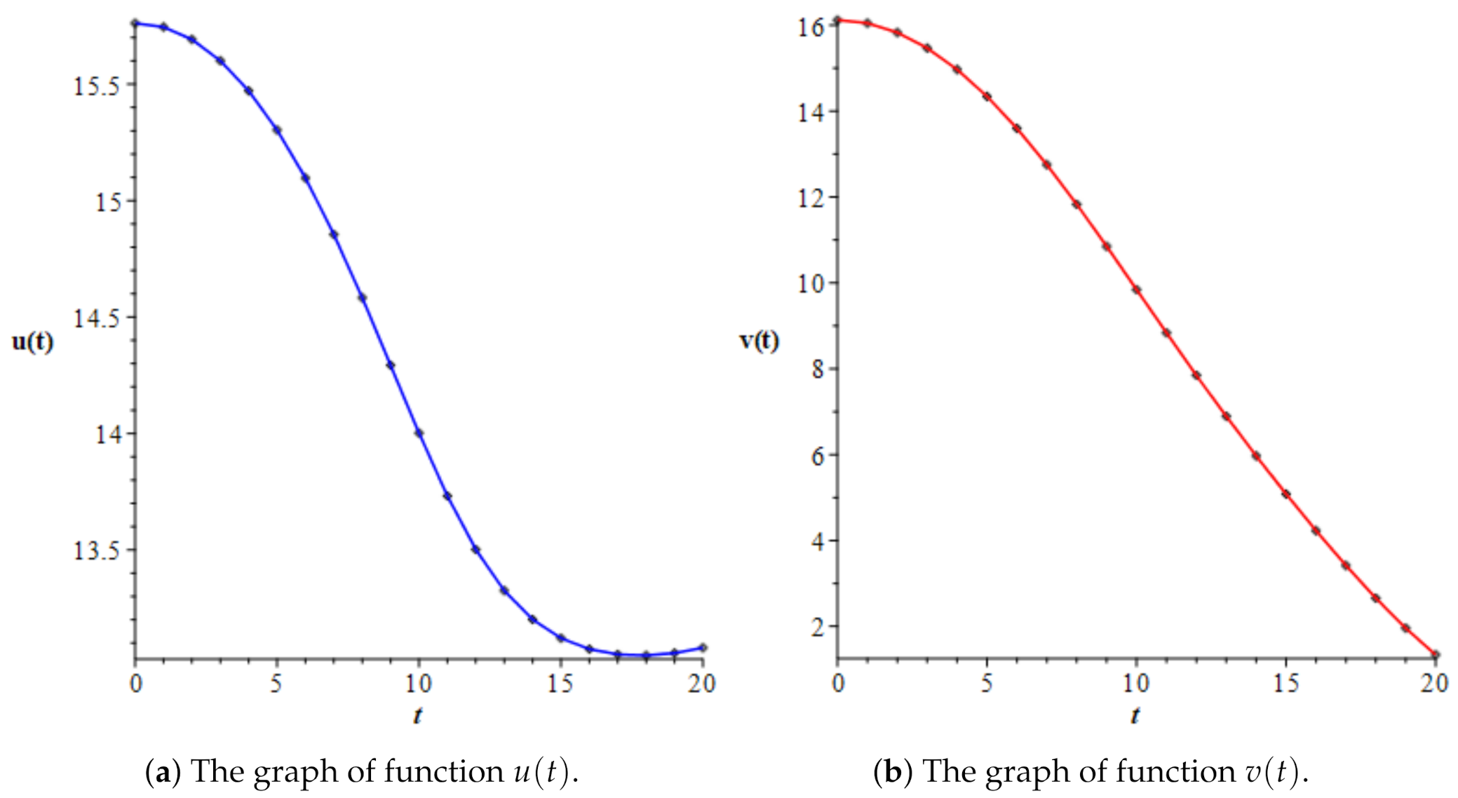
3.3. Numerical Simulations

Below, we illustrate the theoretical results obtained for the first controllability problem by numerical simulations using the Maple software and an modified package for numerical and graphical solutions of Volterra integral equations. The initial Maple package for numerical solutions of Volterra integral equations was published by L.C. Backer and M. Wheeler [29]. For more information about numerical methods for Volterra integral equations, see the books by T.A. Burton [30] and P. Linz [31].
In this section, we compute some numerical simulations considering the system of Volterra integral equations (10); more exactly,
u ( t ) = u 0 c r ( t ) u 0 v 0 r ( t ) c C + 0 t 1 r ( t ) c r ( t ) c C a 1 + b 1 e u ( s ) + b 2 e v ( s ) + c r ( t ) c C A 1 + B e u ( s ) + e v ( s ) d s v ( t ) = v 0 C r ( t ) u 0 v 0 r ( t ) c C + 0 t r ( t ) C r ( t ) c C a 1 + b 1 e u ( s ) + b 2 e v ( s ) + 1 + C r ( t ) c C A 1 + B e u ( s ) + e v ( s ) d s .
For these numerical simulations, we may take the expression of the function r ( t ) given by (8).
We restrict our simulations to two cases: Case 1 (the chronic phase of the disease), where the parameters of the nonlinear Volterra integral system have values such that the condition of chronicity ( d < D < d 1 ) holds a = 5 , b 1 = 0.75 × 10 5 , b 2 = 0.38 × 10 5 , c = 0.05 , A = 7 , B = 0.19 × 10 5 , C = 0.2 ; and Case 2 (the accelerated–acute phase of the disease), where the parameters of the nonlinear Volterra integral system have values such that the condition of the accelerated–acute phase ( d 1 < D ) holds a = 5 , b 1 = 0.75 × 10 5 , b 2 = 0.38 × 10 5 , c = 0.05 , A = 7 , B = 0.19 × 10 5 , C = 0.1 . The parameters of the function r ( t ) are k 0 = 0.1 , T = 20 , n = 2 , m = 1 / 2 , T 0 = 0 and the initial conditions for this two simulations are u 0 = 15.76142071 , v 0 = 16.11809565 . The above parameter values were first estimated in the paper of Dingli and Michor [16], and we have analyzed this set of parameters in our previous work Parajdi et al. [22]. The step size for the numerical integration is h = 0.1 .
Note that, although no longer relevant to clinical practice, in order to illustrate how the overall appearance of λ ( t ) changes with different model parameters, we have made computations for a parameter set of chronic myeloid leukemia (CML) as well. This describes a purely hypothetical case in which a chronic disease was treated with conventional chemotherapy (for the chronic phase of CML see Figure 1 and Figure 2, and Table 1, and in addition for the accelerated-acute phase of CML see Figure 3 and Figure 4, and Table 2).

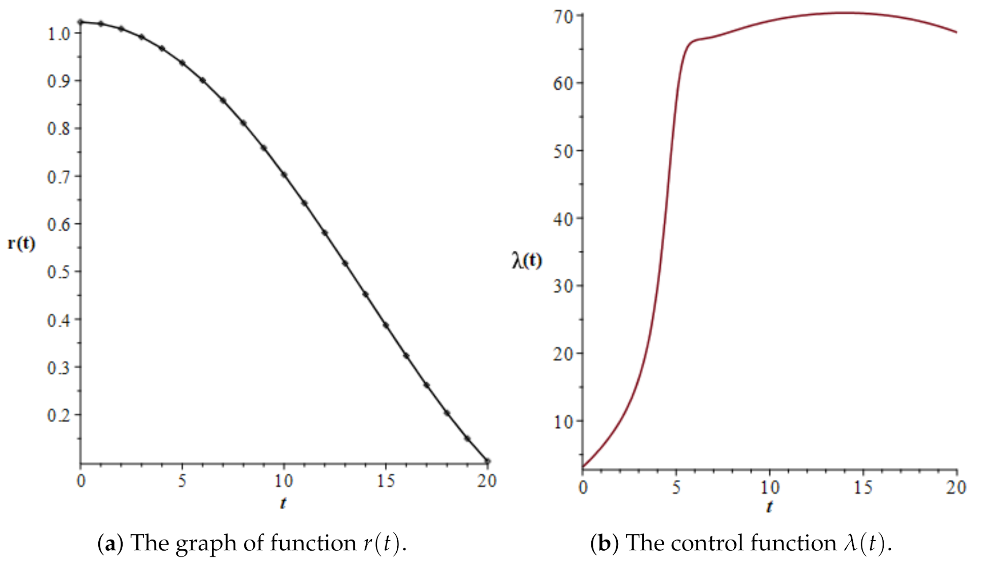
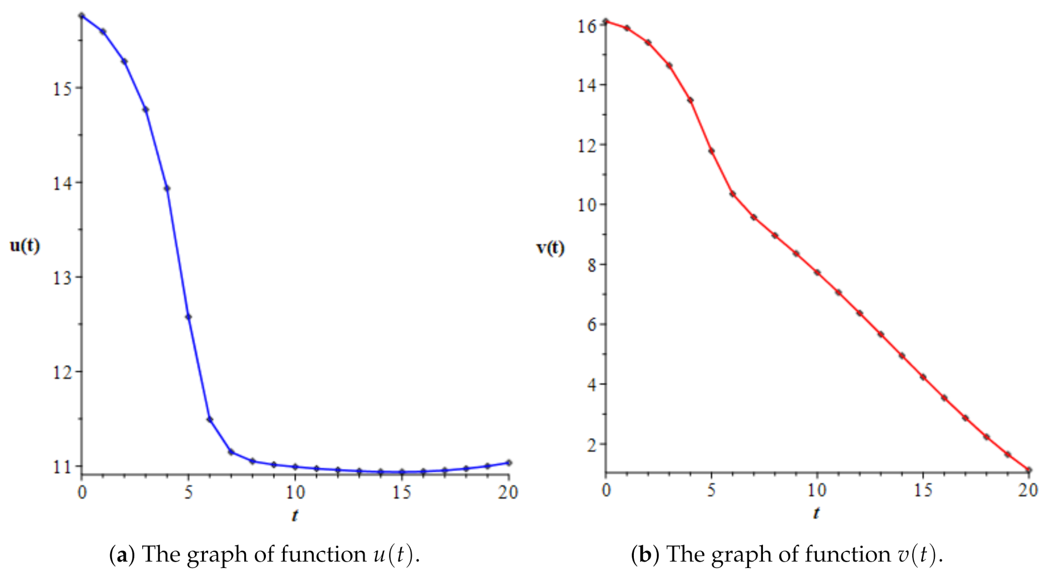
3.4. A Different Objective Condition

As already noted, some other objective conditions can be considered for the first control problem. One of these, with immediate practical importance, consists of following a predefined path for the ratio y t / x t instead of ln y t / ln x t from (7). Hence, given a function r t with k 0 y 0 x 0 r t y 0 x 0 t 0 , T , r 0 = y 0 / x 0 and r T = k 0 y 0 / x 0 , we look for λ t such that problem (4) has a solution x , y such that
y t x t = r t , t 0 , T .
With the notations from Section 3.1, from (5), one has
v t u t = v 0 u 0 + 0 t A 1 + B e u + e v a 1 + b 1 e u + b 2 e v d s + c C 0 t λ s d s .
Assuming that C c and taking into account that v t u t = ln y t / x t , we find
0 t λ s d s = 1 c C ln r t ln r 0 + 0 t a 1 + b 1 e u + b 2 e v A 1 + B e u + e v d s .
Hence,
λ t = 1 c C r t r t + a 1 + b 1 x t + b 2 y t A 1 + B x t + y t .
This gives the expression of F ˜ x , y , and adding this into the integral equivalent version of (4) leads to a fixed point equation in x , y which, as in Section 3.1, has a unique solution.
The stability of the solution and numerical simulations for this problem can be determined similarly.

4. Second Control Problem for the Normal–Leukemic System

Our second problem for the normal–leukemic cell dynamic system is to reduce the leukemic cell population to an acceptable level; this time, by controlling the proliferation rate of leukemic cells. Thus, we consider the system
x = a x 1 + b 1 x + b 2 y c x y = λ A y 1 + B x + y C y x 0 = x 0 , y 0 = y 0
where number λ > 0 is the control parameter.

4.1. Solving of the Control Problem

Making the same change of variables as above yields the following system of integral equations:
u t = u 0 c t + 0 t a 1 + b 1 e u + b 2 e v d s v t = v 0 C t + λ 0 t A 1 + B e u + e v d s
to which we associate the objective condition
v T = v T ,
where v T is the expected level of leukemic cells after a period of time T .
Compared with the abstract problem from Section 2, here
W = C 0 , T , R 2 , Λ = R + , D = { u , v , λ C 0 , T , R 2 × R + : v T = v T }
and system (14) stands for the fixed point equation w = N w , λ , with w = u , v .
Applying the general principle given by Proposition 1, we obtain the following controllability result.
Theorem 3.
For each number v T with max 0 , v 0 C T < v T < v 0 , the control problem (14) and (15) has a solution u , v , λ C 0 , T , R 2 × 0 , + .
Proof. 
Let u , v Σ 1 , that is u , v C 0 , T , R 2 solves (14) for some λ R + . From the second equation of (14), we then have
λ = 1 0 T A 1 + B ( e u + e v ) d s v T v 0 + C T ,
hence, F : Σ 1 R + is given by
F u , v = 1 0 T A 1 + B ( e u + e v ) d s v T v 0 + C T .
Clearly, we may extend F from Σ 1 to C 0 , T , R 2 by using the same expression, namely
F ˜ u , v = 1 0 T A 1 + B ( e u + e v ) d s v T v 0 + C T for u , v C 0 , T , R 2 .
Now, our fixed point equation w = N ˜ w , with N ˜ w = N w , F ˜ w , becomes
u = u 0 c t + 0 t a 1 + b 1 e u + b 2 e v d s v = v 0 C t + v T v 0 + C T 0 T A 1 + B ( e u + e v ) d s 0 t A 1 + B e u + e v d s .
Hence,
N ˜ 1 u , v t = u 0 c t + 0 t a 1 + b 1 e u + b 2 e v d s , N ˜ 2 u , v t = v 0 C t + v T v 0 + C T 0 T A 1 + B ( e u + e v ) d s 0 t A 1 + B e u + e v d s .
The existence of a fixed point w of N ˜ can be guaranteed by using Schauder’s fixed point theorem. Indeed, the operator N ˜ is completely continuous, as follows immediately from the Arzelà–Ascoli theorem. On the other hand, one has
u 0 c T N ˜ 1 u , v t u 0 + a T , v 0 C T N ˜ 2 u , v t v T + C T .
Consequently, there are R 1 , R 2 > 0 with
N ˜ 1 u , v R 1 , N ˜ 2 u , v R 2
for all u , v C 0 , T . Hence, N ˜ S S , where S : = { u , v C 0 , T , R 2 : u R 1 , v R 2 } . Thus, Schauder’s fixed point theorem applies and guarantees the existence in S of a fixed point w = u , v of N ˜ . Finally, the control λ is calculated using Formula (16), with u and v thus determined. □
Remark 3.
Since (13) is a Volterra system with Lipschitz nonlinearities, for any given λ , system (13) has a unique solution u , v . In particular, for the value λ corresponding to a solution u , v , λ of the control problem, the trajectory u , v is unique. We may interpret this note in the following way: for a prescribed drug dose, the patient’s evolution is uniquely determined.

4.2. Stability of the Control Problem

Theorem 4.
Let u , v , λ be a solution of the control problem (14) and (15). For a given λ ¯ R + , denote by u ¯ , v ¯ the corresponding solution of system (14) and v ¯ T : = v ¯ T . Then, for any small ε > 0 , one has
λ ¯ λ ε A T e a + λ A T = : δ implies v ¯ T v T ε .
Proof. 
As before, using the Lipschitz estimates, one has
u t u ¯ t a 0 t u s u ¯ s + v t v ¯ t d s ,
v t v ¯ t λ λ ¯ 0 t A 1 + B e u ¯ + e v ¯ d s + λ 0 t A 1 + B e u ¯ + e v ¯ A 1 + B e u + e v d s A T δ + λ A 0 t u u ¯ + v v ¯ d s .
Then, taking the sum
u t u ¯ t + v t v ¯ t a + λ A 0 t u s u ¯ s + v t v ¯ t d s + A T δ
and Gronwall’s inequality yields
u t u ¯ t + v t v ¯ t A T δ e a + λ A t .
In view of the expression of δ , this implies
v ¯ T v T ε .
Remark 4.
Estimate (18) shows us that for a treatment λ ¯ close enough to the prescribed treatment λ , the patient’s evolution u ¯ t , v ¯ t remains in the vicinity of the prescribed evolution u t , v t .

5. Discussion

Model applicability: In the developmental hierarchy of bone marrow, whether normal or leukemic, there are four cell types (stem cells, progenitors, differentiated, and terminally differentiated). Our model aggregates over the properties of all cell types in the hierarchy to model a unique cell type for the normal phenotype and another unique cell type for the leukemic phenotype. Our abstract cells have regulatory negative feedback on the growth found at the stem cell level 1 / ( 1 + b 1 x + b 2 y ) and 1 / 1 + B x + B y , respectively), the high growth rates of progenitor cells (large a and A), and the differentiated and terminally differentiated bulk mass effect, which eventually accounts for the disease dynamics.
Although our model was developed for chronic myelogenous leukemia, it applies to any leukemia type, acute or chronic, as long as it can be assumed that, over the considered timespan, all basic parameters of cell kinetics are time invariant. It does not apply to the natural course of chronic leukemia as a whole, from subclinical to blast crises, where the growth rate A increases by orders of magnitude with disease progression.
Moreover, our model can be easily extended to other physiological conditions. In our stability analysis, we have defined the satisfactory success criterion as r ¯ r < ε , allowing for small deviances both above and beyond the set point. This relates our model to general models of tissue development and homeostasis, where two normal cell populations (instead of normal and leukemic) compete for space but are both desirable and are regulated by a single molecular signal (instead of chemotherapy).
First control problem: We divided up the treatment protocol into two phases. The first is a burn-in phase, from time t = 0 to T 0 , in which the drug infusion only freezes the cellular status quo, keeping the malignant/normal cells ratio constant in time (at pretreatment value). In practice, this phase should be very short, as it exposes the patient to additional drug toxicity. It could be useful in clinical trial settings to assess the side effects of chemotherapy separately from the effects of the disease progression or to avoid tumor lysis syndrome at the onset of an induction cycle.
In the next phase, from t = T 0 to final T , the tumor mass is reduced along a predefined curve, with its final point dependent on the subunitary parameter k 0 , and its steepness on the exponent m .
Theorem 2 explores the stability conditions of the control problem, namely establishing the maximum allowable deviation of the drug delivery rate from an ideal delivery schedule, such as if the actual endpoint of the treatment remains within the vicinity of the desired endpoint (only a small fraction of malignant cells remaining, k 0 v 0 / u 0 ). Crucially, we found the admissible error for the infusion function λ t to decrease exponentially with both the growth rates a (of the normal cells) and A (of leukemic cells). This suggests that it may be much harder to achieve an ideal control of acute leukemia, compared to other tumor types, due to the higher division rates of leukemia and its normal cellular background. The admissible error only depends inversely on a linear combination of the cell decay rates c and C , indicating that the rates of spontaneous cell death only marginally influence the control compared with the growth rates.
We found the same inverse exponential dependence on the total time treatment, T . Acute leukemia cannot be equated with a “time-compressed” version of chronic leukemia, which behaves and is treated quite differently. Still, our results may suggest generally that the control of a slowly growing tumor, over a longer time, is equally hard to obtain as the control of an “acute” tumor over a shorter time span, insofar as the assumptions of our model hold.
In practice, the main sources of oscillations of the drug delivery function λ t are the pharmacokinetic excursions of systemic drug levels, since chemotherapy is administered discontinuously. Our results establish a theoretical limit for how large these excursions can be, while still allowing for a cure (and implicitly a limit on the interdose intervals).
Second control problem: We obtained a similar exponential relation for the stability of the second control problem (Theorem 4), where the drug dose lambda is constant in time. The caveat here is that factor is e a + λ A T instead of e a + A T . This implies that, with faster leukemic cell production rates A and a subsequent need for higher drug levels λ , to achieve the same end result, the control is exponentially harder to obtain.

Author Contributions

Conceptualization, R.P.; methodology, L.G.P. and R.P.; software, L.G.P.; validation, I.Ş.H. and L.G.P.; formal analysis, L.G.P. and R.P.; investigation, I.Ş.H., L.G.P. and R.P.; resources, I.Ş.H. and L.G.P.; data curation, I.Ş.H. and L.G.P.; writing-original draft preparation, L.G.P. and R.P.; writing-review and editing, L.G.P. and R.P.; visualization, L.G.P.; supervision, I.Ş.H. All authors have read and agreed to the published version of the manuscript.

Funding

This research received no external funding.

Institutional Review Board Statement

Not applicable.

Informed Consent Statement

Not applicable.

Data Availability Statement

Not applicable.

Acknowledgments

Authors are thankful to the reviewers for their useful comments and constructive remarks that helped to improve the presentation of the paper.

Conflicts of Interest

The authors declare no conflict of interest.

References

  1. DeVita, V.T., Jr.; Chu, E. A History of cancer chemotherapy. Cancer Res. 2008, 68, 8643–8653. [Google Scholar] [CrossRef] [PubMed] [Green Version]
  2. Steensma, D.P.; Kyle, R.A. Hematopoietic stem cell discoverers. Mayo Clin. Proc. 2021, 96, 830–831. [Google Scholar] [CrossRef] [PubMed]
  3. Bonnet, D. Leukemic stem cells show the way. Folia Histochem. Cytobiol. 2005, 43, 183–186. [Google Scholar] [PubMed]
  4. Schättler, H.; Ledzewicz, U. Optimal Control for Mathematical Models of Cancer Therapies: An Application of Geometric Methods; Springer: New York, NY, USA, 2015. [Google Scholar]
  5. Friberg, L.E.; Henningsson, A.; Maas, H.; Nguyen, L.; Karlsson, M.O. Model of chemotherapy-induced myelosuppression with parameter consistency across drugs. J. Clin. Oncol. 2002, 20, 4713–4721. [Google Scholar] [CrossRef]
  6. Arimoto, M.K.; Nakamoto, Y.; Nakatani, K.; Ishimori, T.; Yamashita, K.; Takaori-Kondo, A.; Togashi, K. Increased bone marrow uptake of 18F-FDG in leukemia patients: Preliminary findings. SpringerPlus 2015, 4, 521. [Google Scholar] [CrossRef] [Green Version]
  7. Ohanian, M.; Faderl, S.; Ravandi, F.; Pemmaraju, N.; Garcia-Manero, G.; Cortes, J.; Estrov, Z. Is acute myeloid leukemia a liquid tumor? Int. J. Cancer 2013, 133, 534. [Google Scholar] [CrossRef]
  8. Weaver, B.A. How Taxol/Paclitaxel kills cancer cells. Mol. Biol. Cell 2014, 25, 2677–2681. [Google Scholar] [CrossRef]
  9. Engelhardt, D.; Michor, F. A quantitative paradigm for decision-making in precision oncology. Trends Cancer 2021, 7, 293–300. [Google Scholar] [CrossRef]
  10. Afenya, E.K. Using mathematical modeling as a resource in clinical trials. Math. Biosci. Eng. 2005, 3, 421–436. [Google Scholar] [CrossRef]
  11. Afenya, E.K.; Bentil, D.E. Some perspectives on modeling leukemia. Math. Biosci. 1998, 150, 113–130. [Google Scholar] [CrossRef]
  12. Berezansky, L.; Bunimovich-Mendrazitsky, S.; Shklyar, B. Stability and controllability issues in mathematical modeling of the intensive treatment of leukemia. J. Optim. Theory Appl. 2015, 167, 326–341. [Google Scholar] [CrossRef]
  13. Bratus, A.S.; Fimmel, E.; Todorov, Y.; Semenov, Y.S.; Nuernberg, F. On strategies on a mathematical model for leukemia therapy. Nonlinear Anal. Real World Appl. 2012, 13, 1044–1059. [Google Scholar] [CrossRef]
  14. Crowell, H.L.; MacLean, A.L.; Stumpf, M.P.H. Feedback mechanisms control coexistence in a stem cell model of acute myeloid leukaemia. J. Theor. Biol. 2016, 401, 43–53. [Google Scholar] [CrossRef] [Green Version]
  15. Cucuianu, A.; Precup, R. A hypothetical-mathematical model of acute myeloid leukaemia pathogenesis. Comput. Math. Methods Med. 2010, 11, 49–65. [Google Scholar] [CrossRef]
  16. Dingli, D.; Michor, F. Successful therapy must eradicate cancer stem cells. Stem. Cells 2006, 24, 2603–2610. [Google Scholar] [CrossRef] [Green Version]
  17. Djulbegovic, B.; Svetina, S. Mathematical model of acute myeloblastic leukaemia: An investigation of the relevant kinetic parameters. Cell Prolif. 1985, 18, 307–319. [Google Scholar] [CrossRef]
  18. Foley, C.; Mackey, M.C. Dynamic hematological disease: A review. J. Math. Biol. 2009, 58, 285–322. [Google Scholar] [CrossRef]
  19. Kim, P.S.; Lee, P.P.; Levy, D. Modeling regulation mechanisms in the immune system. J. Theor. Biol. 2007, 246, 33–69. [Google Scholar] [CrossRef]
  20. Mac Lean, A.L.; Lo Celso, C.; Stumpf, M.P.H. Population dynamics of normal and leukaemia stem cells in the haematopoietic stem cell niche show distinct regimes where leukaemia will be controlled. J. R. Soc. Interface 2013, 10, 20120968. [Google Scholar] [CrossRef] [Green Version]
  21. Moore, H.; Li, N.K. A mathematical model for chronic myelogenous leukemia (CML) and T cell interaction. J. Theor. Biol. 2004, 227, 513–523. [Google Scholar] [CrossRef]
  22. Parajdi, L.G.; Precup, R.; Bonci, E.A.; Tomuleasa, C. A mathematical model of the transition from normal hematopoiesis to the chronic and accelerated-acute stages in myeloid leukemia. Mathematics 2020, 8, 376. [Google Scholar] [CrossRef] [Green Version]
  23. Precup, R. Mathematical understanding of the autologous stem cell transplantation. Ann. Tiberiu Popoviciu Semin. Funct. Equ. Approx. Convexity 2012, 10, 155–167. [Google Scholar]
  24. Precup, R.; Serban, M.A.; Trif, D.; Cucuianu, A. A planning algorithm for correction therapies after allogeneic stem cell transplantation. J. Math. Model. Algorithms 2012, 11, 309–323. [Google Scholar] [CrossRef]
  25. Rubinow, S.I.; Lebowitz, J.L. A mathematical model of the acute myeloblastic leukemic state in man. Biophys. J. 1976, 16, 897–910. [Google Scholar] [CrossRef] [Green Version]
  26. Sharp, J.A.; Browning, A.P.; Mapder, T.; Baker, C.M.; Burrage, K.; Simpson, M.J. Designing combination therapies using multiple optimal controls. J. Theor. Biol. 2020, 497, 110277. [Google Scholar] [CrossRef]
  27. Mackey, M.C.; Glass, L. Oscillation and chaos in physiological control systems. Science 1977, 197, 287–289. [Google Scholar] [CrossRef]
  28. Barbu, V. Mathematical Methods in Optimization of Differential Systems; Springer Science+Business Media: Dordrecht, The Netherlands, 1994. [Google Scholar]
  29. Becker, L.C.; Wheeler, M. Numerical and Graphical Solutions of Volterra Equations of the Second Kind; Maple Application Center: Waterloo, ON, Canada, 2005. [Google Scholar]
  30. Burton, T.A. Volterra Integral and Differential Equations, 2nd ed.; Mathematics in Science & Engineering; Elsevier: Amsterdam, The Netherlands, 2005; Volume 202. [Google Scholar]
  31. Linz, P. Analytical and Numerical Methods for Volterra Equations; Studies in Applied Mathematics; SIAM: Philadelphia, PA, USA, 1985; Volume 7. [Google Scholar]
Figure 1. The graph of the function r ( t ) and the graph of the control function λ ( t ) in Case 1 (chronic phase) of the simulations.
Symmetry 13 01867 g001
Figure 2. The approximate solutions of the system of two nonlinear Volterra integral equations, given by (10), obtained in Case 1 (chronic phase).
Symmetry 13 01867 g002
Figure 3. The graph of the function r ( t ) and the graph of the control function λ ( t ) in Case 2 (accelerated–acute phase) of simulations.
Symmetry 13 01867 g003
Figure 4. The approximate solutions of the system of two nonlinear Volterra integral equations, given by (10), obtained in Case 2 (accelerated–acute phase).
Symmetry 13 01867 g004
Table 1. Numerical simulations of the system of two nonlinear Volterra integral equations, given by (10), obtained in Case 1 (the chronic phase of the disease).
tu(t)v(t)v(t)/u(t) λ ( t )
0.015.7614216.118101.022631.03667861
1.015.7455916.046911.019141.82681929
2.015.6921815.828581.008692.72096808
3.015.6009015.466820.991413.73208846
4.015.4714114.967890.967454.88700566
5.015.3032414.340540.937096.21220861
6.015.0967113.596670.900647.72168000
7.014.8544412.752380.858499.42156274
8.014.5827911.828260.8111111.31917081
9.014.2929710.848950.7590413.40181913
10.014.001969.841830.7028915.58459339
11.013.731388.833910.6433417.68482475
12.013.501887.846450.5811419.48688614
13.013.325226.890670.5171220.85563950
14.013.201035.969060.4521721.77786674
15.013.120775.081150.3872622.31403995
16.013.073844.228540.3234322.53852452
17.013.051293.416880.2618022.51022240
18.013.046942.655690.2035522.26679888
19.013.057031.957600.1499321.82786481
20.013.079651.337560.1022621.19948845
Table 2. Numerical simulations of the system of two nonlinear Volterra integral equations, given by (10), obtained in Case 2 (the accelerated–acute phase of the disease).
tu(t)v(t)v(t)/u(t) λ ( t )
0.015.7614216.118101.022633.15804
1.015.5932115.891611.019146.05741
2.015.2779315.410731.008699.93469
3.014.7679514.641030.9914116.19792
4.013.9349213.481410.9674529.76677
5.012.5776811.786440.9370957.07073
6.011.4928010.350850.9006466.27579
7.011.148179.570580.8584966.82106
8.011.050908.963500.8111167.63740
9.011.014128.360170.7590468.47741
10.010.991747.725980.7028969.17105
11.010.973557.059690.6433469.69562
12.010.958246.368250.5811470.06188
13.010.946515.660610.5171270.28064
14.010.939374.946420.4521770.35631
15.010.937704.235730.3872670.28740
16.010.942243.539100.3234370.06809
17.010.953642.867700.2618069.68924
18.010.972482.233440.2035569.13897
19.010.999331.649090.1499368.40266
20.011.034771.128450.1022667.46265
Publisher’s Note: MDPI stays neutral with regard to jurisdictional claims in published maps and institutional affiliations.

