Abstract
Traditionally, the interval and delay effects have been identified and considered as the same anomaly in the context of intertemporal choice, when individuals or groups of individuals make their decisions about reward preferences. This has supposed that most studies on this topic have been focused on the delay effect and, consequently, that the discount functions provided by the existing literature have considered only this effect. This is the case of hyperbolic discounting, which has been used to describe the delay, but not the interval effect. Therefore, the main objective of this paper is to carry out a detailed analysis of both anomalies, which will allow us to mathematically relate them, thus finding their analogies and differences. To do this, we will first analyze the concept of delay effect and later the different definitions of the interval effect. The main conclusion of this paper is twofold. On the one hand, if the benchmark for valuation is fixed, the delay effect coincides with the so-called decreasing interval effect. On the other hand, if the assessment reference point is the beginning of each interval, both anomalies are different. These findings make necessary to redefine the concept of interval effect. Finally, we will analyze the relationship between the interval effect, the delay effect and the subadditivity
1. Introduction
Intertemporal decisions refer to the choice of a reward among a series of alternative actions available at different moments of time so that the made decision is the most profitable for the individual. This is because, continuously, all individuals are immersed in a great dilemma: to obtain less benefit and pay less immediately, or to obtain greater benefits and pay more after a period of time [1,2,3]. Samuelson [4] was one of the first scholars to describe this phenomenon through his discounted utility (DU) model, which has been used up to now as the prominent discount model.
However, from the 1980s onward, a series of counterexamples of the DU model began to emerge in the context of what is currently known as behavioral finance (see, for example, [5,6,7]). This new setting favored a new way of studying finance since, after numerous empirical studies, it was demonstrated that people make irrational decisions [8] in that they do not fit the DU model initially provided by Samuelson [4]. In effect, this model does not explain certain behaviors of the decision maker, known as anomalies or paradoxes in intertemporal choice: the delay effect [9,10], the magnitude effect [9,10,11], speedup–anticipation asymmetry [10,12] and the improving sequence effect [1,13,14,15,16], among others.
Over the last 30 years, attempts have been made to find some mathematical solutions able to cover the deficiencies presented by the DU model. Among them, we can find the hyperbolic discount model [2,17], in which the discount rate decreases with the passage of time, thus solving the anomaly called the delay effect or decreasing impatience, demonstrated for monetary decisions [9,10] and non-monetary decisions [18,19].
Later, some scholars detected that the delay effect was sometimes identified with another paradox: the so-called interval effect [20]. This confusion has resulted in very little research on this anomaly. In effect, most proposed functions aim to solve the delay effect, but few of them characterize the interval effect [21,22]. As a result, Read [23], when describing the interval effect, points out that “A systematic analysis of the relative contributions of delay and interval to discounting is yet to be done”. Therefore, the objective of this paper is to analyze the concept of the interval effect and analyze the similarities and differences between this anomaly and the delay effect. Moreover, we will study the relationship between both effects and the concept of subadditivity [24,25].
Some of these anomalies have been widely analyzed in different fields of research, such as psychology, medicine, finance, economics, marketing and even in business decisions. However, this has not been analysis on the case of the interval effect, which has begun to be studied in medicine and finance but has hardly been developed in other disciplines. That is why this paper intends to change this trend and open a new field of research in managerial decision-making.
If the interval effect means that the discount rate tends to be higher the closer the reward is to its equivalent amount [26], we could extrapolate this definition to managerial decisions in order to choose between three investment strategies (A, B and C) of a company, whose profits will be obtained in the short, medium and long term, respectively (assume that the short, medium and long term are equidistant from each other, e.g., 6, 12 and 18 months). In the beginning, a rational manager (constant discount rate) could be indifferent to the choice of any of the three former strategies. However, if the interval effect is present in managerial decisions, according to its definition, the manager could prefer to implement strategy A over strategy B and could prefer strategy B over strategy C (he prefers the closest option in small intervals). Nevertheless, by using the definition provided by Read [20] and Scholten and Read [26], the manager would choose strategy C over strategy A (he chooses the latest option for wider intervals). Observe that this leads to a contradiction in his decision-making; that is to say, it leads to an inconsistency.
The study of the interval effect, as well as the delay effect in making decisions, can help to understand the behavior of managers and to answer some questions such as the following: Is there an interval effect or a delay effect in managerial decisions? Are there any differences in short- and long-term managerial decision-making between small businesses and large companies? Is the net present value (NPV) based on Samuelson’s exponential discount [4] a good tool for business decision-makers? The answers to these questions and many others can help to open a wide field of research in the strategic direction of a company.
This paper is structured as follows. In Section 2, we will define the concept of the delay effect while, in Section 3, we will focus on clarifying the concept of the interval effect. Section 4 will provide the joint mathematical analysis of the interval and delay effects. Finally, Section 5 summarizes and concludes the paper.
2. The Delay Effect
The delay effect, or common difference effect, means that the discount rate decreases as the delay increases; that is to say, the discount rate is lower for intervals of the same length starting later. This effect is one of the most studied anomalies. The first authors, who analyzed this effect, were Prelec and Loewenstein [12]. Let us see an example to explain this concept [22].
Example 1.
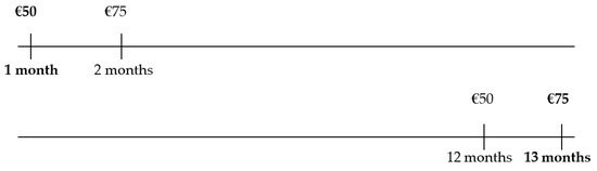
A person may prefer receiving EUR 50 in a month to EUR 75 in two months. However, this same person may prefer EUR 75 within 13 months to EUR 50 within 12 months. Observe that, between the two rewards, there is a difference of one month (from 1 to 2 and from 12 to 13). However, the preferences of the decision-maker have changed, resulting in a time inconsistency which is not compatible with the exponential discount function, since we have gone from preferring the EUR 50 reward in a month to preferring the EUR 75 reward in the thirteenth month (in both cases, there was an increase of the delay in 11 months). See Figure 1.
Figure 1.
Delay effect (Example 1) (in bold, the chosen option). Source: Own elaboration.
This would be equivalent to an Example 2 beginning with the following statement:
Example 2.
A person may be indifferent between receiving EUR 50 in a month and receiving EUR 75 in two months. However, this same person may prefer EUR 75 within 13 months to EUR 50 within 12 months.
Therefore, mathematically, this effect can be formalized as follows:
where x and y () represent the rewards equivalent at instants s and t, respectively, and denotes the incremental delay (in Examples 1 and 2, ε is 11 months) applied to each reward. Specifically, the mathematical expression of the immediacy effect is a particular case of the delay effect and would remain in the following form [27]:
where x and y () represent the rewards equivalent at instants and t, respectively, and denotes the incremental delay.
3. The Interval Effect
The interval effect, also called the interval length effect, was demonstrated by Read [20]. This scholar distinguished between the delay and interval effects, thus opening a new field of research between two anomalies which, traditionally, have been studied as only one, namely the delay effect. Read [20] stated that the discount rate depends on the length of the interval in such a way that the larger the interval, the smaller the discount rate.
Later, Read and Roelofsma [28] identified the interval effect with subadditive discounting (“for a given delay, the total discounting is greater when it is broken into intervals, and discounting measured separately for each interval, than when it is left unbroken”) and Read [23] completed the definition of the interval effect as “shorter intervals lead to more discounting per-time-unit”.
The following works based their definitions on previous studies. Thus, Scholten and Read [26] provided another definition of this effect: “the discount rate will tend to be higher the closer the rewards are to each other”. On the other hand, Kinari et al. [29] stated that the interval effect is a more general concept than subadditive time discounting; that is, the longer the interval, the lower the per period time discount rate. Moreover, the delay effect leads to an examination of the interval effect as a by-product.
As indicated in the former definitions, there is unanimity in that the interval effect means that the larger the interval, the smaller the discount rate. However, Read [20] and Read and Roelofsma [28] identified this concept with that of subadditivity, and later, Kinari et al. [29] stated that the interval effect is a more general concept than subadditivity time discounting, in the same way that it regards the interval effect as a by-product of the delay effect. However, none of these statements have been mathematically shown, as there is not a mathematical concept of the interval effect or of the different situations in which this anomaly can appear. Later, Cruz Rambaud and Ortiz Fernández [22] mathematically demonstrated that, from a dynamic point of view, it can be deduced that subadditivity is a particular case of the delay effect. Therefore, the relationship between the interval effect, the delay effect and subadditivity remains to be demonstrated. Table A1 (see Appendix A) summarizes the characteristics of the papers analyzing the interval effect.
Next, we are going to analyze the mathematical concept of the interval effect, as well as the possible situations in which it can occur. First, let us see an example (Figure 2).
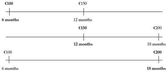
Figure 2.
Interval effect. (The chosen option is in bold. Source: Own elaboration.
Example 3.
A subject faces three intertemporal choices: the first two will be separated by intervals of the same length, and the length of the third interval is the sum of the lengths of the former intervals.
Under the interval effect, a decision-maker could prefer EUR 100 to EUR 150 and, moreover, he or she could prefer EUR 150 over EUR 200. Both choices are separated by a time horizon of 6 months or, in other words, they are separated by an interval of a length equal to 6 months. However, we can find a third intertemporal choice, in which the decision-maker must choose between EUR 100 within 6 months and EUR 200 12 months later (that is, in 18 months). In this case, the decision-maker could opt to choose EUR 200 and wait for 12 months more. As indicated, in the 6 month intervals, the decision-maker could prefer the earliest option while, in the 12 month interval, the decision-maker could prefer to wait. It can be observed that, for the smallest interval, the earliest option is chosen, and for the largest interval, the latest option is preferred, giving rise, as in Example 1, to time inconsistency.
Mathematically, this effect can be formalized as follows [29]:
where .
Example 3 is based on quantities, but what about the discount rates? Observe that, in the 6 month intervals, the discount rates are greater than in the 12 month interval. From a theoretical point of view, we can write this as follows:
and
where is he discount rate in the interval , the discount rate in the interval and the discount rate in the interval (). Definitively, joining the two former inequalities into one yields
As stated in [21], the discount rate depends on the length of the interval in such a way that the larger the interval, the smaller the discount rate. On the other hand, we can introduce the following definition.
Definition 1.
Given a stationary (resp., dynamic) discount function, the average discount ratio associated with the interval(resp.,), denoted by(resp.,), is defined as the geometric mean of the corresponding discount ratio(resp.,), which is to say that
(resp.,), where a and b are non-negative real numbers.
The following proposition gives two basic properties of the average discount ratio for the stationary case (the statements for the dynamic case are analogous).
Proposition 1.
The following equalities hold:
- 1.
- , whereis the mean discount rate in the interval;
- 2.
- , whereis the instantaneous discount rate at time t.
Proof.
In effect, the following can be said:
- The general expression of a discount function, according to its instantaneous discount rate, leads to and Therefore, as is the average of function in the interval , one haswhich is the required equality;
- , which is an indetermination. Let us solve this indetermination by using the well-known formula to solve this type of indetermination:
□
4. Mathematical Analysis of the Delay and Interval Effects
As formerly indicated, the delay and interval effects are different in spite of the fact that, in some specific cases, they coincide. This is the reason why they have been traditionally confused. In effect, the difference between them is based on the difference between time as a delay and time as an interval.
In Figure 3, we can see that the interval a is the difference between the delays s and t, which is to say that
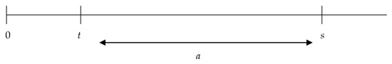
Figure 3.
Time as a delay and time as an interval. Source: Own elaboration.
This can also be expressed as
In a beginning, Table 1 clarifies the difference between both concepts.

Table 1.
Differences between the delay and interval effects. Source: Own elaboration.
However, the definition of the interval effect provided by Kinari et al. [29,30] does not consider the restriction of equal delays of the intervals involved in the definition. For this reason, we are going to analyze all possible situations with different intervals independently of the delays associated with the intervals involved in the analysis. These scholars even consider that the interval effect is a particular case of the delay effect. In effect, the following subsections demonstrate that the delay effect can be derived as a particular case of the interval effect. Table 2 summarizes the definitions of the interval effect analyzed in this paper.
Table 2.
Some definitions of the interval effect. Source: Own elaboration.
The definitions by Read [4] and Read and Roelofsma [28] state that shorter intervals will exhibit greater discount rates; that is to say, the longer interval, the lower the per period time discount rate, which corresponds to the definitions by Kinari et al. [29,30], stating that the per period time discount rate decreases as the interval lengthens.
4.1. Assessment at a Given Benchmark (Time 0)
Let s denote the left endpoint of the shorter interval (of length a), and let t denote the left endpoint of the larger interval (of length b). Therefore, . If, moreover, , then we can provide the following definition.
Definition 2.
A stationary discount function is said to be subadditive of the second order if, for every, it satisfies the following inequality [27]:
Specifically, if , then
which is subadditivity. If F is differentiable, the following theorem holds.
Theorem 1.
The following conditions are equivalent:
- (i)
- If, then;
- (ii)
- The instantaneous discount rate is strictly decreasing;
- (iii)
- If, then;
- (iv)
- The delay effect holds;
- (v)
- The subadditivity of the second order holds.
Proof.
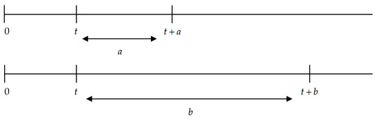
(i) ⇒ (ii). Assume that, if , then . In this case, the intervals exhibit equal left endpoints and different lengths () (see Figure 4). □
Figure 4.
Condition (1) of Theorem 1. Source: Own elaboration.
In effect, assume that there exist r and s and r < s, such that . If , by continuity, there exists a neighborhood of r, , and a neighborhood of s, , with , such that for every and every , the inequality holds. If we now consider the intervals and , it is easy to verify that and, consequently, , in contradiction with the hypothesis. On the other hand, if , we could consider two cases:
- The instantaneous discount rate is constant in the interval . This is not possible because by taking and , one has , in contradiction with (i);
- The instantaneous discount rate is not constant in the interval . In this case, there is a subinterval of , where the instantaneous discount rate is increasing and, as such, the reasoning is the same as the case in which .
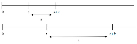
Figure 5.
Condition (iii) of Theorem 1 (I). Source: Own elaboration.
Figure 6.
Condition (iii) of Theorem 1 (II). Source: Own elaboration.
(iii) ⇒ (iv). This is obviously letting and in the inequality , which leads to . However, the case is not possible (see the last paragraphs of the implication (i) ⇒ (ii)).
(iv) ⇒ (v). Assume that and (which implies and ). By the delay effect, one has
or, equivalently,
which is subadditivity of the second order.
(v) ⇒ (i). Assume that . In the definition of subadditivity of the second order, take and . Therefore, in this case, one has
or, equivalently,
Taking Napierian logarithms in both sides of the former inequality, dividing by ε and letting , one has
If , as the former inequality is valid for every a and c, the instantaneous discount rate would be constant in the interval . However, this is not possible, as there would be two amounts m and n such that
where . Observe that (1) follows immediately. This completes the proof.
Corollary 1.
The delay effect implies subadditivity.
Proof.
This is an immediate consequence of Theorem 1, as subadditivity of the second order implies subadditivity (see the remark after Definition 2). □
Analogously, we can enunciate the following theorem. Before we do, we need the following definition.
Definition 3.
A stationary discount function is said to be superadditive of the second order if, for every, it satisfies the following inequality [21]:
Specifically, if , then
which is superadditivity.
Theorem 2.
The following conditions are equivalent:
- (i)
- If, then;
- (ii)
- The instantaneous discount rate is strictly increasing;
- (iii)
- If, then;
- (iv)
- The reverse delay effect holds;
- (v)
- The superadditivity of the second order holds.
Corollary 2.
The reverse delay effect implies superadditivity.
Proof.
This is an immediate consequence of Theorem 2, as superadditivity of the second order implies superadditivity (see the remark after Definition 3). □
Figure 7.
Condition (i) of Theorem 2. Source: Own elaboration.
Figure 8.
Condition (iii) of Theorem 2 (I). Source: Own elaboration.
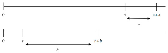
Figure 9.
Condition (iii) of Theorem 2 (II). Source: Own elaboration.
To summarize, in the cases displayed in Figure 5 and Figure 6, the instantaneous discount rate is decreasing, while in the cases displayed in Figure 7, Figure 8 and Figure 9, the instantaneous discount rate is increasing. Finally, the case shown by Figure 10 ( and ) is not mathematically possible.
Figure 10.
Case in which and . Source: Own elaboration.
In effect, by letting by Theorem 1, the instantaneous discount rate has to be decreasing, while by letting by Theorem 2, the instantaneous discount rate has to be increasing. However, both situations are not simultaneously possible. This allows us to conclude that, in the cases in which the short interval begins before or at the same time as the larger interval, the instantaneous discount rate is decreasing and, contrarily, in all cases in which the short interval ends after the larger interval, the instantaneous discount rate is increasing. Obviously, both results are not consistent, and then we have to redefine the interval effect in this context.
In effect, the previous analysis allows us to claim that the former analyzed cases could be descriptive of the so-called interval effect, regardless of whether the discount rate increases or decreases. However, it is necessary to make a distinction, as a given discount function cannot simultaneously fit both situations. Therefore, the interval effect could be classified as follows:
Figure 11 clarifies the involved implications.
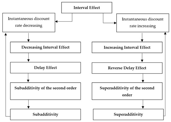
Figure 11.
The interval effect. Source: Own elaboration.
Once the concept of the interval effect has been clarified, another question arises: is the interval effect a by-product of the delay effect? This statement was introduced by Kinari et al. [29,30]. The delay effect depends on the FED of the intervals considered in the analysis, whereas the interval effect depends on length of the involved intervals. However, from a stationary point of view, when the length of the intervals is the same (Figure 1), it can be stated that the delay effect is a by-product (a particular case) of the interval effect, specifically of the decreasing interval effect. This conclusion runs contrary to that stated by Kinari et al. [29,30].
4.2. Assesment at Variable Reference (at the Front-End Delay of the Interval)
In Section 4.1, we measured the instantaneous discount rates with reference to a given benchmark (labeled as time 0). However, the use of discount ratios implies that the process of intertemporal choice is transitive, and there is nothing further from the truth. In effect, the additive property of discount ratios
is not possible because, by the interval effect, the average instantaneous discount rate in the intervals and is greater than the corresponding mean in the interval .
Therefore, we are going to measure the average instantaneous discount rate by using the discount function referenced at the front-end delay of the involved interval. However, it is necessary to take into account that the interval effect obviously implies that, for every s, t and a, the following equality holds:
That is to say, the discount function is stationary. In other words, the analysis of the interval effect with dynamic discount functions does not make sense. If the instantaneous discount rate is decreasing, it is immediate, showing that both the delay and the interval effect hold. However, our aim is to analyze if the interval effect is independent of the delay effect. To do this, we are going to consider the discount function whose instantaneous discount rate is
Integration by parts leads to the following equality:
Moreover, the derivative of is
This means that the average discount rate is lower for larger intervals. Moreover, as the discount function is stationary, the delay effect does not hold.
5. Conclusions and Future Research
In this paper, we clarified the concept of the interval effect which, traditionally, has been confused with the delay effect. The interval effect means that the discount rate is greater the shorter the interval, while the delay effect means that the discount rate is greater the shorter the delay. However, before jointly analyzing these two effects, it was necessary to study the possible cases in which the interval effect can appear. This analysis has allowed for redefining the concept of the interval effect by subdividing it into two sub-concepts:
- The decreasing interval effect, wherein the discount rate decreases (the FED of the short interval is less than or equal to the FED of the larger interval);
- The increasing interval effect, wherein the discount rate increases (the FED of the larger interval is less than the FED of the shorter interval).
From this distinction, we have been able to deduce that, from a stationary point of view, the delay effect and, therefore, the subadditivity are a particular case of the decreasing interval effect under certain conditions, and the reverse implications cannot be stated. In the same way, it has been found that, starting from the increasing interval effect, it is possible to deduce the concept of the reverse delay effect and, therefore, superadditivity.
Another contribution of this paper is that the interval effect does not make sense from a dynamic point of view, since this effect implies a stationary discount function for this effect to exist. Moreover, the interval and delay effects have shown to be independent of each other.
The classical methods included in the paper, such as discount functions, could be extended to include memory effects. In effect, it has been shown that fractional operators with memory modify the delay in biological and other systems, and that could be used to calculate adequate fractional discounts. In this way, [32] introduced the relationship between human decision-making, fractional memory and delays. On the other hand, given the parallelism between discount and probability functions [33], some distributions modeling the delay in human decisions could inspire new discount functions in the ambit of intertemporal choice. In this way, [34] showed that human decision delays present a gamma probability distribution, which can be used to adjust the discount factors weighting the value of different delays. These ideas are proposed as future research.
Finally, another further research line is to analyze the consequences of the delay effect and the interval effect in the field of managerial decision-making.
Author Contributions
The individual contribution of each author has been as follows: writing, methodology, formal analysis and funding acquisition, S.C.R.; writing, conceptualization and supervision, P.O.F. All authors have read and agreed to the published version of the manuscript.
Funding
This research has been funded by the Spanish Ministry of Economy and Competitiveness, grant number DER2016-76053R.
Institutional Review Board Statement
Not applicable.
Informed Consent Statement
Not applicable.
Data Availability Statement
Not applicable.
Conflicts of Interest
The authors declare no conflict of interest.
Appendix A
Table A1.
The interval effect in the existing literature. Source: Own elaboration.
Table A1.
The interval effect in the existing literature. Source: Own elaboration.
| Reference | Term Used | Definition | Experimental Work? | Mathematical Definition? |
|---|---|---|---|---|
| [20] | Subadditive discounting | Yes | Yes | No |
| [28] | Interval effect and subadditive discounting | Yes | Yes | No |
| [23] | Interval effect | [28] | No | No |
| [21] | Interval effect | Yes | Yes | No |
| [35] | Interval effect | [20] | No | No |
| [26] | The effect of interval length | [20] | Yes | No |
| [30] | Interval effect | Yes | No | No |
| [27] | Interval effect | [20,23] | No | No |
| [36] | Interval effect | [23] | Yes | No |
| [37] | Interval effect | [20,28] | Yes | No |
References
- Loewenstein, G.; Prelec, D. Negative time preference. Am. Econ. Rev. 1991, 81, 347–352. [Google Scholar]
- Loewenstein, G.; Prelec, D. Anomalies in Intertemporal Choice: Evidence and an Interpretation. Q. J. Econ. 1992, 107, 573–597. [Google Scholar] [CrossRef]
- Prelec, D. Decreasing Impatience: A Criterion for Non-stationary Time Preference and “Hyperbolic” Discounting. Scand. J. Econ. 2004, 106, 511–532. [Google Scholar] [CrossRef]
- Samuelson, P.A. A Note on Measurement of Utility. Rev. Econ. Stud. 1937, 4, 155–161. [Google Scholar] [CrossRef]
- Keren, G.; Roelofsma, P. Immediacy and Certainty in Intertemporal Choice. Organ. Behav. Hum. Decis. Process. 1995, 63, 287–297. [Google Scholar] [CrossRef]
- Read, D.; Loewenstein, G.; Kalyanaraman, S.; Bivolaru, A. Mixing virtue and vice: The combined effects of hyperbolic discounting and diversification. J. Behav. Decis. Mak. 1999, 12, 257–273. [Google Scholar] [CrossRef]
- Weber, B.J.; Huettel, S.A. The neural substrates of probabilistic and intertemporal decision making. Brain Res. 2008, 1234, 104–115. [Google Scholar] [CrossRef]
- Kahneman, D.; Tversky, A. On the interpretation of intuitive probability: A reply to Jonathan Cohen. Cognition 1979, 7, 409–411. [Google Scholar] [CrossRef]
- Benzion, U.; Rapoport, A.; Yagil, J. Discount Rates Inferred from Decisions: An Experimental Study. Manag. Sci. 1989, 35, 270–284. [Google Scholar] [CrossRef]
- Thaler, R. Some empirical evidence on dynamic inconsistency. Econ. Lett. 1981, 8, 201–207. [Google Scholar] [CrossRef]
- Green, L.; Myerson, J.; Ostaszewski, P. Amount of reward has opposite effects on the discounting of delayed and probabilistic outcomes. J. Exp. Psychol. Learn. Mem. Cogn. 1999, 25, 418–427. [Google Scholar] [CrossRef] [PubMed]
- Prelec, D.; Loewenstein, G. Decision Making Over Time and Under Uncertainty: A Common Approach. Manag. Sci. 1991, 37, 770–786. [Google Scholar] [CrossRef]
- Loewenstein, G. Anticipation and the Valuation of Delayed Consumption. Econ. J. 1987, 97, 666–684. [Google Scholar] [CrossRef]
- Loewenstein, G.; Sicherman, N. Do Workers Prefer Increasing Wage Profiles? J. Labor Econ. 1991, 9, 67–84. [Google Scholar] [CrossRef]
- Chapman, G.B. Temporal discounting and utility for health and money. J. Exp. Psychol. Learn. Mem. Cogn. 1996, 22, 771–791. [Google Scholar] [CrossRef]
- Chapman, G.B. Preferences for improving and declining sequences of health outcomes. J. Behav. Decis. Mak. 2000, 13, 203–218. [Google Scholar] [CrossRef]
- Ainslie, G. Specious reward: A behavioral theory of impulsiveness and impulse control. Psychol. Bull. 1975, 82, 463–496. [Google Scholar] [CrossRef]
- Christensen-Szalanski, J.J. Discount functions and the measurement of patients’ values. Women’s decisions during childbirth. Med. Decis. Mak. 1984, 4, 47–58. [Google Scholar] [CrossRef]
- Chapman, G.B. Time preferences for the very long term. Acta Psychol. 2001, 108, 95–116. [Google Scholar] [CrossRef]
- Read, D. Is Time-Discounting Hyperbolic or Subadditive? J. Risk Uncertain. 2001, 23, 5–32. [Google Scholar] [CrossRef]
- Scholten, M.; Read, D. Interval Effects: Superadditivity and Subadditivity in Intertemporal Choice; Working Paper No: LSEOR 04.66; The London School of Economics and Political Science: London, UK, 2004; pp. 1–30. [Google Scholar]
- Rambaud, S.C.; Fernández, P.O. Delay Effect and Subadditivity. Proposal of a New Discount Function: The Asymmetric Exponential Discounting. Mathematics 2020, 8, 367. [Google Scholar] [CrossRef]
- Read, D. Intertemporal Choice. In Blackwell Handbook of Judgment and Decision Making; Koehler, D., Harvey, N., Eds.; Blackwell: Oxford, UK, 2004; pp. 424–443. [Google Scholar]
- Mazur, J.E. An Adjusting Procedure for Studying Delayed Reinforcement. In Quantitative Analyses of Behavior; Commons, M.L., Mazur, J.E., Nevin, J.A., Rachlin, H., Eds.; The Effect of Delay and of Intervening Events on Reinforcement Value; Lawrence Erlbaum Associates, Inc.: Mahwah, NJ, USA, 1987; Volume 5, pp. 55–73. [Google Scholar]
- Rachlin, H. Judgment, Decision, and Choice: A Cognitive/Behavioral Synthesis. In A Series of Books in Psychology; WH Freeman/Times Books/Henry Holt & Co.: New York, NY, USA, 1989. [Google Scholar]
- Scholten, M.; Read, D. Discounting by Intervals: A Generalized Model of Intertemporal Choice. Manag. Sci. 2006, 52, 1424–1436. [Google Scholar] [CrossRef]
- Rambaud, S.C.; Torrecillas, M.J.M. Delay and Interval Effects with Subadditive Discounting Functions. In Preferences and Decisions: Models and Applications; Greco, S., Pereira, R.A.M., Squillante, M., Yager, R.R., Eds.; Springer: Berlin, Germany, 2010; pp. 85–110. [Google Scholar]
- Read, D.; Roelofsma, P.H. Subadditive versus hyperbolic discounting: A comparison of choice and matching. Organ. Behav. Hum. Decis. Process. 2003, 91, 140–153. [Google Scholar] [CrossRef]
- Kinari, Y.; Ohtake, F.; Tsutsui, Y. Time Discounting: Declining Impatience and Interval Effect. In Behavioral Economics of Preferences, Choices, and Happiness; Ikeda, S., Kato, H.K., Ohtake, F., Tsutsui, Y., Eds.; Springer: Tokyo, Japan, 2016; pp. 49–76. [Google Scholar]
- Kinari, Y.; Ohtake, F.; Tsutsui, Y. Time discounting: Declining impatience and interval effect. J. Risk Uncertain. 2009, 39, 87–112. [Google Scholar] [CrossRef]
- Rachlin, H.; Green, L. Commitment, choice and self-control. J. Exp. Anal. Behav. 1972, 17, 15–22. [Google Scholar] [CrossRef] [PubMed]
- Martinez-Garcia, M.; Kalawsky, R.; Gordon, T.J.; Smith, T.; Meng, Q.; Flemisch, F. Communication and Interaction with Semiautonomous Ground Vehicles by Force Control Steering. IEEE Trans. Cybern. 2020, 1–12. [Google Scholar] [CrossRef]
- Rambaud, S.C.; Oller, I.M.P.; Martínez, M.D.C.V. The amount-based deformation of the q-exponential discount function: A joint analysis of delay and magnitude effects. Phys. A Stat. Mech. Appl. 2018, 508, 788–796. [Google Scholar] [CrossRef]
- Zhang, Y.; Martinez-Garcia, M.; Gordon, T. Human Response Delay Estimation and Monitoring Using Gamma Distribution Analysis. In Proceedings of the 2018 IEEE International Conference on Systems, Man, and Cybernetics (SMC), Miyazaki, Japan, 7–10 October 2018; pp. 807–812. [Google Scholar]
- Soman, D.; Ainslie, G.; Frederick, S.; Li, X.; Lynch, J.G.; Moreau, P.; Mitchell, A.; Read, D.; Sawyer, A.; Trope, Y.; et al. The Psychology of Intertemporal Discounting: Why are Distant Events Valued Differently from Proximal Ones? Mark. Lett. 2005, 16, 347–360. [Google Scholar] [CrossRef]
- Xie, S.; Ikeda, S.; Qin, J.; Sasaki, S.; Tsutsui, Y. Time Discounting: The Delay Effect and Procrastinating Behavior. J. Behav. Econ. Financ. 2012, 5, 15–25. [Google Scholar] [CrossRef][Green Version]
- Shen, S.C.; Huang, Y.N.; Jiang, C.M.; Li, S. Can asymmetric subjective opportunity cost effect explain impatience in intertemporal choice? A replication study. Judgm. Decis. Mak. 2019, 14, 214–222. [Google Scholar]


Publisher’s Note: MDPI stays neutral with regard to jurisdictional claims in published maps and institutional affiliations. |
© 2020 by the authors. Licensee MDPI, Basel, Switzerland. This article is an open access article distributed under the terms and conditions of the Creative Commons Attribution (CC BY) license (http://creativecommons.org/licenses/by/4.0/).