Design and Optimization of a Fuzzy Logic System for Academic Performance Prediction

Abstract

Currently, in Colombia, different problems in education exist; one of them is the inconvenience in tracing and controlling the learning trajectories that decide the topics taught in the country’s educational institutions. This work aims to implement a logic-based system that allows teachers and educational institutions to carry out a continuous monitoring process of students’ academic performance, facilitating early corrections of errors or failures in teaching methods, to promote educational support spaces within the educational institution.

1. Introduction

Given its interpretability, Fuzzy Logic (FL) simplifies the design and analysis of rule-based systems in different research areas. Within the research, various proposals have arisen to improve predictability: some chose optimization algorithms; others chose a combination of Artificial Neural Networks (ANNs) with Fuzzy Inference Systems (FISs) to achieve Adaptive Neuro-Fuzzy Inference Systems (ANFISs).

Today, the information from different educational institutions worldwide, whether physical or virtual, is becoming an essential aspect of data analysis; many proposals have been made to allow students and teachers of virtual courses to monitor academic performance, taking into account the concept of competency-based learning. Teachers analyze student’s competencies and see the progress made [1].

On the other hand, some researchers applied fuzzy logic to the evaluation processes of exams or activities, and the assessment of the results could be carried out linguistically [2]. Then, a fuzzy logic system was proposed to modify the evaluation of the exams, taking into account the difficulty of each question and the time it should take for it to be answered, regarding the complexity of the question. This allows obtaining the “cost” of answering a question thanks to these data. Depending on these factors, an adjusted assessment is generated.

Arsad [3] proposed a performance prediction system based on neural networks and linear regression. The case study corresponded to the Faculty of Electrical Engineering of UiTM (Universiti Teknologi MARA) in Malaysia. Different grades obtained by students in the most relevant subjects in the first semester were taken as the system’s input, and the output was taken from the Cumulative Academic Average (CAA) in the last semester.

The data from the analysis of a teacher’s performance or the history of grades stored in institutions’ databases could be applied in other engineering fields. Lin [4] proposed regression models to make predictions such as the number of hours studied or the level of literacy of the parents.

In Colombia, different attempts have been made in the use of predictive tools in education. Merchan’s proposal [5] takes information from demographics and the “Saber 11th” state test to predict students’ performance during the first year at the university. Merchan also developed a predictive model of the analysis of the information through data mining to control student dropout [6]; hence, regarding academic performance, a data analysis in three different categories using algorithms such as J48 and the Ripple Down Rule (RIDOR) was proposed.

Proposals such as in [7] use data mining methodologies like decision trees or random forests on a dataset acquired by surveying students. These surveys provide demographic, family, and academic information. Thus, it was possible to predict student’s academic performance finding $66.85\%$ and $61.14\%$ success rates using decision trees and random forests, respectively.

Meanwhile, Reference [8] analyzed the relationship among cognitive skills and academic performance from first to eleventh grades. The information included speed, visuospatial working memory, number sense, and fluent intelligence, considered as predictors of general academic performance, all derived from grades in math, language, and biology.

Another related work can be seen in [9], which carried out a bibliographic review of studies between 2009 and 2019 on the use of Information and Communication Technologies (ICTs) to support the learning of students with disabilities. The results showed that ICTs are decisive for students with disabilities, but there is evidence of a lack of teacher training. Additionally, in [10], a review was carried out on research and programs for the reduction of disruptive behaviors in elementary school students. Finally, the authors in [11] presented a study to build an evaluation and analysis model of e-learning using fuzzy sets; it sought to improve the effectiveness, satisfaction, commitment, and efficiency of student learning.

On the other hand, Takagi–Sugeno (TS) fuzzy models permit representing both qualitative knowledge and quantitative data for the training process. This model consists of logic rules (regression rules) containing fuzzy antecedents associated with the input and functional consequents in the output [12,13]. This model is used in decision-making applications as presented in [14], where a model was proposed to evaluate pro-environmental consumer practices that encourage resource conservation and reduction in waste generation at the household level, including a reduction in resource consumption, the reuse of resources, and recycling. Another work was shown in [15] for the operation of a fuzzy-based inference system for household energy management, because the balance between energy consumption and user comfort is a crucial aspect in smart homes. Additional work in decision-making was presented in [16], utilizing an adaptive neuro-fuzzy inference system for overcrowding level risk assessment in railway stations since the railway network has a significant economic and social effect on reducing urban traffic congestion. Finally, in [17], the aid of a Mamdani–Sugeno-type fuzzy expert system for differential symptom-based diagnosis was implemented. The system can be useful in the areas of medical diagnosis and allergy management.

Proposed Approach and Organization

This work proposes a fuzzy logic system; thanks to its interpretability, we seek to facilitate educational institutions in their understanding of the existing relationships among the different academic degrees and, in turn, to carry out corrective tasks where the impact of academic performance is higher. In this way, this article presents the prediction system’s design process, going from the data analysis phase and system modeling, to the optimization process and the results obtained for each algorithm to identify the one that returns a higher percentage of success in the final predictions.

The motivation for undertaking this investigation is to achieve excellence as a way of life; this deserves performing the academic controls and follow-up of the future professional students regarding bold and resolute decision making processes aiming at permanent success. In agreement with human development, it is mandatory to set the foundational and structural basis for decision-making processes at the personal and academic levels. This type of education is understood as fundamental and requires monitoring, traceability, and academic controls to allow corrections and adaptability regarding the cognitive strategies that, in time, ensure the success of the student. Consequently, this explains the proposal of a system based on fuzzy logic since this may help achieve the expected educational outcomes.

The document is organized as follows. Section 2 details the methodology and describes the design and optimization of the fuzzy system. Section 3 displays the results and performance metrics. Section 4 exposes the discussion. Finally, the conclusions are presented in Section 5.

2. Methodology

The order of the stages applied is as follows: data collection, prediction system design, and fuzzy logic system optimization; finally, analysis of the results using various metrics.

It should be borne in mind that the prediction system takes student’s grades (scores in each term) in previous years in every subject and academic period to outline the performances in 11th grade.

2.1. Data Collection and Analysis

In this stage, the data analysis provided by the school “Colegio de la Reina ” located in Bogotá D.C., Colombia, takes place. Within the information provided by the Educational Institution (EI), there was a record for each of the subjects taken using the same group of students from 8th to 11th grades, producing different academic marks for each academic period during a year and scoring between 0 and 100 marks.

At present, the Colombian educational system is divided into five different stages: five for the preschool stage (walkers, toddlers, pre-kindergarten, kindergarten, and transition); primary education from 1st to 5th grades; secondary education (grades 6 to 9, called basic-high school), and middle education (grades 10 and 11), culminating with higher or professional education [18]. From this, it is possible to define that the data provided by “Colegio de la Reina” consist of students’ grades during the last two years.

From there, it was possible to identify subjects that reported more academic marks in the same academic period than those reported for other subjects; thus, it was decided to establish the average of grades for each academic period denoted as ${\overline{x}}_{p,a,g}$ in Equation (1), which allowed 4 terms per year in each subject with values between 0 and 100. These data were obtained for each student.

$${\overline{x}}_{p,a,g}=\frac{\sum _{i=1}^N{x}_{i,p,a,g}}{N}$$

(1)

In Equation (1), the respective variables are:

• $i=1,2,3\dots ,N$: represents the academic marks; the rows in

  Table 1. Example of marks for the subject of sciences $(a=1)$.

  Grade 9th, $(\mathit{g}=2)$
  Mark	Academic Period $\mathit{p}$
  i	1	2	3	4
  1	63.50	57.00	74.00	67.50
  2	83.50	82.00	70.50	86.25
  3	75.00	81.25	75.75	77.75
  4	79.25	90.25	74.00	76.25
  5	82.75	86.00	82.75	80.25
  6	70.25	81.00	74.00	72.25
  ${\overline{x}}_{p,a,g}$ (Mean)	76.80	79.30	75.40	77.60

  .
• N: the number of academic marks in the academic period (number of rows in Table 1).
• $p=1,2,3,4$: is the academic period of the year.
• $a=1,2,3,\dots ,8$: the subject, depending on the grade (see

  Table 2. Selected subjects for the study.

  a	8th and 9th	10th	11th
  1	Sciences	Chemistry	Chemistry
  2	Algebra and Geometry	Physics	Physics
  3	Social Sciences	Trigonometry	Calculus
  4	Spanish	Political Sciences	Political Sciences
  5	English	Spanish	Spanish
  6	Business training	English	English
  7	-	Statistics	Statistics
  8	-	Business Training	Business Training

  ).
• $g=1,2,3$: the respective grade (level); $g=1$ for 8th, $g=2$ for 9th, $g=3$ for 10th, and $g=4$ for 11th.

As an example, Table 1 shows the case of grade 9, corresponding to $g=2$ and the subject of sciences $a=1$, showing the respective mark values (performance) for a student. The data ${\overline{x}}_{p,a,g}$ are used as the input to predict the academic performance. The respective interval values are $[0,100]$, where 0 is the lowest value and 100 the highest. Some features of the data used are:

• Time interval: 4 years
• Number of students: 21
• Number of input-output pairs: 168
• Total marks used: 4800

Subsequently, an analysis was carried out on the subjects evaluated during the state exams “Saber 9th” [19] and “Saber 11th” [20], making it possible to see the evaluation of knowledge in areas such as mathematics, natural sciences, social sciences, and English. Thanks to this analysis, a filtering of the most relevant subjects for the prediction process was carried out, obtaining Table 2.

Table 2 presents the subjects of the educational institution, which were evaluated through the state exams applied by ICFES (Instituto Colombiano para el Fomento de la Educación Superior). Those exams are applied when the students complete studies at the primary and secondary education levels. Knowing the subjects evaluated in the exams that will be applied to the students of the Colombian educational institutions, it is possible to define how actively monitoring of the students’ academic performance should be carried out.

The collected data ${\overline{x}}_{p,a,g}$ were used as inputs in the prediction system, corresponding to the term values from each academic period; for its easy interpretation, in the model, special labels are assigned as presented in Section 2.3.

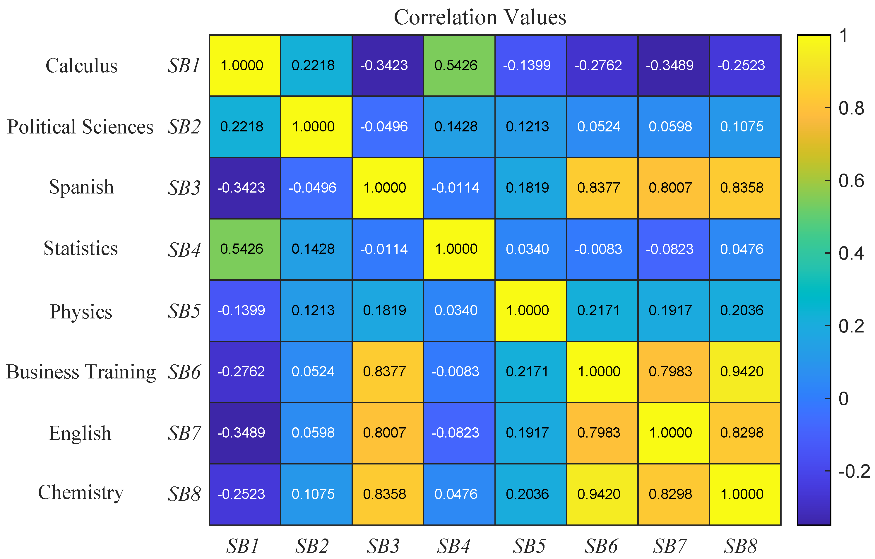
Figure 1 shows the correlation matrix among subjects to identify the relationships of the 11th grade. It should be noted that the calculus subject does not have any type of correlation with other subjects outside of the mathematics area since it is only directly related to statistics; besides, when examining other cells in the calculus row, it is possible to observe that the performance in this area is mostly inversely proportional to the other subjects, which may imply that mathematics requires a high degree of dedication; therefore, when performance increases, other subjects are affected.

On the other hand, the area of languages, which includes English and Spanish, displays a high degree of correlation. In addition, the existing correlation between physics and chemistry is low, which would imply that the only relationship that can exist between these two subjects is the knowledge acquired during the 8th and 9th grades in the sciences subject. One should appreciated that the political science subject does not have any type of relationship with the others.

As a summary of the above, Figure 1 allows knowing the related subjects as observed with $SB3$, $SB6$, $SB7$, and $SB8$; however, when considering the relationship between previous subjects, it should be borne in mind that although there is a high correlation value, there are subjects that do not belong to the same area of knowledge. In this way, subjects that may be affected by common factors such as previously viewed subjects can be established as shown below.

Taking Table 2 and Figure 1 as a reference, it is possible to make the graph of Figure 2, which allows visualizing the learning trajectories for each subject throughout the educational levels proposed, excluding subjects with no high correlation degree or those that, during the teaching process, do not have a relationship between topics. In this way, the relationships among the subjects used to design the prediction system are established.

The information obtained permits the definition of a system where student’s scores can be used by differentiating a unique subject identifier to get a single prediction system instead of multiple systems (one for each subject) working individually.

2.2. Optimization Algorithm Selection

Within the optimization algorithms defined in different documents and investigations, two large groups can be determined. First are algorithms where several N executions provide the same result in the intermediate process and at the end of the execution, which are called deterministic. On the other hand, there are the non-deterministic ones, in which random factors are introduced during the solution search process, for which the same result is not always achieved [21].

Within these groups of non-deterministic algorithms, there are those based on behaviors found in nature, known as metaheuristic algorithms [22], within which it is possible to identify the following:

• Evolutionary algorithms.
• Swarm algorithms.
• Simulated annealing.
• Scattered search.
• Neighborhood search.
• Iterative local search.
• Multi-agent systems.

From the above, different types of optimization algorithms that allow modifying the rules, sets, or parameters of the membership functions of a fuzzy logic system were defined, achieving the prediction of academic performance. For this, the MATLAB Global Optimization Toolbox as used [23]. For the prediction system, the Fuzzy Logic Toolbox was used [24]. Referring to the review of [23], five compatible optimization algorithms were identified, including Genetic Algorithms (GAs), Particle Swarm Optimization (PSO), Simulated Annealing (SA), and Pattern Search (PS).

The toolboxes correspond to Version 2019a, implementing new features within the Fuzzy Logic Toolbox, including the utilization of fuzzy trees as a collection of different fuzzy logic systems or the possibility of carrying out the learning and training process of fuzzy logic systems through some of the algorithms of the Global Optimization Toolbox, such as genetic algorithms, particle swarm optimization, simulated annealing, pattern search, and ANFIS [25].

Genetic algorithms emulate nature’s process of improving a species over time [26,27]. The collective behaviors inspired the algorithms based on swarms of particles that living beings create when searching for food [28,29]. Simulated annealing is a method that aims to emulate the crystalline form of a material by heating and cooling it, thereby seeking to go from a higher to a lower energy state [30]. Pattern search is based on direct search algorithms such as Generalized Pattern Search (GPS), Generating Set Search (GSS), and Mesh Adaptive Search (MADS), where in each step, a mesh pattern of points is generated and evaluated [23].

In this order, the optimization algorithms are used to achieve the objective of modifying the parameters of the proposed fuzzy systems used for the prediction of academic performance.

It is important to note that this work does not seek to make a comparison between algorithms; the object of study is to establish which configuration of the fuzzy system is the most suitable for the prediction system. Under this approach, the most appropriate configuration must present the best performance on the different algorithms used.

2.3. Fuzzy Logic System Design

Fuzzy logic was first proposed in the mid-1960s by Lotfy A. Zadeh, who at that time defined the “principle of incompatibility”. A fuzzy set is a class of objects with different degrees of membership; each set is characterized using different membership functions, which assign to each object a degree of membership in the range between 0 and 1. Using fuzzy logic is beneficial since it represents human reasoning, where the truth or falsity of a proposition, or the degree of belonging of an object to some kind of class, is measured in proportions, such as “little”, “greatly”, “more” and “less” [31].

After carefully analyzing the relevant data and choosing the optimization algorithms, the logic-based system is implemented. The first system designed consisted of multiple inputs and four outputs: each academic period taken by a student during 8th, 9th, and 10th grades corresponded to the system inputs with the number of failures during each elective year and an identifier for the subject. The four outputs corresponded to the prediction of the student’s marks during 11th grade.

For the implementation of the prediction system, a Takagi–Sugeno-type fuzzy inference system was employed, which uses fuzzy sets in the antecedent and, in the output, functions that depend on the input variables [32].

2.4. Takagi–Sugeno Fuzzy Systems

The Takagi–Sugeno fuzzy model was proposed to develop a systematic approach to generating fuzzy rules from a given input-output data set [33]. A typical fuzzy rule in a TS fuzzy model has the form:

If x is A and y is B, then $z=f(x,y)$, where A and B are fuzzy sets in the antecedent and $z=f(x,y)$ is a function in the consequent. In many applications, $f(x,y)$ is a polynomial of inputs x and y. Some TS systems are:

• Zero-order TS fuzzy model: function f is a constant value $f=c$.
• First-order TS fuzzy model: function f is a first-order polynomial $f=ax+by+c$.

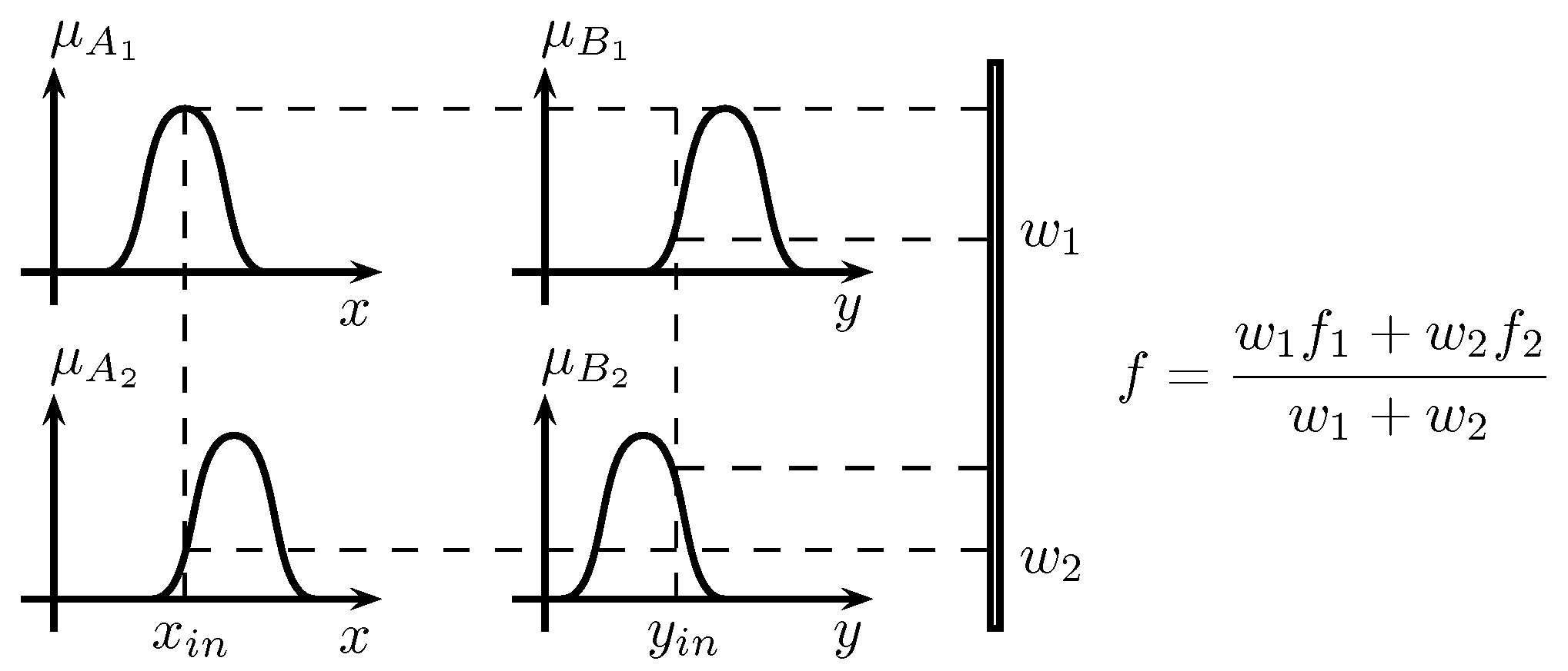
Considering the case when a fuzzy inference system has two inputs x and y and one output z, a first-order TS fuzzy model has rules as follows:

• Rule Number 1: If x is ${\mu }_{A_1}$ and y is ${\mu }_{B_1}$, then $f_1=p_{1}x+q_{1}y+r_1$.
• Rule Number 2: If x is ${\mu }_{A_2}$ and y is ${\mu }_{B_2}$, then $f_2=p_{2}x+q_{2}y+r_2$.

Figure 3 displays an example of a TS fuzzy system for two inputs and two memberships in each input.

2.5. Prediction Models

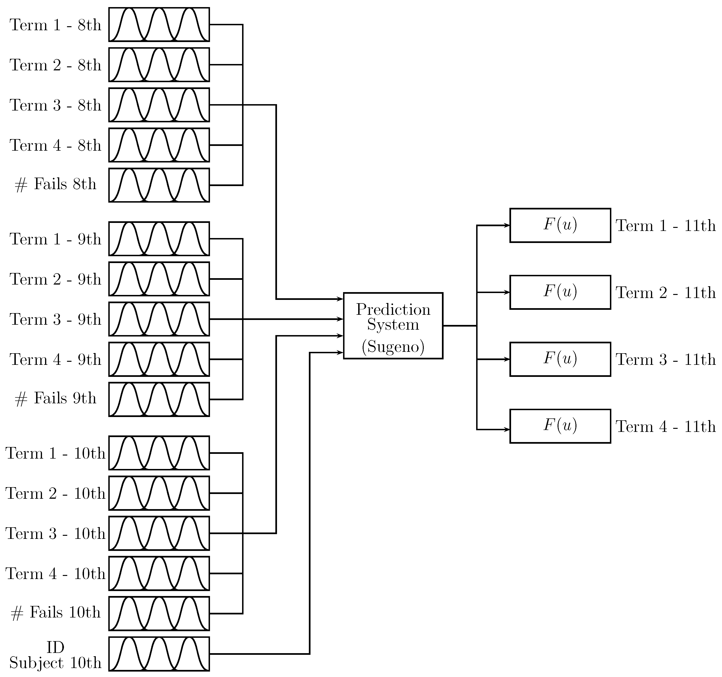
Figure 4 shows the proposed Prediction Model 1 (PM1), which incorporates the inference process into a single zero-order Takagi–Sugeno fuzzy inference system. The system inputs of Figure 4 are the “term” values (student scores) for Periods 1 to 4 of 8th, 9th, and 10th grades. The number of absences “# fails” of the student at the 8th, 9th, and 10th levels is also taken as input; besides, the identifier “ID Subject 10th” is employed (according to Figure 2 and Table 2). The outputs are the predicted term values for Periods 1 to 4 of 11th grade. The “term” scores of the inputs and outputs are values between 0 and 100, the number of absences depending on the number of lectures of the academic period and the subject identifier according to Table 2. In order to reduce the number of inputs, the value of the “final exam” for each level is not included in the prediction system; this can be considered as a system complexity limitation.

By inspecting the proposed system of Figure 4, an overload in the inference process (associated with the number of rules) is established, making it difficult to carry out any modification process and increase the system’s training costs.

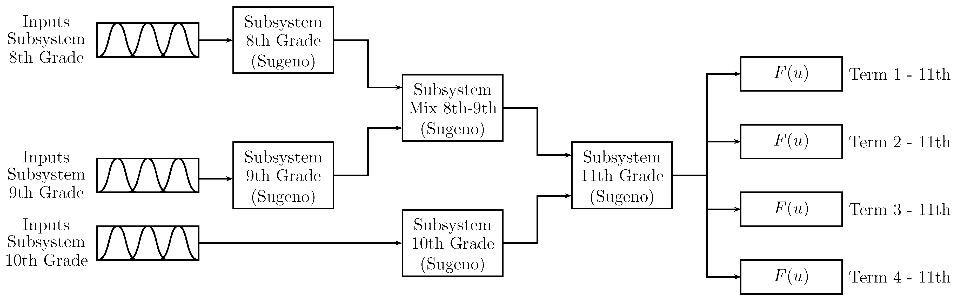
Considering the above, a modular system called Prediction Model 2 (PM2) was developed using zero-order Takagi–Sugeno systems. Each elective grade (level) uses a fuzzy inference system to ease modifications such as when it was necessary to add the qualifications of previous grades to the prediction system. This configuration corresponds to Predictive Model 2 (PM2), shown in Figure 5. Using the systems for each elective grade, the configuration where the subsystems should be placed is shown according to the relationships among them (from Section 2.1).

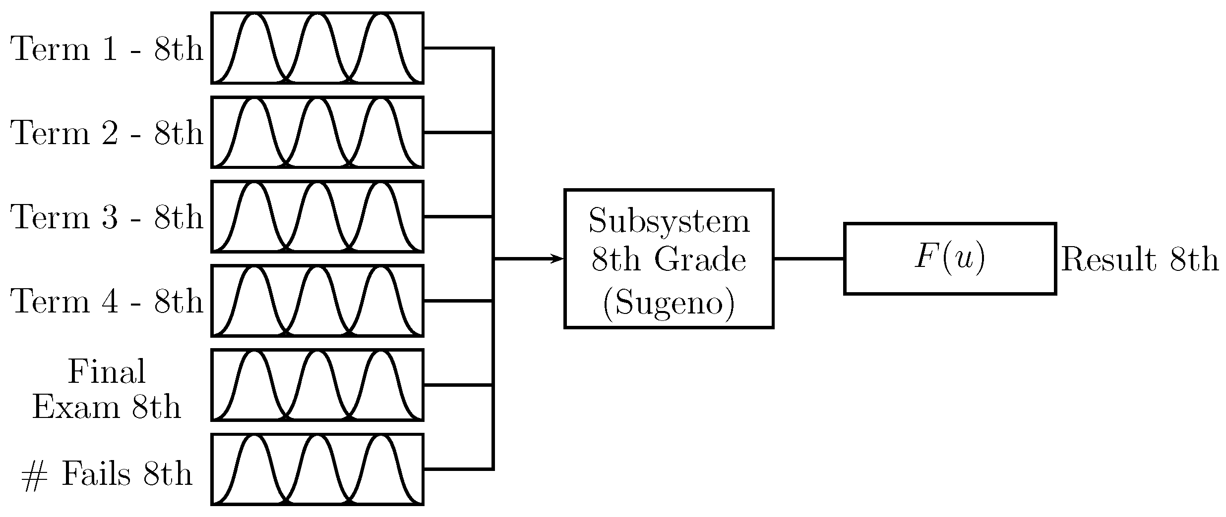
Figure 6 shows the “8th grade” subsystem; the inputs are the “term” values of students’ grades for Periods 1 to 4, including the mark for the “final exam” and the student’s number of absences “# fails”. The output corresponds to the influence of this subsystem on the prediction. The “term” inputs, the “final exam”, and the output have values between $[0,100]$.

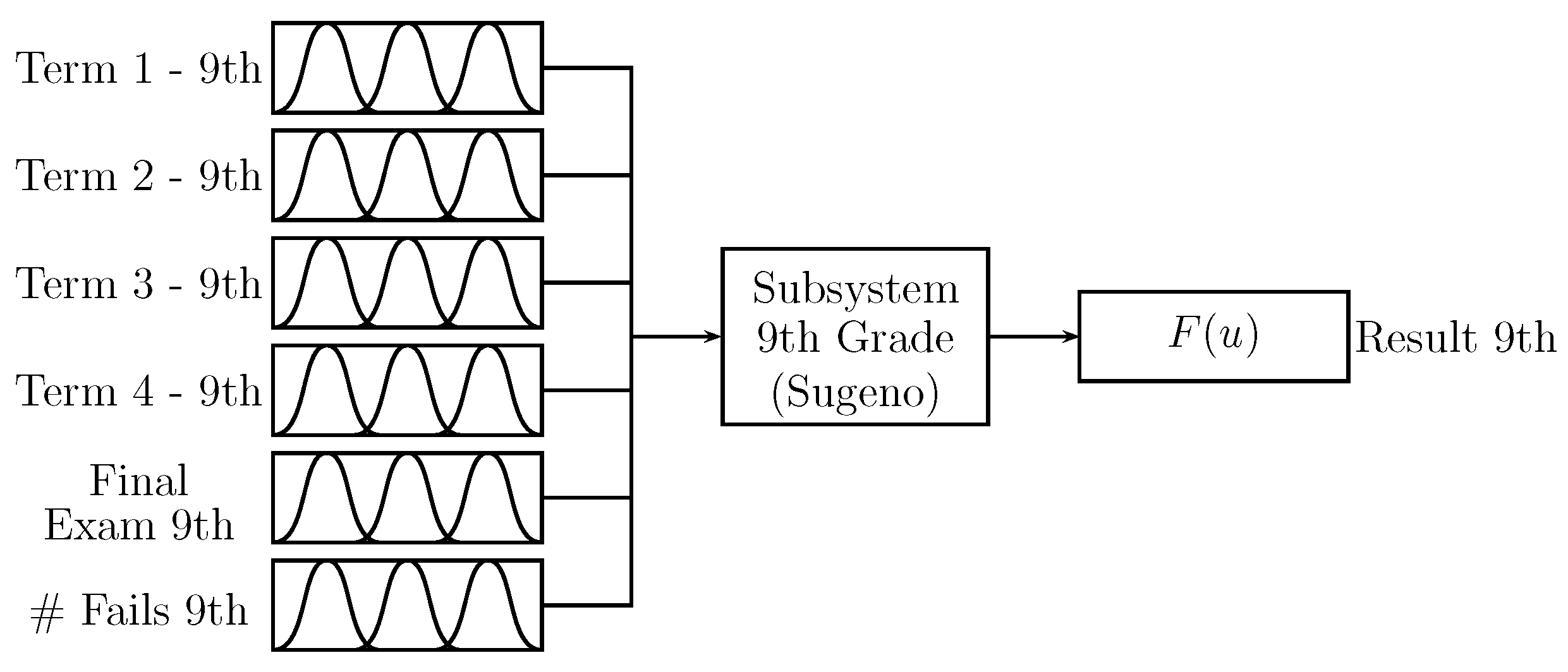
Figure 7 shows the “9th grade” subsystem with the same structure of the “8th grade” subsystem; however, for this, the data of 9th grade is used. The output “Result 9th” is a value in the range $[0,100]$.

Figure 8 shows the configuration for the subsystem associated with 10th grade. The system inputs are the “term” values obtained by the students in Periods 1 to 4, the “final exam” also being used as input with vales between 0 and 100. The number of students’ absences for each grade “# fails” and, as additional input, the identification of the subject type “ID subject” are shown according to Table 2. The subject identifier is included in this system since the trigonometry and statistics subjects of 10th grade have an influence on 11th grade statistics, as presented in Figure 2.

As observed in Figure 5, the creation of a combination subsystem was proposed where the outputs of the subsystems “8th grade”, and “9th grade” are used to obtain a single output. The range of values for the inputs and output of the subsystem “mixed 8th–9th” is $[0,100]$. In the same way, the subsystem “11th grade” uses the outputs of subsystems “mixed 8th–9th” and “10th grade” to attain the “term” prediction values of “11th Grade” for each of Period 1 to 4. The range of values for the inputs and output of this subsystem is $[0,100]$.

As functioning example is considered as the case of one student that has the scores presented in

Table 3. Data input and output example for 11th grade chemistry.

Features	Grade (Input)			Result (Output)
(Inputs)	8th	9th	10th	11th
Term 1	83.50	87.00	92.33	81.00
Term 2	82.00	76.75	89.00	80.00
Term 3	70.50	70.00	84.00	76.67
Term 4	86.25	79.50	89.00	94.00
Final Exam	85.00	86.00	72.00	-
# Fails	6	1	1	-
ID Subject	-	-	1	-

, where the columns of 8th, 9th, and 10th grade contain the data input and the column for 11th grade the resulting output.

2.6. System Optimization

The implementation seeks to establish which configuration of the fuzzy system presents the best result for the different algorithms considered. Thus, according to the number of rules used in the fuzzy systems, the same trend must be presented in the algorithms used.

For the optimization process, the four selected algorithms were implemented in the fuzzy logic tree proposed in Figure 5. For PM2, two-hundred iterations were carried out for each algorithm, and five different scenarios were proposed, each one with a maximum number of rules (5, 10, 20, 50, and 70). This represents the maximum number of rules assigned within each of the subsystems (8th, 9th, 8th–9th, 10th, 11th); this is in order to find the point at which the number of rules ceases to strongly influence the error of the predictions.

For the optimization algorithms, some important factors can affect their efficiency. In this regard, different approaches for parameter selection can be considered as presented in [34,35,36], where the common approach was via meta-optimization. In particular, suggestions for GA parameter selection can be found in [37], as well as in [38] for PSO and in [39] for SA. However, as the objective of this work is not to carry out a study of the parameter variation of the optimization algorithms, for the configuration of these algorithms, the suggestions (default parameters) of [40] for the GA and those in [41] for PSO, SA, and PS were followed, which are presented below.

For the GA, the size of the population is 200; the crossover fraction was set to $0.8$; and the mutation rate was equal to $0.01$; for coding solutions (chromosome), the type “double” data in MATLAB was used, which is a 64 bit word with 1 sign bit, 11 bits for floating point exponent, and 52 bits for the mantissa; in addition, for the rule list, a “bit string” was used. The scattered crossover function was used, which creates a random binary vector and selects the genes where the vector is 1 from the first parent and the genes where the vector is 0 from the second parent, combining the genes to create the offspring. In addition, the Gaussian mutation function was used, for which a random number taken from a Gaussian distribution was used for the mutation process, and the Gaussian distribution depended on the parameters’ scale and the population range. The algorithm stops if the average relative change in the best fitness function is less than $1\times {10}^{-6}$. For PSO, the swarm size was $10n_{var}$, where $n_{var}$ is the number of variables of the fuzzy model, and the cognitive (self-adjustment) weight associated with each particle’s best position was set to $1.49$, while the social adjustment weight associated with best position of the swarm was equal to $1.49$. Using SA, the initial $T_0$ temperature was set to 100 for each dimension, while the reannealing interval corresponded to 50. The function used to update the temperature schedule was $T\left(k\right)=0.{95}^k$, where k is the annealing parameter. Finally, for PS, the initial mesh size was set to 10, and the mesh tolerance value used to stop the sear process was $1\times {10}^{-7}$.

Table 4. Optimization results using genetic algorithms.

-	5		10		20		50		70
-	Rules		Rules		Rules		Rules		Rules
Number of	Best	Mean	Best	Mean	Best	Mean	Best	Mean	Best	Mean
Generations	$\mathit{f}\left(\mathit{X}\right)$	$\mathit{f}\left(\mathit{X}\right)$	$\mathit{f}\left(\mathit{X}\right)$	$\mathit{f}\left(\mathit{X}\right)$	$\mathit{f}\left(\mathit{X}\right)$	$\mathit{f}\left(\mathit{X}\right)$	$\mathit{f}\left(\mathit{X}\right)$	$\mathit{f}\left(\mathit{X}\right)$	$\mathit{f}\left(\mathit{X}\right)$	$\mathit{f}\left(\mathit{X}\right)$
1	18.5	36.75	22.08	36.92	19.03	35.08	19.58	34.9	18.93	34.82
5	17.34	27.54	17.24	29.78	16.96	28.03	15.8	29.2	17.16	27.75
10	15.63	21.95	14.23	20.17	13.37	24.76	14.06	21.62	13.37	22.72
50	11.4	11.85	9.405	9.841	8.379	8.737	9.648	9.956	8.204	8.337
80	11.4	11.4	9.333	9.558	7.712	8.066	8.288	8.583	7.786	7.988
90	11.4	11.4	9.322	9.641	7.51	7.793	7.93	8.26	7.732	7.824
100	11.4	11.4	9.314	9.569	7.487	7.725	7.772	7.955	7.526	7.677
150	-	-	9.3	9.74	7.375	8.27	7.339	7.48	7.065	7.224
200	-	-	9.296	9.561	7.339	7.698	7.225	7.278	7	7.054

,

Table 5. Optimization results using particle swarm optimization.

-	5		10		20		50		70
-	Rules		Rules		Rules		Rules		Rules
Number of	Best	Mean	Best	Mean	Best	Mean	Best	Mean	Best	Mean
Iterations	$\mathit{f}\left(\mathit{X}\right)$	$\mathit{f}\left(\mathit{X}\right)$	$\mathit{f}\left(\mathit{X}\right)$	$\mathit{f}\left(\mathit{X}\right)$	$\mathit{f}\left(\mathit{X}\right)$	$\mathit{f}\left(\mathit{X}\right)$	$\mathit{f}\left(\mathit{X}\right)$	$\mathit{f}\left(\mathit{X}\right)$	$\mathit{f}\left(\mathit{X}\right)$	$\mathit{f}\left(\mathit{X}\right)$
1	21.53	40.44	19.29	37.04	17.49	35.37	17.1	33.68	17.96	33.44
5	17.28	35.27	17.53	33.97	16.74	30.75	17.1	32.26	16.04	29.42
10	17.28	35.95	16.25	32.34	16.38	30.05	16.19	30.6	16.04	27.09
50	13.05	20.38	11.74	18.6	10.48	19.18	11.63	24.65	8.565	16.24
80	13.03	14.84	11.67	17.38	8.467	13.49	10.59	16.82	7.688	12.24
90	13.03	15.14	10.92	15.26	8.43	14.68	10.7	16.82	7.492	11.2
100	13.03	15.04	9.707	19.84	8.215	12.09	10.33	16.24	7.373	9.977
150	13	14	9.348	11.74	7.893	9.314	9.906	18.63	7.25	10.83
160	13	13.85	9.337	10.79	7.813	12.55	9.827	13.79	7.237	8.013
190	-	-	9.175	9.936	7.724	9.467	9.634	13.98	7.198	7.802
200	-	-	9.174	10.14	7.72	12.97	9.599	13.39	7.196	8.773

,

Table 6. Optimization results using simulated annealing.

-	5		10		20		50		70
-	Rules		Rules		Rules		Rules		Rules
Number of	Best	Mean	Best	Mean	Best	Mean	Best	Mean	Best	Mean
Iterations	$\mathit{f}\left(\mathit{X}\right)$	$\mathit{f}\left(\mathit{X}\right)$	$\mathit{f}\left(\mathit{X}\right)$	$\mathit{f}\left(\mathit{X}\right)$	$\mathit{f}\left(\mathit{X}\right)$	$\mathit{f}\left(\mathit{X}\right)$	$\mathit{f}\left(\mathit{X}\right)$	$\mathit{f}\left(\mathit{X}\right)$	$\mathit{f}\left(\mathit{X}\right)$	$\mathit{f}\left(\mathit{X}\right)$
1	24.38	29.37	33.29	33.29	27.82	29.22	26.5	26.5	41.45	41.44
5	24.38	46.64	21.69	26.53	21.64	35.06	26.5	42.88	19.99	22.56
10	24.38	36.78	21.69	22.68	21.64	30.23	26.5	36.12	19.99	24.06
50	19.38	25.2867	16.07	18.82	17.94	29.59	22.66	24.96	19.44	19.44
100	19.38	35.73	16.07	20.76	16.03	33.02	20.39	30.93	18.95	20.6
150	17.75	36.28	16.07	32.04	16.03	29.66	20.39	41.83	18.95	34.86
200	17.75	33.26	16.07	25.61	16.03	33.25	20.39	33.68	18.04	18.09

and

Table 7. Optimization results using pattern search.

-	5		10		20		50		70
Number of	Rules		Rules		Rules		Rules		Rules
Iterations	$\mathit{f}\left(\mathit{X}\right)$	Size Grid	$\mathit{f}\left(\mathit{X}\right)$	Size Grid	$\mathit{f}\left(\mathit{X}\right)$	Size Grid	$\mathit{f}\left(\mathit{X}\right)$	Size Grid	$\mathit{f}\left(\mathit{X}\right)$	Size Grid
1	59.45	2	59.45	2	59.45	2	59.45	2	59.45	2
5	35.21	2	35.21	2	35.21	2	35.21	2	35.21	2
10	16.77	1	16.77	1	16.77	1	16.77	1	16.77	1
15	16.77	0.125	16.77	0.125	16.77	0.125	16.77	0.125	16.77	0.125
20	16.77	0.004	16.77	0.004	16.77	0.004	16.77	0.004	16.77	0.004
25	16.77	0.0001	16.77	0.0001	16.77	0.0001	16.77	0.0001	16.77	0.0001
30	16.77	$3.80\times {10}^{-6}$	16.77	$3.80\times {10}^{-6}$	16.77	$3.80\times {10}^{-6}$	16.77	$3.80\times {10}^{-6}$	16.77	$3.80\times {10}^{-6}$
32	16.77	$9.50\times {10}^{-7}$	16.77	$9.50\times {10}^{-7}$	16.77	$9.50\times {10}^{-7}$	16.77	$9.50\times {10}^{-7}$	16.77	$9.50\times {10}^{-7}$

show a summary of the results obtained during the optimization process. On the other hand, setting 200 iterations allows finding the one where the variation of the error between the iterations is no longer significant with respect to the time it takes to execute each iteration.

The objective function is presented in Equation (2), where i is the variable associated with each input-output data, N the total number of data used, $Rea{l}_i$ the value of the real data, $Calculate{d}_i\left(X\right)$ the data obtained using the prediction fuzzy system, and X the parameters of the fuzzy system that include the parameters of the membership functions, the rules of the fuzzy system, and the parameters of the output functions of each Sugeno-type fuzzy subsystem.

$$f\left(X\right)=\sqrt{\frac{1}{N}\sum _{i=1}^N{(Rea{l}_i-Calculate{d}_i\left(X\right))}^2}$$

(2)

As seen in Table 4, during the optimization process of the system with 5 rules, a minimum error of $11.4$ points was reached. On the other hand, the system with 70 rules managed to obtain the lowest error during 200 generations, although it was not possible to capture a significant variation of this after the 150th generation. Finally, the systems with 5 and 10 rules, during optimization, presented alerts due to the lack of rules associated with system outputs.

By analyzing the results obtained during the optimization process with the particle swarm optimization shown in Table 5, it can be seen that the system with 5 rules ended prematurely in Iteration 160, in turn obtaining the worst error of the algorithm, while the system with 70 rules achieved the best result in Generation 190, with a mean error of 7.8.

When analyzing the results obtained by the optimization process using the simulated annealing algorithm (Table 6), it is seen that during several iterations, there was no reduction in error, and in turn, the algorithm attained the worst optimization result.

According to Table 7, the pattern search optimization algorithm produces the same error of 16.77 in all systems. For the adaptive mesh pattern search algorithm, regardless of the maximum number of rules, the system always ended when reaching 32 iterations because the minimum size for the mesh was reached, which is located below $1.0\times {10}^{-8}$.

3. Result Analysis

For the result analysis, the measures of the Mean Absolute Deviation (MAD), the Root Mean Squared Error (RMSE), and the Symmetric Mean Absolute Percentage Error (SMAPE) were used [42]. The MAD measure is the mean of the absolute deviations of a dataset about the data’s mean, and this corresponds to the average distance of the data set from its mean and is defined as:

$$MAD=\frac{{\displaystyle \sum _{i=1}^N}|Rea{l}_i-Calculate{d}_i|}{N}$$

(3)

The mean squared error is commonly used for assessing numeric prediction. This value is computed by taking the squared differences between each predicted value and the actual value. Thus, the root mean squared error corresponds to the square root of the mean squared error, given by the formula:

$$RMSE=\sqrt{\frac{{\displaystyle \sum _{i=1}^N}{(Rea{l}_i-Calculate{d}_i)}^2}{N}}$$

(4)

The mean absolute percentage error is a measure of accuracy in fitted dataset values, and this performance measure usually expresses accuracy as a percentage, calculated by the following expression:

$$SMAPE=\frac{100\%}{N}{\displaystyle \sum _{i=1}^N}\frac{|Rea{l}_i-Calculate{d}_i|}{|Rea{l}_i|+|Calculate{d}_i|}$$

(5)

In the above equations, i is the index of the data value, $Rea{l}_i$ corresponds to the real data, $Calculate{d}_i$ is the value calculated with the fuzzy inference system, and N is the total number of data.

The MAD and RMSE are used to make precision comparisons between different algorithms, while the SMAPE allows evaluating the error percentage in the predictions considering only its magnitude.

Furthermore, a comparison was made between the predictions by each of the algorithms implemented, in such a way that the best algorithm could be selected, as well as the best number of rules for the system. The following tables present the results obtained by the MAD, RMSE, and SMAPE measurements; on the other hand, each table indicates the maximum number of rules associated with the learning and optimization process. As a note, the SMAPE is given in terms of the percentage of error.

Table 8. Error measurement considering different numbers of rules. PS, Pattern Search; SMAPE, Symmetric Mean Absolute Percentage Error.

5 Rules
Measure	GA	PSO	SA	PS
MAD	10.415	10.5289	14.1012	13.7737
RMSE	13.1114	12.7891	16.8512	15.9708
SMAPE	16.04%	15.49%	21.58%	20.99%
10 Rules
Measure	GA	PSO	SA	PS
MAD	6.8494	8.0779	13.2082	13.7737
RMSE	9.0726	9.976	15.3469	15.9708
SMAPE	10.16%	12.40%	20.19%	20.99%
20 Rules
Measure	GA	PSO	SA	PS
MAD	5.4282	5.9044	13.6077	13.7737
RMSE	7.4833	8.1553	15.8417	15.9708
SMAPE	8.32%	9.13%	21.30%	20.99%
50 Rules
Measure	GA	PSO	SA	PS
MAD	5.5452	7.6017	17.5366	13.7737
RMSE	7.7689	9.7637	20.1783	15.9708
SMAPE	8.69%	11.81%	28.31%	20.99%
70 Rules
Measure	GA	PSO	SA	PS
MAD	5.3774	5.4175	15.0029	13.7737
RMSE	7.6123	7.6526	17.3534	15.9708
SMAPE	8.38%	8.38%	22.70%	20.99%

presents the summary of the results obtained by the system during the optimization process. From all data, seventy-two percent (121 input-output data) of the total data was used to perform the system training, while the remaining $28\%$ (47 input-output data) was used to perform the system evaluation process.

When analyzing the results, it is possible to see the lowest error percentage achieved where the genetic algorithms were implemented during the optimization process; meanwhile, the worst results are attributed to the simulated annealing algorithm and pattern search.

Subsequently,

Table 9. Comparison of the errors for 20 and 70 rules.

-	Output
Measure	Mark 1	Mark 2	Mark 3	Mark 4
MAD for 20 R	4.8728	5.0576	7.6355	4.1469
MAD for 70 R	5.2924	5.4486	7.1452	3.6234
RMSE for 20 R	6.3535	6.673	10.7386	4.877
RMSE for 70 R	6.6572	7.5007	10.44	4.7133
SMAPE for 20 R	7.64%	8.62%	11.25%	5.78%
SMAPE for 70 R	8.28%	9.35%	10.76%	5.15%

describes the analysis of the results considering the maximum number of rules for the system, and from there, the system is visualized, in which a maximum of 70 rules were used presenting the lowest MAD, followed by the set of 20 rules. Then, the evaluation process of both systems took place using the remaining $28\%$ of the data, in turn analyzing the error for each of the outputs individually.

When checking the results obtained during the system evaluation process, it is seen that the system in which a maximum number of 20 rules obtained the lowest error for the first two outputs, this corresponds to the first and second academic periods of 11th grade, with an error around $4.87$ and $5.1$ points. Analyzing the SMAPE, it would correspond to an error of $7.6\%$ and $8.6\%$, respectively.

On the other hand, the system with 70 rules managed to obtain the best result for the third and fourth academic periods with an approximate error percentage of $10.8\%$ and $5.15\%$; therefore, when compared to the results obtained by the system with 20 rules, it is not possible to really appreciate a difference high enough to define without further analysis any of these two systems.

Besides, to determine a suitable prediction system, it is necessary to consider the time required for the system optimization process. For this,

Table 10. Execution time for the optimization process in minutes.

Rules	GA	PSO	SA	PS
5	30.08	23.89	4.21	6.48
10	81.40	43.46	10.98	23.47
20	190.78	89.34	38.93	98.86
50	610.77	273.19	288.67	828.35
70	1007.98	447.24	636.74	1945.20

was calculated, presenting the respective time for each algorithm and different numbers of rules. In order to unify the execution of GA, PSO, and SA algorithms, two-thousand iterations were used in each case. For PS, it stopped at Iteration 34, inasmuch as the smallest mesh of $9.537\times {10}^{-7}$ was reached. Since the best results of MAD, RMSE, and SMAPE were obtained for 20 and 70 rules using GA, then during the system’s optimization process using GA with 20 rules, it spent 190.78 minutes. Meanwhile, the system of 70 rules took 1007.98 minutes. Then, considering this aspect, the system based on 20 rules is the suitable option, since it uses low optimization time.

4. Discussion

Despite the different system implementations made, the genetic algorithms managed to reach the best result. Contrary to the expectations, the implementation with a maximum of 20 rules per subsystem managed to obtain a better result than the one with 70 rules, and this is because the latter required a greater number of generations for a better product, although this requires a high computational and temporal cost.

On the other hand, when analyzing the amount of rules generated in each subsystem, it was seen that the greatest computational load in terms of the optimization process occurred in the first three subsystems since they were the ones using the maximum limit of rules, while the last two reached less than $50\%$ of the maximum amount.

Regarding the error measurement, a suitable performance was obtained since the MAD was located at 5.4282 and the RMSE at 7.4833. Using an evaluation scale that goes from zero to 100, the error was less than $10\%$, which is a positive aspect given the difficulty of predicting data such as academic performance.

The error obtained was acceptable since it was expected to execute a academic control on those students displaying low performance during the last academic period. The proposed system provided a preview of students’ performance; when implementing this system with one of the alerts, it notifies about the student’s low performance or possible academic problems from the beginning.

The proposed model is applicable to all educational levels, which implies a fine-tuned monitoring and academic control provided that the intervention is suitable and adequate. Implementing this intervention must be based on the expected profiles of a person at each educational stage; mainly, it is necessary to define the advancements of the student’s when finishing each level. From this viewpoint, the educational strategies constitute the best answer to meet the educational needs. These may be easier if the profiles are synchronously obtained with the learning and development of skills and competencies in building a disciplinary lifestyle.

Finally, it should be considered that a direct comparison between the algorithms was not carried out since the object of study was to establish the most appropriate configuration of the fuzzy prediction system. The optimization algorithms allow observing the existence of a configuration that presents the best result for the different algorithms considered.

5. Conclusions

The study would allow academic control either by carrying out reinforcements at the beginning of the year or by notifying the parents about the shortcomings that the student may have throughout the year, in such a way that some difficulties are mitigated, allowing the institution to achieve better outcomes from the state tests, granting a better reputation to the institution due to its educational quality and the high effectiveness of the communication process between the institution and parents regardless of the shortcomings of the learners.

It is also observed that students’ academic performance depends on a large number of external factors that affect students in positive and negative ways, like health status or even mood. Therefore, taking into account that these factors were not considered, it is concluded that a suitable error result was achieved, which can be improved if more variables are added to the system, although these would lead to a higher computational cost.

Finally, the implementation costs were not high since they only require the energy expenditure of the remote server that performs the optimization process, and the time cost depends directly on the machine where the process is executed; thus, based on the fact that a 2.0GHz quad-core computer spends approximately four hours on optimization using genetic algorithms with 20 rules for each subsystem with 200 records divided between training and evaluation data.

References

- Umbleja, K. Students grading control and visualization in competence- based learning approach. In Proceedings of the 2015 IEEE Global Engineering Education Conference (EDUCON), Tallinn, Estonia, 18–20 March 2015; pp. 287–296. [Google Scholar]
- Hameed, A. Enhanced fuzzy system for students’ academic evaluation using linguistic hedges. In Proceedings of the 2017 IEEE International Conference on Fuzzy Systems (FUZZ-IEEE), Naples, Italy, 9–12 July 2017; pp. 1–6. [Google Scholar]
- Arsad, P.M.; Buniyamin, N.; Manan, J.A. Prediction of engineering students’ academic performance using Artificial Neural Network and Linear Regression: A comparison. In Proceedings of the 2013 IEEE 5th Conference on Engineering Education (ICEED), Kuala Lumpur, Malaysia, 4–5 December 2018; pp. 43–48. [Google Scholar]
- Li, Z.; Shang, C.; Shen, Q. Fuzzy-clustering embedded regression for predicting student academic performance. In Proceedings of the 2016 IEEE International Conference on Fuzzy Systems (FUZZ-IEEE), Vancouver, BC, Canada, 24–29 July 2016; pp. 344–351. [Google Scholar]
- Merchan-Rubiano, S.M.; Duarte-Garcia, J.A. Formulation of a predictive model for academic performance based on students’ academic and demographic data. In Proceedings of the 2015 IEEE Frontiers in Education Conference (FIE), El Paso, TX, USA, 21–24 October 2015; pp. 1–7. [Google Scholar]
- Merchan-Rubiano, S.M.; Duarte-Garcia, J.A. Analysis of Data Mining Techniques for constructing a Predictive Model for Academic Performance. IEEE Lat. Am. Trans. 2016, 14, 2783–2788. [Google Scholar] [CrossRef]
- Kaunang, F.M.; Rotikan, R. Students’ Academic Performance Prediction using Data Mining. In Proceedings of the Third International Conference on Informatics and Computing (ICIC), Palembang, Indonesia, 17–18 October 2018; pp. 1–5. [Google Scholar]
- Tikhomirova, T.; Malykh, A.; Malykh, S. Predicting Academic Achievement with Cognitive Abilities: Cross-Sectional Study across School Education. Behav. Sci. 2020, 10, 158. [Google Scholar] [CrossRef] [PubMed]
- Sánchez-Serrano, J.; Jaén-Martínez, A.; Montenegro-Rueda, M.; Fernández-Cerero, J. Impact of the Information and Communication Technologies on Students with Disabilities. A Systematic Review 2009–2019. Sustainability 2020, 12, 8603. [Google Scholar] [CrossRef]
- Retuerto, D.M.; Martínez de Lahidalga, I.R.; Ibañez-Lasurtegui, I. Disruptive Behavior Programs on Primary School Students: A Systematic Review. Eur. J. Investig. Health Psychol. Educ. 2020, 10, 995–1009. [Google Scholar] [CrossRef]
- Lee, T.S.; Wang, C.H.; Yu, C.M. Fuzzy Evaluation Model for Enhancing E-Learning Systems. Mathematics 2019, 7, 918. [Google Scholar] [CrossRef]
- Takagi, T.; Sugeno, M. Fuzzy identification of systems and its applications to modelling and control. IEEE Trans. Syst. Man Cybern. 1985, 15, 116–132. [Google Scholar] [CrossRef]
- Castillo, O.; Valdez, F.; Soria, J.; Yoon, J.H.; Geem, Z.W.; Peraza, C.; Ochoa, P.; Amador-Angulo, L. Optimal Design of Fuzzy Systems Using Differential Evolution and Harmony Search Algorithms with Dynamic Parameter Adaptation. Appl. Sci. 2020, 10, 6146. [Google Scholar] [CrossRef]
- Aguilar-Salinas, W.; Ojeda-Benitez, S.; Cruz-Sotelo, S.E.; Castro-Rodríguez, J.R. Model to Evaluate Pro-Environmental Consumer Practices. Environments 2017, 4, 11. [Google Scholar] [CrossRef]
- Ain, Q.-U.; Iqbal, S.; Khan, S.A.; Malik, A.W.; Ahmad, I.; Javaid, N. IoT Operating System Based Fuzzy Inference System for Home Energy Management System in Smart Buildings. Sensors 2018, 18, 2802. [Google Scholar] [CrossRef] [PubMed]
- Alawad, H.; An, M.; Kaewunruen, S. Utilizing an Adaptive Neuro-Fuzzy Inference System (ANFIS) for Overcrowding Level Risk Assessment in Railway Stations. Appl. Sci. 2020, 10, 5156. [Google Scholar] [CrossRef]
- Fale, M.I.; Abdulsalam, Y.G. Dr. Flynxz-A First Aid Mamdani-Sugeno-type fuzzy expert system for differential symptoms-based diagnosis. J. King Saud Univ. Comput. Inf. Sci. 2020. [Google Scholar] [CrossRef]
- MINEDUCACIÓN. Colombian Education System. 2019. Available online: https://www.mineducacion.gov.co/1759/w3-article-355502.html?_noredirect=1 (accessed on 17 March 2020).
- ICFES, MINEDUCACIÓN. Guía de Orientación-Saber 9. 2017. Available online: https://www.icfes.gov.co/documents/20143/1353827/Guia+de+orientacion+saber+9+2017.pdf/fdf46960-c1d4-96b2-ef0d-78b4c885bfcc (accessed on 17 March 2020).
- ICFES MINEDUCACIÓN. Guía de Orientación-Saber 11. 2020. Available online: https://www.icfes.gov.co/documents/20143/1628228/Guia+de+orientacion+saber+11+2020-1.pdf/ec534dff-b171-d51b-5ee8-c05139100635 (accessed on 17 March 2020).
- Esmorís, A.V. Algoritmos Heurísticos en Optimización. Master’s Thesis, Universidad de Santiago de Compostela, Santiago de Compostela, Spain, 2013. [Google Scholar]
- Duarte, A.; Gallego, M.; Pantrigo, J. Metaheurísticas; Dykinson: Madrid, Spain, 2007. [Google Scholar]
- MathWorks, Global Optimization Toolbox. Available online: https://www.mathworks.com/products/global-optimization.html (accessed on 20 March 2020).
- MathWorks, Fuzzy Logic Toolbox. Available online: https://www.mathworks.com/products/fuzzy-logic.html (accessed on 20 March 2020).
- MathWorks, Fuzzy Logic Toolbox Release Notes. Available online: https://www.mathworks.com/help/fuzzy/release-notes.html (accessed on 20 March 2020).
- Wirsansky, E. Hands-On Genetic Algorithms with Python: Applying Genetic Algorithms to Solve Real-World Deep Learning and Artificial Intelligence Problems; Packt Publishing: Birmingham, UK, 2020. [Google Scholar]
- Dehghani, M.; Montazeri, Z.; Dhiman, G.; Malik, O.P.; Morales, R.; Ramirez, R.A.; Dehghani, A.; Guerrero, J.M.; Parra, L. A Spring Search Algorithm Applied to Engineering Optimization Problems. Appl. Sci. 2020, 10, 6173. [Google Scholar] [CrossRef]
- Clerc, M. Particle Swarm Optimization; John Wiley & Sons: London, UK, 2013. [Google Scholar]
- Llama, M.; Flores, A.; Garcia, R.; Santibañez, V. Heuristic Global Optimization of an Adaptive Fuzzy Controller for the Inverted Pendulum System: Experimental Comparison. Appl. Sci. 2020, 10, 6158. [Google Scholar] [CrossRef]
- Almarashi, M.; Deabes, W.; Amin, H.H.; Hedar, A.R. Simulated Annealing with Exploratory Sensing for Global Optimization. Algorithms 2020, 13, 230. [Google Scholar] [CrossRef]
- Kerre, E.E.; Mordeson, J. Fuzzy Mathematics; MDPI: Basel, Switzerland, 2018. [Google Scholar]
- Espitia, H.; Soriano, J.; Machón, I.; López, H. Design Methodology for the Implementation of Fuzzy Inference Systems Based on Boolean Relations. Electronics 2019, 8, 1243. [Google Scholar] [CrossRef]
- Jang, J.S.R.; Sun, C.T.; Mizutani, E. Neuro-Fuzzy and Soft Computing: A Computational Approach to Learning and Machine Intelligence; Prentice Hall: Upper Saddle River, NJ, USA, 1997. [Google Scholar]
- Neumüller, C.; Wagner, S.; Kronberger, G.; Affenzeller, M. Parameter Meta-optimization of Metaheuristic Optimization Algorithms. Lect. Notes Comput. Sci. 2012, 6927, 367–374. [Google Scholar] [CrossRef]
- López, M.; Dubois, J.; Pérez, L.; Stützle, T.; Birattari, M. The irace package: Iterated Racing for Automatic Algorithm Configuration. Oper. Res. Perspect. 2016, 3, 43–58. [Google Scholar] [CrossRef]
- Bozorg, O.; Solgi, M.; Loáiciga, H. Meta-Heuristic and Evolutionary Algorithms for Engineering Optimization; Wiley: Hoboken, NJ, USA, 2017. [Google Scholar]
- Angelova, M.; Pencheva, T. Tuning Genetic Algorithm Parameters to Improve Convergence Time. Int. J. Chem. Eng. 2011, 646917. [Google Scholar] [CrossRef]
- Zhang, W.; Ma, D.; Wei, J.; Liang, H. A parameter selection strategy for particle swarm optimization based on particle positions. Expert Syst. Appl. 2014, 41, 3576–3584. [Google Scholar] [CrossRef]
- Weyland, D. Simulated annealing, its parameter settings and the longest common subsequence problema. In Proceedings of the GECCO’08, 10th Annual Conference on Genetic and Evolutionary Computation, Atlanta, GA, USA, 12–16 July 2008; pp. 803–810. [Google Scholar]
- MathWorks. Genetic Algorithm and Direct Search Toolbox, For Use with MATLAB®. In MathWorks User’s Guide, Version 1; MathWorks: Natick, MA, USA, 2004. [Google Scholar]
- MathWorks. Global Optimization Toolbox User’s Guide. In MathWorks; MathWorks: Natick, MA, USA, 2015. [Google Scholar]
- Olatunji, S.O.; Al-Ahmadi, M.S.; Elshafei, M.; Fallatah, Y.A. Forecasting the Saudi Arabia stock prices based on artificial neural networks model. Int. J. Intell. Inf. Syst. 2013, 2, 77–86. [Google Scholar] [CrossRef][Green Version]