Simulation Methodology-Based Context-Aware Architecture Design for Behavior Monitoring of Systems

Abstract

Generally, simulation models are constructed to replicate and predict the behavior of real systems that currently exist or are expected to exist in the future. Once a simulation model is implemented, the model can be connected to a real system for which the model has been built through sensors or networks so that important activities in the real system can be monitored indirectly through the model. This article proposes a modeling formalism BM-DEVS (Behavior Monitor-DEVS) that defines simulation models capable of monitoring the desired behavior patterns within the models so that the target system’s behavior can be monitored indirectly. In BM-DEVS, an extension of classic Discrete Event System Specification (DEVS), the behavior to be monitored is expressed as a set of temporal logic (TL) production rules within a multi-component model that consists of multiple component models to be monitored. An inference engine module for reasoning with the TL rules is designed based on the abstract simulator that carries out instructions in the BM-DEVS models to perform the simulation process. The major application of BM-DEVS is in the design and implementation of the context-aware architecture needed for various intelligent systems as a core constituent. Essentially all systems where some form of behavior monitoring is required are candidate applications of BM-DEVS. This research is motivated by the view that there exists symmetry between the real-world and the cyber world, in that the problems in both environments should be expressed with the same basic constituents of time and space; this naturally leads to adopting spatiotemporal variables composed of simulation models and developing a problem solver that exploits these variables.

1. Introduction

Smart systems require the acquisition of various information or data to monitor the behavior of their environment. Such systems include smart buildings, smart agricultural fields, smart homes, and smart vehicles [1,2,3]. Especially, environment behavioral knowledge is an essential part of such smart systems, including context-aware systems for various purposes [3,4,5,6,7,8]. The smartness level can be enhanced through the exploitation of the context-aware approach, in which the monitoring of activities in its environment is essential. Nam et al. [9] showed how context-aware architecture could be constructed using a simulation model as a core component. In their study, the model was built within the architecture to replicate the behavior of its environment and was connected to the environment through sensors or networks for real-time data acquisition. Thus, by monitoring the model, the behavior of the environment can be monitored.

To fully exploit the behavioral knowledge gathered at the simulation model, it is essential to have an effective formalism with which the occurrences of behavioral patterns or trajectories of interest can be accurately identified. One such formalism is Behavior Monitoring Discrete Event System Specification (BM-DEVS), which is proposed in this article. BM-DEVS extends classic DEVS [10,11] by embedding the behavior-monitoring capability into a simulation model. The monitoring is performed by identifying the occurrences of desired behavioral patterns of the component models, expressed as a set of temporal logic (TL) production rules [12,13], at a multi-component model called a coupled model. Here, the coupled model consists of multiple component models. The rules express the behavior (or state transition patterns) of the component models to be monitored by making use of the component models as arguments of the rules. To infer these rules, the structure of the abstract simulator for DEVS [12,13], which executes the instructions in the model for the simulation process, should be able to keep track of the component models’ trajectories until the trajectories match as described in the antecedent of the rules. Thus, the inference engine needed for reasoning through such rules is defined based on the simulation process according to the passage of time. Note that the simulation models are used as arguments of the problem solver of TL type. These arguments express the problems in terms of time and space values, symmetrical to the way the problems in the real-world are handled.

The remainder of this article is laid out as follows. First, background information regarding the simulation formalism and the temporal logic on which the proposed formalism is based is presented in Section 2, followed by a description of the proposed BM-DEVS formalism and its corresponding abstract simulator design in Section 3. The first two equations introduced in Section 2 describe the formalisms M and N, which define a basic model type and a compound model type, respectively. The last equation for the formalism BA is used to convert a state trajectory of simulation models represented by temporal logic rules into the state transition graph type representation so that temporal reasoning involving the models can be carried out. The equation in Section 3 is for the proposed formalism N_BM-DEVS, which defines how simulation models should be implemented so that models can express the desired behavior to be monitored and perform the monitoring task. In Section 4, an example of execution on a simple model is presented. In this section, the desired monitoring trajectory is presented by a set of temporal logic rules and the step-by-step reasoning process for tracing the trajectory is shown. In Section 5, a context-aware architecture as an application of BM-DEVS models, discussions on the modeling efficiency of the proposed approach for monitoring, and an overview of the discrete event view of time flow in the temporal logic are described. Additionally, a comparison between the proposed approach and other common approaches to context-awareness is given. The final section concludes with a summary of the motivations and contributions of the proposed methodology, as well as future research directions.

2. Background

DEVS formalism [10] and TL [12] are the major sources for developing BM-DEVS. The following subsections provide a brief review of these topics.

2.1. DEVS Formalism

The DEVS formalism is a theoretically well-grounded means of expressing hierarchical, modular discrete event simulation models of two model types, basic models and multicomponent models, to describe behavioral specifications and structural specifications of the target system being modeled, respectively [11]. Eventually, the structural specifications are interpreted to generate the behavioral specifications, as this is the behavioral knowledge that people or intelligent systems are interested in.

The basic models are defined by the structure

M = (X, S, Y, δ_int, δ_ext, λ, t_a),

(1)

where X is the set of external inputs, S is a sequential state set, Y is the set of external outputs, δ_int is an internal transition function dictating state transitions due to internal events, δ_ext is an external transition function dictating state transitions due to external events, λ is an output function generating external events at the output, and t_a is a time advance function [10,11].

Multicomponent models are larger models formed by coupling basic models in the DEVS formalism. These models are defined by the structure

N = (X, Y, D, {M_d | d∈D}, EIC, EOC, IC, Select),

(2)

where X, Y are identical to X, Y of the basic models, D is a set of component names for each d in D, M_d is a component basic model, EIC is the set of external input coupling connecting external inputs to component model inputs, EOC is the set of external output coupling connecting external outputs to component model outputs, IC is the set of internal coupling connecting component outputs to component inputs, and Select is a tie-breaking function [10,11].

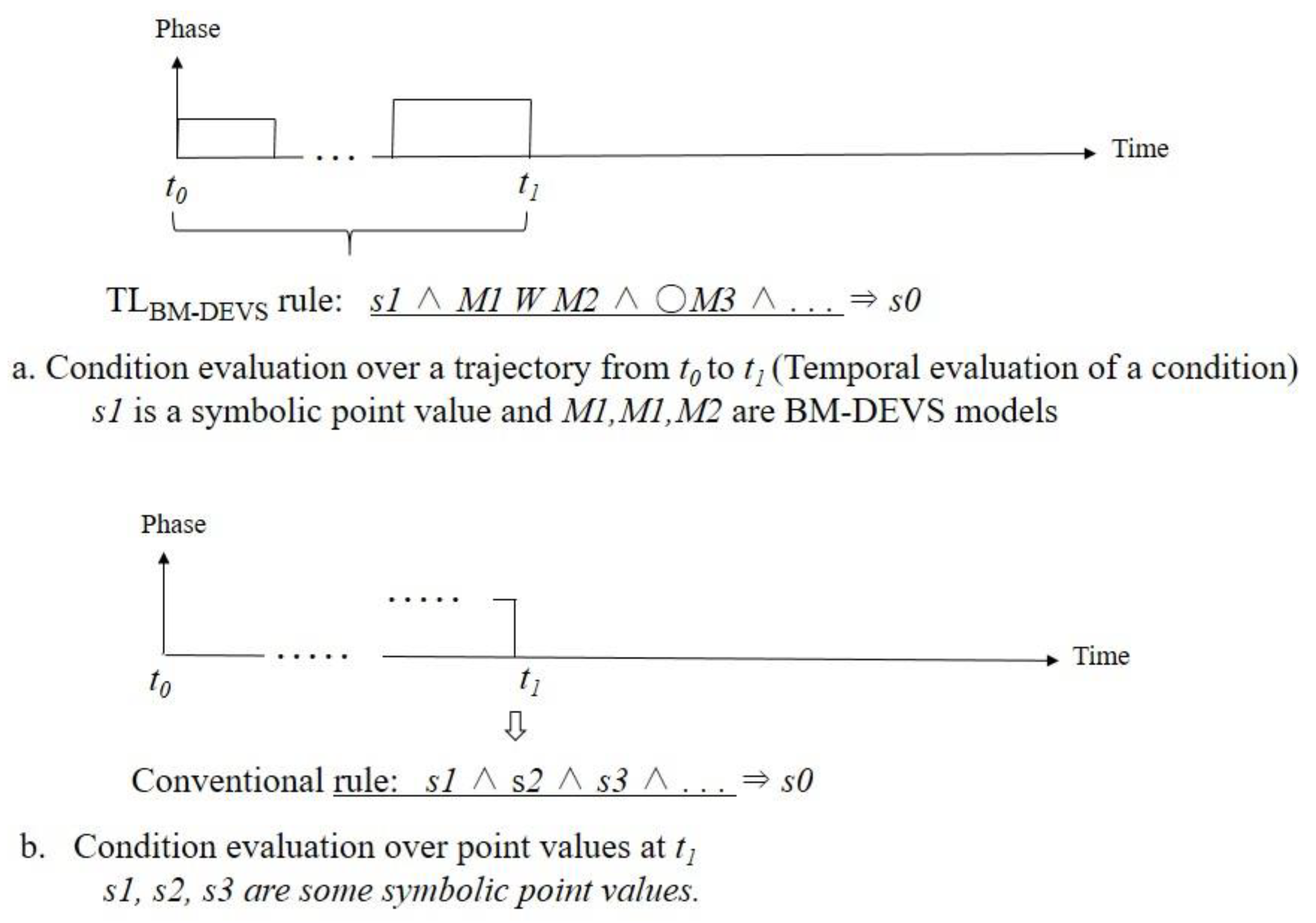
2.2. TL (Temporal Logic)

TL has been used since the 1960s and it has proven to be effective in the formal specification and verification of complex systems such as concurrent and distributed reactive systems. TL is essentially a knowledge-representation scheme in which the information for the passage of time and the temporal relationship among the arguments of the TL formulae are incorporated in the conventional logic. The major temporal operators used in TL formulae, in addition to the conventional logic connectives “not”, “or”, and “and”, are ○ for expressing the next moment, ◇ for some future moment, □ for all future times, ∪ for continuation until some future moment, and W for continuation unless some future moment [8].

Temporal formulae can also be described using the Büchi automata (BA) [12,14] with the structure

BA = (A, S, δ, I, F),

(3)

where A represents finite propositional symbols used as inputs, S is a set of sequential states, δ ⊆ Sⅹ Aⅹ S is a state transition relation, ⅹ is a cross product of sets, I ⊆ S is a set of initial states, and F ⊆ S is a set of final states.

3. BM-DEVS Formalism

Smart systems require some form of automated control for a long period of time without human intervention. To have such control, the controller should be able to track and monitor the occurrence of important behaviors within the target real system. Since the objective of implementing simulation models defined by BM-DEVS is to monitor the behavior of a target real system in real-time, the controller software can be designed and implemented by the simulation models. The behavior to be monitored is expressed as a set of temporal logic (TL) production rules, called TL_BM-DEVS rules or TL_BM-DEVS, within a multi-component model, which consists of multiple component models.

3.1. BM-DEVS Structure

In BM-DEVS, the structure for the basic models is the same as that of classic DEVS and multi-component models, or coupled models, and is defined by the structure

N_BM-DEVS = (N, P, B, Z_f,_p),

(4)

where:

N is a classic DEVS coupled model [11].

P is a set of sequential phases determined by ×P_d where P_d is a set of sequential phases of component models, and d∈ D, where D is a set of component names. The phase is the symbolic name for representing the state of a model.

B is a set of Büchi automata translated from the TL_BM-DEVS rules describing the trajectories for monitoring. A TL_BM-DEVS rule is a TL implication formula whose arguments are BM-DEVS models.

Z_f,p is a set defined by Z_f,p = {(f_b, p) | f_b∈F_b, b∈B, p∈P} ⊆ (∪_b∈B F_b) × P. That is, Z is a translator function that maps Z_f,p: F_b → P, where f_b is one of the final states (F_b) of the Büchi automata, b∈B. When the desired behavior is detected within N_BM-DEVS, a certain phase p∈ P is set by Z_f,p. Execution of Z_f,p is equivalent to firing of a rule causing a phase transition of a coupled model of N_BM-DEVS.

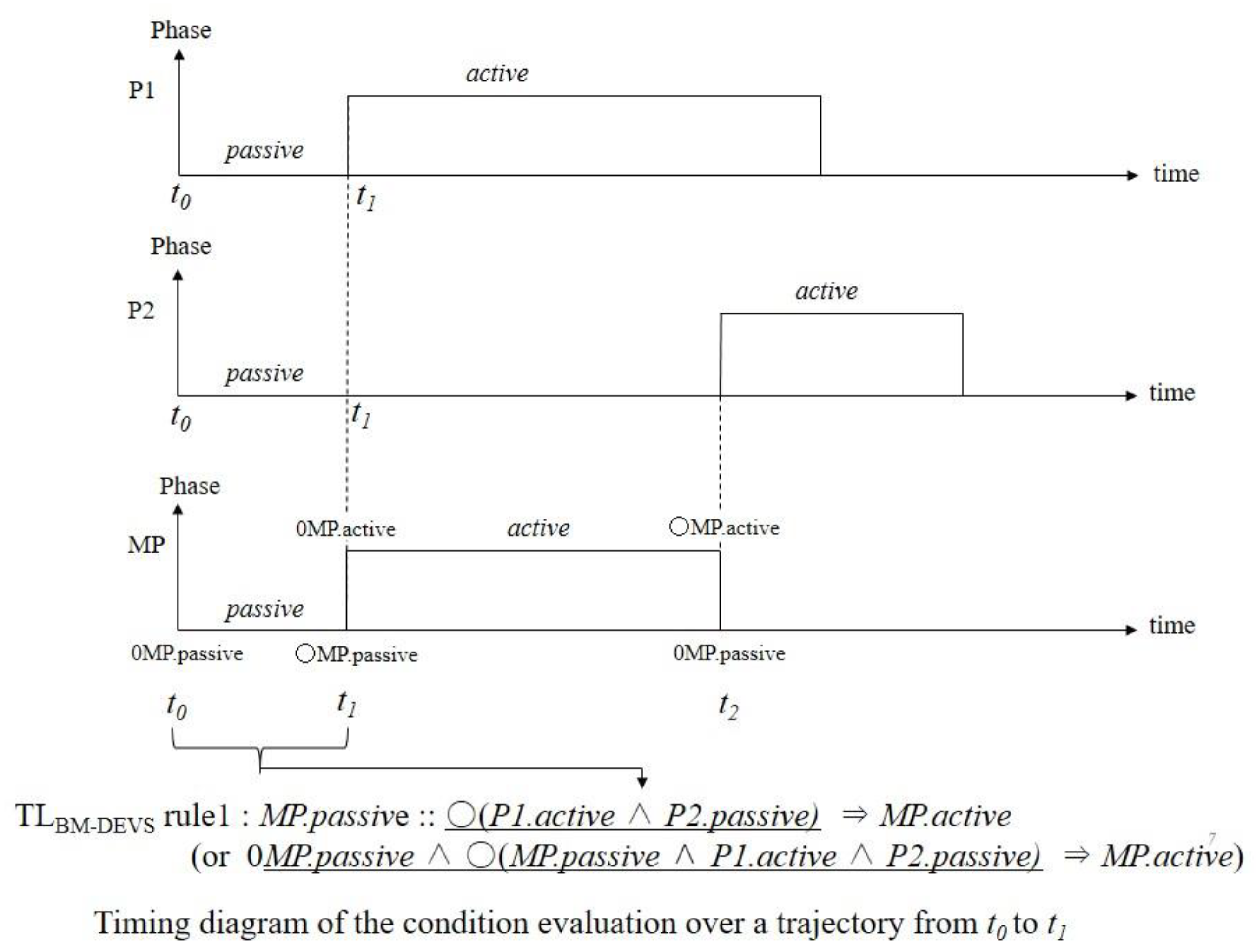
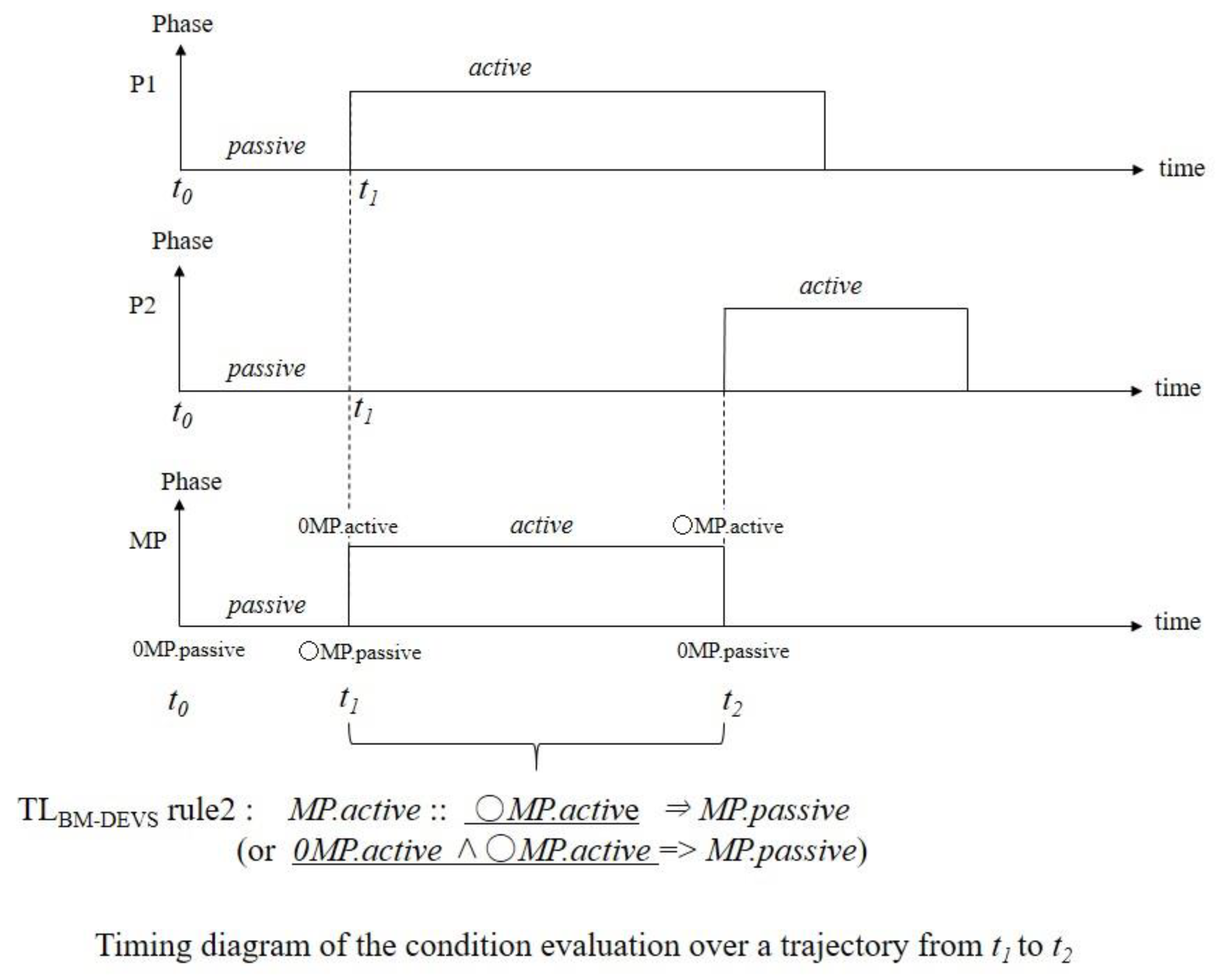
3.2. Evaluation of TL_BM-DEVS Rules

A TL_BM-DEVS rule is similar to a temporal logic implication formula whose arguments are BM-DEVS models. The condition of a TL_BM-DEVS rule is evaluated to be true when an inference engine finds that the trajectory (behavior) of the component models match the trajectory description in the conditions of the rule. One of the differences in TL_BM-DEVS from other TL is that since the time-space in BM-DEVS models is continuous as in classic DEVS models, the time-space in TL_BM-DEVS rules is also continuous, rather than discrete. We will elaborate on this issue in the discussion section.

The inference engine evaluates the condition of a TL_BM-DEVS rule based on the time-dependent behavior of the component models, rather than just based on the static point values. Such an inference engine is called an IE_BM-DEVS (Inference Engine—BM-DEVS). The IE_BM-DEVS is different from a conventional inference engine in that the rules being evaluated in the IE_BM-DEVS are TL_BM-DEVS type rules rather than the conventional point value-dependent type rules. A comparison of the condition evaluations in the two different types of rules is given in Figure 1.

Figure 1a shows the trajectory described by the condition of a TL_BM-DEVS rule. The IE_BM-DEVS evaluates the trajectory over a time period between t₀ and t₁ to determine if the behavior described in the conditions of the rule has occurred. If it has, the simulator may fire the rule after a conflict resolution and set the model to state s0. So, to evaluate the trajectory, tracking of the trajectory from t₀ until t₁ is needed. Whereas, the evaluation process of a conventional non-TL_BM-DEVS rule just checks if the point values described in the conditions of the rule are true at t₁ (Figure 1b).

3.2.1. Description of Phase Values in a Coupled Model and the Done-Messages in an IE_BM-DEVS

The done-message, done(t), of a classic DEVS abstract simulator is modified to done(p,t) in BM-DEVS abstract simulators, where p is the phase value of a component model notifying its parent simulator of its current phase, where the phase stores a symbolic name for representing the state of a model. Through this notification, the simulator of the parent model can keep track of the phases of all component models, which are needed to evaluate the TL_BM-DEVS rules assigned to a parent model or coupled model. All the done-messages from the component models’ simulators are delivered with the component models’ initial phase values to the parent simulator just once if the done-messages are the one-time initial done-messages. In the case of non-initial messages, the done(p, t) message with the smallest t value (indicating the most imminent next event time) is delivered to the parent abstract simulator, as in the classic DEVS simulator [12].

The p-value in the done(p, t) messages can have either a nil value or a non-nil value. The phase p is nil when there is no phase change in the corresponding component model, indicating that the done(nil, t) message has nothing to do with the IE_BM-DEVS part of the abstract simulator. This results in no execution of the IE_BM-DEVS and no advancement of the moment value of this phase in the parent simulator receiving the done(nil, t) message. If the phase p is non-nil, then the parent simulator receiving the done(p, t) message invokes execution of the IE_BM-DEVS part as well as the rest of the conventional part of the BM-DEVS abstract simulator, and the moment advances by one, i.e., the current-moment becomes the current-moment + ○ of the phase. Note that the moment value expressed by ○ is required by the IE_BM-DEVS only for the evaluation of TL_BM-DEVS rules, not for the conventional simulator. Note that the moment value represents the elapsed time within a phase, so that whenever there is a phase change, the moment value resets to 0.

The change of the phase value in a coupled model according to a TL_BM-DEVS rule indicates that one of the goals of the TL_BM-DEVS rules has been realized. As a result, the moment is reset to 0 in a new phase, indicating that a new goal is to be pursued. After this phase change, the new phase value is reported upward to the parent simulator of the sender coupled model in a done(p, t) message, as explained previously. Upon receipt of this done(p, t) message, the parent or receiver simulator seeks the possibility of changing its phase too. This decision depends on the rules assigned to the receiver. On the other hand, if there is no phase change in the sender, the done message done(nil, t) is sent to the parent. In this case, there is no possibility of changing the phase of the parent receiving this message since the phase change did not occur in the sender or component model, which also means that no goal has been achieved at the sender component model. As a result, no goal can be achieved at the receiver parent model.

The goal of a component model can be viewed as a subgoal from its parent’s perspective. It is obvious that if the subgoal is not achieved, the goal cannot be achieved. Thus the done(nil, t) message is not related to any of the behavior monitoring tasks of the BM-DEVS. The origin of the done message, whether the phase value is nil or not, is an atomic model that is located at the lowest level of the hierarchy. In summary, only the phase change of a model, whether it is an atomic model or a coupled model, can invoke the IE_BM-DEVS part of the BM-DEVS abstract simulator and cause a moment to advance [12].

3.2.2. Algorithm for the Inference Engine Part of the BM-DEVS Abstract Simulator

The following Algorithm 1 is the algorithmic description for the inference engine, IE_BM-DEVS, part of the BM-DEVS abstract simulator that performs TL_BM-DEVS rule evaluation. The rest of the abstract simulator is for executing the instructions in the models to carry out the simulation process [10,11].

Algorithm 1. Algorithmic description for IEBM-DEVS
1	repeat//start the abstract simulator with temporal evaluation on the TLBM-DEVS rules
2	if receive done-message(pd, t) then
2	//done-message is issued by a component model that has just gone through a phase change
4	//pd is a phase value of the component model d, t is the current simulation time
5	if pd ≠ nil then//IEBM-DEVS is invoked
6	cm = cm + ○//advance the cm (current moment) by one, initially cm = 0, ○ is the next moment
7	update {pd}//update the phase values of all the component models
8	if AB = ’() then
9	determine AB from B based on {pd} and p (or CM.p)
10	//CM.p is the phase of this model CM
11	//AB (set of active rules: a set of rules whose conditions are true up
12	to the current time point.). B a set of all the rules of this model. AB is a subset of B.
13	//true condition: the trajectory patterns in the condition of the rules
14	match that of the component models and this model
15	else
16	update every ab.s where ab∈AB
17	//make state transitions on every ab∈AB with ab::δ and {pd} and p
18	//ab::δ is a state transition function of ab
19	end if
20	if any ab.f has reached then//ab.f is a final state of ab
21	p = Zf,p//start a new phase p of this CM,
22	//Zf,p is a translation function that maps a final state of rule ab to a CM’s phase
23	set AB = ’( )
24	cm = 0
25	end if
26	end if //end of if pd ≠ nil
27	{
28	…
29	//Same as the execution of a classic DEVS abstract simulator part w/o the
30	IEBM-DEVS involved.
31	//Executed for both done(p, t) and done(nil, t) cases. The classic DEVS
32	abstract simulator does not distinguish between these two done messages.
33	…
34	}
35	if p changed then
36	return done(p, t)//return the phase of this CM to the higher level abstract
37	simulator, which makes the parent of this CM advance
38	the current moment ○ by one
39	else
40	return done(nil, t)
41	end if
42	end if//end of if receive done-message(p, t)
43	until the end of the simulation//end repeat

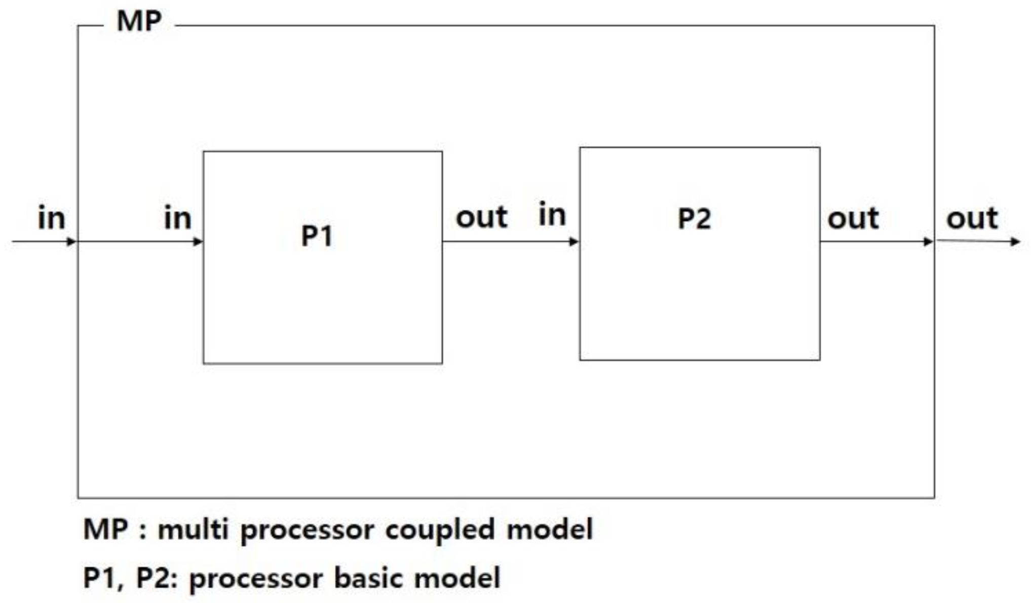
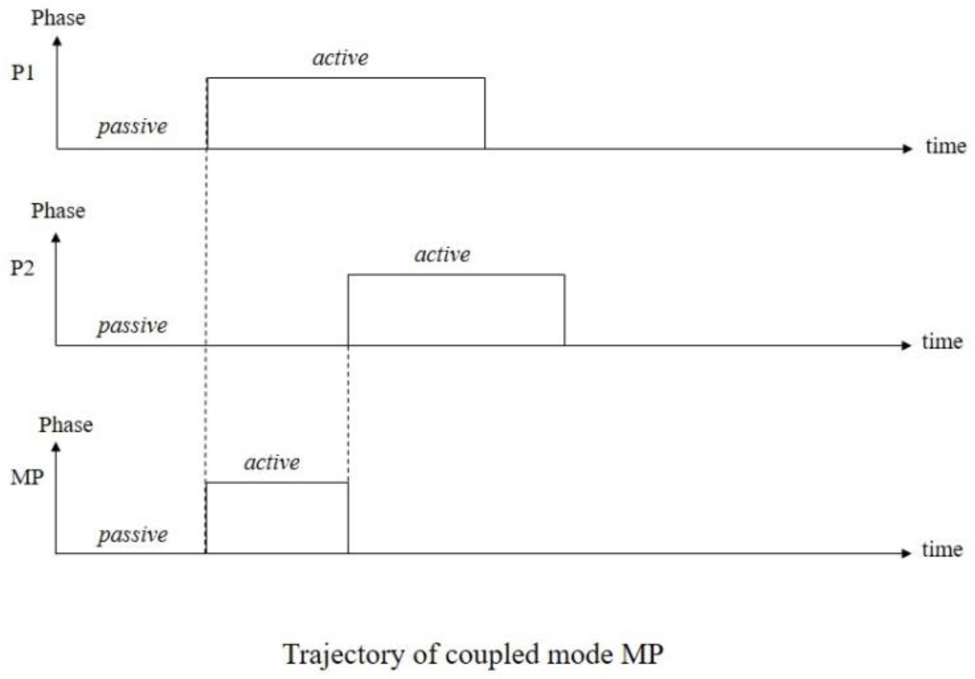
4. Simple Modeling and Simulation Example of the BM-DEVS

This section shows how a simple coupled model, or multi-component model, can be defined according to BM-DEVS formalism as an example to show the correctness of this formalism in Section 4.1. This section also illustrates how the IE_BM-DEVS part of the BM-DEVS abstract simulator performs in the example in Section 4.2.

4.1. BM-DEVS Model Specification Example

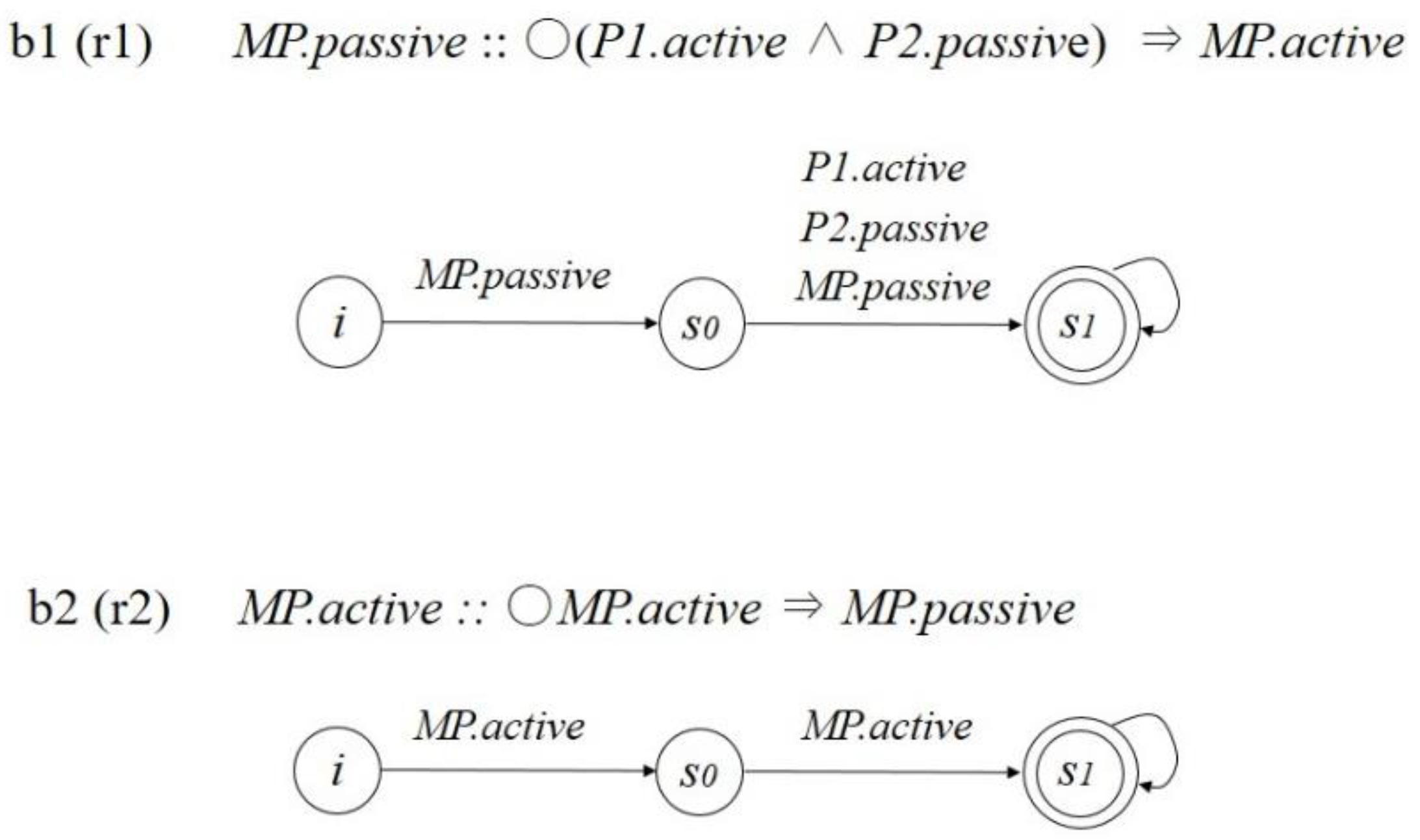
The Multi-Processor (MP) model shown in Figure 2 is a coupled model composed of two-component models P1 and P2.

The trajectory pattern that the MP wants to monitor is shown in Figure 3. The MP monitors and transits from “passive” to “active” once the transition of P1 from “passive” to “active” occurs, as expressed in Rule 1. The MP transits from “active” to “passive” at the next moment when P2 transits from “passive” to “active”, as expressed in rule 2. The MP changes phases whenever the trajectory patterns it wants to monitor are detected, as expressed in the rules. In Rule 2, the MP changes phase from “active” to “passive” at the next moment during phase MP.active, regardless of which component model determined the next moment’s actual time or sent the done-message. The phase name of the MP reflects the symbolic meaning of the trajectory it has just detected. This desired trajectory pattern being monitored is expressed via two TL_BM-DEVS rules as shown below.

Rule 1.

MP.passive :: ○(P1.active ∧ P2.passive) ⇒ MP.active

//If MP.passive at the initial moment and at the next-moment P1.passive and P2.passive, then transit to MP.active.

Rule 2.

MP.active :: ○MP.active ⇒ MP.passive

//If MP.active at the initial moment and at the next-moment MP.active, than transit to MP.passive.

The coupled BM-DEVS specification of the MP model is

N_BM-DEVS = (N, P, B, Z_f,_p)

(5)

where:

N is the classic DEVS multi-component model;

P = {passive, active};

B = {b1, b2}; //b1, b2 are a Büchi automata representation of TL_BM-DEVS Rule 1and Rule 2, respectively;

Z_f,p = {(b1.s1, MP.active), (b2.s1, MP.passive)}.

TL_BM-DEVS Rules 1 and 2 are shown in Figure 4 is a pictorial representation of Büchi automata [12,15] b1 and b2, respectively. The state transition diagrams below show how the transitions are made. Initially, all the automata are at state i, which indicates that they are de-activated. Once activated, these automata enter state s0 from i. The double circle in the figure represents the final state, indicating that the trajectory expressed in the conditions of a rule has been generated; as a result, a phase change at the current model occurs.

Once any of the rules reaches a final state, all the active rules are de-activated for the next tracking of the components’ trajectories. Any further tracking should be made based on the new phase just entered, as in the DEVS models’ state transitions for state trajectory generation, where the next phase is entered sequentially one after another. If there are more rules still active by the time a rule reaches a final state, the conflict resolution strategy should determine whether to keep tracking or to stop tracking to make a phase change of the model immediately, which results in the de-activation of all the rules.

The TL_BM-DEVS Rules r1 and r2 shown in Figure 4 are represented by the Büchi automaton [12] b1 and b2, respectively, as shown below.

Büchi automaton is defined by B = (A, S, δ, I, F)

Where, for automaton b1:

A = P({MP.passive, MP.active}°{ε, P1.passive, P1.active}°{ε, P2.passive, P2.active});

S = {i, s0, s1};

δ = {(i, MP.passive, s0), (s0, MP.passive P1.active P2.passive, s1)};

I = {i};

F = {s1};

And for automaton b2:

A = P({MP.passive, MP.active}°{ε, P1.passive, P1.active}°{ε, P2.passive, P2.active});

S = {i, s0, s1};

δ = {(i, MP.active, s0), (s0, MP.active, s1)};

I = {i};

F = {s1}.//Z_f,p translates s1 into passive or MP.passive.

4.2. BM-DEVS Abstract Simulator Example

This section shows how the inference engine part, IE_BM-DEVS, of the BM-DEVS abstract simulator is executed to monitor the trajectories of component models P1 and P2, which are arguments of the TL_BM-DEVS rules stored in the coupled model MP. The simulator is being executed while the MP transits from passive to active and returns to passive. Since these transitions occur according to the trajectories of P1 and P2, the transitions of the trajectory of the MP are the result of monitoring the MP on the component models.

Figure 5 and Figure 6 show the timing diagrams of the trajectories of P1, P2, and the MP. The trajectory of the MP is determined by that of P1, P2, rule 1, and rule 2 (Figure 4). Thus, the trajectory of the MP depends on how the trajectories of P1 and P2 are interpreted according to the rules. That is, for the same set of trajectories of P1 and P2, the trajectory of MP can be different depending on how the trajectory is interpreted by the rules. The current moment and the next moment are expressed by the symbols 0 and ○ followed by the phase values, e.g., 0P1.active… or ○P2.passive…, etc. Whenever the phase change occurs, the initial moment 0 is the new phase’s current moment, that is, whenever the MP makes a phase change, the moment resets to 0, or the initial moment. So the moment 0 can be incremented to ○, ○○, ○○○, … as long as the phase is unchanged. Note that the actual simulation time for the first moment 0 of a phase is different from that of the second moment 0 of the same phase. This difference is identical to what happens in classic DEVS [10], except that there is no moment value attached to a certain phase when it is entered.

In Figure 5, the monitoring of the trajectory expressed in the condition of Rule 1 spans from t₀ to t₁, or from 0MP.passive to ○MP.passive. At ○MP.passive, the MP model transits to the “active” phase since the trajectory expressed in the condition formula of Rule 1, MP.passive :: ○(P1.active ∧ P2.passive), is detected, as shown in the timing diagram. Thus, the time point changes to 0MP.active, which is identical to ○MP.passive at that time point.

The detection of the trajectory and transition just described corresponds to executions of the abstract simulator up to step3, where step1 (refer to Execution steps in the abstract simulator of BM-DEVS below) just shows the initial values of the simulator and step2 shows how the simulator executes once all the initial one-time done-messages are received at 0MP.passive or t₀. Note that in step2, b₁ (Büchi automaton, representing Rule 1) becomes active, indicating that the simulator begins monitoring to detect the desired trajectory expressed in the conditions of Rule 1. In step3, when done(p1.active) is received, the simulator is able to detect the desired trajectory, and as a result of the detection, b1 transits from b1.s0 to b1.s1, where b1.s1 is the final state of b1, which is equivalent to MP.active. This equivalence is found by the translator function Z that translates a Büchi automaton state to an MP phase. Due to the phase change to “active”, the new time point begins with 0, or the time point resets to 0. At this moment, all the active automata in B are deactivated and re-evaluated. As a result, b₂ transits to b₂.s0 from b₂.i, indicating that b₂ became active; thus, the monitoring on b₂ begins, as shown in step3.

The description in Figure 6 is similar to that of Figure 5. In Figure 6, the monitoring of the trajectory expressed in the conditions of Rule 2 spans from t₁ to t₂, or from 0MP.active to ○MP.active. At ○MP.active, the MP model transits to the “passive” phase since the trajectory expressed in the condition formula of Rule 2, MP.active :: ○MP.active, is detected, as shown in the timing diagram. Thus, the time point changes to 0MP.passive, which is identical to ○MP.active at that time point. The detection of the trajectory and transition just described corresponds to executions of the abstract simulator from step 3 to step 4.

As mentioned previously, b2 became active by transiting to b2.s0 in step3. In step4, when the done(p2.active) message is received, the simulator is able to detect the desired trajectory expressed in the conditions of Rule 2, and as a result b2 transits from b2.s0 to b2.s1, where b2.s1 is the final state of b2, which is equivalent to MP.passive. This equivalence is found by the translator function Z as before. Due to the phase change to “passive”, the time point resets to 0. At this moment, all the active automata in B are deactivated and re-evaluated. As a result, none are activated and the active set AB becomes empty. This cycle continues until the end of the simulation.

Execution steps in the abstract simulator C:MP of BM-DEVS
1	[Step 1]
2	Initial values of C:MP—the values before the one-time initial done-messages are
3	received//C:MP is the abstract simulator for the MP model
4	{pd} = ’( )//initial phase values of the component models
5	p = passive//phase of the MP, passive initially otherwise specified
6	B = {b1.i, b2.i}//set B shows all the members of B with the current state values
7	AB = ’()//initially none of the automata (rules) of δ activate for b∈B, i.e., b1 and b2
8	B’ = {b1.i, b2.i}//set B after execution of δ
9	Zf,p = {(b1.s1, MP.active), (b2.s1, MP.passive)}//the final state of b1.s1 is identical
10	to the MP’s active state
11	[Step 2]
12	At time 0MP.passive—at initialization time, when initial messages
13	done(p1.passive, t) and done(p2.passive, t) are received
14	{pd} = {p1.passive, p2.passive}
15	p = passive
16	B = {b1.i, b2.i}//set B shows all the members of B with the current state value
17	AB = {b1.s0}
18	B’ = {b1.s0, b2.i}//after execution of δ
19	Zf,p (b1.s0) => ’()//no change of the MP’s phase because b1.s0 is not a final state
20	[Step 3]
21	At time ○MP.passive—when done(p1.active, t) is received
22	{pd} = {p1.active, p2.passive}
23	p = passive
24	B = {b1.s0, b2.i}
25	AB = {b1.s1}//b1 reached at the accepting state or final state
26	B’ = {b1.s1, b2.i}
27	Zf,p (b1.s1) => active
28	//after executing Z and clearing AB and selecting AB from B
29	//at time 0MP.active same as ○MP.passive
30	{pd} = {p1.active, p2.passive}
31	p = active
32	B = {b1.i, b2.i}
33	AB = {b2.s0}
34	B’ = {b1.i, b2.s0}
35	[Step 4]
36	At time ○MP.active—when done(p2.active, t) is received
37	{pd} = {p1.active, p2.active}
38	p = active
39	B = {b1.i, b2.s0}
40	AB = {b2.s1}
41	B’ = {b1.i, b2.s1}
42	Zf,p (b2.s1) => passive
43	//after executing Z and clearing AB and selecting AB from B
44	{pd} = {p1.active, p2.active}
45	P = passive
46	B = {b1.i, b2.i}
47	AB = ‘()
48	B’ = {b1.i, b2.i}
49	Steps continue until the end of the simulation.

4.3. Context-Aware Architecture Implementation as a BM-DEVS Application

To be fully aware of the context of an environment or a target system, the behavior of the events in concern within the system should be monitored by keeping track of the event trajectories in the system, instead of just acquiring the point data values. One way to acquire these non-temporal point data values from the target system for context-awareness by exploiting the simulation models is proposed in [9]. Since the simulation models implemented based on BM-DEVS are aimed at monitoring the behavior of component models, the behavior of the target real system can also be monitored indirectly by connecting the system to the system models, which replicates the behavior of the target system, through sensors or networks. Through this behavior monitoring on the models, context-awareness of the models can be achieved, through which the context-awareness on the connected target system can be achieved.

The phase of a BM-DEVS coupled model can be interpreted as a context for the component models. For example, if the phase is “battle”, then a firing event is considered to be something normal, whereas, if the phase is “peace”, then the same firing event is an abnormal event that requires immediate scrutiny. So, if the phase of the parent coupled model is used to express a context, then the component model’s behavior is interpreted depending on the phase value.

Figure 7 shows a simplified composition of a context-aware architecture (CAA) and a real-world system, whose context-awareness is achieved by the CAA. Internally, the CAA contains the simulation models, the structure of which is identical to the real-world system, so that the behavior of the simulation model can replicate the behavior of the real system. The simulation models object_1, …, object_n are BM-DEVS models through which monitoring of the real-world system is possible.

5. Discussion on BM-DEVS

The main purpose of BM-DEVS is to give the behavior monitoring capability to coupled models by keeping track of the trajectories of the component models. This purpose is achieved by exploiting the existing theories such as the DEVS formalism, its abstract simulator, temporal logic system, and inference engine, as explained in previous sections. That is, in defining BM-DEVS, the additional elements P, B, and Z_f,p are added to classic DEVS, and the abstract simulator is modified to allow the execution of these new elements. Additionally, the proposed inference engine IE_BM-DEVS is added to the abstract simulator. Regarding the temporal logic, the major modification is to allow DEVS models to be the arguments in a TL rule, which in turn results in changing the view of the flow of time from discrete time-space to continuous time-space, since DEVS is defined based on continuous time-space. Naturally, the inference engine that executes the rules is modified to accommodate these changes, as explained in Section 3.2.

5.1. Efficiency of BM-DEVS for Behavior Monitoring

Without BM-DEVS, the behavior of component models can be monitored by adding an extra component model whose major role is to collect the trajectory information of the other component models and let the extra model detect the behavior. This approach is similar to having an extra model for delivering the inputs and the outputs among other components without using the input-output coupling information in a DEVS coupled model. The modeling efficiency between the former and the latter approach is huge if the purpose is just to monitor the behavior. In short, most of the modeling efforts for behavior monitoring are implemented in the proposed abstract simulator. Besides, there is added computation overhead for the extra model to collect all the trajectory information from the component models that are being monitored, which cause executions of external transitions, internal transitions, and output functions of the involved models too frequently.

If the desired behavior to be monitored is expressed as rules, modifying the desired behavior to be monitored is simply achieved by modifying the rules, rather than modifying the model codes, which requires much more time and effort. Since those rules form a rule base, which is a modularized knowledge base separated from the rest of the model codes, where and what to modify can be easily identified as well. Once a knowledge base is formed, there are many advantages, such as easy addition, deletion, and modification of the knowledge without worrying about undesired side effects on the other parts of the model codes. Further, semantically, the content of the knowledge can be easily understood because other irrelevant operations are totally separated from the knowledge base. There is a subclass of atomic models called forward models [10] in which a set of non-temporal production rules are used to express the complex relationship of state changes and input-output handling. However, this type of model is not used for monitoring behavior as in BM-DEVS models.

5.2. Determination of the Moment Value and Its Duration

The moment value used in a BM-DEVS model is equivalent to the elapsed time in a certain phase, the purpose of which is to match the condition of the temporal logic rule to the component models trajectory to cause a phase transition. In a DEVS model, only the phase value is used since the purpose is not trajectory monitoring.

The next moment within a phase is determined by the next-event-times of the children component models, and the component next moment is determined by its component models, and so on until this repetition continues down to the bottom level component models, called atomic models. Among immediate component models, the next moment, ○, of a coupled model is determined by the component model that has just gone through a phase change. This is the model that has just sent the new phase value in a done-message done(p, t) to the parent coupled model. Upon receipt of the message, the coupled model may go through a phase change depending on the conditions of the rules assigned to the model. If the coupled model changes the phase, the current moment is reset to 0 after entering into a new phase, otherwise, the current moment advances by one moment, i.e., the current-moment becomes the current-moment + ○ within the same phase. Thus, depending on how rules are formulated among the coupled models, the current moment value of a phase for different models is determined differently, and the difference in the time point when the done-message is received also affects the moment value.

Since the moment is defined in continuous-time rather than discrete-time, the duration of each current moment is likely to be different. The duration is determined by the rules and done messages, as explained in previous sections. The interesting matter is that the duration of a moment tends to get longer as we go up along the hierarchy of the models, since even if a component model changes the phase, the parent model may not change the phase, resulting in no advancement of the moment value; this ultimately leads to longer duration of the current moment. The time limit on the next moment can be imposed globally on all models identically or locally on each model differently as needed.

5.3. Comparison with Other Context-Awareness Approaches

Many context-aware architectures of various purposes acquire context data in the form of point values from the environment to adapt systems behavior accordingly [3,4,16,17]. Thus, acquired context data become inputs to the architectures. For example, [8] presents a textual domain-specific language that models context information to automatically generate software artifacts from context models. In the overall process, the general perception of behaviors that are expressed based on both temporal and spatial values is not considered.

Since the end purpose of the context-aware architectures can be summarized as the detection of certain behaviors of interest, the environment or inputs to the architectures should be expressed in a form of behavioral patterns rather than just point values. Some context-aware architectures showed how the behavioral patterns can be structured internally from various values including the input point values and used the related structured patterns for detecting the desired behaviors [5,6,18]. The structures are, however, not for expressing input behavioral patterns nor domain-independent representations based on coherent general methodologies.

The study [7] proposes a logical-based framework to recognize and analyze behavioral specifications as a formal logic language and automatically discovers behaviors from sensory data streams. The research [19] presents a logical framework for modeling and verifying context-aware multi-agent systems. Both of the researches represent the knowledge about environment behaviors using temporal logic. The temporal logic is, however, often not suitable for modeling behavior of real-life complex systems since it lacks the expressive power of the structural knowledge.

To accurately detect the behavior of interest, there should be a way to express and store the real-world behavioral patterns so that the stored patterns can be used as inputs for the context-awareness. Since the main purpose of simulation models is to express and store the behavior of the real-world system of concern, the simulation models are used as inputs in the proposed context-aware architecture design. The BM-DEVS methodology shows how the behavioral knowledge stored within the models can be exploited for the detection of the desired behavioral patterns.

The paper [20] showed how to formalize system requirements based on the context-aware probabilistic temporal logic with the target system being modeled as an MDP. The main content of the paper is composed of the details of requirement specifications as the objectives, as well as how to achieve these goals. Whereas the proposed paper’s main contribution is in (1) how to represent the desired behavior to monitor and (2) how to monitor and detect this behavior. The desired behavior is represented as a state trajectory expressed by TL_BM-DEVS, which is a temporal logic whose arguments are BM-DEVS simulation models, as shown in Figure 3. Note that the state trajectory of this type can represent any behavioral pattern irrespective of its purpose.

Among a virtually unlimited number of possible behavioral patterns or state trajectories dispersed in the simulation model of a real complex system, the BM-DEVS model should be able to monitor and detect the occurrence of the desired state trajectory pattern by tracing all the state transitions of component models. Since the state transitions of the models have to be traced, the arguments of the temporal logic (TL_BM-DEVS) naturally become the simulation models, which also results in the need for designing a temporal inference engine (IE_BM-DEVS) capable of tracing the state transitions of the models for a certain interval of time, as shown in Figure 1. The inference engine reasons are based on a set of model states that correspond to either an initial state, an intermediate inferred state, or a goal state.

The main limitation of [9] is the lack of proper methodology for expressing the desired behavior and monitoring the behavior. In that paper, the desired behavior to monitor is expressed by a heuristic algorithm, and monitoring of the behavior is performed by tracing through the state transition patterns according to the algorithm. This limitation can be described as that of the conventional software system compared to the knowledge-based system.

5.4. Verification of the Validity of BM-DEVS

This paper verifies the proposed methodology in two directions. First, how the desired behavior can be monitored is explained and verified according to the following orders. Once the definition of the proposed methodology is given as in Section 3.1, the principle of how the methodology can monitor the behavior is described as in Section 3.2. The Section 3.2.1 and Section 3.2.2 explain in detail the monitoring process by showing the pseudo level algorithm. The example in Section 4 shows how a BM-DEVS model is constructed and how monitoring of the desired behavior is actually achieved. Second, the effectiveness and validity of the proposed methodology can be verified by the following statement. The BM-DEVS simulation model replicates the behavior and structure of real-world systems. Within the model, the behavior of the real systems is represented by state trajectories. Once the behavior is represented in the form of a state trajectory, the BM-DEVS model can monitor the trajectory, as verified by the first statement above.

How well the BM-DEVS simulation model can replicate the behavior of the real-world system is an issue of validity (how correctly the behavior can be replicated) and fidelity (how detailed the behavior can be replicated) of the classic DEVS formalism [10,11], which is theoretically sound and widely accepted by simulation practitioners. Verification through solving a real-life complex system is the subject of a subsequent research paper.

6. Conclusions and Future Work

All activities that occur in the real-world are based on two factors, time-space and state-space. Thus, to accurately express and recognize the dynamics of the activities, these two factors must be considered. To build any type of autonomous smart system, the behavior monitoring of the activities of concern, which are expressed and recognized based on both time-space and state-space, is indispensable. The simulation models can be built to replicate the behavior of the real-world system of interest. By monitoring such models defined by BM-DEVS, we can indirectly yet accurately monitor the system.

The proposed paper’s main contributions are, first, how to represent the desired behavior to be monitored and, second, how to monitor this behavior. The desired behavior is represented as a state trajectory expressed by TL_BM-DEVS, which is a temporal logic whose arguments are BM-DEVS simulation models, as shown in Figure 3. Note that the state trajectory of this type can represent any behavioral pattern irrespective of its purpose as long as the pattern can be generated within the models. To monitor the state trajectories of interest among a virtually unlimited number of possible trajectory patterns dispersed in the simulation model, a methodology that defines the components and their roles for monitoring the task is essential, as proposed in this research. According to the proposed methodology, since the state transitions of the models have to be traced, the arguments of the temporal logic (TL_BM-DEVS) naturally become the simulation models. The simulation models as arguments of the rule, in turn, result in the need for designing a temporal inference engine (IE_BM-DEVS) capable of tracing the state transitions of the simulation models for a certain interval of time, as shown in Figure 1.

The motivation of the proposed methodology, BM-DEVS, is based on the fact that in order to solve problems better, they should be expressed accurately to begin with. Since it is the behavior that is to be monitored in the methodology, the problems should be expressed by variables capable of capturing and storing the behavioral knowledge as well as the structural knowledge of the problems. That is, the expression of the problems within the software should be accomplished using the same fabricating factors of time and space, symmetrically to that of the real-world. The conventional data structures of graphs, trees, etc. lack the ability to express the temporal aspects of the problems, which is essential for expressing the overall behavior; similarly, temporal logic lacks the ability to express the structural aspects of the problems, which is essential for expressing complex problems in the real-world. The simulation models are efficient in both regards [10,11]. These simulation models are used as arguments of the proposed temporal logic type TL_BM-DEVS.

The arguments are variables pointing to behavioral data structures composed of simulation models. These models should be defined based on the BM-DEVS formalism to be able to store TL_BM-DEVS rules and monitor trajectories expressed by the rules. The rules are executed by the proposed inference engine IE_BM-DEVS and the algorithm for the inference engine is shown in Section 3.2.2. Note that the behavioral knowledge is stored via variables in this research. Further, since these variables are among the most basic factors constituting a problem solver, how the variables are defined affects all the subsequent designs, such as compound data structures, various levels of functions, and problem-solving algorithms, all of which determine whether problems can be expressed accurately and solved correctly.

Solving problems based on both time-space and state-space properties is achieved through the BM-DEVS formalism for behavior monitoring of simulation models. Future research will be focused on developing more formalisms for various purposes based on simulation theory and AI. The former is efficient in solving time-related problems, and the latter is efficient in solving problems in which time is less involved. An application of solving a real-life complex system is the subject of a future research paper. While working on this subject, a generic variable type capable of storing behavioral knowledge as arguments for various algorithms will be studied rather than simply adopting the simulation model in the current form specified by [10,11] as the arguments. This study requires a formal approach to defining a variable type and exploiting the variable.

Currently, the temporal logic is exploited to formulate the condition of a TL_BM-DEVS rule to monitor the trajectories of the component models. However, in the future, temporal logic will be applied to the action of the rule as well. In this case, the action to be executed is expressed by the temporal logic formula, i.e., the action expressed in a TL_BM-DEVS rule becomes a goal to be achieved. RG-DEVS (goal ReGression DEVS) [21] can be extended to implement the simulation model to achieve the goal expressed in a TL_BM-DEVS rule, and the model thus implemented becomes the controller software module for a real-world system under control.

References

1. Jamil, M.S.; Jamil, M.A.; Mazhar, A.; Ikram, A. Ahmed, Smart environment monitoring system by employing wireless sensor networks on vehicles for pollution free smart cities. Procedia Eng. 2015, 107, 480–484. [Google Scholar] [CrossRef] [Green Version]
2. Rashid, B.; Rehmani, M.H. Applications of wireless sensor networks for urban areas: A survey. J. Netw. Comput. Appl. 2016, 60, 192–219. [Google Scholar] [CrossRef]
3. Vahdat-Nejad, H.; Ramazani, A.; Mohammadi, T.; Mansoor, W. A survey on context-aware vehicular network applications. Elsevier Veh. Commun. 2016, 3, 43–57. [Google Scholar] [CrossRef]
4. Baldauf, M. A survey on context-aware systems. Int. J. Ad Hoc Ubiquitous Comput. 2007, 2, 263–277. [Google Scholar] [CrossRef] [Green Version]
5. Fang, Q.; Xu, C.; Hossain, M.S.; Muhammad, G. STCAPLRS A spatial-temporal context-aware personalized location recommendation system. ACM Trans. Intell. Syst. Technol. 2016, 7, 59. [Google Scholar] [CrossRef]
6. Liu, Z.L.; Liu, Q.; Xu, W.; Liu, Z.; Zhou, Z.; Chen, J. Deep learning-based human motion prediction considering context awareness for human-robot collaboration in manufacturing. Procedia CIRP 2019, 83, 272–278. [Google Scholar] [CrossRef]
7. Klimek, R. Behavior recognition and analysis in smart environments for context-aware applications. In Proceedings of the IEEE International Conference on Systems, Man, and Cyberrnetics, Hong Kong, China, 9–12 October 2015. [Google Scholar]
8. Hoyos, J.R.; García-Molina, J.; Botía, J.A. A domain-specific language for context modeling in context-aware systems. J. Syst. Softw. 2013, 86, 2890–2905. [Google Scholar]
9. Nam, S.M.; Cho, T.H. Context-aware architecture for probabilistic voting-based filtering scheme in sensor networks. IEEE Trans. Mob. Comput. 2017, 16, 2751–2763. [Google Scholar] [CrossRef]
10. Zeigler, B.P. Object-Oriented Simulation with Hierarchical, Modular Models: Intelligent Agents and Endomorphic Systems; Academic Press: San Diego, CA, USA, 1990; pp. 41–143. [Google Scholar]
11. Zeigler, B.P.; Preahofer, H.; Kim, T.G. Theory of Modeling and Simulation; Academic Press: San Diego, CA, USA, 2000; pp. 75–123. [Google Scholar]
12. Fisher, M. An Introduction to Practical Formal Methods Using Temporal Logic; John Wiley & Sons: Hoboken, NJ, USA, 2011; pp. 12–48. [Google Scholar]
13. Manna, Z.; Pnueli, A. The Temporal Logic of Reactive and Concurrent Systems: Specification; Springer Science & Business Media: Berlin, Germany, 2012. [Google Scholar]
14. Sickert, S.; Esparza, J.; Jaax, S.; Křetínský, J. Limit-deterministic büchi automata for linear temporal logic. In Proceedings of the International Conference on Computer Aided Verification, Toronto, ON, Canada, 17–23 July 2016. [Google Scholar] [CrossRef]
15. Büchi, J.R. The Collected Works of J. Richard Büchi; Springer Science & Business Media: Berlin, Germany, 2012. [Google Scholar]
16. Sezer, O.B.; Dogdu, E.; Ozbayoglu, A.M. Context-aware computing, learning, and big data in internet of things: A survey. IEEE Internet Things J. 2018, 5, 1–28. [Google Scholar] [CrossRef]
17. Mueller, M.; Smith, N.; Ghanem, B. Context-aware correlation filter tracking. In Proceedings of the IEEE Conference on Computer Vision and Pattern Recognition, Honolulu, HI, USA, 21–26 July 2017. [Google Scholar]
18. Liu, N.N.; He, L.; Zhao, M. Social temporal collaborative ranking for context aware movie recommendation. ACM Trans. Intell. Syst. Technol. 2013, 4, 15. [Google Scholar] [CrossRef]
19. Cho, T.H. Embedding intelligent planning capability to DEVS models by goal regression method. Simulation 2002, 78, 716–730. [Google Scholar] [CrossRef]
20. Rakib, A.; Haque, H.M.U.; Faruqui, R.U. A temporal description logic for resource-bounded rule-based context-aware agents. In Proceedings of the International Conference on Context-Aware Systems and Applications, Phu Quoc Island, Vietnam, 25–26 November 2013. [Google Scholar]
21. Elfar, M.; Wang, W.; Pajic, M. Context-aware temporal logic for probabilistic systems. arXiv 2007, arXiv:2007.0579. [Google Scholar]
Figure 1. IEBM-DEVS: inference engine for TLBM-DEVS rules.
Symmetry 12 01568 g001
Figure 2. Multi-processor coupled model.
Symmetry 12 01568 g002
Figure 3. The trajectory pattern of the Multi-Processor (MP) to be monitored (This pattern is the result of the P1 and P2 trajectories).
Symmetry 12 01568 g003
Figure 4. Pictorial representation of TLBM-DEVS rule 1 and rule 2 shown as Büchi automata b1 and b2, respectively.
Symmetry 12 01568 g004
Figure 5. The timing diagrams of the trajectories of P1, P2, and MP for rule 1 evaluation.
Symmetry 12 01568 g005
Figure 6. The timing diagrams of the trajectories of P1, P2, and MP for rule 2 evaluation.
Symmetry 12 01568 g006
Figure 7. Context-aware architecture implemented by a simulation model.
Symmetry 12 01568 g007