Article

Low-Light Image Enhancement Based on Quasi-Symmetric Correction Functions by Fusion

1
College of Computer and Information, Hohai University, Nanjing 211100, China
2
College of Engineering, Shantou University, Shantou 515063, China
*
Author to whom correspondence should be addressed.
These authors contributed equally to this work.
Symmetry 2020, 12(9), 1561; https://doi.org/10.3390/sym12091561
Submission received: 20 August 2020 / Revised: 15 September 2020 / Accepted: 17 September 2020 / Published: 21 September 2020
(This article belongs to the Section Computer)

Abstract

:
Sometimes it is very difficult to obtain high-quality images because of the limitations of image-capturing devices and the environment. Gamma correction (GC) is widely used for image enhancement. However, traditional GC perhaps cannot preserve image details and may even reduce local contrast within high-illuminance regions. Therefore, we first define two couples of quasi-symmetric correction functions (QCFs) to solve these problems. Moreover, we propose a novel low-light image enhancement method based on proposed QCFs by fusion, which combines a globally-enhanced image by QCFs and a locally-enhanced image by contrast-limited adaptive histogram equalization (CLAHE). A large number of experimental results showed that our method could significantly enhance the detail and improve the contrast of low-light images. Our method also has a better performance than other state-of-the-art methods in both subjective and objective assessments.

1. Introduction

High-quality images have found many applications in multimedia and computer vision applications [1,2]. However, due to the limitations of image acquisition technology, imaging environment, and other factors, it is sometimes very difficult to obtain high-quality images and it is almost impossible to obtain images with low illuminance all the time. Images taken under extreme weather conditions, underwater or at night often have low-visibility and blurred details, and their quality is greatly degraded. Therefore, it is necessary to enhance low-light images in order to satisfy our demand. Researchers from academia and industry have been working on various image-processing technologies. Many image enhancement methods have been proposed to enhance the degraded images in daily life, such as underwater images [3], foggy images [4], and nighttime images [5]. In modern industrial production areas, these techniques have also found more and more applications. In [6], a novel optical defect detection and classification system is proposed for real-time inspection. In [7], a novel defect extraction and classification scheme for mobile phone screens, based on machine vision, is proposed. Another interesting application is the surface quality inspection of transparent parts [8].
Existing approaches generally fall into two major categories—global enhancement methods and local enhancement methods. Global enhancement methods aim to process all image pixels in the same way, regardless of spatial distribution. Global enhancement methods, which are based on logarithm [9], power-law [10], or gamma correction [11], are commonly used for low-quality images. However, sometimes these methods cannot output desired and gratifying results. Histogram equalization (HE) [12] is a great way to improve the contrast of the input image by adjusting pixel values according to the cumulative distribution function. However, it may lead to over-enhancement in some regions with low contrast. To overcome this defect, in [13] an enhancement method is proposed using layered difference representation (LDR) of 2D histograms, but the enhanced image looks a bit dark. Traditional gamma correction (GC) [14] maps all pixels by a power exponent function, but sometimes this causes over-correction for the bright regions.
Local enhancement methods take the spatial distribution of pixels into account and usually have a better effect. Adaptive histogram equalization (AHE) achieves a better contrast by optimizing local image contrast [15,16]. By limiting contrast in each small local region, contrast-limited adaptive histogram equalization (CLAHE) [17,18] can overcome the problem of excessive noise amplification of the AHE. In [19], a scheme for adaptive image-contrast enhancement is proposed based on a generalization of histogram equalization by selecting an alternative cumulative distribution function. In [17], a dynamic histogram equalization method is proposed by partitioning the image histogram based on local minima before equalizing them separately. However, these methods often cause artifacts. Retinex theory [20] decomposes an image into scene reflection and illumination, which provide a physical model for image enhancement. However, early Retinex-based algorithms [21,22,23] generate enhanced images by removing estimated illumination so that final images look unnatural. Researchers have found that it is better to compress the estimated illumination rather than removing it [24,25,26,27,28]. The naturalness-preserved enhancement algorithm (NPEA) [24] modifies illumination by the bi-log transformation, and then combines illumination and reflectance. In [26], a new multi-layer model is proposed to extract details based on the NPEA. However, the computation load of these models is very high because of patch-based calculation. In [29], an efficient contrast enhancement method, which is based on adaptive gamma correction with weighting distribution (AGCWD), improves the brightness of dimmed images via traditional GC by incorporating probability distribution of luminance pixels. However, images enhanced by AGCWD look a little dim. In [30], a new color assignment method is derived which can fit a specified, well-behaved target histogram well. In [31], the final illumination map is obtained by imposing a structure prior to the initial estimated initial illumination map and enhancement results can be achieved accordingly. In [32], a camera response model is built to adjust each pixel to the desired exposure. However, the enhanced image looks very bright, perhaps resulting from the model’s deviation. Some fusion-based methods can achieve good enhancement results [33,34]. In [33], two input images for fusion are obtained by improving luminance and enhancing contrast from a decomposed illumination. In [34], a multi-exposure fusion framework is proposed which blends synthesized multi-exposure images from the proposed camera response model with the weight matrix for fusion using illumination estimation techniques.
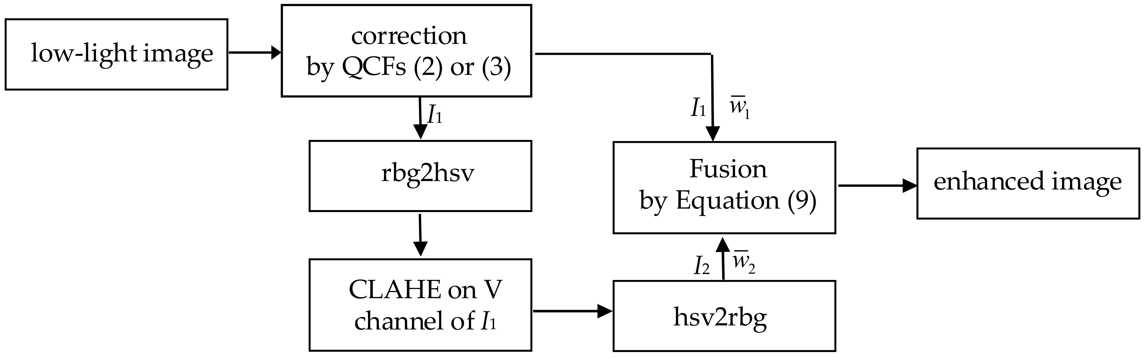
In this paper, we also propose a fusion-based method for enhancing low-light images, which is based on proposed quasi-symmetric correction functions (QCFs). Firstly, we present two couples of QCFs to obtain a globally- enhanced image for the original low-light image. Then, we employ CLAHE [17] on the value channel of the enhanced image just derived to obtain a locally- enhanced image. Finally, we merge them by a proposed multi-scale fusion formula. Our main contributions are as follows:
(1)
We define two couples of QCFs that can simultaneously achieve an impartial correction within dim regions and dazzling regions for low-light images through the proposed weighting-adding formula.
(2)
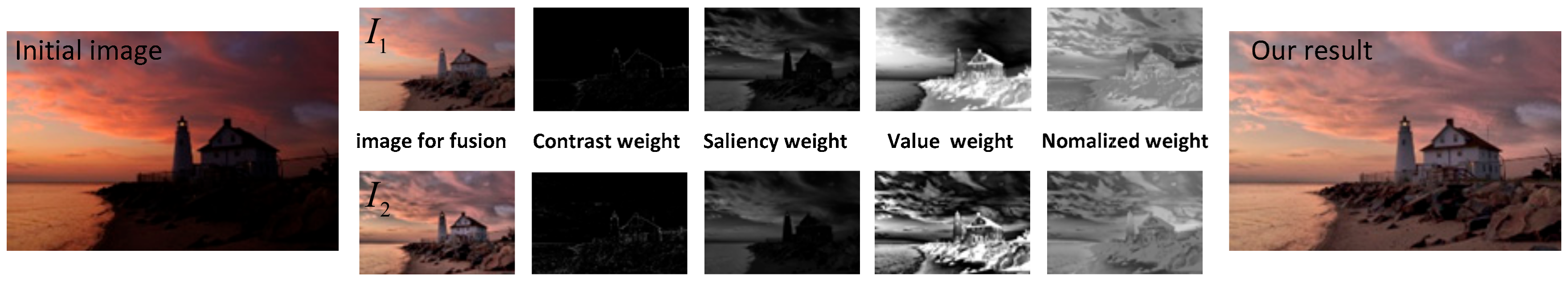
We define three weight maps which are effective for contrast improvement and detail preservation by fusion. In particular, we designed a value weight map, so we could achieve an excellent overall brightness for low-light images.
(3)
We achieved satisfactory enhancement results for low-light images based on defined QCFs by the proposed multi-scale fusion strategy, which aims to blend a globally-enhanced image and a locally-enhanced image.
The rest of the paper is organized as follows: In Section 2, two couples of QCFs are presented after introducing GC and the preliminary comparison experiment is shown. In Section 3, we propose a low-light image enhancement method based on QCFs by a delicately-designed fusion formula. In Section 4, comparison experimental results of different state-of-the-art methods are provided and their performance assessments are made and discussed. Finally, the conclusion is presented in Section 5.

2. Quasi-Symmetric Correction Functions (QCFs)

In the following, we will first give a brief introduction for traditional gamma correction and illustrate its shortcoming. Then we will define two couples of QCFs and show their successful results for image enhancement by a preliminary experiment based a simple weighting-adding formula.

2.1. Gamma Correction

GC maps the input low contrast image by [14]:
y = x γ , γ < 1
where x and y are the normalized input image and output image, respectively; and γ < 1 is a constant which is usually taken as 0.4545. GC has found many applications in image processing.
Figure 1 shows an original low-light image and its image enhanced by GC, from which it can be seen that the enhanced image has a better visual effect on the whole. However, its bright areas are also enlarged which makes them look so bright that the enhancement reduces local contrast within high-illuminance regions.

2.2. Quasi-Symmetric Correction Functions (QCFs)

To overcome the inherent defects of traditional GC, we designed two couples of quasi-symmetric correction functions (QCFs). The first couple comprise:
y 1 = x γ y 2 = 1 1 x 1 / γ γ
While the second couple comprise:
y 1 = 1 1 x 1 / γ y 2 = 1 1 x 1 / γ γ
Exponentiation computation is performed twice for the latter function of either couple of QCFs (2) or (3). Either couple of QCFs can be seen as two quasi-symmetric correction functions compared to the traditional gamma correction function (1).

2.3. Weighting-Adding Formula for QCFs

For either couple of QCFs, each pixel of the original image with weak light is processed by either function in the same way and hence the enhanced image is derived by:
y = α y 1 + 1 α y 2
where y i is the pixel value of transformed image by Equations (2) or (3) and α is a weighting factor which is determined by:
α = V ¯ h i g h V ¯ l o w V ¯ h i g h + V ¯ l o w
where V ¯ h i g h is mean of the top 10% value component (V) of the original low-light image in HSV color space and V ¯ l o w is the mean of the bottom 10%. On the one hand, any low-light image has very low contrast in both dark and bright regions, hence here we only take the key minority into consideration. On the other hand, the distribution for these pixels is relatively concentrated, so their means change little, as has been justified by the number of experiments on various low-light images.
Figure 2 shows the enhanced images by different correction methods including traditional GC, AGCWD [29], and our QCFs (2) and (3), respectively. We can easily find that all correction methods can improve the overall brightness. However, the GC and AGCWD approaches cause over-enhancement in bright areas. Overall, the method based on proposed QCFs can better preserve image details. In other words, by weighting-adding QCFs (2) or (3), we can achieve an impartial correction result for low-light images. The preliminary comparison experiment has shown the effectiveness of QCFs for low-light image enhancement. In order to further dig out their potential, we will improve the simple fusion based on the weighting-add method in the following section.

3. Low-Light Image Enhancement Based on QCFs by Fusion

In this section, we will propose a novel multi-scale fusion method to blend a globally-enhanced image and a locally-enhanced image obtained from original low-light image. In the following, we will describe the three main steps for multi-scale fusion.

3.1. Input Images Derived for Fusion

As described in Section 2, QCFs can improve the global contrast without losing detail information. Therefore, we can obtain the first input image ( I 1 ) for fusion by mapping the original low-light image according to Equations (4) and (5) based on QCFs (2) or (3). In order to further improve the local contrast and details, we can obtain the second input image ( I 2 ) for fusion by transforming I 1 from RGB space into HSV space, then exerting CLAHE on its value component and finally returning back to RGB space. Because the first input image ( I 1 ) used for fusion has gained high global visibility and the second input image ( I 2 ) has achieved clear local details, the multi-scale fusion-based method will greatly upgrade image quality and hence hopefully have a satisfactory result.

3.2. Weight Map Design

The weights for fusion greatly affect the quality of the fused image [4]. In this step, we develop a strategy for weight maps as in our previous work [35]. In order to make the fused image look better, the weight maps are pixel-level. We first normalized two input images. Then their global contrast, local salient feature, and value feature are taken into consideration to design the weight maps for fusion.
In the following, for either input image, I i , for fusion, we denote its contrast weight map, saliency weight map, and value weight map as w i , 1 , w i , 2 , and w i , 3 , respectively.

3.2.1. Contrast Weight Map Design

The contrast weight map ( w i , 1 ) is designed to estimate the global contrast. In [20], the contrast weight map is calculated by employing Laplacian sharpening, filtering to the L channel of the input image for fusion in Lab color space. In our case, we conducted Laplacian sharpening filtering to the value component in HSV space because it can assign edges and textures higher weights. As a result, it can hopefully make the edges of the fused image more prominent.

3.2.2. Saliency Weight Map Design

The saliency weight map ( w i , 2 ) is designed to highlight the object within low illumination regions and weaken image background. In [36], the saliency map is obtained by Euclidean distance between the Lab pixel vector in a Gaussian filtered image and the average Lab vector for the input image. However, this method tends to highlight the regions with high luminance values, so it is not suitable for low illumination colorful images. For any image with weak illumination, regions with low pixel values may contain the target object. For this reason, we redefine the saliency weight map as follows:
w i , 2 ( x , y ) = c I i c ( x , y ) m e a n { I i c } 2
the superscript c { R , G , B } denotes the RGB channel; and m e a n { } denotes mean operator.

3.2.3. Value Weight Map Design

The value weight map ( w i , 3 ) is designed to enable our fusion approach to adapt to the dim illumination environment of any captured low-light image. Considering the fact that images for fusion have different mean values, we normalize by them and obtain the following value weight map:
w i , 3 ( x , y ) = c I i c ( x , y ) m e a n { V i } 2 3 × m e a n { V i } 2
where V i represents the value component of the input image, I i , for fusion in HSV space. By incorporating the value weight map into the fusion process, the final enhanced image will certainly have an excellent overall brightness.

3.2.4. Final Normalized Weight Map

The normalized weight map ( w ¯ i ) is finally obtained by normalizing the above three weights by:
w ¯ i ( x , y ) = k w i , k ( x , y ) i k w i , k ( x , y )

3.3. Multi-Scale Fusion

So far, the desired fused image could be obtained by naive blending two input images with the normalized weight maps. However, the naive fusing approach often introduces undesirable artifacts and halos [37]. To overcome these shortcomings, many researchers apply traditional multi-scale fusion technology to avoid halos [5,38]. Methods based on multi-scale fusion can obtain a high-quality fused image by effectively extracting the features of input images. These methods employ Laplace operator to decompose each input image into Laplace pyramids [33] to extract image features, and employ Gaussian operator to decompose each normalized weight map into Gaussian pyramids to smooth the strong transitions. The levels of the Gaussian pyramids and Laplacian pyramids are same. The final enhanced result is then obtained by mixing them as follows:
I o u t p u t x , y = l U d i = 1 2 G l { w ¯ i ( x , y ) } L l { I i ( x , y ) }
where l represents the number of layers of the pyramids, U d is the up-sampling operator with d = 2 l 1 , and G { } and L { } represent Gaussian operator and Laplace operator, respectively.

3.4. Method Summary

We summarize the whole procedure of the proposed method in Figure 3. Figure 4 illustrates the results after each intermediate step. Here the first image ( I 1 ) for fusion in Figure 4 is obtained according to QCFs (2).

4. Results and Discussion

In this section, we present our experimental results and evaluate the performance of our method. First, we present our experiment settings. Then, we evaluate the proposed method by comparing it with other seven state-of-the-art methods in both subjective and objective aspects.

4.1. Experiment Settings

To fully evaluated the proposed method, we tested hundreds of images under different low illumination conditions from various scenes. All test images came from Wang et al. [17] and Loh et al. [39]. We performed all the experimental images in MATLAB R2017b on a PC running Windows 10 OS with 2.1 GHz Intel Pentium Dual Core Processor and 32G RAM.
In the following, we set l = 4 in (9), which denotes a moderate number of layers; and we set γ = 0.4545 in (2) and (3), which is just the traditional option. At the end of this section, we will analyze the sensitivity of the parameters l in (9), and γ in (2) and (3).

4.2. Subjective Evaluation

We compared the proposed method with seven methods proposed in recent years—naturalness-preserved enhancement algorithm (NPEA) [24], Fast-hue and range-preserving histogram specification (FPHS) [30], multi-scale fusion (MF) [33], bio-inspired multi-exposure fusion (BIMEF) [34], naturalness-preserved image enhancement using a priori multi-layer lightness statistics (NPIE) [26], low-light image enhancement via illumination map estimation (LIME) [31], and low-light image enhancement using the camera response model (LECARM) [32].
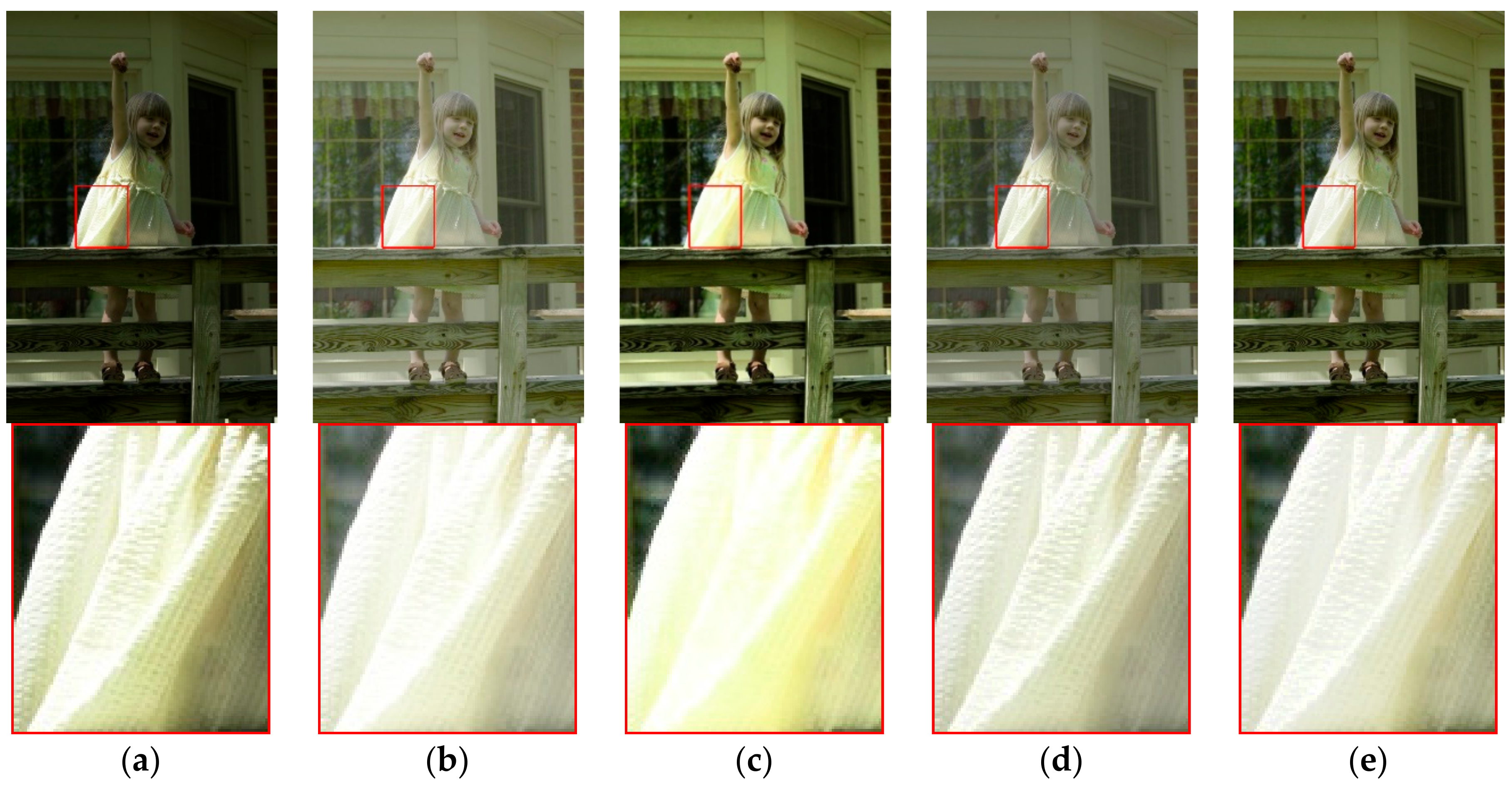
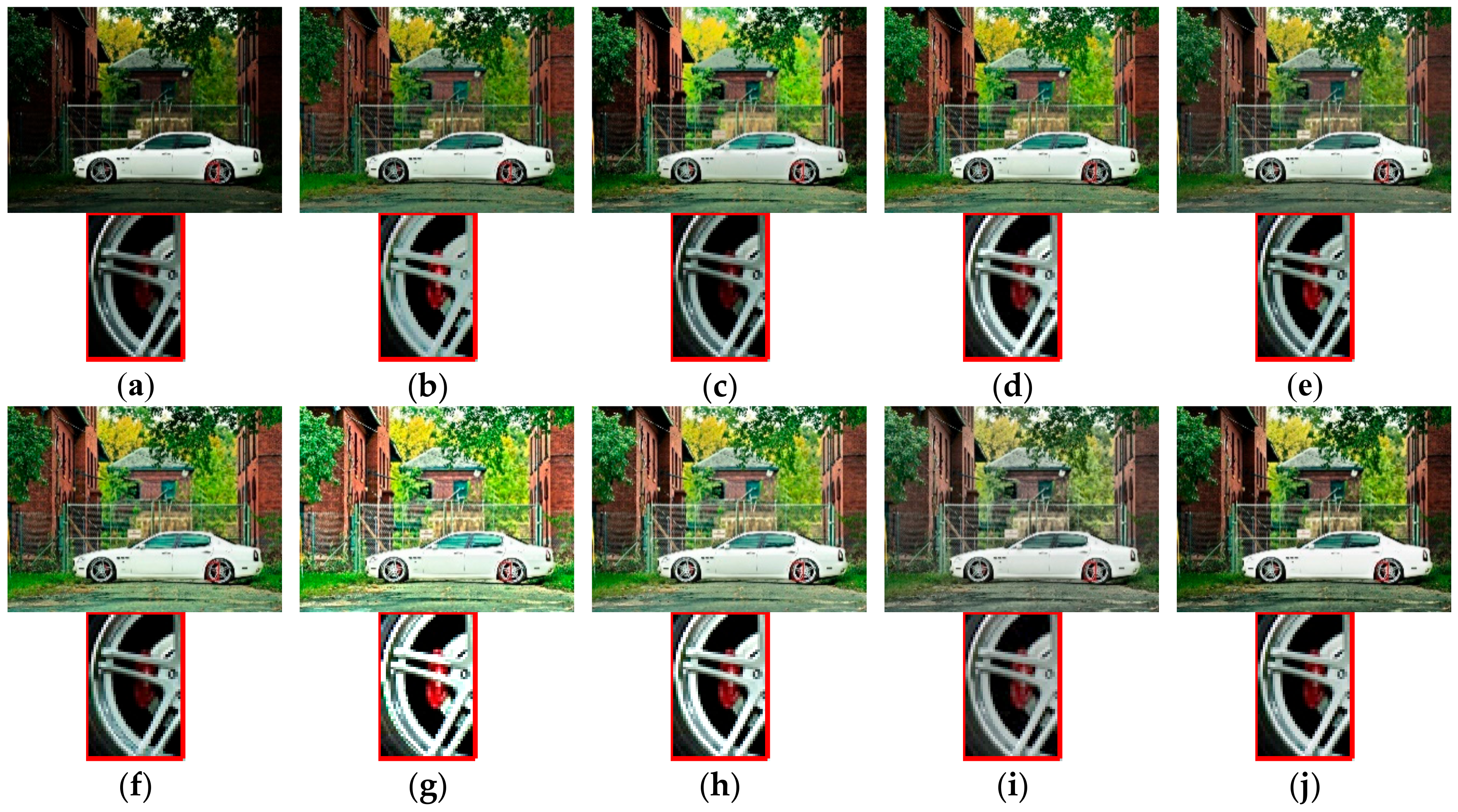
Five representative low-light images (“Car” shown in Figure 5, “Tree” shown in Figure 6, “Grass” shown in Figure 7, “Flower” shown in Figure 8, and “Tower” shown in Figure 9) and their enhanced results by different methods are shown in Figure 5, Figure 6, Figure 7, Figure 8 and Figure 9. Just below each original image or enhanced image are zoomed details which correspond to the small rectangular part within the bigger image.
NPEA is effective in preserving the naturalness of images, the colors of its results are vivid. However, it does not work well in very dark regions (the treetop in the third images), which results in artifacts and noise in the enhanced image. FPHS has the advantage of enlarging the difference between large regions, but it sometimes led to noise and halos (the light in the second image and the treetop in the third image) due to the merging of similar gray levels. As for MF, BIMEF, and LECARM, they all have good subjective evaluation. NPIE is similar to NPEA. Its results have a better visual effect than NPEA, but it also has the problem of artifacts (the treetop in the third images) and the runtime is too long. LIME effectively improves the overall brightness of the image especially in dark areas and enhances the details. Nevertheless, some regions such as the car in the first image suffer from over-enhancement. By contrast, the proposed method can produce satisfying results in most cases. Although the images enhanced by our method using QCFs (3) are a little dark, the details are effectively enhanced. Comparatively, our methods cannot only generate more natural results with no halo artifacts, but also successfully enhance the visibility of images with low illumination.

4.3. Objective Evaluation

Subjective evaluation alone is not convincing; therefore, we also need to evaluate the performance of our method objectively. There are a large number of objective image quality assessment (IQA) methods, including full-reference IQA [40], reduced-reference IQA [41], and no-reference IQA (NR-IQA) [42,43]. It is not easy to obtain ground truth images under ubiquitous non-uniform illumination conditions but here we adopt six no-reference IQA (NR-IQA) indexes for objective evaluation: natural image quality evaluator (NIQE) [42], integrated local NIQE (IL-NIQE) [43], lightness-order error (LOE) [24], no-reference image quality metric for contrast distortion (NIQMC) [44], colorfulness-based patch-based contrast quality index (C-PCQI) [45], and oriented gradients image quality assessment (OG-IQA) [46].
NIQE builds a simple and successful space domain natural scene statistic model and then extracts features from it to construct a “quality aware” collection of statistical features. It can measure deviations from statistical regularities. IL-NIQE can successfully obtain local distortion artifacts by integrating the features of natural image statistics derived from a local multivariate Gaussian model. LOE measures the error between the original image and its enhanced version to objectively evaluate the naturalness preservation. Lower values for NIQE, IL-NIQE, and LOE, all indicate better image quality. NIQMC is based on the concept of information maximization and can accurately judge which has larger contrast and better quality between two images. C-PCQI yields a measure of visual quality using a regression module of 17 features through analysis of contrast, sharpness, and brightness. OG-IQA can effective provide quality-aware sources of information by using the image relative gradient orientation. Higher values for NIQMC, C-PCQI, and OG-IQA, all indicate better image quality.
Six IQA indexes for the five low-light images shown in Figure 5, Figure 6, Figure 7, Figure 8 and Figure 9 by different methods are given in Table 1, Table 2, Table 3, Table 4, Table 5 and Table 6, respectively. The bolding of the numbers denotes the best one.
Moreover, to verify the stability of the proposed method, the average assessment results of 100 images are given in Table 7. One can see that the scores for NIQE and IL-NIQE, that were acquired from our method based on QCFs (2), both rank first, and the scores for NIQMC, OG-IQA, and LOE rank second, third, and fourth out of nine, respectively. One can see that the score for C-PCQI, which is acquired from our method based on QCFs (3), ranks first, the scores for both IL-NIQE and LOE rank second out of nine, and the scores for OG-IQA and NIQMC are in equal third place and equal fourth place, respectively. Hence, we can come to a conclusion that our method based on QCFs (2) achieves the best high-quality for image enhancement and has medium capability of naturalness preservation. Objectively speaking, our method based on QCFs (3) also achieves good scores and hence has good potential for image enhancement.
Furthermore, we present the analysis of variance (ANOVA) of the nine involved methods for the 100 test images on six IQA indexes to show the different characteristics of each method. The ANOVA table is listed in Table 8. The results show that these methods have no significant difference for both NIQE and OG-IQA.
The post hoc multiple comparison test was also conducted using the Matlab function “multcompare”. The significant difference results from QCFs (2) and (3) for different indexes are shown in Figure 10 and Figure 11, respectively. The numbers of significant different groups from QCFs (2) and (3) for different indexes are listed in Table 9.
The timing performance of different methods is given in Table 10. In general, any algorithm, which is based on iterative learning or machine learning, such as NPEA, FHHS, NPIE, or LIME, is time-consuming. Compared to other methods, our method has a moderate computational performance, since it does not need iteration to output results.

4.4. Sensitivity of the Parameters l and γ

The sensitivity of parameter l in (9) and parameter γ in (2) and (3) are also compared.
With respect to the number of layers of the pyramids in the fusion procedure (9), we set l = 4 from the perspective of comprehensive consideration of performance and payload. From the above experiments, we can see that the choice was appropriate. Now we first fix γ in QCFs (2) or (3), then enumerate a small range of values around 4 and compute the corresponding average performance indexes for QCFs (2) and (3). The results for QCFs (2) and (3) with different l and γ = 0.4545 are reported in Table 11 and Table 12, respectively. There is only a slight difference between the indexes from different l. 
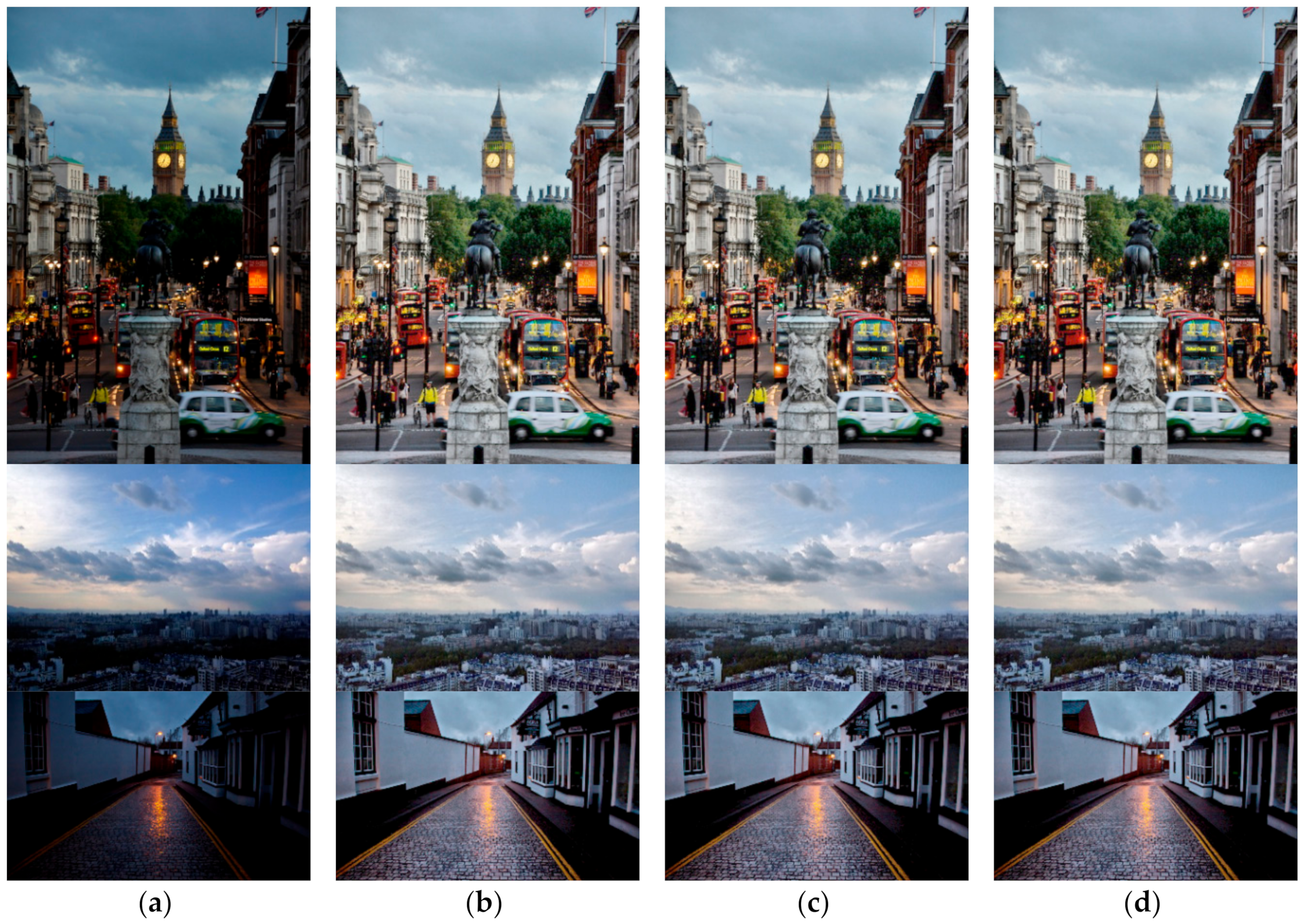
Figure 12 shows three low-light images and the corresponding enhanced ones with l = 3, 4, and 5, respectively. From Figure 12 we can see that the enhanced images from different l do not differ much in visual effect. We can see the enhanced images from l = 4 have high contrast and satisfactory details. Comprehensively considering indicators and visual effects, one can conclude that l = 4 is a good selection.
As far as the parameter γ is concerned, the experiments were analogous. We set its value around 0.4545, and the corresponding average performance indexes with fixed l for QCFs (2) and (3) were calculated. The results for QCFs (2) and (3) with different γ and l = 4 are reported in Table 13 and Table 14, respectively. One can see that the parameter γ = 0.4545 can balance payload and performance and hence is a good selection.

5. Conclusions

In this paper, we first define two couples of quasi-symmetric correction functions (QCFs) to enhance low-light images. Compared with traditional gamma correction, proposed QCFs cannot only improve the overall image brightness, but also can better preserve image details. Moreover, we propose an effective multi-scale fusion method to combine a globally-enhanced image by QCFs and a local enhanced image by CLAHE. Experiment results from many images showed that our method can significantly improve the contrast of low-light images and successfully achieve a balanced detail enhancement for dark regions and bright regions. From the perspective of subjective evaluation and objective evaluation, our proposed method has a better performance than other state-of-the-art methods. As future work, we will try to apply the proposed QCFs for image dehazing, underwater image enhancement, and image enhancement in poor visibility conditions and so on. We will also explore applications of QCFs in automatic and on-line detection system for product defects and real-time intelligent monitoring for production lines based on machine vision.

Author Contributions

Funding acquisition, C.L.; methodology, C.L., S.T., J.Y., and T.Z.; supervision, C.L.; validation, S.T. and T.Z.; writing—original draft, S.T.; writing—review and editing, C.L. and T.Z., C.L., and S.T. contributed equally to this work. All authors have read and agreed to the published version of the manuscript.

Funding

This research was funded by the open fund of Guangdong Provincial Key Laboratory of Digital Signal and Image Processing Technology, the National Natural Science Foundation of China under grant Nos. 61871174 and 61902232, and the 2020 Li Ka Shing Foundation Cross-Disciplinary Research Grant (No. 2020LKSFG05D).

Acknowledgments

We would like to thank the anonymous reviewers for their kind comments and valuable suggestions which have greatly improved our manuscript.

Conflicts of Interest

The authors declare no conflict of interest.

Abbreviations

GCGamma correction
QCFsQuasi-symmetric correction functions
HEHistogram equalization
AHEAdaptive histogram equalization
CLAHEContrast limited adaptive histogram equalization
LDRLayered difference representation
NPEANaturalness-preserved enhancement algorithm
AGCWDAdaptive gamma correction with weighting distribution
FPHSFast hue and range-preserving histogram specification
MFMulti-scale fusion
BIMEFBio-inspired multi-exposure fusion
NPIENaturalness-preserved image enhancement using a priori multi-layer lightness statistics
LIMELow-light image enhancement via illumination map estimation
LECARMLow-light image enhancement using the CAmera response model
IQAImage quality assessment
NR-IQANo-reference IQA
NIQENatural image quality evaluator
IL-NIQEIntegrated local NIQE
LOELightness order error
NIQMCNo-reference image quality metric for contrast distortion
C-PCQIColorfulness-based patch-based contrast quality index
OG-IQAOriented gradients image quality assessment

References

  1. Redmon, J.; Divvala, S.; Girshick, R.; Farhadi, A. You only look once: Unified, real-time object detection. In Proceedings of the 2016 IEEE Conference on Computer Vision and Pattern Recognition (CVPR), Las Vegas, NV, USA, 27–30 June 2016; pp. 779–788. [Google Scholar]
  2. Wang, J.; Wang, W.; Wang, R.; Gao, W. CSPS: An adaptive pooling method for image classification. IEEE Trans. Multimed. 2016, 18, 1000–1010. [Google Scholar] [CrossRef]
  3. Ancuti, C.; Ancuti, C.O.; Haber, T.; Bekaert, P. Enhancing underwater images and videos by fusion. In Proceedings of the 2012 IEEE Conference on Computer Vision and Pattern Recognition (CVPR), Providence, RI, USA, 16–21 June 2012; pp. 81–88. [Google Scholar]
  4. Ancuti, C.O.; Ancuti, C. Single image dehazing by multi-scale fusion. IEEE Trans. Image Process. 2013, 22, 3271–3282. [Google Scholar] [CrossRef] [PubMed]
  5. Fu, X.; Zeng, D.; Huang, Y.; Liao, Y.; Ding, X.; Paisley, J. A fusion-based enhancing method for weakly illuminated images. Signal Process. 2016, 129, 82–96. [Google Scholar] [CrossRef]
  6. Wang, J.; Shih, M.; Wang, C. Novel framework for optical film defect detection and classification. IEEE Access 2020, 8, 60964–60978. [Google Scholar]
  7. Lia, C.; Zhang, X.; Huang, Y.; Tang, C.; Fatikow, S. A novel algorithm for defect extraction and classification of mobile phone screen based on machine vision. Comput. Ind. Engin. 2020, 146, 106530. [Google Scholar] [CrossRef]
  8. Deng, Y.; Xu, S.; Lai, W. A novel imaging-enhancement-based inspection method for transparent aesthetic defects in a polymeric polarizer. Polym. Test. 2017, 61, 133–140. [Google Scholar] [CrossRef]
  9. Peli, E. Contrast in complex images. J. Opt. Soc. Amer. A Opt. Image Sci. 1990, 7, 2032–2040. [Google Scholar] [CrossRef]
  10. Beghdadi, A.; Negrate, A.L. Contrast enhancement technique based on local detection of edges. Comput. Vis. Graph. Image Process. 1989, 46, 162–174. [Google Scholar] [CrossRef]
  11. Gonzalez, R.; Woods, R. Digital Image Processing; Prentice-Hall: Upper Saddle River, NJ, USA, 2008. [Google Scholar]
  12. Bovik, A.C. Handbook of Image and Video Processing; Academic: New York, NY, USA, 2010. [Google Scholar]
  13. Lee, C.; Kim, C.S. Contrast enhancement based on layered difference representation of 2D histograms. IEEE Trans. Image Process. 2013, 22, 5372–5384. [Google Scholar] [CrossRef]
  14. Poynton, C.A. Gamma and its disguises: The nonlinear mappings of intensity in perception, CRTs, film, and video. SMPTE J. 1993, 102, 1099–1108. [Google Scholar] [CrossRef]
  15. Pizer, S.M.; Amburn, P.; Austin, J.D.; Cromartie, R.; Geselowitz, A.; Greer, T.; ter Haar Romeny, B.; Zimmerman, J.B.; Zuiderveld, K. Adaptive histogram equalization and its variations. Comput. Vis. Graph. Image Process. 1987, 39, 355–368. [Google Scholar] [CrossRef]
  16. Li, X.; Bai, L.; Ge, Z.; Yang, X.; Zhou, T. Early diagnosis of neuropsychiatric systemic lupus erythematosus by deep learning enhanced magnetic resonance spectroscopy. J. Med. Imaging Health Inform. 2021, 1. in press. [Google Scholar]
  17. Reza, A.M. Realization of the contrast limited adaptive histogram equalization (CLAHE) for real-time image enhancement. J. VLSI Signal Process. Syst. Signal Image Video Technol. 2004, 38, 35–44. [Google Scholar] [CrossRef]
  18. Zuiderveld, K. Contrast limited adaptive histogram equalization. In Graphics Gems IV; Academic Press Professional: San Diego, CA, USA, 1994; pp. 474–485. [Google Scholar]
  19. Abdullah-Al-Wadud, M.; Kabir, M.H.; Dewan, M.A.A.; Chae, O. A dynamic histogram equalization for image contrast enhancement. IEEE Trans. Consum. Electron. 2007, 53, 593–600. [Google Scholar] [CrossRef]
  20. Land, E.H. The retinex theory of color vision. Sci. Am. 1977, 237, 108–128. [Google Scholar] [CrossRef]
  21. Jobson, D.J.; Rahman, Z.-U.; Woodell, G.A. A multiscale Retinex for bridging the gap between color images and the human observation of scenes. IEEE Trans. Image Process. 1997, 6, 965–976. [Google Scholar] [CrossRef] [Green Version]
  22. Elad, M.; Kimmel, R.; Shaked, D.; Keshet, R. Reduced complexity retinex algorithm via the variational approach. J. Vis. Commun. Image Represent. 2003, 14, 369–388. [Google Scholar] [CrossRef]
  23. Hines, G.; Rahman, Z.-U.; Jobson, D.; Woodell, G. Single-scale Retinex using digital signal processors. Glob. Signal Process. Expo 2004, 2, 335–343. [Google Scholar]
  24. Wang, S.; Zheng, J.; Hu, H.; Li, B. Naturalness preserved enhancement algorithm for non-uniform illumination images. IEEE Trans. Image Process. 2013, 22, 3538–3548. [Google Scholar] [CrossRef]
  25. Fu, X.; Liao, Y.; Zeng, D.; Huang, Y.; Zhang, X.P.; Ding, X. A probabilistic method for image enhancement with simultaneous illumination and reflectance estimation. IEEE Trans. Image Process. 2015, 24, 4965–4977. [Google Scholar] [CrossRef]
  26. Wang, S.; Luo, G. Naturalness preserved image enhancement using a priori multi-layer lightness statistics. IEEE Trans. Image Process. 2018, 27, 938–948. [Google Scholar] [CrossRef] [PubMed]
  27. Cai, B.; Xu, X.; Guo, K.; Hu, B.; Tao, D. A joint intrinsic extrinsic prior model for Retinex. In Proceedings of the 2017 IEEE International Conference on Computer Vision Workshops, Venice, Italy, 22–29 October 2017; pp. 4000–4009. [Google Scholar]
  28. Xu, J.; Hou, Y.; Ren, D.; Liu, L.; Zhu, F.; Yu, M.; Wang, H.; Shao, L. STAR: A structure and texture aware Retinex model. IEEE Trans. Image Process. 2020, 29, 5022–5037. [Google Scholar] [CrossRef] [PubMed] [Green Version]
  29. Huang, S.; Cheng, F.; Chiu, Y. Efficient contrast enhancement using adaptive gamma correction with weighting distribution. IEEE Trans. Image Process. 2013, 22, 1032–1041. [Google Scholar] [CrossRef] [PubMed]
  30. Nikolova, M.; Steidl, G. Fast hue and range preserving histogram specification: Theory and new algorithms for color image enhancement. IEEE Trans. Image Process. 2014, 23, 4087–4100. [Google Scholar] [CrossRef] [PubMed] [Green Version]
  31. Guo, X.; Li, Y.; Ling, H. LIME: Low-light image enhancement via illumination map estimation. IEEE Trans. Image Process. 2017, 26, 982–993. [Google Scholar] [CrossRef]
  32. Ren, Y.; Ying, Z.; Li, T.; Li, G. LECARM: Low-light image enhancement using the camera response model. IEEE Trans. Circuits Syst. Video Technol. 2019, 29, 968–981. [Google Scholar] [CrossRef]
  33. Burt, P.; Adelson, T. The Laplacian pyramid as a compact image code. IEEE Trans. Commun. 1983, 31, 532–540. [Google Scholar] [CrossRef]
  34. Ying, Z.; Li, G.; Gao, W. A Bio-Inspired Multi-Exposure Fusion Framework for Low-Light Image Enhancement. arXiv 2017, arXiv:1711.00591. [Google Scholar]
  35. Tang, S.; Li, C. Low illumination image enhancement based on image fusion. In Proceedings of the 3rd International Conference on Pattern Recognition and Artificial Intelligence (PRAI), Chengdu, China, 28–30 August 2020. [Google Scholar]
  36. Achantay, R.; Hemamiz, S.; Estraday, F.; Susstrunk, S. Frequency-tuned salient region detection. In Proceedings of the IEEE CVPR, Miami, FL, USA, 20–25 June 2009; pp. 1597–1604. [Google Scholar]
  37. Wang, Q.; Fu, X.; Zhang, X.; Ding, X. A fusion-based method for single backlit image enhancement. In Proceedings of the IEEE International Conference on Image Processing (ICIP), Phoenix, AZ, USA, 25–28 September 2016; pp. 4077–4081. [Google Scholar]
  38. Mertens, T.; Kautz, J.; Van Reeth, F. Exposure fusion: A simple and practical alternative to high dynamic range photography. Comput. Graph. Forum 2009, 28, 161–171. [Google Scholar] [CrossRef]
  39. Loh, Y.P.; Chan, C.S. Getting to know low-light images with the exclusively dark dataset. Comput. Vis. Image Underst. 2019, 178, 30–42. [Google Scholar] [CrossRef] [Green Version]
  40. Wang, Z.; Bovik, A.C.; Sheikh, H.R.; Simoncelli, E.P. Image quality assessment: From error visibility to structural similarity. IEEE Trans. Image Process. 2004, 13, 600–612. [Google Scholar] [CrossRef] [Green Version]
  41. Min, X.; Gu, K.; Zhai, G.; Hu, M.; Yang, X. Saliency-induced reduced-reference quality index for natural scene and screen content images. Signal Process. 2018, 145, 127–136. [Google Scholar] [CrossRef]
  42. Mittal, A.; Soundarajan, R.; Bovik, A.C. Making a “completely blind” image quality analyzer. IEEE Signal Process. Lett. 2012, 20, 209–212. [Google Scholar] [CrossRef]
  43. Zhang, L.; Zhang, L.; Bovik, A.C. A feature-enriched completely blind image quality evaluator. IEEE Trans. Image Process. 2015, 24, 2579–2591. [Google Scholar] [CrossRef] [PubMed] [Green Version]
  44. Gu, K.; Lin, W.; Zhai, G.; Yang, X.; Zhang, W.; Chen, C.W. No-reference quality metric of contrast-distorted images based on information maximization. IEEE Trans. Cybern. 2017, 47, 4559–4565. [Google Scholar] [CrossRef] [PubMed]
  45. Gu, K.; Tao, D.; Qiao, J. Lin, W. Learning a no-reference quality assessment model of enhanced images with big data. IEEE Trans. Neural Netw. Learn. Syst. 2018, 29, 1301–1313. [Google Scholar] [CrossRef] [PubMed] [Green Version]
  46. Liu, L.; Hua, Y.; Zhao, Q.; Huang, H.; Bovik, A.C. Blind image quality assessment by relative gradient statistics and Adaboosting neural network. Signal Process. Image Commun. 2016, 40, 1–15. [Google Scholar] [CrossRef]
Figure 1. Low-light image enhancement by gamma correction (GC). (a) Original low-light image and (b) image enhanced by GC.
Symmetry 12 01561 g001
Figure 2. Low-light image enhanced by different correction methods. (a) Input image, (b) enhanced by GC, (c) enhanced by adaptive gamma correction with weighting distribution (AGCWD) [29], and (d) enhanced by QCFs (2), and (e) QCFs (3).
Symmetry 12 01561 g002
Figure 3. Flowchart of proposed low-light image enhancement method.
Symmetry 12 01561 g003
Figure 4. Results after each intermediate step of our method. From left to the right, original low-light image, two input images for fusion, the three weight maps, the normalized weight maps, and our enhanced result.
Symmetry 12 01561 g004
Figure 5. Images of “Car” enhanced by different methods. (a) Original “Car” image; images enhanced by (b) naturalness-preserved enhancement algorithm (NPEA) [24], (c) Fast-hue and range-preserving histogram specification (FHHS) [30], (d) multi-scale fusion (MF) [5], (e) bio-inspired multi-exposure fusion (BIMEF) [34], (f) naturalness-preserved image enhancement (NPIE) [26], (g) low-light image enhancement via illumination map estimation (LIME) [31], (h) low-light image enhancement using the camera response model (LECARM) [32], and by proposed methods based on (i) QCFs (2) and (j) QCFs (3), respectively.
Symmetry 12 01561 g005
Figure 6. Images of “Tree” enhanced by different methods. (a) Original “Tree” image; images enhanced by (b) NPEA [24], (c) FHHS [30], (d) MF [5], (e) BIMEF [34], (f) NPIE [26], (g) LIME [31], (h) LECARM [32], and by proposed methods based on (i) QCFs (2) and (j) QCFs (3), respectively.
Symmetry 12 01561 g006
Figure 7. Images of “Grass” enhanced by different methods. (a) Original “Grass” image; images enhanced images by (b) NPEA [24], (c) FHHS [30], (d) MF [5], (e) BIMEF [34], (f) NPIE [26], (g) LIME [31], (h) LECARM [32], and by proposed methods based on (i) QCFs (2) and (j) QCFs (3), respectively.
Symmetry 12 01561 g007
Figure 8. Enhanced images for “Flower” by different methods. (a) Original “Flower” image; images enhanced images by (b) NPEA [24], (c) FHHS [30], (d) MF [5], (e) BIMEF [34], (f) NPIE [26], (g) LIME [31], (h) LECARM [32], and by proposed methods based on (i) QCFs (2) and (j) QCFs (3), respectively.
Symmetry 12 01561 g008
Figure 9. Enhanced images for “Tower” by different methods. (a) original “Tower” image; enhanced images by (b) NPEA [24], (c) FHHS [30], (d) MF [5], (e) BIMEF [34], (f) NPIE [26], (g) LIME [31], (h) LECARM [32], and by proposed methods based on (i) QCFs (2) and (j) QCFs (3), respectively.
Symmetry 12 01561 g009
Figure 10. Significant difference from QCFs (3) for different indexes. From top to bottom, the horizontal axis denotes nine methods, viz., 1 for NPEA [15], 2 for FHHS [26], 3 for MF [25], 4 for BIMEF [28], 5 for NPIE [17], 6 for LIME, 7 for LECARM [30], 8 for QCFs (2), and 9 for QCFs (3), respectively. (a) NIQE, (b) IL-NIQE, (c) LOE, (d) NIQMC, (e) C-PCQI, and (f) OG-IQA.
Symmetry 12 01561 g010
Figure 11. Significant difference from QCFs (2) for different indexes. From top to bottom, the horizontal axis denotes nine methods, viz., 1 for NPEA [15], 2 for FHHS [26], 3 for MF [25], 4 for BIMEF [28], 5 for NPIE [17], 6 for LIME, 7 for LECARM [30], 8 for QCFs (2), and 9 for QCFs (3), respectively. (a) NIQE, (b) IL-NIQE, (c) LOE, (d) NIQMC, (e) C-PCQI, and (f) OG-IQA.
Symmetry 12 01561 g011
Figure 12. Enhanced images by different numbers of layers of pyramids in (9). (a) Original low-light images; images enhanced with (b) l = 3 in (9), (c) l = 4 in (9), and (d) l = 5 in (9), respectively.
Symmetry 12 01561 g012
Table 1. Assessment results of natural image quality evaluator (NIQE) (↓) for different methods.
ImagesNPEAFHHSMFBIMEFNPIELIMELECARMQCFs (2)QCFs (3)
Car1.782.872.021.541.882.331.761.681.75
Tree2.142.432.312.162.172.642.251.972.09
Grass2.442.382.282.002.383.082.301.982.27
Flower2.732.952.762.552.732.752.472.592.51
Tower3.343.303.723.233.133.673.573.073.30
Mean2.492.792.622.302.462.892.472.252.38
Table 2. Assessment results of integrated local NIQE (IL-NIQE) (↓) for different methods.
ImagesNPEAFHHSMFBIMEFNPIELIMELECARMQCFs (2)QCFs (3)
Car20.9318.6519.8819.1321.7025.1020.3817.0819.48
Tree18.7619.0820.0119.1017.7518.7619.1118.8518.20
Grass21.0318.8020.2218.7620.2225.4419.7218.5019.15
Flower20.5018.0118.0218.0519.9928.8418.0617.5318.15
Tower19.0216.7520.5720.5919.4419.4219.1516.9818.05
Mean20.0518.2619.7419.1319.8223.4919.2817.7918.61
Table 3. Assessment results of lightness-order error (LOE) (↓) for different methods.
ImagesNPEAFHHSMFBIMEFNPIELIMELECARMQCFs (2)QCFs (3)
Car785852866813847842857866846
Tree668861839656855779863804627
Grass362717618520788863718599449
Flower692826842702859878860823770
Tower9029781035958834101410591029954
Mean681841840729836875871824729
Table 4. Assessment results of no-reference image quality metric for contrast distortion (NIQMC) () for different methods.
ImagesNPEAFHHSMFBIMEFNPIELIMELECARMQCFs (2)QCFs (3)
Car5.425.745.705.515.755.805.805.765.72
Tree5.135.475.715.415.455.205.655.455.50
Grass5.325.335.445.395.405.515.545.505.52
Flower5.375.725.745.365.595.475.765.515.60
Tower4.945.655.124.835.135.135.115.185.24
Mean5.245.585.545.305.465.425.575.485.51
Table 5. Assessment results of colorfulness-based patch-based contrast quality index (C-PCQI) () for different methods.
ImagesNPEAFHHSMFBIMEFNPIELIMELECARMQCFs (2)QCFs (3)
Car1.071.041.091.041.101.001.051.031.13
Tree1.060.981.121.031.081.011.061.051.12
Grass1.120.931.161.081.161.051.131.051.14
Flower1.020.961.061.041.070.961.050.991.09
Tower1.010.981.040.971.060.940.970.981.05
Mean1.060.981.091.031.090.991.051.021.11
Table 6. Assessment results of oriented gradients image quality assessment (OG-IQA) () for different methods.
ImagesNPEAFHHSMFBIMEFNPIELIMELECARMQCFs (2)QCFs (3)
Car0.760.710.710.720.760.740.710.720.70
Tree0.840.910.870.870.830.770.850.880.88
Grass0.860.890.840.870.840.800.850.860.89
Flower0.760.890.840.870.840.800.850.860.87
Tower0.710.740.650.710.670.650.650.670.74
Mean0.790.830.780.810.790.750.780.800.82
Table 7. Average performance of 100 images for different methods. The bolding of the numbers denotes the best one.
MetricNPEAFHHSMFBIMEFNPIELIMELECARMQCFs (2)QCFs (3)
NIQE (↓)3.043.243.083.032.993.123.032.983.07
IL-NIQE (↓)22.2922.2222.5321.5522.1724.6522.2820.7721.42
LOE (↓)695786788703795804818782701
NIQMC ()5.015.425.225.055.275.375.265.395.27
C-PCQI ()1.031.011.071.011.060.991.021.011.09
OG-IQA ()0.760.740.730.730.750.720.740.740.74
Table 8. One way of ANOVA of different IQA indexes.
ANOVASourceSSdfMSFProb > F
NIQEColumns5.07680.634440.620.7609
Error910.6538911.02206
Total915.728899
IL-NIQEColumns1157.98144.7344.691.20 × 10−5
Error2748289130.844
Total28639.8899
LOEColumns2.03e+-682538316.641.86 × 10−8
Error3.41e+0789138224.4
Total3.61e+07899
NIQMCColumns18.39582.2993716.072.62 × 10−22
Error127.4878910.14308
Total145.882899
C-PCQIColumns0.8691280.1086420.696.48 × 10−29
Error4.679058910.00525
Total5.54816899
OG-IQAColumns0.187780.023461.040.4028
Error20.07378910.02253
Total20.2614899
Table 9. The numbers of significant different groups from QCFs (2) and (3) for different indexes.
MethodNIQEIL-NIQELOENIQMCC-PCQIOG-IQA
QCFs (2)012340
QCFs (3)016360
Table 10. Average computational time (seconds) of 100 images for different methods.
NPEAFHHSMFBIMEFNPIELIMELECARMQCFs (2)QCFs (3)
26.211.70.80.542.118.50.65.96.8
Table 11. Sensitivity of l in (9) with γ = 0.4545 in QCFs (2).
lNIQEIL-NIQELOENIQMCC-PCQIOG-IQATime (s)
32.9820.817835.191.010.745.8
42.9820.777825.191.010.745.9
52.9820.757805.191.010.746.1
Table 12. Sensitivity of l in (9) with γ = 0.4545 in QCFs (3).
lNIQEIL-NIQELOENIQMCC-PCQIOG-IQATime (s)
33.0721.457035.261.080.746.5
43.0721.427015.271.090.746.8
53.0721.416995.271.090.747.0
Table 13. Sensitivity of γ in QCFs (2) with l = 4 in (9).
γ NIQEIL-NIQELOENIQMCC-PCQIOG-IQATime (s)
0.42.9820.747985.160.98−0.746.5
0.45452.9820.777825.191.01−0.745.9
0.52.9820.787655.211.03−0.745.5
Table 14. Sensitivity of γ in QCFs(3) with l = 4 in (9).
γ NIQEIL-NIQELOENIQMCC-PCQIOG-IQATime (s)
0.43.0821.406725.281.07−0.757.2
0.45453.0721.427015.271.09−0.746.8
0.53.0721.437235.261.10−0.746.9

