Fuzzy Goal Programming with an Imprecise Intuitionistic Fuzzy Preference Relations

Abstract

Fuzzy goal programming (FGP) is applied to solve fuzzy multi-objective optimization problems. In FGP, the weights are associated with fuzzy goals for the preference among them. However, the hierarchy within the fuzzy goals depends on several uncertain criteria, decided by experts, so the preference relations are not always easy to associate with weight. Therefore, the preference relations are provided by the decision-makers in terms of linguistic relationships, i.e., goal A is slightly or moderately or significantly more important than goal B. Due to the vagueness and ambiguity associated with the linguistic preference relations, intuitionistic fuzzy sets (IFSs) are most efficient and suitable to handle them. Thus, in this paper, a new fuzzy goal programming with intuitionistic fuzzy preference relations (FGP-IFPR) approach is proposed. In the proposed FGP-IFPR model, an achievement function has been developed via the convex combination of the sum of individual grades of fuzzy objectives and amount of the score function of IFPRs among the fuzzy goals. As an extension, we presented the linear and non-linear, namely, exponential and hyperbolic functions for the intuitionistic fuzzy preference relations (IFPRs). A study has been made to compare and analyze the three FGP-IFPR models with intuitionistic fuzzy linear, exponential, and hyperbolic membership and non-membership functions. For solving all three FGP-IFPR models, the solution approach is developed that established the corresponding crisp formulations, and the optimal solution are obtained. The validations of the proposed FGP-IFPR models have been presented with an experimental investigation of a numerical problem and a banking financial statement problem. A newly developed distance measure is applied to compare the efficiency of proposed models. The minimum value of the distance function represents a better and efficient model. Finally, it has been found that for the first illustrative problem considered, the exponential FGP-IFPR model performs best, whereas for the second problem, the hyperbolic FGP-IFPR model performs best and the linear FGP-IFPR model shows worst in both cases.

1. Introduction

Multi-objective programming is a robust analytical method for the formulation of real-world problems in which two or more than two goals have to be optimized, simultaneously. It has been favourably implemented for various applications in the field of engineering, economics, machine learning, manpower planning etc., see Ull Hasan et al. [1], Hasan and Hasan [2], Hasan et al. [3,4], Ashraf et al. [5,6], Muhuri et al. [7], Suttorp and Igel [8], Marler and Arora [9], Alexandropoulos et al. [10], Bora et al. [11], Breen et al. [12], Kumar et al. [13], Palacios [14], Nepomuceno [15], Caqo et al. [16], Ashraf et al. [17], Zheng et al. [18], Yang and Chou [19].

The mathematical formulation of classical multi-objective programming is as follows:

$$\begin{array}{cc}\hfill \mathrm{Max}\left(\mathrm{Min}\right):& \left\{Z_1\left(X\right),Z_2\left(X\right),\dots ,Z_K\left(X\right)\right\},\hfill \end{array}$$

(1)

$$\begin{array}{cc}\hfill \mathrm{subject}\mathrm{to}& Ax\le b\hfill \end{array}$$

(2)

$$\begin{array}{cc}\hfill & x\ge 0,x\in S.\hfill \end{array}$$

(3)

where $Z_k\left(X\right)\forall k=1,2,\dots ,K$ represents the k-th objective function of decision variable X and S is the set of feasible solutions. Equation (2) represents the constraints of the optimization problem where A and b are the $m\times n$ and $n\times 1$ dimensional matrices, respectively.

Goal programming (GP) is a regularly used methodology to overcome the multi-objective programming problems. Since, the initial proposal of GP by Charnes et al. Charnes et al. [20], Charnes and Cooper [21], several researchers, including Ignizio [22], Ignizio [23], Romero [24], Romero [25], Chang [26], Caballero and Go [27] and others expanded it theoretically as well practically. GP performs with the over-optimistic and under-pessimistic accomplishment of the objectives (goals) so that each goal is met with the smallest divergence from their particular target. In traditional GP, the aspiration level provides the best achievement value with the respective goal are explicitly acknowledged, though in real-world applications, the aspiration levels in the multi-objective decision-making problem are mostly not-precise. As a result, over the years, the principles of the fuzzy set approach was successfully utilized in GP.

Zadeh [28] initially offered the fuzzy sets (FSs). Following the proposal of FSs, Bellman and Zadeh [29] elaborated the decision approach in the imprecise context. Uncertainties, incorporated in GPs, due to the vagueness and ambiguity, are being handled by the concept of fuzzy decisions. The significance of accomplishment within every optimizing goal is greatly enhanced in fuzzy optimization methods, which enables the decision-maker (DM) to determine the best suitable result. The judgement of DM gets more and more difficult as the problem requires vague preferences for the target goals and their level of aspiration. Many researchers propose fuzzy goal programming (FGP) models, for example, Chen and Tsai [30], Aköz and Petrovic [31], Pramanik and Roy [32], Cheng [33], Jadidi et al. [34] and Jana et al. [35]. Among them, the most commonly used FGP method for solving multi-objective mathematical programming problems is proposed by Aköz and Petrovic [31]. In Aköz and Petrovic [31] approach, the importance relations among goals is imprecise and represented via linguistic terms, for example, Goal A is slightly or moderately or significantly more important than Goal B.

In the last few decades, the imprecise preference relation in FGP is applied to numerous real-world applications and theoretically extended by several other authors, such as Petrovic and Aköz [36], Torabi and Moghaddam [37], Khalili-Damghani and Sadi-Nezhad [38], Cheng [33], Díaz-Madroñero et al. [39], Sheikhalishahi and Torabi [40], Khan et al. [41], Bilbao-Terol et al. [42], Bilbao-Terol et al. [43] and Arenas-Parra et al. [44]. Some well-known research works that has been carried out in FGP has been summarized in

Table 1. Literature summary.

Author’s	Uncertainty	Preference Relation	Contribution/Application
Petrovic and Aköz [36]	Fuzzy set	Linear MF	Loading and scheduling of machine
Torabi and Moghaddam [37]	Fuzzy set	Linear MF	Production distribution planning
Khalili-Damghani and Sadi-Nezhad [38]	Fuzzy set	Linear MF	Project selection
Khalili-Damghani et al. [55]	Fuzzy set	Linear MF	Project selection/TOPSIS
Khalili-Damghani et al. [56]	Fuzzy set	Linear MF	Supply chain network
Díaz-Madronero et al. [39]	Fuzzy set	Linear MF	Material reqirements planning
Sheikhalishahi and Torabi [40]	Fuzzy set	Linear MF	Maintainence supplier selection
Bilbao-Terol et al. [42]	Fuzzy set	Linear MF	Regional forest planning
Arenas-Parra et al. [44]	Fuzzy set	Linear MF	Sequential approach
Bilbao-Terol et al. [43]	Fuzzy set	Linear MF	Portfolio selection problem
Hashmi et al. [57]	Fuzzy set	Linear MF	Transportation problem
Hasan et al. [3]	Fuzzy set	Linear MF	Manpower planning problem
Khan et al. [41]	Fuzzy set	Linear and Exponential MFs	Numerical example
Proposed work	Intuitionistic Fuzzy set	Hyperbolic, Exponential and Linear MFs	Numerical example and Banking financial statement problem

. In Table 1, a summary of existing related work is presented and classified the concerning uncertainty incorporated in imprecise preference relations, choice of membership function (MF) for linguistic relation and the area of application. All existing FGP models dealing the imprecise preference relations with maximization of the belongingness degree. However, they do not consider the uncertainty causes by vagueness, incorrect data, and deliberate decisions. In addition, the hesitations among the DMs due to lack of information and conflicting choices might play a critical role in the imprecise preference relations. Thus, the FGP methods with the fuzzy membership function that represent the degree of belongingness for such situations are insufficient. The higher-order fuzzy sets have been proposed as the generalization of fuzzy sets to overcome these situations. The most popular and widely used higher order fuzzy set is named as intuitionistic fuzzy set (IFS). The concept of IFS was first introduced by Atanassov [45] and later on, Angelov [46] discussed the optimization problem in intuitionistic fuzzy environment.

In IFS, the membership and non-membership function represent the degree of belongingness and non-belongingness, respectively, instead of single MF. Intuitionistic fuzzy optimization technique simultaneously consider both aspects of satisfaction degree, which consists maximization of belongingness and minimization of non-belongingness for different objectives. Therefore, the IFS is a better choice to deal with the imprecise preference relations rather than fuzzy set because of the non-belongingness degree of the imprecise relations among fuzzy goals. Many authors Bharati and Singh [47], Seikh et al. [48], Ebrahimnejad and Verdegay [49], Kour et al. [50], Zhao et al. [51], Singh and Yadav [52], Mahajan and Gupta [53] and Roy et al. [54] discussed the real-life applications in intuitionistic fuzzy environment.

Moreover, from the literature, it could be observed that most of the existing works on FGP having the linguistic importance preference relation modeled with linear membership satisfaction degree. A linear MF is the simplest and commonly used MF in the fuzzy set. It is defined by fixing the lower and upper end points of the acceptability level. However, a linear MF is not necessarily the desirable representation for many real-life scenarios. Because the fuzzy goals that contain vagueness and ambiguity with a linear degree of belonging are somehow may not represent the real-life situation. Additionally, the imprecise preference relation between Goal A and Goal B also needs not to be linear. Hence, the most commonly known non-linear MFs that is Gaussian, and exponential MFs are developed that lead to a better description of the achievement level. The non-linear MFs are also not kind enough to represent all practical situations because the marginal MFs value is not deterministic. Non-linear MFs’ typical nature enables them to adjust their accomplishment values as per the conditions, enabling the DMs to implement their scheme with consistency in quite a satisfying way (Khan et al. [41], Singh and Yadav [52], Gupta and Mehlawat [58]).

Based on the above discussion, we have proposed fuzzy goal programming with intuitionistic fuzzy preference relation (FGP-IFPR) among fuzzy goals to model the problems with uncertainties and ambiguities more realistically. In the proposed FGP-IFPR model, we have presented the linear and non-linear MFs, which are used in the representation of the intuitionistic fuzzy preference relations (IFPR). A new achievement function consists of individual MF of objective functions, and score functions are utilized to measure the efficiency of different models. A distance function is developed for the proposed FGP-IFPR. To best of our knowledge and belief, no one has discussed in this domain so far. Therefore, this present work fills the gap as mentioned earlier.

The significant contributions of the work are summarized as follows:

• A novel fuzzy goal programming with intuitionistic fuzzy preference relation named as FGP-IFPR is proposed for multi-objective programming problems.
• Decision-makers provide the IFPRs among the goals in linguistic terms, such as, slightly more important, moderately more important, and significantly more important.
• Intuitionistic fuzzy membership and non-membership functions, linear as well as non-linear, represent the linguistic preference relations.
• New intuitionistic fuzzy exponential and hyperbolic functions are designed to portrait the IFPRs between the fuzzy objective functions.
• For the extensive analysis and comparison, three different FGP-IFPR models are formulated corresponding to intuitionistic fuzzy linear, exponential and hyperbolic functions.
• For solving all three FGP-IFPR models corresponding crisp formulations are established, and the results are thoroughly compared by using a new distance function that identifies the efficiency of models.
• Experimental simulations are conducted on a well-known illustrative numerical example and financial banking statement application.

The rest of the paper is organized as follows: In Section 2, the basic definitions regarding fuzzy set and intuitionistic fuzzy set are discussed. Section 3 presents the basic FGP, the proposed FGP-IFPR, and intuitionistic fuzzy membership and non-membership functions. In Section 4, the solution approach to the proposed models is presented. Section 5 shows an experimental study to the proposed models. A numerical example and a banking sector problem have been studied in order to show the real-life application of the proposed approach. Finally, conclusions, limitations, and future scope have been discussed in Section 6.

2. Preliminaries

In this section, we have discussed some basic definitions and related terms of the fuzzy sets and intuitionistic fuzzy sets, see [28,51,59,60,61].

Definition 1.

Let X be the classical set of objects, therefore the set of ordered pairs $\tilde{W}=\{(x,{\mu }_{\tilde{W}}\left(x\right)):x\in X\}$ is said to be a fuzzy set, where ${\mu }_{\tilde{W}}\left(x\right):X\to [0,1]$ is called the membership function of $\tilde{W}$.

Definition 2.

An intuitionistic fuzzy set is given by ordered triplets as follows:

$$\tilde{W}=\{x,{\mu }_{\tilde{W}}\left(x\right),{\nu }_{\tilde{W}}\left(x\right):x\in X\}$$

(4)

where, ${\mu }_{\tilde{W}}\left(x\right):X\to [0,1];{\nu }_{\tilde{W}}\left(x\right):X\to [0,1]$ such that, $0\le {\mu }_{\tilde{W}}\left(x\right)+{\nu }_{\tilde{W}}\left(x\right)\le 1$. The ${\mu }_{\tilde{W}}\left(x\right)$ and ${\nu }_{\tilde{W}}\left(x\right)$ denotes the membership and non-membership function of the element x into the set $\tilde{W}$.

For IFS $\tilde{W}$, ${\lambda }_{\tilde{W}}\left(x\right)=\{1-{\mu }_{\tilde{W}}\left(x\right)-{\nu }_{\tilde{W}}\left(x\right),x\in X\}$ is called the intuitionistic index of the element x in the set $\tilde{W}$. It is also called as hesitancy degree of x to $\tilde{W}$. An ordinary fuzzy set is a special case of intuitionistic fuzzy set for which ${\nu }_{\tilde{W}}\left(x\right)=1-{\mu }_{\tilde{W}}\left(x\right)$. It determines the amount of uncertainty about belongingness or non-belongingness of x to $\tilde{W}$. The larger the degree of hesitation, the more the uncertainty of belongingness (or not) x to $\tilde{W}$.

Definition 3.

In the IFS, ${\theta }_{\tilde{W}}\left(x\right)$ is called the score function and defined as:

$${\theta }_{\tilde{W}}\left(x\right)=\{{\mu }_{\tilde{W}}\left(x\right)-{\nu }_{\tilde{W}}\left(x\right),x\in X\},\mathit{such}\mathit{that},-1\le {\theta }_{\tilde{W}}\left(x\right)\le 1$$

(5)

3. Fuzzy Goal Programming with Intuitionistic Fuzzy Preference Relations

This section is about the detailing of the basic model of FGP, FGP with linear fuzzy preference relation, linear and non-linear intuitionistic fuzzy membership and non-membership functions and proposed FGP with intuitionistic fuzzy preference relations (FGP-IFPR) formulation. This section also provides intuitionistic fuzzy formulations for linear, exponential and hyperbolic functions of preference relations.

3.1. Basic Fuzzy Goal Programming Model

Multi-objective optimization problems are widespread in day to day life. In real life, it is not always possible to have precise aspiration levels for the goals. When the goals have imprecise aspiration levels than we apply fuzzy goal programming (FGP). FGP is a technique to provide a solution when the decision-maker (DM) is allowed to specify imprecise aspiration levels to the objectives. An objective with an imprecise aspiration level can be treated as a fuzzy goal. Let $Z=\{Z_k:k=1,\dots ,K\}$ be a set of fuzzy goals, having maximization (B) and minimization (C) type fuzzy goals. The FGP model by Tiwari et al. [62] can be written as follows:

$$\left.\begin{array}{cc}\mathrm{Optimize}:\hfill & x\hfill \\ \hfill & Z_k\left(x\right)⪆a_k,\forall Z_k\in B\hfill \\ \hfill & Z_k\left(x\right)⪅a_k\forall Z_k\in C\hfill \\ \mathrm{such}\mathrm{that}:\hfill & Ax\le b\hfill \\ \hfill & x\ge 0\hfill \end{array}\right\}$$

(6)

Here, optimize means to find an optimal (maximum or minimum or both) solution x such that all the fuzzy goals are satisfied. In addition, ⪆ and ⪅ implies the fuzzy linguistic terms essentially greater than or equal to and essentially less than or equal to, respectively. $Ax\le b$ represents the constraints in vectors. Moreover, $a_k$ represents the aspiration level for kth goal $Z_k$. Fuzzy aspiration levels are either provided by the DM or determined from the payoff table. The payoff table is obtained by solving the defuzzified model separately for each objective and determine other objectives for each solution.

Let us assume that $u_k$ and $t_k$, $k=1,\dots ,K$ are the upper and lower limits for minimization and maximization type fuzzy goals, respectively, with $a_k$ as their aspiration levels. Then, the MF (${\mu }_k$) for the objective function $Z_k$ corresponding to each situation can be modelled as follows:

• For the maximization type fuzzy goal, we have:

  $${\mu }_k=\left\{\begin{array}{cc}0,\hfill & Z_k\le t_k\hfill \\ \frac{Z_k-t_k}{a_k-t_k},\hfill & t_k<Z_k<a_k\hfill \\ 1,\hfill & Z_k\ge a_k\hfill \end{array}\right.$$

  (7)
• For minimization type fuzzy goal, we have:

  $${\mu }_k=\left\{\begin{array}{cc}1,\hfill & Z_k\le a_k\hfill \\ \frac{u_k-Z_k}{u_k-a_k},\hfill & a_k<Z_k<u_k\hfill \\ 0,\hfill & Z_k\ge u_k\hfill \end{array}\right.$$

  (8)

Due to the conflicting nature of objective functions, it may not always be easy to provide the crisp weight to the most preferred/desired goals over others. In this situation, uncertainty may be incorporated in relative preference relation among the goals, or simultaneously the use of relative preference relation among the goals, which may contain some vagueness and hesitation from the DM’s point of view. When there lies fuzzy relations in linguistic terms like “slightly or significantly or moderately more important” then we employ the Aköz and Petrovic [31] model, which gives a fuzzy goal method with imprecise goal hierarchy. Basically, three fuzzy relations ${\tilde{R}}_1(k,l)$, ${\tilde{R}}_2(k,l)$ and ${\tilde{R}}_3(k,l)$ for “kth goal is slightly more important than lth goal”, “kth goal is moderately more important than lth goal” and “kth goal is significantly more important than lth goal” are used with MFs ${\mu }_{{\tilde{R}}_1(k,l)}$, ${\mu }_{{\tilde{R}}_2(k,l)}$ and ${\mu }_{{\tilde{R}}_3(k,l)}$, respectively. These MFs of fuzzy preference relations are defined as follows:

$$\begin{array}{cc}\hfill {\mu }_{{\tilde{R}}_1(k,l)}& =\left\{\begin{array}{cc}{\mu }_k-{\mu }_l+1,\hfill & \mathrm{if}-1\le {\mu }_k-{\mu }_l\le 0;\hfill \\ 1,\hfill & 0\le {\mu }_k-{\mu }_l\le 1.\hfill \end{array}\right.\hfill \end{array}$$

(9)

$$\begin{array}{cc}\hfill {\mu }_{{\tilde{R}}_2(k,l)}& =\frac{{\mu }_k-{\mu }_l+1}{2},-1\le {\mu }_k-{\mu }_l\le 1;\hfill \end{array}$$

(10)

$$\begin{array}{cc}\hfill {\mu }_{{\tilde{R}}_3(k,l)}& =\left\{\begin{array}{cc}0,\hfill & -1\le {\mu }_k-{\mu }_l\le 0;\hfill \\ {\mu }_k-{\mu }_l,\hfill & 0\le {\mu }_k-{\mu }_l\le 1.\hfill \end{array}\right.\hfill \end{array}$$

(11)

Thus, the FGP model shown in Equation (6) with fuzzy hierarchies as in Aköz and Petrovic [31] is formulated as:

• Objective-1: It maximizes the sum of achievement levels of all the fuzzy goals $Z_k$.

  $$\mathrm{Maximize}\sum _{k=1}^K{\mu }_k$$

  (12)
• Objective-2: It maximizes the sum of membership grades for the fuzzy preference relations.

  $$\mathrm{Maximize}\sum _{k=1}^K\sum _{l=1}^K{b}_{kl}{\mu }_{\tilde{R}(k,l)}$$

  (13)
  Convex combination of the two objectives by applying the respective weights $\alpha$ and $(1-\alpha )$ to obtain a compromise solution between the two objectives becomes:

  $$\begin{array}{cc}\hfill \mathrm{Maximize}& Z=\alpha (\sum _{k=1}^K{\mu }_k)+(1-\alpha )(\sum _{k=1}^K\sum _{l=1}^K{b}_{kl}{\mu }_{\tilde{R}(k,l)})\hfill \end{array}$$

  (14a)

  $$\begin{array}{cc}\hfill \mathrm{subject}\mathrm{to},& {\mu }_k=\frac{Z_k-t_k}{a_k-t_k},Z_k\in \mathrm{maximization}\mathrm{type}\mathrm{fuzzy}\mathrm{goal},\hfill \end{array}$$

  (14b)

  $$\begin{array}{cc}\hfill & {\mu }_k=\frac{u_k-Z_k}{u_k-a_k},Z_k\in \mathrm{minimization}\mathrm{type}\mathrm{fuzzy}\mathrm{goal},\hfill \end{array}$$

  (14c)

  $$\begin{array}{cc}\hfill & ({\mu }_k-{\mu }_l+1)\ge {\mu }_{{\tilde{R}}_1(k,l)}\forall b_{kl}=1\mathrm{and}\tilde{R}(k,l)={\tilde{R}}_1,\hfill \end{array}$$

  (14d)

  $$\begin{array}{cc}\hfill & \frac{({\mu }_k-{\mu }_l+1)}{2}\ge {\mu }_{{\tilde{R}}_2(k,l)}\forall b_{kl}=1\mathrm{and}\tilde{R}(k,l)=\widetilde{R_2},\hfill \end{array}$$

  (14e)

  $$\begin{array}{cc}\hfill & ({\mu }_k-{\mu }_l)\ge {\mu }_{{\tilde{R}}_3(k,l)}\forall b_{kl}=1\mathrm{and}\tilde{R}(k,l)=\widetilde{R_3},\hfill \end{array}$$

  (14f)

  $$\begin{array}{cc}\hfill & Ax\le b,\hfill \end{array}$$

  (14g)

  $$\begin{array}{cc}\hfill & x\ge 0,0\le {\mu }_k\le 1,,k=1,\dots ,K,\hfill \end{array}$$

  (14h)

  $$\begin{array}{cc}\hfill & 0\le {\mu }_{\tilde{R}(k,l)}\le 1\mathrm{for}\mathrm{all}{b}_{kl}=1\hfill \end{array}$$

  (14i)
  Here, $b_{kl},k,l=1,2,\dots ,K$ and $k\ne l$; be a binary variable, taking value 1 if there is an importance relation defined between the goal $Z_k$ and $Z_l$, and 0 otherwise, i.e., value of $b_{kl}=1$, when a fuzzy relation exists otherwise its value is zero. The constraint (14b) and (14c) represents the linear membership functions for maximization and minimization type fuzzy goals whereas, constraints (14d) to (14f) are for the achievement levels of fuzzy imprecise relations. In constraint (14h) and (14i), the non-negativity restrictions to variable x and bound to MFs) are presented.

3.2. Fuzzy Preference Relations under Intuitionistic Fuzzy Enviourment

The concept of multiobjective optimization with FGP only considers the membership grade of each preference relation. It does not consider the hesitation of DM on each preference relation. The vagueness and hesitation due to the imprecise preference relation among goals may be dealt with IFPRs in a very convenient manner. The major advantage of FGP-IFPR over FGP is that it separates the degree of acceptance and non-acceptance over a decision by the decision maker. To include this advantage in problem-solving, we are proposing this FGP-IFPR approach. To efficiently model the problem, we proposed the formulation of linear and non-linear linguistic fuzzy importance relation among different goals based on Aköz and Petrovic [31] model namely, goal k is “slightly more important than” or “moderately more important than” or “significantly more important than” goal l. These linguistic terms has been assigned with the fuzzy relations defined as ${\tilde{R}}_1$, ${\tilde{R}}_2$ and ${\tilde{R}}_3$ with different membership and non-membership functions ${\mu }_{{\tilde{R}}_i}$ and ${\nu }_{{\tilde{R}}_i}\forall i=1,2$ and $3$ respectively.

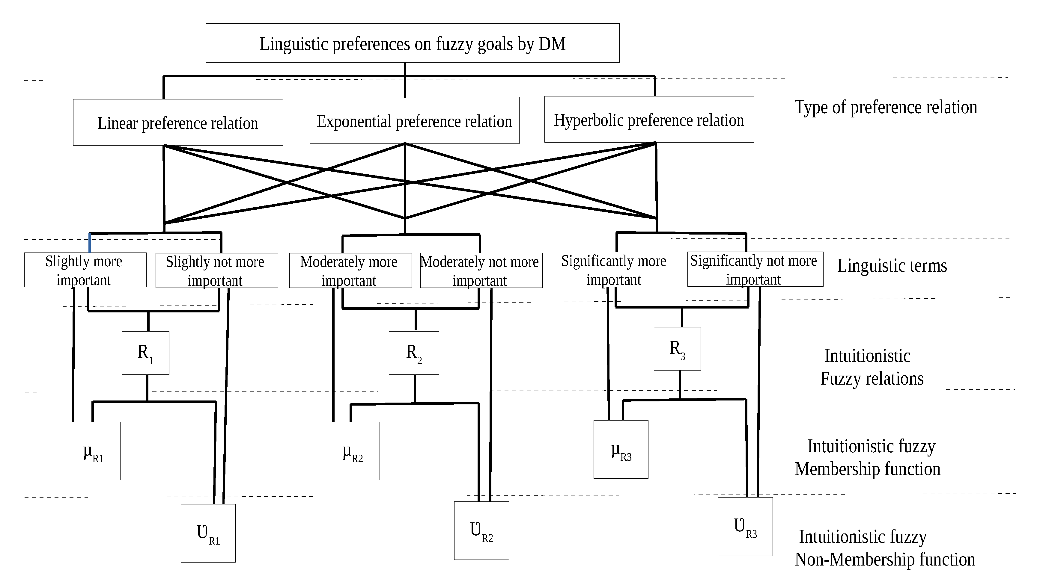
The hierarchy structure of the problem model is explained through Figure 1. It is divided into five sections as a type of preference relation, linguistic term, intuitionistic fuzzy relation, intuitionistic fuzzy membership function and intuitionistic fuzzy non-membership function. It explains that initially, the linguistic preference on fuzzy goals is assigned by the DM. It may be assigned as linear, exponential or hyperbolic preference relation. As the case is intuitionistic, these relations are further divided into three different categories of slightly, moderately and significantly more and not more important cases. The membership grade provides a satisfaction level of these relations. Whereas, the non-membership grade provides the satisfaction level of the opposite part of preference relation, i.e., not more important. The decision of the type of preference relation completely depends upon the type of real-life problem. The transform function for these preference relation is also defined in

Table 2. Linguistic relative preferences of goal k over l.

Linguistic Term	Fuzzy Relation	Intuitionistic Fuzzy		Transform Function
		Membership fn.	Non-Membership fn.
Slightly more important than	${\tilde{R}}_1$	${\mu }_{{\tilde{R}}_1}$	${\nu }_{{\tilde{R}}_1}$
Moderately more important than	${\tilde{R}}_2$	${\mu }_{{\tilde{R}}_2}$	${\nu }_{{\tilde{R}}_2}$	${\mu }_k\left(X\right)-{\mu }_l\left(X\right)$
Significantly more important than	${\tilde{R}}_3$	${\mu }_{{\tilde{R}}_3}$	${\nu }_{{\tilde{R}}_3}$	$\forall k,l\in (1\dots K)$

.

Before moving to the proposed FGP-IFPR, we shall first define the formulations for different membership and non-membership functions namely linear (L), exponential (E), and hyperbolic (H) for linguistic preference relations among different goals, which are to be maximized and minimized in order to achieve the importance among goals, respectively.

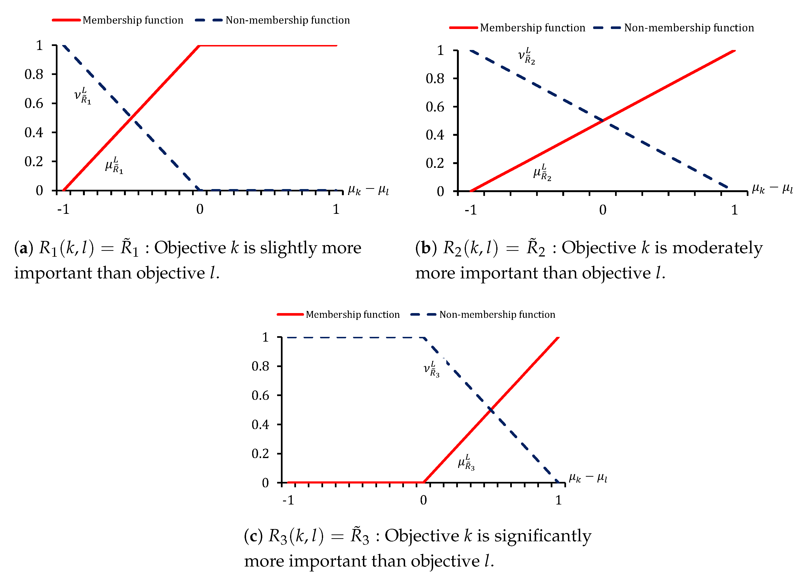
3.2.1. Linear Membership and Non-Membership Function

The linear membership function of an IFPR for each linguistic term can be defined as follows:

$$\begin{array}{cc}\hfill & {\mu }_{{\tilde{R}}_1(k,l)}^L=\left\{\begin{array}{cc}({\mu }_k-{\mu }_l+1),\hfill & \mathrm{if}-1\le {\mu }_k-{\mu }_l\le 0;\hfill \\ 1,\hfill & \mathrm{if}0\le {\mu }_k-{\mu }_l\le 1.\hfill \end{array}\right.\hfill \end{array}$$

(15a)

$$\begin{array}{cc}\hfill & {\mu }_{{\tilde{R}}_2(k,l)}^L=\left\{\begin{array}{cc}\left(\frac{{\mu }_k-{\mu }_l+1}{2}\right),\hfill & \mathrm{if}-1\le {\mu }_k-{\mu }_l\le 1;\hfill \end{array}\right.\hfill \end{array}$$

(15b)

$$\begin{array}{cc}\hfill & {\mu }_{{\tilde{R}}_3(k,l)}^L=\left\{\begin{array}{cc}0,\hfill & \mathrm{if}-1\le {\mu }_k-{\mu }_l\le 0;\hfill \\ ({\mu }_k-{\mu }_l),\hfill & \mathrm{if}0\le {\mu }_k-{\mu }_l\le 1.\hfill \end{array}\right.\hfill \end{array}$$

(15c)

where, ${\mu }_{{\tilde{R}}_1(k,l)}^L$, ${\mu }_{{\tilde{R}}_2(k,l)}^L$, and ${\mu }_{{\tilde{R}}_3(k,l)}^L$ represents the linear MFs of an IFPR for each linguistic term $\{{\tilde{R}}_1,{\tilde{R}}_2,{\tilde{R}}_3\}$.

The linear non-membership function for the IFPR for each linguistic term can be defined as follows:

$$\begin{array}{cc}\hfill & {\nu }_{{\tilde{R}}_1(k,l)}^L=\left\{\begin{array}{cc}-({\mu }_k-{\mu }_l),\hfill & \mathrm{if}-1\le {\mu }_k-{\mu }_l\le 0;\hfill \\ 0,\hfill & \mathrm{if}0\le {\mu }_k-{\mu }_l\le 1.\hfill \end{array}\right.\hfill \end{array}$$

(16a)

$$\begin{array}{cc}\hfill & {\nu }_{{\tilde{R}}_2(k,l)}^L=\left\{\begin{array}{cc}1,\hfill & \mathrm{if}-1\le {\mu }_k-{\mu }_l\le 0;\hfill \\ {\displaystyle \frac{1-({\mu }_k-{\mu }_l)}{2}},\hfill & \mathrm{if}0\le {\mu }_k-{\mu }_l\le 1.\hfill \end{array}\right.\hfill \end{array}$$

(16b)

$$\begin{array}{cc}\hfill & {\nu }_{{\tilde{R}}_3(k,l)}^L=\left\{\begin{array}{cc}1,\hfill & \mathrm{if}-1\le {\mu }_k-{\mu }_l\le 0;\hfill \\ 1-({\mu }_k-{\mu }_l),\hfill & \mathrm{if}0\le {\mu }_k-{\mu }_l\le 1.\hfill \end{array}\right.\hfill \end{array}$$

(16c)

where, ${\nu }_{{\tilde{R}}_1(k,l)}^L$, ${\nu }_{{\tilde{R}}_2(k,l)}^L$, and ${\nu }_{{\tilde{R}}_3(k,l)}^L$ represents the linear non-membership function of an IFPR for each linguistic term $\{{\tilde{R}}_1,{\tilde{R}}_2,{\tilde{R}}_3\}$. A pictorial demonstration of linear membership and non-membership function of IFPR ${\tilde{R}}_1$, ${\tilde{R}}_2$, and ${\tilde{R}}_3$ are shown in Figure 2.

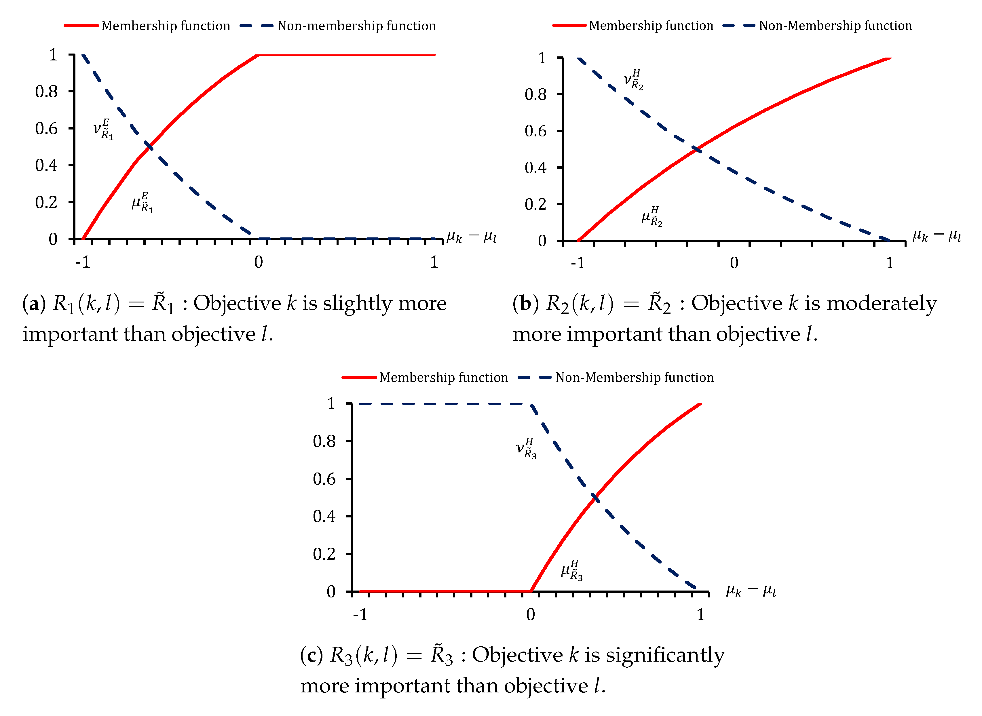
3.2.2. Exponential Membership and Non-Membership Function

The exponential membership function of an IFPR for each linguistic term can be defined as follows:

$$\begin{array}{cc}\hfill & {\mu }_{{\tilde{R}}_1(k,l)}^E=\left\{\begin{array}{cc}{\displaystyle \frac{1-e^{-s*({\mu }_k-{\mu }_l+1)}}{1-e^{-s}}},\hfill & \mathrm{if}-1\le {\mu }_k-{\mu }_l\le 0;\hfill \\ 1,\hfill & \mathrm{if}0\le {\mu }_k-{\mu }_l\le 1.\hfill \end{array}\right.\hfill \end{array}$$

(17a)

$$\begin{array}{cc}\hfill & {\mu }_{{\tilde{R}}_2(k,l)}^E=\left\{\begin{array}{cc}{\displaystyle \frac{1-e^{-s*(\frac{{\mu }_k-{\mu }_l+1}{2})}}{1-e^{-s}}},\hfill & \mathrm{if}-1\le {\mu }_k-{\mu }_l\le 1;\hfill \end{array}\right.\hfill \end{array}$$

(17b)

$$\begin{array}{cc}\hfill & {\mu }_{{\tilde{R}}_3(k,l)}^E=\left\{\begin{array}{cc}0,\hfill & \mathrm{if}-1\le {\mu }_k-{\mu }_l\le 0;\hfill \\ {\displaystyle \frac{1-e^{-s*({\mu }_k-{\mu }_l)}}{1-e^{-s}}},\hfill & \mathrm{if}0\le {\mu }_k-{\mu }_l\le 1.\hfill \end{array}\right.\hfill \end{array}$$

(17c)

where, ${\mu }_{{\tilde{R}}_1(k,l)}^E$, ${\mu }_{{\tilde{R}}_2(k,l)}^E$, and ${\mu }_{{\tilde{R}}_3(k,l)}^E$ represents the exponential membership function of an IFPR for each linguistic term $\{{\tilde{R}}_1,{\tilde{R}}_2,{\tilde{R}}_3\}$. Additionally, s is the measurement of grades of fuzziness and defined by the decision makers according to the ambiguity of the relations.

The exponential non-membership function of an IFPR for each linguistic term can be defined as follows:

$$\begin{array}{cc}\hfill & {\nu }_{{\tilde{R}}_1(k,l)}^E=\left\{\begin{array}{cc}{\displaystyle \frac{e^{-s*({\mu }_k-{\mu }_l+1)}-e^{-s}}{1-e^{-s}}},\hfill & \mathrm{if}-1\le {\mu }_k-{\mu }_l\le 0;\hfill \\ 0,\hfill & \mathrm{if}0\le {\mu }_k-{\mu }_l\le 1.\hfill \end{array}\right.\hfill \end{array}$$

(18a)

$$\begin{array}{cc}\hfill & {\nu }_{{\tilde{R}}_2(k,l)}^E=\left\{\begin{array}{cc}{\displaystyle \frac{e^{-s*\left(\frac{{\mu }_k-{\mu }_l+1}{2}\right)}-e^{-s}}{1-e^{-s}}},\hfill & \mathrm{if}-1\le {\mu }_k-{\mu }_l\le 1;\hfill \end{array}\right.\hfill \end{array}$$

(18b)

$$\begin{array}{cc}\hfill & {\nu }_{{\tilde{R}}_3(k,l)}^E=\left\{\begin{array}{cc}1,\hfill & \mathrm{if}-1\le {\mu }_k-{\mu }_l\le 0;\hfill \\ {\displaystyle \frac{e^{-s*({\mu }_k-{\mu }_l)}-e^{-s}}{1-e^{-s}}},\hfill & \mathrm{if}0\le {\mu }_k-{\mu }_l\le 1.\hfill \end{array}\right.\hfill \end{array}$$

(18c)

where ${\nu }_{{\tilde{R}}_1(k,l)}^E$, ${\nu }_{{\tilde{R}}_2(k,l)}^E$, and ${\nu }_{{\tilde{R}}_3(k,l)}^E$ represents the exponential non-membership function of an IFPR for each linguistic term $\{{\tilde{R}}_1,{\tilde{R}}_2,{\tilde{R}}_3\}$. A pictorial demonstration of exponential membership and non-membership function of IFPRs ${\tilde{R}}_1$, ${\tilde{R}}_2$, and ${\tilde{R}}_3$ are shown in Figure 3.

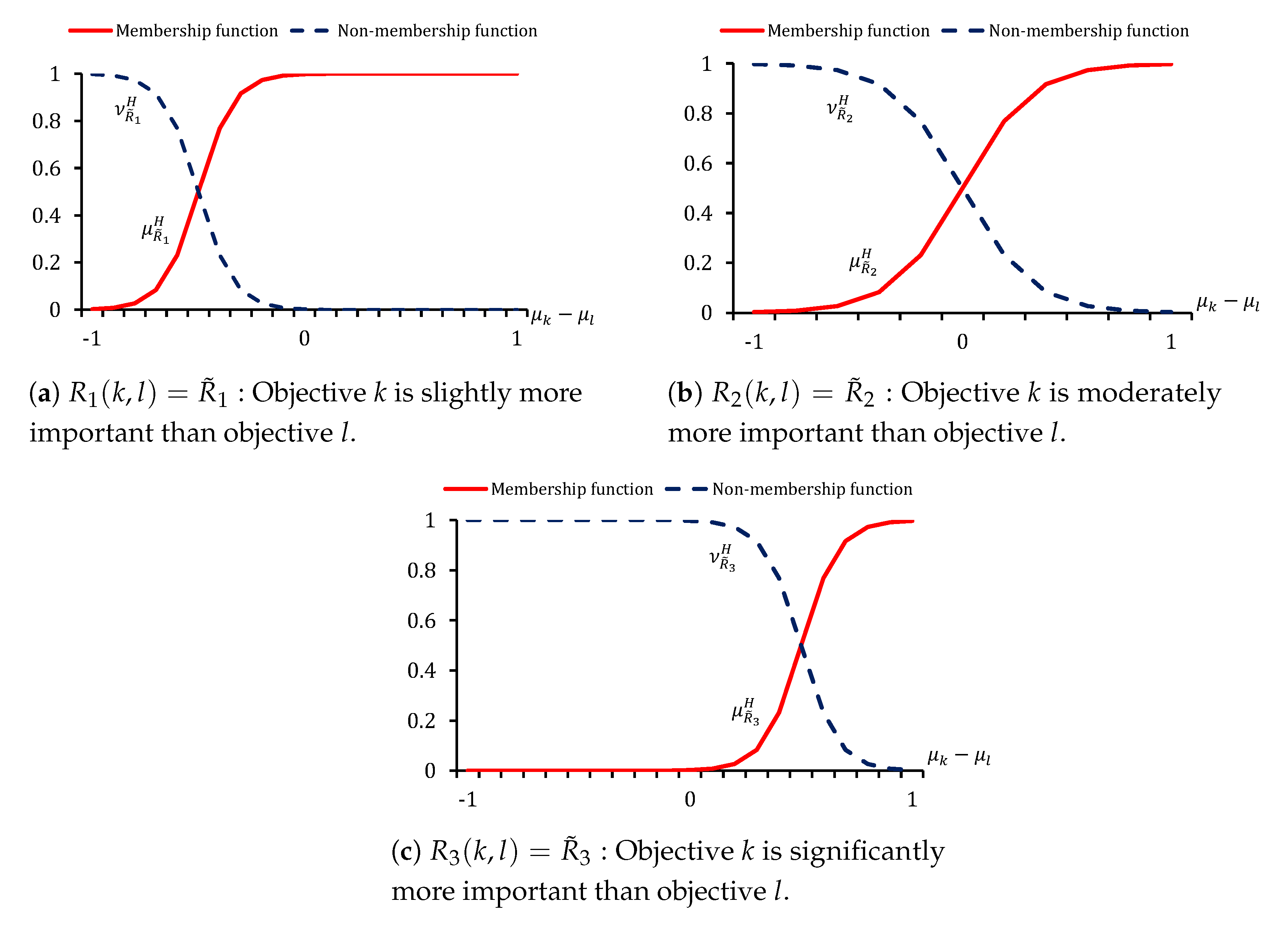
3.2.3. Hyperbolic Membership and Non-Membership Function

The hyperbolic membership function of an IFPR for each linguistic term can be defined as follows:

$$\begin{array}{cc}\hfill & {\mu }_{{\tilde{R}}_1(k,l)}^H=\left\{\begin{array}{cc}{\displaystyle \frac{e^{3+6({\mu }_k-{\mu }_l)}}{e^{-\left(3+6({\mu }_k-{\mu }_l)\right)}+e^{3+6({\mu }_k-{\mu }_l)}}}+{\displaystyle \frac{e^{-3}}{e^{-3}+e^3}},\hfill & \mathrm{if}-1\le {\mu }_k-{\mu }_l\le 0;\hfill \\ 1,\hfill & \mathrm{if}0\le {\mu }_k-{\mu }_l\le 1.\hfill \end{array}\right.\hfill \end{array}$$

(19a)

$$\begin{array}{cc}\hfill & {\mu }_{{\tilde{R}}_2(k,l)}^H=\left\{\begin{array}{cc}{\displaystyle \frac{e^{3({\mu }_k-{\mu }_l)}}{e^{-3({\mu }_k-{\mu }_l)}+e^{3({\mu }_k-{\mu }_l)}}},\hfill & \mathrm{if}-1\le {\mu }_k-{\mu }_l\le 1;\hfill \end{array}\right.\hfill \end{array}$$

(19b)

$$\begin{array}{cc}\hfill & {\mu }_{{\tilde{R}}_3(k,l)}^H=\left\{\begin{array}{cc}0,\hfill & \mathrm{if}-1\le {\mu }_k-{\mu }_l\le 0;\hfill \\ {\displaystyle \frac{e^{-3+6({\mu }_k-{\mu }_l)}}{e^{3-6({\mu }_k-{\mu }_l)}+e^{-3+6({\mu }_k-{\mu }_l)}}}-{\displaystyle \frac{e^{-3}}{e^{-3}+e^3}},\hfill & \mathrm{if}0\le {\mu }_k-{\mu }_l\le 1.\hfill \end{array}\right.\hfill \end{array}$$

(19c)

where, ${\mu }_{{\tilde{R}}_1(k,l)}^H$, ${\mu }_{{\tilde{R}}_2(k,l)}^H$, and ${\mu }_{{\tilde{R}}_3(k,l)}^H$ represents the hyperbolic membership function of an IFPR for each linguistic term $\{{\tilde{R}}_1,{\tilde{R}}_2,{\tilde{R}}_3\}$.

The hyperbolic non-membership function of an IFPR for each linguistic term can be defined as follows:

$$\begin{array}{cc}\hfill & {\nu }_{{\tilde{R}}_1(k,l)}^H=\left\{\begin{array}{cc}{\displaystyle \frac{e^{-\left(3+6({\mu }_k-{\mu }_l)\right)}}{e^{-\left(3+6({\mu }_k-{\mu }_l)\right)}+e^{3+6({\mu }_k-{\mu }_l)}}}-{\displaystyle \frac{e^{-3}}{e^{-3}+e^3}},\hfill & \mathrm{if}-1\le {\mu }_k-{\mu }_l\le 0;\hfill \\ 0,\hfill & \mathrm{if}0\le {\mu }_k-{\mu }_l\le 1.\hfill \end{array}\right.\hfill \end{array}$$

(20a)

$$\begin{array}{cc}\hfill & {\nu }_{{\tilde{R}}_2(k,l)}^H=\left\{\begin{array}{cc}{\displaystyle \frac{e^{-3({\mu }_k-{\mu }_l)}}{e^{-3({\mu }_k-{\mu }_l)}+e^{3({\mu }_k-{\mu }_l)}}},\hfill & \mathrm{if}-1\le {\mu }_k-{\mu }_l\le 1;\hfill \end{array}\right.\hfill \end{array}$$

(20b)

$$\begin{array}{cc}\hfill & {\nu }_{{\tilde{R}}_3(k,l)}^H=\left\{\begin{array}{cc}1,\hfill & \mathrm{if}-1\le {\mu }_k-{\mu }_l\le 0;\hfill \\ {\displaystyle \frac{e^{3-6({\mu }_k-{\mu }_l)}}{e^{3-6({\mu }_k-{\mu }_l)}+e^{-3+6({\mu }_k-{\mu }_l)}}}+{\displaystyle \frac{e^{-3}}{e^{-3}+e^3}},\hfill & \mathrm{if}0\le {\mu }_k-{\mu }_l\le 1.\hfill \end{array}\right.\hfill \end{array}$$

(20c)

here, ${\nu }_{{\tilde{R}}_1(k,l)}^H$, ${\nu }_{{\tilde{R}}_2(k,l)}^H$, and ${\nu }_{{\tilde{R}}_3(k,l)}^H$ represents the exponential non-membership function of an IFPR for each linguistic term $\{{\tilde{R}}_1,{\tilde{R}}_2,{\tilde{R}}_3\}$. A pictorial demonstration of hyperbolic membership and non-membership function of IFPRs ${\tilde{R}}_1$, ${\tilde{R}}_2$, and ${\tilde{R}}_3$ are shown in Figure 4.

It is to be mentioned that the membership and non-membership function of IFPRs are defined over the transform function ${\mu }_k-{\mu }_l$ where k is not equal to l. k and l, both represents the index of MF of objective function, see Khalili-Damghani et al. [55] and Khalili-Damghani et al. [56]. The membership functions of IFPRs have to be maximizied, whereas, non-membership functions minimized in order to achieve the relative importance among the intuitionistic fuzzy goals.

3.3. Proposed FGP-IFPR Model

Aköz and Petrovic [31] defined the achievement function as a convex combination of the sum of individual membership function of fuzzy goals and the sum of satisfaction degrees of the imprecise linguistic importance relations but here, for FGP-IFPR, we define the achievement function as a convex combination of the sum of individual membership function of fuzzy goals and the sum of score functions of the imprecise linguistic importance relations.

In order to achieve these fuzzy goals, we define score function

$$S_{{\tilde{R}}_i(k,l)}^A=({\mu }_{{\tilde{R}}_i(k,l)}^A-{\nu }_{{\tilde{R}}_i(k,l)}^A),\forall i=1,2and3,$$

(21)

Let $b_{kl},\forall k,l=1,2,\dots ,K$ where $k\ne l$; be a binary variable, taking value 1 if there is an importance relation defined between the goal $Z_k$ and $Z_l$, and 0 otherwise. The lower and upper tolerance limit for each fuzzy goal is represented by $t_k$ and $u_k$ respectively. So, the proposed model with new achievement function and with weight $\alpha$ in intuitionistic fuzzy environment is formulated as follows:   

$$\begin{array}{cc}\hfill \mathrm{Maximize}& Z=\alpha (\sum _{k=1}^K{\mu }_k)+(1-\alpha )(\sum _{k=1}^K\sum _{l=1}^K{b}_{k,l}{S}_{{\tilde{R}}_i(k,l)}^A)\hfill \end{array}$$

(22a)

$$\begin{array}{cc}\hfill \mathrm{subject}\mathrm{to},& {\mu }_k={\displaystyle \frac{Z_k\left(x\right)-t_k}{a_k-t_k}},\left(Maximizationtypegoal\right)\hfill \end{array}$$

(22b)

$$\begin{array}{cc}\hfill & {\mu }_k={\displaystyle \frac{u_k-Z_k\left(x\right)}{u_k-a_k}},\left(Minimizationtypegoal\right)\hfill \end{array}$$

(22c)

$$\begin{array}{cc}\hfill & 0\le {\mu }_k\le 1\hfill \end{array}$$

(22d)

$$\begin{array}{cc}\hfill & {\mu }_{{\tilde{R}}_i(k,l)}^A\ge {\mu }_{{\tilde{R}}_i(k,l)}\hfill \end{array}$$

(22e)

$$\begin{array}{cc}\hfill & {\nu }_{{\tilde{R}}_i(k,l)}^A\le {\nu }_{{\tilde{R}}_i(k,l)}\hfill \end{array}$$

(22f)

$$\begin{array}{cc}\hfill & S_{{\tilde{R}}_i(k,l)}^A=({\mu }_{{\tilde{R}}_i(k,l)}^A-{\nu }_{{\tilde{R}}_i(k,l)}^A)\hfill \end{array}$$

(22g)

$$\begin{array}{cc}\hfill & {\mu }_{{\tilde{R}}_i(k,l)}^A\ge {\nu }_{{\tilde{R}}_i(k,l)}^A\hfill \end{array}$$

(22h)

$$\begin{array}{cc}\hfill & 0\le {\mu }_{{\tilde{R}}_i(k,l)}^A+{\nu }_{{\tilde{R}}_i(k,l)}^A\le 1\hfill \end{array}$$

(22i)

$$\begin{array}{cc}\hfill & 0\le {\mu }_{\tilde{R}(k,l)}^A\le 1,0\le {\nu }_{{\tilde{R}}_i(k,l)}^A\le 1\forall b_{kl}=1or0\hfill \end{array}$$

(22j)

$$\begin{array}{cc}\hfill & Ax\le b,x\ge 0\hfill \end{array}$$

(22k)

$$\begin{array}{cc}\hfill & \forall i=1,2and3;k,l=1,2,\dots ,Kwherek\ne l.\hfill \end{array}$$

(22l)

where superscript $A=(L,E,andH)$ represents the type of membership functions i.e., linear, exponential and hyperbolic used to express the satisfactory degree of decision makers respectively. ${\mu }_{{\tilde{R}}_i(k,l)}^A$ and ${\nu }_{{\tilde{R}}_i(k,l)}^A,\forall A=linear,exponential\mathrm{and}hyperbolic$; represents the type of membership and non-membership function used by the decision makers and $i=1,2$ and $3$ represents the type of linguistic preference relation among different fuzzy goals. ${\mu }_k$ represents the membership grade for kth objective function or goal.

4. Solution Approach

The approach to solving the proposed FGP-IFPR models is a composition of several steps. The first step is to formulate the crisp model of the problem with all the goal functions. After that, for determining the tolerance and aspiration values of the respective goal functions, either the crisp model is solved for each objective function or the decision-maker may provide it. The obtained solution should be feasible and optimal. Take the optimum value of objective functions as the target aspiration value. Determine then all of the objective function values for the solution obtained. This step will give us a payoff table (values of extreme solutions), and aspiration, including tolerance level values. Formulate all membership grades for objective functions which are fuzzy goals. Create the transform function for preferential linguistic relationships by using objective functions membership grades. Establish the intuitionistic fuzzy preferential linguistic relationships between different objective functions, and formulate the intuitionistic fuzzy membership and non-membership grades functions. Form the desired intuitionistic fuzzy preference relationship function (IFPR) among the fuzzy goals, it can be either linear or exponential or hyperbolic function. Define the score function by taking the difference of membership and non-membership function of each IFPRs. Now, formulate the FGP-IFPR models for the problem, as detailed in the section above. Solve the formulation using any optimization software packages. We have used the NEOS server online facility provided by Wisconsin Institutes for Discovery at the University of Wisconsin in Madison for solving optimization problems, and AMPL (Fourer et al. [63]) for mathematical modeling of the issues.

In this paper, the obtained FGP-IFPR model has been modeled in AMPL language (Fourer et al. [63]) and solved using solvers available on NEOS server online facility provided by Wisconsin Institutes for Discovery at the University of Wisconsin in Madison for solving optimization problems, see Gropp, W. Moré [64], Czyzyk et al. [65], Dolan [66] and Server [67]. As the results are obtained, we need to investigate the feasibility of solutions. If the result is infeasible, rest the aspiration and tolerance conditions and restart, if not, offer the answer to the experts. The step by step procedure of the solution approach is presented in Algorithm 1 and Figure 5 shows the flow diagram.

Algorithm 1 Solution approach

1: Input: Data and parametric values of problem. 2: Output: Optimal solution. 3: Formulate the crisp multi-objective programming problem. 4: Consider K-single objective optimization problems and determine the individual optima. 5: if Aspiration values are not known then 6:     Find the optimal values of each single objective optimization problem. 7: Evaluate the membership function for each fuzzy goals. 8: Define the linguistic preference relations among the different goals by using membership and non-membership functions via choosing linear or non-linear function. 9: Calculate the score function by considering the difference of membership and non-membership function for each fuzzy preference relation. 10: Formulate the FGP-IFPR model with their aspiration values. 11: Apply the optimization toolbox for finding the optimal solutions. 12: Stop and present the solution obtained to the decision maker.

5. Experimental Study

In order to validate the proposed models, we considered two examples. The first example was a numerical example and second one was a banking application problem. The problems were modeled as the proposed FGP-IFPR using all of the linear, exponential, and hyperbolic membership functions.

5.1. Example 1

In this numerical example, used by Chen and Tsai [30], Aköz and Petrovic [31], Cheng [33] and Arenas-Parra et al. [44], we had to find best solution $x=(x_1,x_2,x_3,x_4)$ for the following multi-objective mathematical programming problem.

$$\begin{array}{cc}\hfill \mathrm{Goal}1:& 4x_1+2x_2+8x_3+x_4\le 35\hfill \end{array}$$

(23a)

$$\begin{array}{cc}\hfill \mathrm{Goal}2:& 4x_1+7x_2+6x_3+2x_4\ge 100\hfill \end{array}$$

(23b)

$$\begin{array}{cc}\hfill \mathrm{Goal}3:& x_1-6x_2+5x_3+10x_4\ge 120\hfill \end{array}$$

(23c)

$$\begin{array}{cc}\hfill \mathrm{Goal}4:& 5x_1+3x_2+2x_4\ge 70\hfill \end{array}$$

(23d)

$$\begin{array}{cc}\hfill \mathrm{Goal}5:& 4x_1+4x_2+4x_3\ge 40\hfill \end{array}$$

(23e)

$$\begin{array}{cc}\hfill \mathrm{subject}\mathrm{to}& 7x_1+5x_2+3x_3+2x_4\le 98\hfill \end{array}$$

(23f)

$$\begin{array}{cc}\hfill & 7x_1+x_2+2x_3+6x_4\le 117\hfill \end{array}$$

(23g)

$$\begin{array}{cc}\hfill & x_1+x_2+2x_3+6x_4\le 130\hfill \end{array}$$

(23h)

$$\begin{array}{cc}\hfill & 9x_1+x_2+6x_4\le 105\hfill \end{array}$$

(23i)

$$\begin{array}{cc}\hfill & x_i\ge 0,i=1,\dots ,4.\hfill \end{array}$$

(23j)

Here, we had five objectives as Goal-1, Goal-2, Goal-3, Goal-4, and Goal-5. The fuzzy preference relations among these objectives (goals) were given as follows:

• Goal-1 is moderately more important than Goal-2 (${\mu }_{12}$).
• Goal-2 is moderately more important than Goal-4 (${\mu }_{24}$).
• Goal-2 is moderately more important than Goal-5 (${\mu }_{25}$).
• Goal-3 is moderately more important than Goal-2 (${\mu }_{32}$).

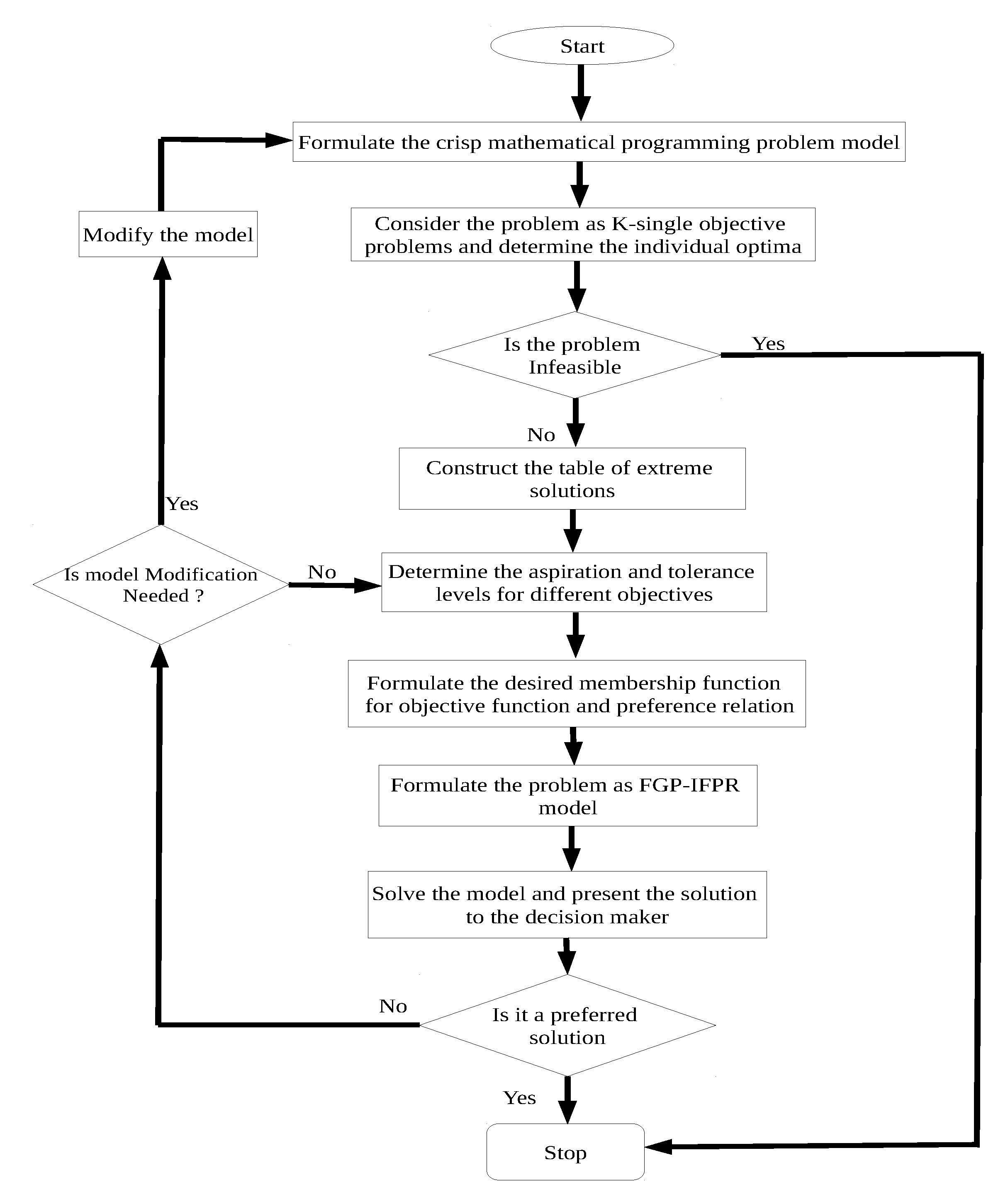
Now, the problem has been solved using solution approach of Algorithm 1 by applying proposed FGP-IFPR models and results were obtained.

5.2. Solution Steps for Example 1

The solution steps are summarized as follows.

Step-1 Start with given multi-objective programming problem as given in Equations (23a)–(23j).

Step-2 Formulate the problem as five single objective models (based on the respective goals). All the five optimization problems are solved for finding the best and worst values of goals. The decision maker can provide the aspiration values as per choice or determine it based on individual solution of the problem models.

Step-3 For this multi objective problem, the tolerance limits are provided. The upper limit for minimization type fuzzy goal $Z_1$ is $u_1=55$, the lower limits for maximization type fuzzy goals $Z_2$, $Z_3$, $Z_4$ and $Z_5$ are $t_2=40$, $t_3=70$, $t_4=30$ and $t_5=10$, respectively, with $a_k$ as their corresponding aspiration levels.

Step-4 The membership function (${\mu }_k$) for each objective function $Z_k$ is modeled using Equations (7) and (8) as follows:

$${\mu }_1=\frac{(55-Z_1)}{(55-35)};{\mu }_2=\frac{(Z_2-40)}{(100-40)};{\mu }_3=\frac{(Z_3-70)}{(120-70)};{\mu }_4=\frac{(Z_4-30)}{(70-30)};{\mu }_5=\frac{(Z_5-10)}{(40-10)}.$$

Step-5 The intuitionistic fuzzy functions for the preference relations are formulated and presented in this step. Suppose, ${\mu }_{12}$, ${\mu }_{24}$, ${\mu }_{25}$, and ${\mu }_{32}$ are the intuitionistic fuzzy membership function and ${\nu }_{12}$, ${\nu }_{24}$, ${\nu }_{25}$, and ${\nu }_{32}$ are intuitionistic fuzzy non-membership function with respect to the linguistic preference relations as given in problem definition. Thus, the linear membership function and non-membership function formulation for each preference relation using Equations (15a)–(15c) and Equations (16a)–(16c) are as:

$${\mu }_{12}=\frac{({\mu }_1-{\mu }_2+1)}{2};{\mu }_{24}=\frac{({\mu }_2-{\mu }_4+1)}{2};{\mu }_{25}=\frac{({\mu }_2-{\mu }_5+1)}{2};{\mu }_{32}=\frac{({\mu }_3-{\mu }_2+1)}{2}.$$

$$v_{12}=\frac{(1-{\mu }_1+{\mu }_2)}{2};v_{24}=\frac{(1-{\mu }_2+{\mu }_4)}{2};v_{25}=\frac{(1-{\mu }_2+{\mu }_5)}{2};v_{32}=\frac{(1-{\mu }_3+{\mu }_2)}{2}.$$

The exponential membership function and non-membership function formulation for each preference relation using Equations (17a)–(17c) and Equations (18a)–(18c) are as:

$${\mu }_{12}=\frac{(1-e^{-s.({\mu }_1-{\mu }_2+1)/2})}{(1-e^{-s})};{\mu }_{24}=\frac{(1-e^{-s.({\mu }_2-{\mu }_4+1)/2})}{(1-e^{-s})};$$

$${\mu }_{25}=\frac{(1-e^{-s.({\mu }_2-{\mu }_5+1)/2})}{(1-e^{-s})};{\mu }_{32}=\frac{(1-e^{-s.({\mu }_3-{\mu }_2+1)/2})}{(1-e^{-s})}.$$

$$v_{12}=\frac{(e^{-s.({\mu }_1-{\mu }_2+1)/2}-e^{-s})}{(1-e^{-s})};v_{24}=\frac{(e^{-s.({\mu }_2-{\mu }_4+1)/2}-e^{-s})}{(1-e^{-s})};$$

$$v_{25}=\frac{(e^{-s.({\mu }_2-{\mu }_5+1)/2}-e^{(-s)})}{(1-e^{-s})};v_{32}=\frac{(e^{-s.({\mu }_3-{\mu }_2+1)/2}-e^{-s})}{(1-e^{-s})}.$$

The hyperbolic membership function and non-membership function formulation for each preference relation using Equations (19a)–(19c) and Equations (20a)–(20c) are as:

$${\mu }_{12}={\displaystyle \frac{e^{3({\mu }_1-{\mu }_2)}}{e^{-3({\mu }_1-{\mu }_2)}+e^{3({\mu }_1-{\mu }_2)}}};{\mu }_{24}={\displaystyle \frac{e^{3({\mu }_2-{\mu }_4)}}{e^{-3({\mu }_2-{\mu }_4)}+e^{3({\mu }_2-{\mu }_4)}}};$$

$${\mu }_{25}={\displaystyle \frac{e^{3({\mu }_2-{\mu }_5)}}{e^{-3({\mu }_2-{\mu }_5)}+e^{3({\mu }_2-{\mu }_5)}}};{\mu }_{32}={\displaystyle \frac{e^{3({\mu }_3-{\mu }_2)}}{e^{-3({\mu }_3-{\mu }_2)}+e^{3({\mu }_3-{\mu }_2)}}}].$$

$$v_{12}={\displaystyle \frac{e^{-3({\mu }_1-{\mu }_2)}}{e^{-3({\mu }_1-{\mu }_2)}+e^{3({\mu }_1-{\mu }_2)}}};v_{24}={\displaystyle \frac{e^{-3({\mu }_2-{\mu }_4)}}{e^{-3({\mu }_2-{\mu }_4)}+e^{3({\mu }_2-{\mu }_4)}}};$$

$$v_{25}={\displaystyle \frac{e^{-3({\mu }_2-{\mu }_5)}}{e^{-3({\mu }_2-{\mu }_5)}+e^{3({\mu }_2-{\mu }_5)}}};v_{32}={\displaystyle \frac{e^{-3({\mu }_3-{\mu }_2)}}{e^{-3({\mu }_3-{\mu }_2)}+e^{3({\mu }_3-{\mu }_2)}}}.$$

Step-6 Problem formulations: The FGP-IFPR model of numerical Example-1 is formulated using preference relation functions.

We apply three different kinds of intuitionistic fuzzy functions for preference relations, namely, linear, exponential, and hyperbolic, so there are three different formulations.

Formulation I: FGP-IFPR for linear.

$$\begin{array}{cc}\hfill \mathrm{Maximize}& \alpha .({\mu }_1+{\mu }_2+{\mu }_3+{\mu }_4+{\mu }_5)+(1-\alpha ).(S_{12}+S_{24}+S_{25}+S_{32})\hfill \\ \hfill \mathrm{subject}\mathrm{to},& \hfill \end{array}$$

(24a)

$$\begin{array}{cc}\hfill & {\mu }_{12}\le \frac{({\mu }_1-{\mu }_2+1)}{2};{\mu }_{24}\le \frac{({\mu }_2-{\mu }_4+1)}{2};{\mu }_{25}\le \frac{({\mu }_2-{\mu }_5+1)}{2};{\mu }_{32}\le \frac{({\mu }_3-{\mu }_2+1)}{2};\hfill \end{array}$$

(24b)

$$\begin{array}{cc}\hfill & v_{12}\ge \frac{(1-{\mu }_1+{\mu }_2)}{2};v_{24}\ge \frac{(1-{\mu }_2+{\mu }_4)}{2};v_{25}\ge \frac{(1-{\mu }_2+{\mu }_5)}{2};v_{32}\ge \frac{(1-{\mu }_3+{\mu }_2)}{2};\hfill \end{array}$$

(24c)

$$\begin{array}{cc}\hfill & S_{12}={\mu }_{12}-v_{12};S_{24}={\mu }_{24}-v_{24};S_{25}={\mu }_{25}-v_{25};S_{32}={\mu }_{32}-v_{32}\hfill \end{array}$$

(24d)

$$\begin{array}{cc}\hfill & {\mu }_1=\frac{(55-Z_1)}{(55-35)};{\mu }_2=\frac{(Z_2-40)}{(100-40)};{\mu }_3=\frac{(Z_3-70)}{(120-70)};{\mu }_4=\frac{(Z_4-30)}{(70-30)};{\mu }_5=\frac{(Z_5-10)}{(40-10)};\hfill \end{array}$$

(24e)

$$\begin{array}{cc}\hfill & 0\le {\mu }_1\le 1;0\le {\mu }_2\le 1;0\le {\mu }_3\le 1;0\le {\mu }_4\le 1;0\le {\mu }_5\le 1\hfill \end{array}$$

(24f)

$$\begin{array}{cc}\hfill & 1\ge {\mu }_{12}\ge v_{12}\ge 0;1\ge {\mu }_{24}\ge v_{24}\ge 0;1\ge {\mu }_{25}\ge v_{25}\ge 0;1\ge {\mu }_{32}\ge v_{32}\ge 0;\hfill \end{array}$$

(24g)

$$\begin{array}{cc}\hfill & 0\le {\mu }_{12}+v_{12}\le 1;0\le {\mu }_{24}+v_{24}\le 1;0\le {\mu }_{25}+v_{25}\le 1;0\le {\mu }_{32}+v_{32}\le 1;\hfill \end{array}$$

(24h)

Equations (23f)–(23j)

Formulation II: FGP-IFPR for exponential.

$$\begin{array}{cc}\hfill \mathrm{Maximize}& \alpha .({\mu }_1+{\mu }_2+{\mu }_3+{\mu }_4+{\mu }_5)+(1-\alpha ).(S_{12}+S_{24}+S_{25}+S_{32})\hfill \\ \hfill \mathrm{subject}\mathrm{to},& \hfill \end{array}$$

(25a)

$$\begin{array}{cc}\hfill & {\mu }_{12}\le \frac{(1-e^{-s.({\mu }_1-{\mu }_2+1)/2})}{(1-e^{-s})};{\mu }_{24}\le \frac{(1-e^{-s.({\mu }_2-{\mu }_4+1)/2})}{(1-e^{-s})};\hfill \end{array}$$

(25b)

$$\begin{array}{cc}\hfill & {\mu }_{25}\le \frac{(1-e^{-s.({\mu }_2-{\mu }_5+1)/2})}{(1-e^{-s})};{\mu }_{32}\le \frac{(1-e^{-s.({\mu }_3-{\mu }_2+1)/2})}{(1-e^{-s})};\hfill \end{array}$$

(25c)

$$\begin{array}{cc}\hfill & v_{12}\ge \frac{(e^{-s.({\mu }_1-{\mu }_2+1)/2}-e^{-s})}{(1-e^{-s})};v_{24}\ge \frac{(e^{-s.({\mu }_2-{\mu }_4+1)/2}-e^{-s})}{(1-e^{-s})};\hfill \end{array}$$

(25d)

$$\begin{array}{cc}\hfill & v_{25}\ge \frac{(e^{-s.({\mu }_2-{\mu }_5+1)/2}-e^{(-s)})}{(1-e^{-s})};v_{32}\ge \frac{(e^{-s.({\mu }_3-{\mu }_2+1)/2}-e^{-s})}{(1-e^{-s})}\hfill \end{array}$$

(25e)

Equations (24d)–(24h)

Equations (23f)–(23j)

Formulation III: FGP-IFPR for hyperbolic.

$$\begin{array}{cc}\hfill \mathrm{Maximize}& \alpha .({\mu }_1+{\mu }_2+{\mu }_3+{\mu }_4+{\mu }_5)+(1-\alpha ).(S_{12}+S_{24}+S_{25}+S_{32})\hfill \\ \hfill \mathrm{subject}\mathrm{to},& \hfill \end{array}$$

(26a)

$$\begin{array}{cc}\hfill & {\mu }_{12}\le {\displaystyle \frac{e^{3({\mu }_1-{\mu }_2)}}{e^{-3({\mu }_1-{\mu }_2)}+e^{3({\mu }_1-{\mu }_2)}}};{\mu }_{24}\le {\displaystyle \frac{e^{3({\mu }_2-{\mu }_4)}}{e^{-3({\mu }_2-{\mu }_4)}+e^{3({\mu }_2-{\mu }_4)}}};\hfill \end{array}$$

(26b)

$$\begin{array}{cc}\hfill & {\mu }_{25}\le {\displaystyle \frac{e^{3({\mu }_2-{\mu }_5)}}{e^{-3({\mu }_2-{\mu }_5)}+e^{3({\mu }_2-{\mu }_5)}}};{\mu }_{32}\le {\displaystyle \frac{e^{3({\mu }_3-{\mu }_2)}}{e^{-3({\mu }_3-{\mu }_2)}+e^{3({\mu }_3-{\mu }_2)}}};\hfill \end{array}$$

(26c)

$$\begin{array}{cc}\hfill & v_{12}\ge {\displaystyle \frac{e^{-3({\mu }_1-{\mu }_2)}}{e^{-3({\mu }_1-{\mu }_2)}+e^{3({\mu }_1-{\mu }_2)}}};v_{24}\ge {\displaystyle \frac{e^{-3({\mu }_2-{\mu }_4)}}{e^{-3({\mu }_2-{\mu }_4)}+e^{3({\mu }_2-{\mu }_4)}}};\hfill \end{array}$$

(26d)

$$\begin{array}{cc}\hfill & v_{25}\ge {\displaystyle \frac{e^{-3({\mu }_2-{\mu }_5)}}{e^{-3({\mu }_2-{\mu }_5)}+e^{3({\mu }_2-{\mu }_5)}}};v_{32}\ge {\displaystyle \frac{e^{-3({\mu }_3-{\mu }_2)}}{e^{-3({\mu }_3-{\mu }_2)}+e^{3({\mu }_3-{\mu }_2)}}};\hfill \end{array}$$

(26e)

Equations (24d)–(24h)

Equations (23f)–(23j)

Step-7 Now, we solve the above FGP-IFPR models of example 1 using any linear and non linear optimization solver and software.

Step-8 Stop, the optimal and feasible solution is obtained.

Results and Discussion for Example 1

The problem consisting of five multiple objectives was modelled and solved. It provided a feasible and optimal result. To get a more detailed nature of three FGP-IFPR models, the results were evaluated for $\alpha =0,0.1,0.2,0.3,0.4,0.5,0.6,0.7,0.8,0.9\mathrm{and}1$.

The results obtained on solving are presented in

Table 3. Result values for preference membership, non-membership grades and score function of proposed FGP-IFPR for Example 1.

Formulation	$\mathit{\alpha }$	${\mathit{\mu }}_{12}$	${\mathit{\mu }}_{24}$	${\mathit{\mu }}_{25}$	${\mathit{\mu }}_{32}$	$\sum {\mathit{\mu }}_{{\mathit{R}}_{\mathit{i}}}(\mathit{k},\mathit{l})$	${\mathit{\nu }}_{12}$	${\mathit{\nu }}_{24}$	${\mathit{\nu }}_{25}$	${\mathit{v}}_{32}$	$\sum {\mathit{\nu }}_{{\mathit{R}}_{\mathit{i}}}(\mathit{k},\mathit{l})$	$\sum {\mathit{S}}_{{\mathit{R}}_{\mathit{i}}}(\mathit{k},\mathit{l})$
I:FGP-IFPR	0.0	0.7795	0.5954	0.7795	0.500	2.6545	0.2204	0.4045	0.2204	0.5000	1.3453	1.3091
for Linear	0.1	0.7795	0.5954	0.7795	0.5000	2.6545	0.2204	0.4045	0.2204	0.5000	1.3453	1.3091
	0.2	0.7795	0.5954	0.7795	0.5000	2.6545	0.2204	0.4045	0.2204	0.5000	1.3453	1.3091
	0.3	0.7795	0.5954	0.7795	0.5000	2.6545	0.2204	0.4045	0.2204	0.5000	1.3453	1.3091
	0.4	0.6023	0.5857	0.6023	0.5339	2.3244	0.3976	0.4142	0.3976	0.4660	1.6754	0.6488
	0.5	0.6023	0.5857	0.6023	0.5339	2.3244	0.3976	0.4142	0.3976	0.4660	1.6754	0.6488
	0.6	0.6023	0.5857	0.6023	0.5339	2.3244	0.3976	0.4142	0.3976	0.4660	1.6754	0.6488
	0.7	0.6023	0.5857	0.6023	0.5339	2.3244	0.3976	0.4142	0.3976	0.4660	1.6754	0.6488
	0.8	0.6023	0.5857	0.6023	0.5339	2.3244	0.3976	0.4142	0.3976	0.4660	1.6754	0.6488
	0.9	0.5682	0.5940	0.5000	0.5283	2.1906	0.4317	0.4059	0.5000	0.4716	1.8092	0.3812
	1.0	0.4855	0.4893	0.5000	0.4929	1.9679	0.4522	0.4390	0.5000	0.4786	1.8698	0.0980
II:FGP-IFPR	0.0	0.9376	0.7154	0.6004	0.9376	3.1910	0.0624	0.2846	0.3996	0.0624	0.8090	2.3819
for Exponential	0.1	0.9376	0.7154	0.6004	0.9376	3.1910	0.0624	0.2845	0.3996	0.0624	0.8090	2.3819
	0.2	0.9376	0.7154	0.6004	0.9376	3.1909	0.0624	0.2846	0.3996	0.0624	0.8090	2.3819
	0.3	0.8992	0.7127	0.6112	0.8992	3.1223	0.1008	0.2873	0.3888	0.1008	0.8777	2.2445
	0.4	0.7158	0.7013	0.6545	0.7158	2.7874	0.2842	0.2987	0.3455	0.2842	1.2126	1.5749
	0.5	0.7158	0.7013	0.6545	0.7158	2.7874	0.2842	0.2987	0.3455	0.2842	1.2126	1.5749
	0.6	0.7158	0.7013	0.6545	0.7158	2.7874	0.2842	0.2987	0.3455	0.2842	1.2126	1.5749
	0.7	0.7158	0.7013	0.6545	0.7158	2.7874	0.2842	0.2987	0.3455	0.2842	1.2126	1.5749
	0.8	0.6879	0.7081	0.6496	0.6293	2.6750	0.3121	0.2919	0.3504	0.3707	1.3250	1.3499
	0.9	0.6491	0.7171	0.6432	0.5000	2.5093	0.3509	0.2829	0.3569	0.5000	1.4907	1.0186
	1.0	0.4842	0.4743	0.4807	0.5000	1.9392	0.4059	0.3665	0.4076	0.5000	1.6800	0.2593
III:FGP-IFPR	0	0.9663	0.7586	0.5000	0.9663	3.1912	0.0337	0.2414	0.5000	0.0337	0.8088	2.3823
for Hyperbolic	0.1	0.9661	0.7586	0.5002	0.9661	3.1911	0.0339	0.2414	0.4998	0.0339	0.8089	2.3821
	0.2	0.9490	0.7543	0.5207	0.9490	3.3379	0.0510	0.2457	0.4793	0.0510	0.8271	2.3458
	0.3	0.9248	0.7501	0.5404	0.9248	3.1402	0.0752	0.2499	0.4596	0.0752	0.8598	2.2803
	0.4	0.8904	0.7458	0.5601	0.8904	3.0867	0.1096	0.2542	0.4399	0.1096	0.9133	2.1734
	0.5	0.8348	0.7408	0.5824	0.8348	2.9928	0.1652	0.2592	0.4176	0.1652	1.0072	1.9857
	0.6	0.7735	0.7367	0.6006	0.7735	2.8843	0.2265	0.2633	0.3994	0.2265	1.1157	1.7685
	0.7	0.7735	0.7367	0.6006	0.7735	2.8843	0.2265	0.2633	0.3994	0.2265	1.1157	1.7685
	0.8	0.7735	0.7367	0.6006	0.7735	2.8843	0.2265	0.2633	0.3994	0.2265	1.1157	1.7685
	0.9	0.7735	0.7367	0.6006	0.7735	2.8843	0.2265	0.2633	0.3994	0.2265	1.1157	1.7685
	1.0	0.4751	0.4655	0.4997	0.5000	1.9403	0.3866	0.3400	0.4389	0.5000	1.6655	0.2748

and

Table 4. Result values for solution: objective functions and their membership grade of proposed FGP-IFPR for Example 1.

Formulation	$\mathit{\alpha }$	${\mathit{x}}_1$	${\mathit{x}}_2$	${\mathit{x}}_3$	${\mathit{x}}_4$	${\mathit{Z}}_1$	${\mathit{Z}}_2$	${\mathit{Z}}_3$	${\mathit{Z}}_4$	${\mathit{Z}}_5$	${\mathit{\mu }}_1$	${\mathit{\mu }}_2$	${\mathit{\mu }}_3$	${\mathit{\mu }}_4$	${\mathit{\mu }}_5$	$\sum {\mathit{\mu }}_{\mathit{k}}$
I:FGP-IFPR	0.0	0.0000	4.1935	1.6129	13.7097	35.0000	66.4516	120.0000	40.0000	23.2258	1.0000	0.4408	1.0000	0.2500	0.4408	3.1317
for Linear	0.1	0.0000	4.1935	1.6129	13.7097	35.0000	66.4516	120.0000	40.0000	23.2258	1.0000	0.4408	1.0000	0.2500	0.4408	3.1317
	0.2	0.0000	4.1935	1.6129	13.7097	35.0000	66.4516	120.0000	40.0000	23.2258	1.0000	0.4408	1.0000	0.2500	0.4408	3.1317
	0.3	0.0000	4.1935	1.6129	13.7097	35.0000	66.4516	120.0000	40.0000	23.2258	1.0000	0.4408	1.0000	0.2500	0.4408	3.1317
	0.4	0.0000	7.4822	0.4728	16.2530	35.0000	87.7187	120.0000	54.9527	31.8203	1.0000	0.7953	1.0000	0.6238	0.7273	4.1464
	0.5	0.0000	7.4822	0.4728	16.2530	35.0000	87.7187	120.0000	54.9527	31.8203	1.0000	0.7953	1.0000	0.6238	0.7273	4.1464
	0.6	0.0000	7.4822	0.4728	16.2530	35.0000	87.7187	120.0000	54.9527	31.8203	1.0000	0.7953	1.0000	0.6238	0.7273	4.1464
	0.7	0.0000	7.4822	0.4728	16.2530	35.0000	87.7187	120.0000	54.9527	31.8203	1.0000	0.7953	1.0000	0.6238	0.7273	4.1464
	0.8	0.0000	7.4822	0.4728	16.2530	35.0000	87.7187	120.0000	54.9527	31.8203	1.0000	0.7953	1.0000	0.6238	0.7273	4.1464
	0.9	0.0000	8.2563	0.2954	16.1239	35.0000	91.8146	113.1790	57.0168	34.2069	1.0000	0.8635	0.8635	0.6754	0.8068	4.2094
	1.0	0.0000	8.2563	0.2954	16.1239	35.0000	91.8146	113.1790	57.0168	34.2069	1.0000	0.8635	0.8635	0.6754	0.8068	4.2094
II:FGP-IFPR	0.0	0.0000	1.9941	2.3754	12.0088	35.0000	52.2287	120.0000	30.0000	17.4780	1.0000	0.2038	1.0000	0.0000	0.2493	2.4531
for Exponential	0.1	0.0000	1.9941	2.3754	12.0088	35.0000	52.2287	120.0000	30.0000	17.4780	1.0000	0.2038	1.0000	0.0000	0.2493	2.4531
	0.2	0.0000	1.9941	2.3754	12.0088	35.0000	52.2287	120.0000	30.0000	17.4780	1.0000	0.2038	1.0000	0.0000	0.2493	2.4531
	0.3	0.0000	3.0679	2.0031	12.8392	35.0000	59.1723	120.0000	34.8819	20.2840	1.0000	0.3195	1.0000	0.1220	0.3428	2.7844
	0.4	0.0000	7.4823	0.4728	16.2530	35.0000	87.7187	120.0000	54.9527	31.8203	1.0000	0.7953	1.0000	0.6238	0.7273	4.1465
	0.5	0.0000	7.4823	0.4728	16.2530	35.0000	87.7187	120.0000	54.9527	31.8203	1.0000	0.7953	1.0000	0.6238	0.7273	4.1465
	0.6	0.0000	7.4823	0.4728	16.2530	35.0000	87.7187	120.0000	54.9527	31.8203	1.0000	0.7953	1.0000	0.6238	0.7273	4.1465
	0.7	0.0000	7.4823	0.4728	16.2530	35.0000	87.7187	120.0000	54.9527	31.8203	1.0000	0.7953	1.0000	0.6238	0.7273	4.1465
	0.8	0.0000	8.2018	0.3079	16.1330	35.0000	91.5262	113.6590	56.8715	34.0389	1.0000	0.8588	0.8732	0.6718	0.8013	4.2050
	0.9	0.0000	9.1647	0.0872	15.9725	35.0000	96.6217	105.1730	59.4393	37.0079	1.0000	0.9437	0.7035	0.7360	0.9003	4.2834
	1.0	0.0000	9.1647	0.0872	15.9725	35.0000	96.6217	105.1730	59.4393	37.0079	1.0000	0.9437	0.7035	0.7360	0.9003	4.2834
III:FGP-IFPR	0.0	0.0000	4.1936	1.6129	13.7097	35.0000	66.4516	120.0000	40.0000	23.2258	1.0000	0.4409	1.0000	0.2500	0.4407	3.13172
for Hyperbolic	0.1	0.0000	4.1996	1.6108	13.7143	35.0000	66.4905	120.0000	40.0273	23.2415	1.0000	0.4415	1.0000	0.2507	0.4413	3.1336
	0.2	0.0000	4.8617	1.3813	14.2264	35.0000	70.7722	120.0000	43.0377	24.9718	1.0000	0.5129	1.0000	0.3259	0.4991	3.3379
	0.3	0.0000	5.5002	1.1599	14.7202	35.0000	74.9015	120.0000	45.9411	26.6406	1.0000	0.5817	1.0000	0.3985	0.5547	3.5349
	0.4	0.0000	6.1424	0.9373	15.2168	35.0000	79.0543	120.0000	48.8608	28.3188	1.0000	0.6509	1.0000	0.4715	0.6106	3.7331
	0.5	0.0000	6.8764	0.6828	15.7844	35.0000	83.8009	120.0000	52.1982	30.2371	1.0000	0.7300	1.0000	0.5550	0.6746	3.9595
	0.6	0.0000	7.4823	0.4728	16.2530	35.0000	87.7187	120.0000	54.9527	31.8203	1.0000	0.7953	1.0000	0.6238	0.7273	4.1465
	0.7	0.0000	7.4823	0.4728	16.2530	35.0000	87.7187	120.0000	54.9527	31.8203	1.0000	0.7953	1.0000	0.6238	0.7273	4.1465
	0.8	0.0000	7.4823	0.4728	16.2530	35.0000	87.7187	120.0000	54.9527	31.8203	1.0000	0.7953	1.0000	0.6238	0.7273	4.1465
	0.9	0.0000	7.4823	0.4728	16.2530	35.0000	87.7187	120.0000	54.9527	31.8203	1.0000	0.7953	1.0000	0.6238	0.7273	4.1465
	1.0	0.0000	8.2563	0.2954	16.1239	35.0000	91.8146	113.1790	57.0168	34.2069	1.0000	0.8636	0.8636	0.6754	0.8069	4.2095

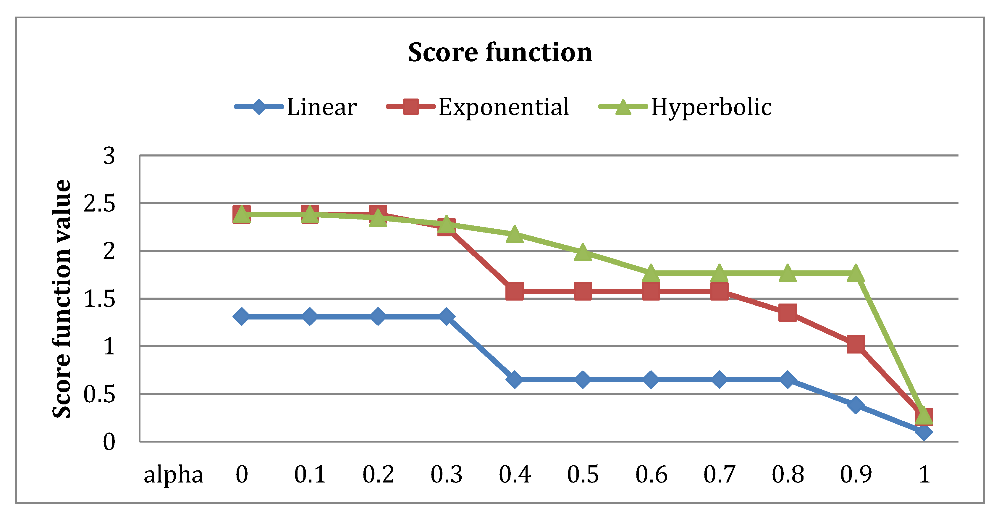
. In Table 3, the intuitionistic fuzzy membership values, intuitionistic fuzzy non-membership values corresponding to the given four fuzzy preference relations are tabulated along with the score function. The higher value of score function was better than smaller values, as it was the difference of membership and non-membership function values. From Table 3, it can be seen that for the case of linear preference relation, the sum of membership grades were decreasing for the values of $\alpha$. The non-membership grades were increasing, and as a result of them, the score function values were decreasing. For better visualisation of the score function, see, Figure 6. In case of linear FGP-IFPR, at $\alpha =0$, score function was 1.3091 whereas for $\alpha =1$, it became 0.098. For exponential and hyperbolic preference relation FGP-IFPR models, the same decreasing pattern was followed by the score function. On comparing the three FGP-IFPR models, the hyperbolic FGP-IFPR performed best for score function, and linear FGP-IFPR performed worst. At $\alpha =1$, the values were very much nearby for exponential and hyperbolic FGP-IFPR models.

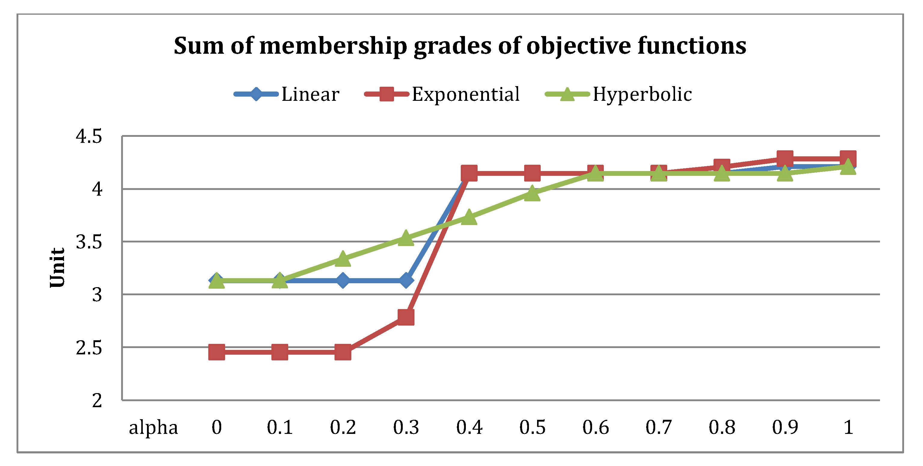
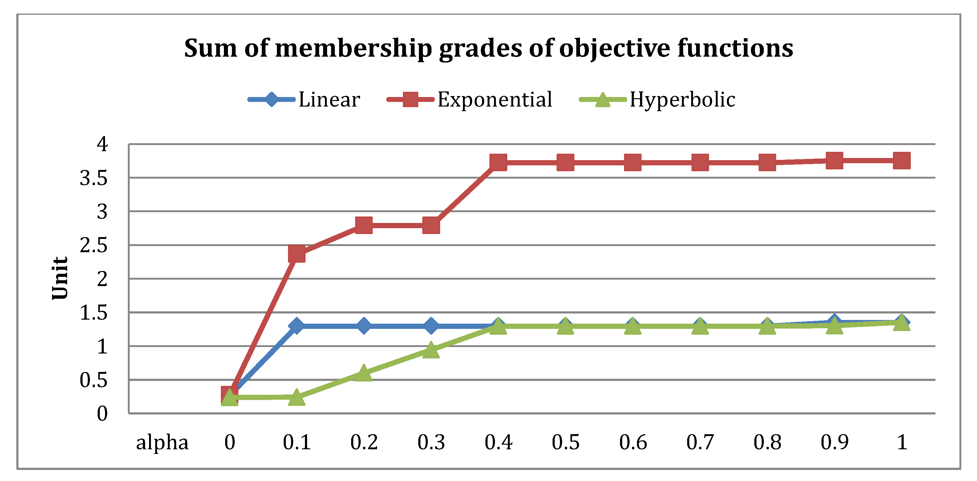
For the solution values of this example, the values of decision variables, optimal goal values and fuzzy goals and their individual membership grades were also evaluated. In Table 4, the solution values that are $x_1,x_2,x_3,\mathrm{and}{x}_4$, objective functions $Z_1,Z_2,Z_3,Z_4,\mathrm{and}{Z}_5$, and grades are presented. The values of sum of membership grades of objective functions, in case of linear, exponential and hyperbolic FGP-IFPR models continuously increases for values of $\alpha$. There was an increase in sum of membership grades for exponential FGP-IFPR model at $\alpha =0.4$, before that the values were less than linear FGP-IFPR model. In Figure 7, it is clear that from $\alpha =$ 0.4–1, exponential FGP-IFPR model have larger value of $\sum {\mu }_k$ than linear and hyperbolic FGP-IFPR models, whereas before 0.4 hyperbolic FGP-IFPR model gives better values for $\sum {\mu }_k$. There was much less difference for exponential and linear FGP-IFPR models from $\alpha =$ 0.4–0.7, whereas for hyperbolic and exponential FGP-IFPR models, the same values as from $\alpha =$ 0.6–0.7 applied.

5.3. Example 2: Banking Application

In this example, a real-life application was studied with the banking financial statement management system of Maybank. The data of financial statements are shown in

Table 5. Data summarized from Maybank financial statement from year 2010 to 2014 (RM’ trillion).

Goal			Year			Total	Aspiration Values
	2010	2011	2012	2013	2014
Asset	0.3367	0.4516	0.4948	0.5603	0.6403	2.4837	2.4941
Liability	0.3080	0.4157	0.4509	0.5126	0.5856	2.2729	2.2633
Equity	0.0287	0.0325	0.0438	0.0477	0.0547	0.2074	0.2207
Profit	0.0038	0.0026	0.0057	0.0066	0.0067	0.0254	0.0292
Earnings	0.2908	0.3766	0.4256	0.4792	0.5518	2.1241	2.1459
Total	0.9680	1.2790	1.4209	1.6064	1.8391	7.1135	7.1624

. They included total assets, liabilities, total equity, earning and profit, taken from Halim et al. [68]. We have given six objectives as Goal-1: assets, Goal-2: liabilities, Goal-3: equity, Goal-4: earning, Goal-5: profitability, and Goal-6: financial statement. The decision variables were:

$x_1$ = the amount of financial statement in year 2010.

$x_2$ = the amount of financial statement in year 2011.

$x_3$ = the amount of financial statement in year 2012.

$x_4$ = the amount of financial statement in year 2013.

$x_5$ = the amount of financial statement in year 2014.

The fuzzy goals were as follows:

$0.3367x_1+0.4516x_2+0.4948x_3+0.5603x_4+0.6403x_5\ge 2.4837$; (Goal 1)

$0.3080x_1+0.4157x_2+0.4509x_3+0.5126x_4+0.5856x_5\le 2.2729$; (Goal 2)

$0.0287x_1+0.0325x_2+0.0438x_3+0.0477x_4+0.0547x_5\ge 0.2074$; (Goal 3)

$0.0038x_1+0.0026x_2+0.0057x_3+0.0066x_4+0.0067x_5\ge 0.0254$; (Goal 4)

$0.2908x_1+0.3766x_2+0.4256x_3+0.4792x_4+0.5518x_5\ge 2.1241$; (Goal 5)

$0.9680x_1+1.2790x_2+1.4209x_3+1.6064x_4+1.8391x_5\ge 7.1135$; (Goal 6)

$x_1,x_2,x_3,x_4,x_5\ge 0$ (non-negativity restrictions)

Based on the discussion with experts, the type of linguistic preference relations among the bank financial statement goals were:

• Asset (Goal-1) is moderately more important than liability (Goal-2): ${\mu }_{12}$.
• Liability (Goal-2) is moderately more important than earning (Goal-4): ${\mu }_{24}$.
• Liability (Goal-2) is moderately more important than profitability (Goal-5): ${\mu }_{25}$.
• Asset (Goal-1) is moderately more important than profitability (Goal-5): ${\mu }_{15}$.

Now, the problem was solved using solution approach of Algorithm 1 by applying proposed FGP-IFPR models and results were obtained.

5.4. Solution Steps for Example 2

The solution steps are summarized as follows.

Step-1 Start with given multi-objective programming problem as follows:

$$\begin{array}{cc}\hfill \mathrm{Maximize}& Z_1=0.3367x_1+0.4516x_2+0.4948x_3+0.5603x_4+0.6403x_5\ge 2.4837\hfill \end{array}$$

(27a)

$$\begin{array}{cc}\hfill \mathrm{Minimize}& Z_2=0.3080x_1+0.4157x_2+0.4509x_3+0.5126x_4+0.5856x_5\le 2.2729\hfill \end{array}$$

(27b)

$$\begin{array}{cc}\hfill \mathrm{Maximize}& Z_3=0.0287x_1+0.0325x_2+0.0438x_3+0.0477x_4+0.0547x_5\ge 0.2074\hfill \end{array}$$

(27c)

$$\begin{array}{cc}\hfill \mathrm{Maximize}& Z_4=0.0038x_1+0.0026x_2+0.0057x_3+0.0066x_4+0.0067x_5\ge 0.0254\hfill \end{array}$$

(27d)

$$\begin{array}{cc}\hfill \mathrm{Maximize}& Z_5=0.2908x_1+0.3766x_2+0.4256x_3+0.4792x_4+0.5518x_5\ge 2.1241\hfill \end{array}$$

(27e)

$$\begin{array}{cc}\hfill \mathrm{Maximize}& Z_6=0.9680x_1+1.2790x_2+1.4209x_3+1.6064x_4+1.8391x_5\ge 7.1135\hfill \end{array}$$

(27f)

$$\begin{array}{cc}\hfill \mathrm{subject}\mathrm{to}& x_1,x_2,x_3,x_4,x_5\ge 0\hfill \end{array}$$

(27g)

Step-2 Formulate the problem as six single objective problems (based on the respective goals).

Step-3 On solving each optimization problem individually, we get the aspiration values, as given in Table 5. In addition, the upper limit for minimization fuzzy goal $Z_2$ is $u_2=2.2729$ and lower limits for maximization fuzzy goals $Z_1$ is $t_1=2.4837$, $Z_3$ is $t_3=0.2115$, $Z_4$ is $t_4=0.0280$, $Z_5$ is $t_5=2.1248$, $Z_6$ is $t_6=7.1228$, with $a_k$ as their corresponding aspiration levels.

Step-4 The membership function (${\mu }_k$) for each objective function $Z_k$ corresponding to each situation can be modeled using Equations (7) and (8) as follows:

$${\mu }_1=\frac{(Z_1-2.4837)}{(2.4941-2.4837)};{\mu }_2=\frac{(2.2729-Z_2)}{(2.2729-2.2633)};{\mu }_3=\frac{(Z_3-0.2115)}{(0.2207-0.2115)};$$

$${\mu }_4=\frac{(Z_4-0.0280)}{(0.0292-0.0280)};{\mu }_5=\frac{(Z_5-2.1248)}{(2.1459-2.1248)};{\mu }_6=\frac{(Z_6-7.122)}{(7.1624-7.1228)}.$$

Step-5 The intuitionistic fuzzy functions for the preference relations are presented in this step. Suppose ${\mu }_{12}$, ${\mu }_{24}$, ${\mu }_{25}$, and ${\mu }_{15}$ are the intuitionistic fuzzy membership function and ${\nu }_{12}$, ${\nu }_{24}$, ${\nu }_{25}$, and ${\nu }_{15}$ are intuitionistic fuzzy non-membership function with respect to the linguistic preference relations as given in problem definition. Thus, the linear membership function and non-membership function formulation for each preference relation using Equations (15a)–(15c) and Equations (16a)–(16c) are calculated as:

$${\mu }_{12}=\frac{({\mu }_1-{\mu }_2+1)}{2};{\mu }_{24}=\frac{({\mu }_2-{\mu }_4+1)}{2};{\mu }_{25}=\frac{({\mu }_2-{\mu }_5+1)}{2};{\mu }_{15}=\frac{({\mu }_1-{\mu }_5+1)}{2};$$

$$v_{12}=\frac{(1-{\mu }_1+{\mu }_2)}{2};v_{24}=\frac{(1-{\mu }_2+{\mu }_4)}{2};v_{25}=\frac{(1-{\mu }_2+{\mu }_5)}{2};v_{15}=\frac{(1-{\mu }_1+{\mu }_5)}{2};$$

The exponential membership function and non-membership function formulation for each preference relation using Equations (17a)–(17c) and Equations (18a)–(18c) are calculated as:

$${\mu }_{12}=\frac{(1-e^{-s.({\mu }_1-{\mu }_2+1)/2})}{(1-e^{-s})};{\mu }_{24}=\frac{(1-e^{-s.({\mu }_2-{\mu }_4+1)/2})}{(1-e^{-s})};$$

$${\mu }_{25}=\frac{(1-e^{-s.({\mu }_2-{\mu }_5+1)/2})}{(1-e^{-s})};{\mu }_{15}=\frac{(1-e^{-s.({\mu }_1-{\mu }_5+1)/2})}{(1-e^{-s})};$$

$$v_{12}=\frac{(e^{-s.({\mu }_1-{\mu }_2+1)/2}-e^{-s})}{(1-e^{-s})};v_{24}=\frac{(e^{-s.({\mu }_2-{\mu }_4+1)/2}-e^{-s})}{(1-e^{-s})};$$

$$v_{25}=\frac{(e^{-s.({\mu }_2-{\mu }_5+1)/2}-e^{-s})}{(1-e^{-s})};v_{15}=\frac{(e^{-s.({\mu }_1-{\mu }_5+1)/2}-e^{-s})}{(1-e^{-s})};$$

The hyperbolic membership function and non-membership function formulation for each preference relation using Equations (19a)–(19c) and Equations (20a)–(20c) are calculated as:

$${\mu }_{12}={\displaystyle \frac{e^{3({\mu }_1-{\mu }_2)}}{e^{-3({\mu }_1-{\mu }_2)}+e^{3({\mu }_1-{\mu }_2)}}};{\mu }_{24}={\displaystyle \frac{e^{3({\mu }_2-{\mu }_4)}}{e^{-3({\mu }_2-{\mu }_4)}+e^{3({\mu }_2-{\mu }_4)}}};$$

$${\mu }_{25}={\displaystyle \frac{e^{3({\mu }_2-{\mu }_5)}}{e^{-3({\mu }_2-{\mu }_5)}+e^{3({\mu }_2-{\mu }_5)}}};{\mu }_{15}={\displaystyle \frac{e^{3({\mu }_1-{\mu }_5)}}{e^{-3({\mu }_1-{\mu }_5)}+e^{3({\mu }_1-{\mu }_5)}}};$$

$$v_{12}={\displaystyle \frac{e^{-3({\mu }_1-{\mu }_2)}}{e^{-3({\mu }_1-{\mu }_2)}+e^{3({\mu }_1-{\mu }_2)}}};v_{24}={\displaystyle \frac{e^{-3({\mu }_2-{\mu }_4)}}{e^{-3({\mu }_2-{\mu }_4)}+e^{3({\mu }_2-{\mu }_4)}}};$$

$$v_{25}={\displaystyle \frac{e^{-3({\mu }_2-{\mu }_5)}}{e^{-3({\mu }_2-{\mu }_5)}+e^{3({\mu }_2-{\mu }_5)}}};v_{15}={\displaystyle \frac{e^{-3({\mu }_1-{\mu }_5)}}{e^{-3({\mu }_1-{\mu }_5)}+e^{3({\mu }_1-{\mu }_5)}}};$$

Step-6 Problem formulations: The FGP-IFPR model of numerical Example-2 are formulated using preference relation functions. We have applied three different kinds of intuitionistic fuzzy functions for preference relations, namely, linear, exponential, and hyperbolic, there will be three different formulations.

Formulation I: FGP-IFPR for linear.

$$\begin{array}{cc}\hfill \mathrm{Maximize}& \alpha .({\mu }_1+{\mu }_2+{\mu }_3+{\mu }_4+{\mu }_5+{\mu }_6)+(1-\alpha ).(S_{12}+S_{24}+S_{25}+S_{32})\hfill \\ \hfill \mathrm{subject}\mathrm{to},& \hfill \end{array}$$

(28a)

$$\begin{array}{cc}\hfill & {\mu }_{12}\le \frac{({\mu }_1-{\mu }_2+1)}{2};{\mu }_{24}\le \frac{({\mu }_2-{\mu }_4+1)}{2};{\mu }_{25}\le \frac{({\mu }_2-{\mu }_5+1)}{2};{\mu }_{15}\le \frac{({\mu }_1-{\mu }_5+1)}{2}\hfill \end{array}$$

(28b)

$$\begin{array}{cc}\hfill & v_{12}\ge \frac{(1-{\mu }_1+{\mu }_2)}{2};v_{24}\ge \frac{(1-{\mu }_2+{\mu }_4)}{2};v_{25}\ge \frac{(1-{\mu }_2+{\mu }_5)}{2};v_{15}\ge \frac{(1-{\mu }_1+{\mu }_5)}{2}\hfill \end{array}$$

(28c)

$$\begin{array}{cc}\hfill & {\mu }_1=\frac{(Z_1-2.4837)}{(2.4941-2.4837)};{\mu }_2=\frac{(2.2729-Z_2)}{(2.2729-2.2633)};{\mu }_3=\frac{(Z_3-0.2115)}{(0.2207-0.2115)};\hfill \end{array}$$

(28d)

$$\begin{array}{cc}\hfill & {\mu }_4=\frac{(Z_4-0.0280)}{(0.0292-0.0280)};{\mu }_5=\frac{(Z_5-2.1248)}{(2.1459-2.1248)};{\mu }_6=\frac{(Z_6-7.122)}{(7.1624-7.1228)}\hfill \end{array}$$

(28e)

$$\begin{array}{cc}\hfill & S_{12}={\mu }_{12}-v_{12};S_{24}={\mu }_{24}-v_{24};S_{25}={\mu }_{25}-v_{25};S_{32}={\mu }_{15}-v_{15};\hfill \end{array}$$

(28f)

$$\begin{array}{cc}\hfill & 1\ge {\mu }_{12}\ge v_{12}\ge 0;1\ge {\mu }_{24}\ge v_{24}\ge 0;1\ge {\mu }_{25}\ge v_{25}\ge 0;1\ge {\mu }_{15}\ge v_{15}\ge 0;\hfill \end{array}$$

(28g)

$$\begin{array}{cc}\hfill & 0\le {\mu }_{12}+v_{12}\le 1;0\le {\mu }_{24}+v_{24}\le 1;0\le {\mu }_{25}+v_{25}\le 1;0\le {\mu }_{15}+v_{15}\le 1;\hfill \end{array}$$

(28h)

$$\begin{array}{cc}\hfill & 0\le {\mu }_1\le 1;0\le {\mu }_2\le 1;0\le {\mu }_3\le 1;0\le {\mu }_4\le 1;0\le {\mu }_5\le 1;0\le {\mu }_6\le 1.\hfill \end{array}$$

(28i)

Formulation II: FGP-IFPR for exponential.

$$\begin{array}{cc}\hfill \mathrm{Maximize}& \alpha .({\mu }_1+{\mu }_2+{\mu }_3+{\mu }_4+{\mu }_5+{\mu }_6)+(1-\alpha ).(S_{12}+S_{24}+S_{25}+S_{32})\hfill \\ \hfill \mathrm{subject}\mathrm{to},& \hfill \end{array}$$

(29a)

$$\begin{array}{cc}\hfill & {\mu }_{12}\le \frac{(1-e^{-s.({\mu }_1-{\mu }_2+1)/2})}{(1-e^{-s})};{\mu }_{24}\le \frac{(1-e^{-s.({\mu }_2-{\mu }_4+1)/2})}{(1-e^{-s})};\hfill \end{array}$$

(29b)

$$\begin{array}{cc}\hfill & {\mu }_{25}\le \frac{(1-e^{-s.({\mu }_2-{\mu }_5+1)/2})}{(1-e^{-s})};{\mu }_{15}\le \frac{(1-e^{-s.({\mu }_1-{\mu }_5+1)/2})}{(1-e^{-s})}\hfill \end{array}$$

(29c)

$$\begin{array}{cc}\hfill & v_{12}\ge \frac{(e^{-s.({\mu }_1-{\mu }_2+1)/2}-e^{-s})}{(1-e^{-s})};v_{24}\ge \frac{(e^{-s.({\mu }_2-{\mu }_4+1)/2}-e^{-s})}{(1-e^{-s})}\hfill \end{array}$$

(29d)

$$\begin{array}{cc}\hfill & v_{25}\ge \frac{(e^{-s.({\mu }_2-{\mu }_5+1)/2}-e^{(-s)})}{(1-e^{-s})};v_{15}\ge \frac{(e^{-s.({\mu }_1-{\mu }_5+1)/2}-e^{-s})}{(1-e^{-s})}\hfill \end{array}$$

(29e)

Equations (28f)–(28i)

Formulation III: FGP-IFPR for hyperbolic.

$$\begin{array}{cc}\hfill \mathrm{Maximize}& \alpha .({\mu }_1+{\mu }_2+{\mu }_3+{\mu }_4+{\mu }_5+{\mu }_6)+(1-\alpha ).(S_{12}+S_{24}+S_{25}+S_{32})\hfill \\ \hfill \mathrm{subject}\mathrm{to},& \hfill \end{array}$$

(30a)

$$\begin{array}{cc}\hfill & {\mu }_{12}\le {\displaystyle \frac{e^{3({\mu }_1-{\mu }_2)}}{e^{-3({\mu }_1-{\mu }_2)}+e^{3({\mu }_1-{\mu }_2)}}};{\mu }_{24}\le {\displaystyle \frac{e^{3({\mu }_2-{\mu }_4)}}{e^{-3({\mu }_2-{\mu }_4)}+e^{3({\mu }_2-{\mu }_4)}}};\hfill \end{array}$$

(30b)

$$\begin{array}{cc}\hfill & {\mu }_{25}\le {\displaystyle \frac{e^{3({\mu }_2-{\mu }_5)}}{e^{-3({\mu }_2-{\mu }_5)}+e^{3({\mu }_2-{\mu }_5)}}};{\mu }_{15}\le {\displaystyle \frac{e^{3({\mu }_1-{\mu }_5)}}{e^{-3({\mu }_1-{\mu }_5)}+e^{3({\mu }_1-{\mu }_5)}}}\hfill \end{array}$$

(30c)

$$\begin{array}{cc}\hfill & v_{12}\ge {\displaystyle \frac{e^{-3({\mu }_1-{\mu }_2)}}{e^{-3({\mu }_1-{\mu }_2)}+e^{3({\mu }_1-{\mu }_2)}}};v_{24}\ge {\displaystyle \frac{e^{-3({\mu }_2-{\mu }_4)}}{e^{-3({\mu }_2-{\mu }_4)}+e^{3({\mu }_2-{\mu }_4)}}};\hfill \end{array}$$

(30d)

$$\begin{array}{cc}\hfill & v_{25}\ge {\displaystyle \frac{e^{-3({\mu }_2-{\mu }_5)}}{e^{-3({\mu }_2-{\mu }_5)}+e^{3({\mu }_2-{\mu }_5)}}};v_{15}\ge {\displaystyle \frac{e^{-3({\mu }_1-{\mu }_5)}}{e^{-3({\mu }_1-{\mu }_5)}+e^{3({\mu }_1-{\mu }_5)}}};\hfill \end{array}$$

(30e)

Equations (28f)–(28i)

Step-7 Now, we solve the above FGP-IFPR model of Example 2 using any linear and non linear optimization solver and software.

Step-8 Stop, the optimal and feasible solution is obtained.

Results and Discussion for Example 2

The problem solved in Example 2 was a real-life problem. The solutions i.e., amount of financial statement in 2010, 2011, 2012, 2013, and 2014 ($x_1,x_2,x_3,x_4,\mathrm{and}{x}_5$) were determined. The problem consisted of six different goals. Similar to Example 1, membership grade, non-membership grades, goal values and their satisfaction levels were determined and presented in

Table 6. Result values for preference membership, non-membership grades and score function of fuzzy goal programming with intuitionistic fuzzy relations (FGP-IFPR) for Example 2.

Formulation	$\mathit{\alpha }$	${\mathit{\mu }}_{12}$	${\mathit{\mu }}_{24}$	${\mathit{\mu }}_{25}$	${\mathit{\mu }}_{15}$	$\sum {\mathit{\mu }}_{{\mathit{R}}_{\mathit{i}}}(\mathit{k},\mathit{l})$	${\mathit{v}}_{12}$	${\mathit{\nu }}_{24}$	${\mathit{\nu }}_{25}$	${\mathit{\nu }}_{15}$	$\sum {\mathit{\nu }}_{{\mathit{R}}_{\mathit{i}}}(\mathit{k},\mathit{l})$	$\sum {\mathit{S}}_{{\mathit{R}}_{\mathit{i}}}(\mathit{k},\mathit{l})$
I:FGP-IFPR	0.0	0.5834	0.5120	0.5834	0.5000	2.1789	0.4165	0.4879	0.4165	0.5000	1.8209	0.3579
for Linear	0.1	0.5000	0.6286	0.5000	0.5000	2.1286	0.5000	0.3713	0.5000	0.5000	1.8713	0.2572
	0.2	0.5000	0.6286	0.5000	0.5000	2.1286	0.5000	0.3713	0.5000	0.5000	1.8713	0.2572
	0.3	0.5000	0.6286	0.5000	0.5000	2.1286	0.5000	0.3713	0.5000	0.5000	1.8713	0.2572
	0.4	0.5000	0.6286	0.5000	0.5000	2.1286	0.5000	0.3713	0.5000	0.5000	1.8713	0.2572
	0.5	0.5000	0.6286	0.5000	0.5000	2.1286	0.5000	0.3713	0.5000	0.5000	1.8713	0.2572
	0.6	0.5000	0.6286	0.5000	0.5000	2.1286	0.5000	0.3713	0.5000	0.5000	1.8713	0.2572
	0.7	0.5000	0.6286	0.5000	0.5000	2.1286	0.5000	0.3713	0.5000	0.5000	1.8713	0.2572
	0.8	0.5000	0.6286	0.5000	0.5000	2.1286	0.5000	0.3713	0.5000	0.5000	1.8713	0.2572
	0.9	0.5000	0.5000	0.5000	0.5000	2.0000	0.5000	0.5000	0.5000	0.5000	2.0000	0.0000
	1.0	0.5000	0.5000	0.5000	0.5000	2.0000	0.5000	0.5000	0.5000	0.5000	2.0000	0.0000
II:FGP-IFPR	0.0	0.7029	0.6320	0.6198	0.7004	2.6500	0.2971	0.3680	0.3802	0.2996	1.3450	1.3100
for Exponential	0.1	0.7145	0.7489	0.5000	0.6038	2.5672	0.2855	0.2511	0.5000	0.3962	1.4328	1.1344
	0.2	0.6842	0.7879	0.5000	0.5696	2.5417	0.3158	0.2121	0.5000	0.4304	1.4583	1.0835
	0.3	0.6842	0.7879	0.5000	0.5696	2.5417	0.3158	0.2121	0.5000	0.4304	1.4583	1.0835
	0.4	0.6225	0.6337	0.5000	0.5000	2.2562	0.3775	0.3663	0.5000	0.5000	1.7438	0.5124
	0.5	0.6225	0.6337	0.5000	0.5000	2.2562	0.3775	0.3663	0.5000	0.5000	1.7438	0.5124
	0.6	0.6225	0.6337	0.5000	0.5000	2.2562	0.3775	0.3663	0.5000	0.5000	1.7438	0.5124
	0.7	0.6225	0.6337	0.5000	0.5000	2.2562	0.3775	0.3663	0.5000	0.5000	1.7438	0.5124
	0.8	0.6225	0.6337	0.5000	0.5000	2.2562	0.3775	0.3663	0.5000	0.5000	1.7438	0.5124
	0.9	0.6225	0.5654	0.5000	0.5000	2.1879	0.3775	0.4346	0.5000	0.5000	1.8121	0.3758
	1.0	0.4827	0.4869	0.5000	0.5000	1.9696	0.4221	0.4528	0.5000	0.5000	1.8750	0.0946
III:FGP-IFPR	0.0	0.6438	0.5880	0.5701	0.7057	2.5077	0.3562	0.4120	0.4299	0.2943	1.4924	1.0151
for Hyperbolic	0.1	0.6538	0.5825	0.5627	0.7085	2.5075	0.3462	0.4175	0.4373	0.2915	1.4926	1.0149
	0.2	0.6634	0.6446	0.5000	0.6634	2.4715	0.3366	0.3554	0.5000	0.3366	1.5285	0.9430
	0.3	0.5849	0.7435	0.5000	0.5849	2.4134	0.4151	0.2565	0.5000	0.4151	1.5867	0.8267
	0.4	0.5000	0.8240	0.5000	0.5000	2.3240	0.5000	0.1760	0.5000	0.5000	1.6760	0.6479
	0.5	0.5000	0.8240	0.5000	0.5000	2.3240	0.5000	0.1760	0.5000	0.5000	1.6760	0.6479
	0.6	0.5000	0.8240	0.5000	0.5000	2.3240	0.5000	0.1760	0.5000	0.5000	1.6760	0.6479
	0.7	0.5000	0.8240	0.5000	0.5000	2.3240	0.5000	0.1760	0.5000	0.5000	1.6760	0.6480
	0.8	0.5000	0.8240	0.5000	0.5000	2.3240	0.5000	0.1760	0.5000	0.5000	1.6760	0.6480
	0.9	0.5000	0.7967	0.5000	0.5000	2.2967	0.5000	0.2033	0.5000	0.5000	1.7033	0.5934
	1.0	0.5000	0.5000	0.5000	0.5000	2.0000	0.5000	0.5000	0.5000	0.5000	2.0000	0.0000

and

Table 7. Result values for solution: Objective functions and their membership grade of FGP-IFPR for Example 2.

Formulation	$\mathit{\alpha }$	${\mathit{x}}_1$	${\mathit{x}}_2$	${\mathit{x}}_3$	${\mathit{x}}_4$	${\mathit{x}}_5$	${\mathit{Z}}_1$	${\mathit{Z}}_2$	${\mathit{Z}}_3$	${\mathit{Z}}_4$	${\mathit{Z}}_5$	${\mathit{Z}}_6$	${\mathit{\mu }}_1$	${\mathit{\mu }}_2$	${\mathit{\mu }}_3$	${\mathit{\mu }}_4$	${\mathit{\mu }}_5$	${\mathit{\mu }}_6$	$\sum {\mathit{\mu }}_{\mathit{k}}$
I:FGP-IFPR	0.0	0.000	0.4058	1.3717	2.8978	0.0000	2.4856	2.2726	0.2115	0.0280	2.1253	7.1233	0.1909	0.0240	0.0000	0.0000	0.02400	0.0328	0.2718
for Linear	0.1	0.0000	0.3371	2.8886	1.6148	0.0000	2.4863	2.2704	0.2145	0.0280	2.1302	7.1298	0.2572	0.2572	0.3271	0.0000	0.2572	0.1977	1.2966
	0.2	0.0000	0.3371	2.8886	1.6148	0.0000	2.4863	2.2704	0.2145	0.0280	2.1300	7.1298	0.2572	0.2572	0.3271	0.0000	0.2572	0.1977	1.2966
	0.3	0.0000	0.3371	2.8886	1.6148	0.0000	2.4863	2.2704	0.2145	0.0280	2.1302	7.1298	0.2572	0.2572	0.3271	0.0000	0.2572	0.1977	1.2966
	0.4	0.0000	0.3371	2.8886	1.6148	0.0000	2.4863	2.2704	0.2145	0.0280	2.1302	7.1298	0.2572	0.2572	0.3271	0.0000	0.2572	0.1977	1.2966
	0.5	0.0000	0.3371	2.8886	1.6148	0.0000	2.4863	2.2704	0.2145	0.0280	2.1302	7.1298	0.2572	0.2572	0.3271	0.0000	0.2572	0.1977	1.2966
	0.6	0.0000	0.3371	2.8886	1.6148	0.0000	2.4863	2.2703	0.2145	0.0280	2.1302	7.1298	0.2572	0.2572	0.3271	0.0000	0.2572	0.1977	1.2966
	0.7	0.0000	0.3371	2.8886	1.6148	0.0000	2.4863	2.2704	0.2145	0.0280	2.1302	7.1298	0.2572	0.2572	0.3271	0.0000	0.2572	0.1977	1.2966
	0.8	0.0000	0.3371	2.8886	1.6148	0.0000	2.4863	2.2704	0.2145	0.0280	2.1302	7.1298	0.2572	0.2572	0.3271	0.0000	0.2572	0.1977	1.2966
	0.9	0.0000	0.2600	2.4077	2.1010	0.0000	2.4860	2.2707	0.2141	0.0282	2.1295	7.1289	0.2228	0.2228	0.2860	0.2228	0.2228	0.1747	1.3521
	1.0	0.0000	0.2600	2.4077	2.1010	0.0000	2.4860	2.2707	0.2141	0.0282	2.1295	7.1289	0.2228	0.2228	0.2860	0.2228	0.2228	0.1747	1.3521
II:FGP-IFPR	0.0	0.0000	0.4061	1.3705	2.8989	0.0000	2.4857	2.2727	0.2115	0.0280	2.1253	7.1234	0.1949	0.0199	0.0000	0.0000	0.0254	0.0356	0.2758
for Exponential	0.1	0.0000	0.2869	4.1703	0.5278	0.0000	2.4887	2.2702	0.2176	0.0280	2.1358	7.1403	0.4843	0.2827	0.6150	0.0000	0.5229	0.4629	2.3678
	0.2	0.0000	0.2586	4.7943	0.0000	0.0000	2.4890	2.2693	0.2184	0.0280	2.1379	7.1430	0.5116	0.3786	0.7496	0.000	0.6188	0.5308	2.7894
	0.3	0.0000	0.2586	4.7943	0.0000	0.0000	2.4890	2.2693	0.2184	0.0280	2.1379	7.1430	0.5116	0.3786	0.7496	0.0000	0.6188	0.5308	2.7894
	0.4	0.0000	0.0417	4.9917	0.0000	0.0000	2.4888	2.2682	0.2200	0.0286	2.1403	7.1463	0.4920	0.4920	0.9239	0.4684	0.7323	0.6138	3.7224
	0.5	0.0000	0.0417	4.9917	0.0000	0.0000	2.4888	2.2682	0.2200	0.0286	2.1403	7.1463	0.4920	0.4920	0.9239	0.4684	0.7323	0.6138	3.7224
	0.6	0.0000	0.0417	4.9917	0.0000	0.0000	2.4888	2.2682	0.2200	0.0286	2.1403	7.1463	0.4920	0.4920	0.9239	0.4684	0.7323	0.6138	3.7224
	0.7	0.0000	0.0417	4.9917	0.0000	0.0000	2.4888	2.2682	0.2200	0.0286	2.1403	7.1463	0.4920	0.4920	0.9239	0.4684	0.7323	0.6138	3.7224
	0.8	0.0000	0.0417	4.9917	0.0000	0.0000	2.4888	2.2682	0.2200	0.0286	2.1403	7.1463	0.4920	0.4920	0.9239	0.4684	0.7323	0.6138	3.7224
	0.9	0.0000	0.0000	4.7318	0.2629	0.0000	2.4886	2.2684	0.2198	0.0287	2.1399	7.1458	0.4734	0.4734	0.9017	0.5889	0.7137	0.6013	3.7525
	1.0	0.0000	0.0000	4.7318	0.2629	0.0000	2.4886	2.2684	0.2198	0.0287	2.1399	7.1458	0.4734	0.4734	0.9017	0.5889	0.7137	0.6013	3.7525
III:FGP-IFPR	0.0	0.0000	0.4039	1.3822	2.8897	0.0000	2.4853	2.2723	0.2115	0.0280	2.1251	7.1224	0.1579	0.0594	0.0000	0.0000	0.0122	0.0093	0.2387
for Hyperbolic	0.1	0.0000	0.4041	1.3810	2.8905	0.0000	2.4854	2.2724	0.2115	0.0280	2.1251	7.1225	0.1615	0.0555	0.0000	0.0000	0.0135	0.0118	0.2423
	0.2	0.0000	0.3837	1.8610	2.4841	0.0000	2.4859	2.2720	0.2125	0.0280	2.1269	7.1254	0.2124	0.0992	0.1055	0.0000	0.0993	0.0860	0.6024
	0.3	0.0000	0.3607	2.3693	2.0541	0.0000	2.4861	2.2712	0.2135	0.0280	2.1285	7.1276	0.2346	0.1774	0.2151	0.0000	0.1774	0.1413	0.9458
	0.4	0.0000	0.3372	2.8886	1.6149	0.0000	2.4864	2.2704	0.2145	0.0280	2.1302	7.1298	0.2572	0.2572	0.3271	0.0000	0.2572	0.1978	1.2967
	0.5	0.0000	0.3372	2.8886	1.6149	0.0000	2.4864	2.2704	0.2145	0.0280	2.1302	7.1298	0.2572	0.2572	0.3271	0.0000	0.2572	0.1978	1.2966
	0.6	0.0000	0.3372	2.8886	1.6149	0.0000	2.4864	2.2704	0.2145	0.0280	2.1302	7.1298	0.2572	0.2572	0.3271	0.0000	0.2572	0.1978	1.2966
	0.7	0.0000	0.3372	2.8886	1.6149	0.0000	2.4864	2.2704	0.2145	0.0280	2.1302	7.1298	0.2572	0.2572	0.3271	0.0000	0.2572	0.1978	1.2966
	0.8	0.0000	0.3372	2.8886	1.6149	0.0000	2.4864	2.2704	0.2145	0.0280	2.1302	7.1298	0.2572	0.2572	0.3271	0.0000	0.2572	0.1978	1.2966
	0.9	0.0000	0.3283	2.8332	1.6709	0.0000	2.4863	2.2705	0.2145	0.0280	2.1301	7.1297	0.2533	0.2533	0.3224	0.0257	0.2533	0.1951	1.3030
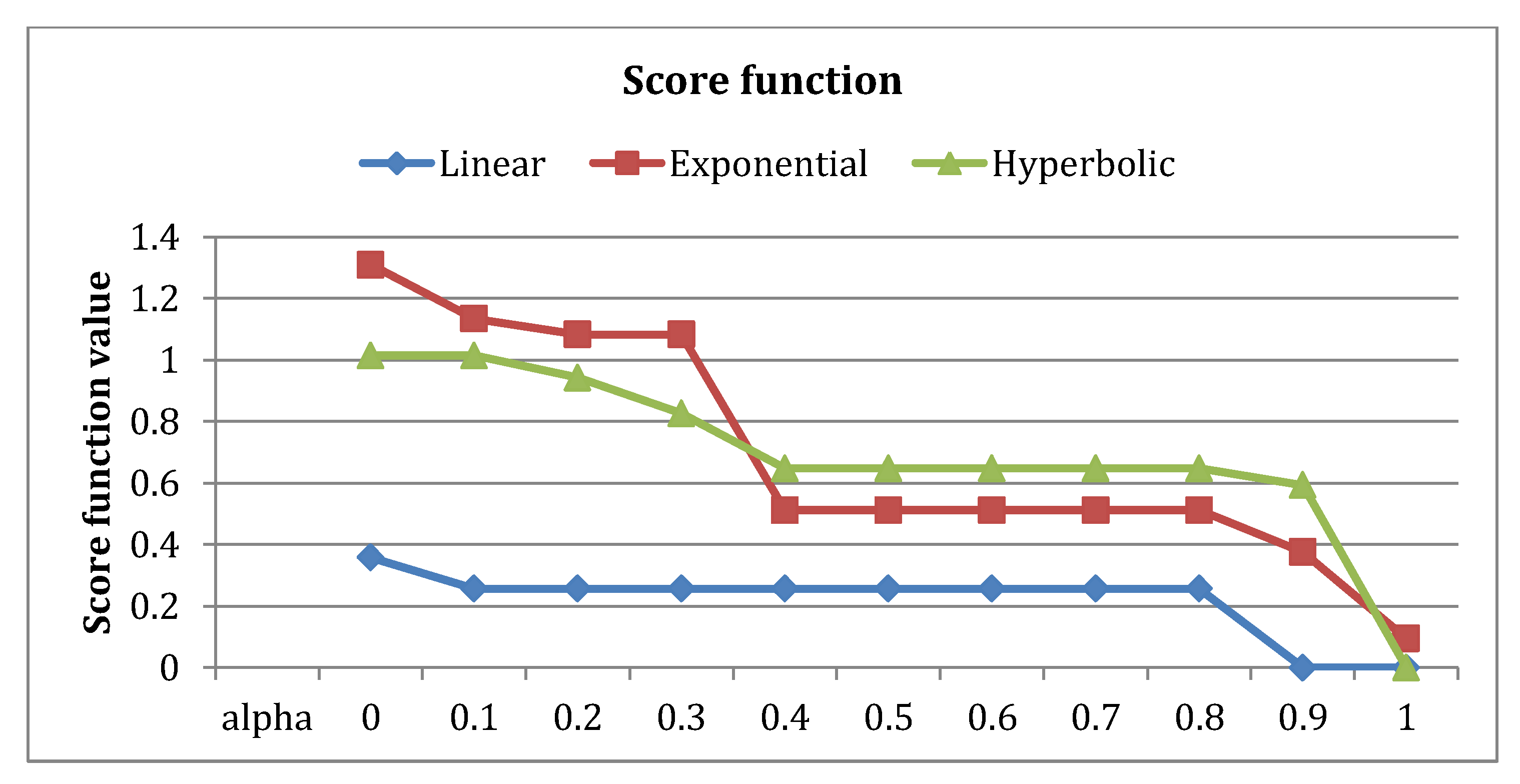
	1.0	0.0000	0.2600	2.4078	2.1011	0.0000	2.4860	2.2708	0.2141	0.0283	2.1295	7.1289	0.2228	0.2228	0.2861	0.2228	0.2228	0.1748	1.3522

. In Table 6, the preference membership grades decreased for linear and exponential FGP-IFPR models from $\alpha =$ 0.0–1.0 whereas it increased for non-membership grades. As a result, score function decreased for increasing values of $\alpha$. For hyperbolic FGP-IFPR model, it was similar to linear and exponential FGP-IFPR models from $\alpha =$ 0–0.9. At $\alpha =1$, there was an increase in score function value from 0 to 0.5933.

The value of score function remained constant for multiple values of $\alpha$. For linear FGP-IFPR, it remained constant as 0.2572 for $\alpha =$ 0.2–0.8 and became 0 for $\alpha =$ 0.9–1. For exponential FGP-IFPR model, the score function was 1.08345 for $\alpha =$ 0.2–0.3, then again it became constant with value 0.5124 for $\alpha =$ 0.4–0.8. If we see Figure 8, the hyperbolic FGP-IFPR model from $\alpha =$ 0.4–0.9 performed better for score function values than other models, whereas linear FGP-IFPR model performed worst among all FGP-IFPR models from $\alpha =$ 0–1. In Table 7 and Figure 9, the sum of individual membership grades $\sum {\mu }_k$ also tended towards increased value for all models of linear, exponential and hyperbolic preference relations. If we compared all three models, the exponential FGP-IFPR had the larger value of $\sum {\mu }_k$ for all values of $\alpha$. The solution values of all the objectives are also provided in Table 7.

5.5. Efficiency Analysis

The proposed method was applied to solve two experimental problems. Example 1 was a numerical problem and Example 2 was a banking financial statement problem. The procedure followed the solution algorithm explained in Section 4 beginning with determining the individual best and worst objective function values, then the choice and construction of membership and non-membership functions based on decision maker linguistic preference relation and constructing FGP-IFPR. The computational time was acceptable for all the problem models.

Here, FGP-IFPR models for linear, exponential and hyperbolic membership functions provided different optimal solutions. To determine the efficiency of the FGP-IFPR approach, we evaluated the degree of closeness of the outcome to the optimal solution for the different models. To measure closeness, the distance function was utilized, see Pramanik and Roy [69], Zheng et al. [70] and Zhao et al. [51]. A new distance function for selecting the priority solution for the proposed FGP-IFPR models was introduced in this paper.

$$D\left(x\right)={\left(\sum _{k=1}^K{(1-{\mu }_k)}^2+\sum _{k=1}^K{(1-S_{R_i}(k,l))}^2\right)}^{1/2}$$

(31)

The distance function with smaller value provided the most satisfying solution as it represented the best solution among all other solutions. Furthermore, the proposed FGP-IFPR approach considered a utility function divided into two criteria, namely: (1) sum of individual membership function and (2) sum of preference membership function achievement level. Based on these two criteria with a different value of $\alpha$, the performance of the different FGP-IFPR models could be analyzed. In

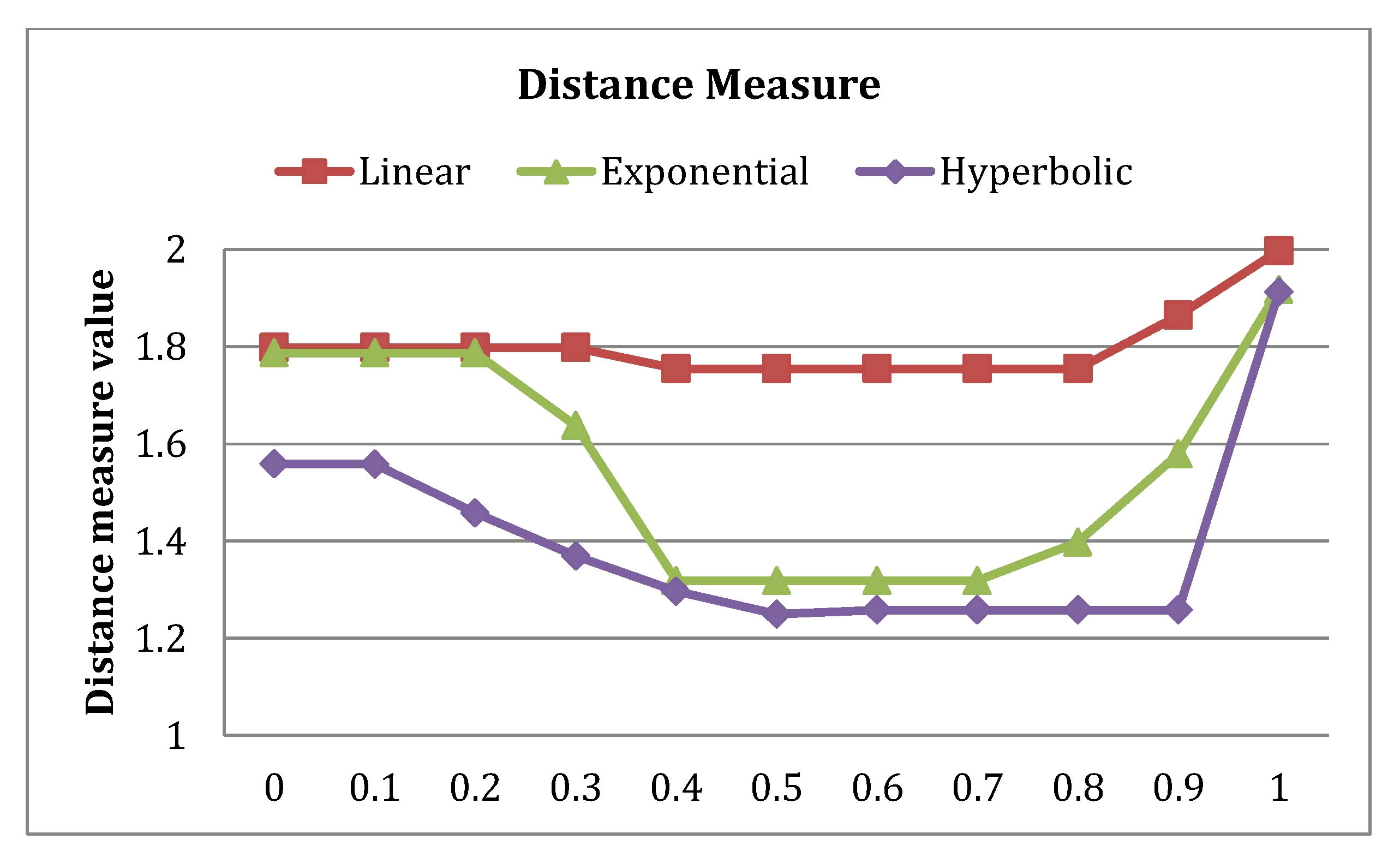
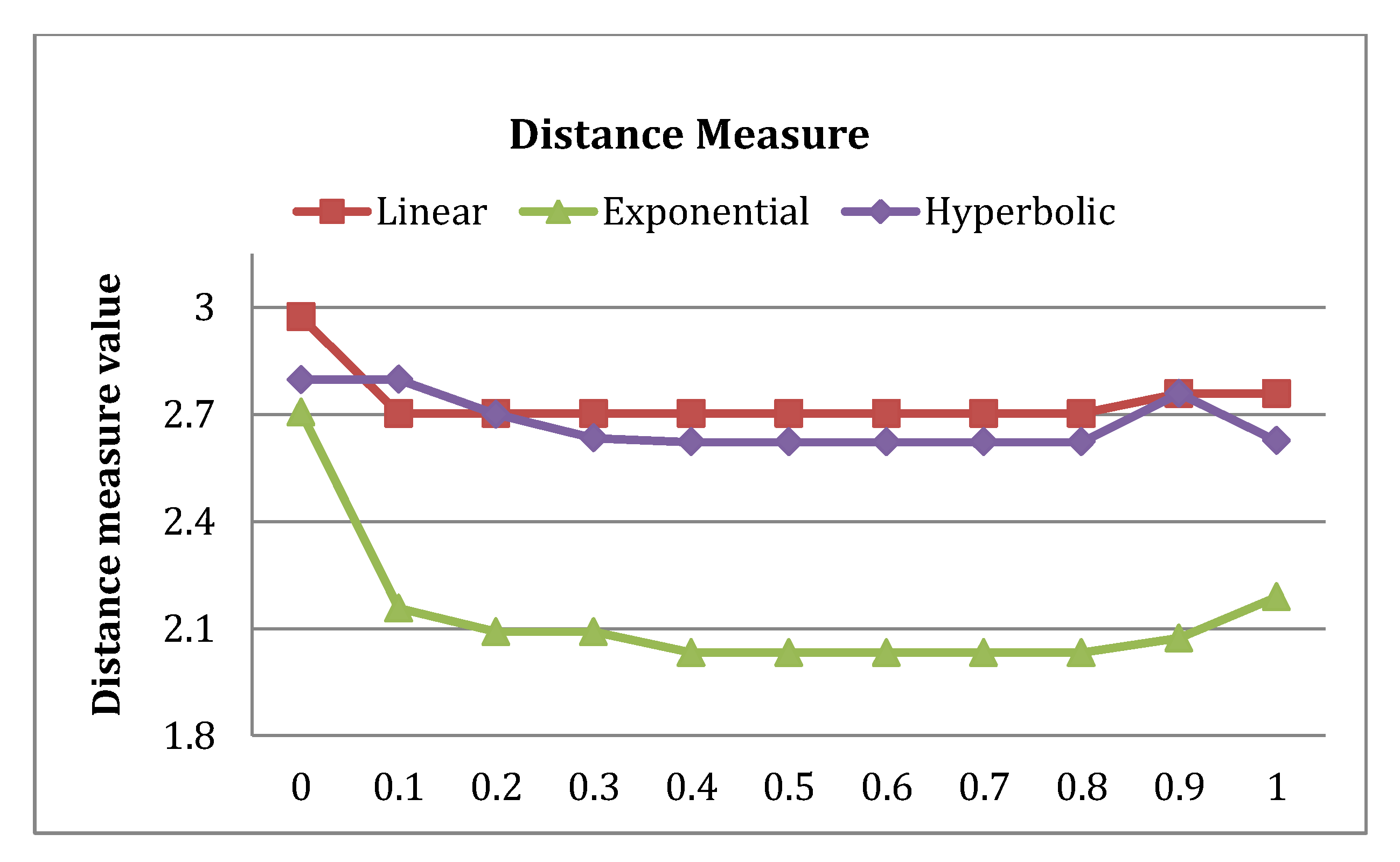
Table 8. Distance function values.

	FGP-IFPR for Example 1			FGP-IFPR for Example 2
$\mathbf{\alpha }$	Linear	Exponential	Hyperbolic	Linear	Exponential	Hyperbolic
0.0	1.7975	1.7864	1.5588	2.9724	2.7057	2.7971
0.1	1.7975	1.7864	1.5579	2.7024	2.1566	2.7976
0.2	1.7975	1.7864	1.4573	2.7024	2.0911	2.7000
0.3	1.7975	1.6376	1.3693	2.7024	2.0911	2.6333
0.4	1.7543	1.3184	1.2967	2.7024	2.0328	2.6221
0.5	1.7543	1.3184	1.2496	2.7024	2.0328	2.6221
0.6	1.7543	1.3184	1.2584	2.7024	2.0328	2.6221
0.7	1.7543	1.3184	1.2584	2.7024	2.0328	2.6221
0.8	1.7543	1.3980	1.2585	2.7024	2.0328	2.6221
0.9	1.8640	1.5789	1.2584	2.7580	2.0736	2.7580
1.0	1.9969	1.9171	1.9125	2.7580	2.1885	2.6257

, Figure 10 and Figure 11, the results for distance function values are tabulated and plotted for different values of $\alpha$ and for three of FGP-IFPR models. In Figure 10, for Example 1, at all values of $\alpha =0-1$, the hyperbolic FGP-IFPR model performed best, and linear FGP-IFPR performed worst. The overall performance ranking was $Hyperbolic>Exponential>Linear$. For Example 2, at $\alpha =0.1$, the performance pattern was $Exponential>Linear>Hyperbolic$, whereas for rest of the values of $\alpha$, it is $Exponential>Hyperbolic>Linear$ see in Figure 11. It can be seen that, with respect the problem type and value of $\alpha$, the performance of linear, exponential and hyperbolic FGP-IFPR models changed.

6. Conclusions, Limitations, and Future Directions

The paper aims to propose a fuzzy goal programming with intuitionistic fuzzy preference relations (FGP-IFPR) approach. The FGP-IFPR model involves the achievement of the fuzzy goals and uncertain preference relationships among goals with the degree of belongingness and non-belongingness, simultaneously. Linguistically imprecise relation represents the associations amongst the fuzzy goals. The IFPRs among goals are addressed as linear and non-linear (exponential and hyperbolic) functions. The use of non-linear functions for the imprecise relative importance among fuzzy objective lead towards the more realistic representation of the linguistic term and provide flexibility in the decision-making process. The perception of intuitionistic fuzzy exponential and hyperbolic functions have more justified significance because it can smoothly overcome the weaknesses associated with the structure of the Gaussian function amidst non-zero functional values affecting its broad range of the footprint. The mathematical expressibility of intuitionistic fuzzy exponential and hyperbolic functions only requires two parametric values. The objective function of FGP-IFPR is a convex combination of membership degrees of fuzzy goals and score function of the IFPRs. We presented the three linear, exponential, and hyperbolic FGP-IFPR formulations and an extensive step by step solutions procedure to find the optimal solutions for these formulated models. An experimental study is done to provide a comprehensive validation of these approaches. Two numerical examples are considered for proposed models. The first example is a numerical problem, and the second example is the banking financial statement problem. For both instances, the optimal goal values, decision variables, and fuzzy goals are evaluated along with the grades and total score values to three FGP-IFPR models for different values of the weighted objective parameter. On the analysis of the obtained optimal solutions to three FGP-IFPR models by using the distance function, it has been found that, in case of example 1, the FGP-IFPR for hyperbolic performs best and FGP-IFPR for linear performs worst. The ranking of the efficiency of FGP-IFPR models is $Hyperbolic>Exponential>Linear$. For example 2, the ranking of the efficiency of FGP-IFPR models is $Exponential>Hyperbolic>Linear$.

The proposed FGP-IFPR framework has multiple advantages over several existing approaches in terms of: (1) better representation of uncertain importance relations among goals, (2) including the concept of the intuitionistic fuzzy set for preference relations, (3) simultaneously evaluating the degree of belongingness and non-belongingness, (4) preventing the difficulty of providing weights to the goals, and (5) enhancing the membership degree as well as efficiently reduce the non-membership degree. All the existing methods dealt only with the linear fuzzy preference relations. The limitation of the work is that the judgements are drawn based on considered models that may change according to the problem. Further, only three types of preference relations namely “slightly more important”, or “moderately more important”, or “significantly more important” are considered.

In the future, we will increase the numbers of preference relations, that are needed to represent by the intuitionistic fuzzy exponential and hyperbolic functions. The proposed models can be applied to a large number of real-life applications where the number of objectives is enormous, for example, manufacturing, human resource management, sustainable economy, forest management, portfolio optimization. This work can be further extended to the FGP-IFPR model with other non-linear functions like parabolic, s-curve, and so on, and its applications to real-life problems.