Effective Boundary of Innovation Subsidy: Searching by Stochastic Evolutionary Game Model

Abstract

Relationship between innovation subsidies and corporate strategic choices has been extensively studied. Public innovation subsidies are by no means a certain value, existing in the form of an effective range instead. This means that the public innovation subsidies existing within the reasonable range can achieve the same incentive effect. So, what is the reasonable range or the effective boundaries of public innovation subsidies to promote enterprises that adopt cooperation strategies? There is no definite answer. Based on classical game theory, a stochastic evolutionary game model is proposed in this paper, which takes into account the influence of random disturbance on the strategy evolution process. An effective boundary of public innovation subsidy is provided as the main contribution based on a mature game scenario. A set of experimental data is subsequently selected as the sample for numerical simulation and result verification. The results showed that the probability of noncooperation within the effective value range will successfully converge to zero, which also means that the agents will adopt a collaborative cooperation strategy. The regulation effect of the combination of multiple variables is also discussed.

1. Introduction

Innovation investment is of great significance to promoting private innovation, but market failures (such as spillover effects and multiple uncertainties) will reduce private innovation investment. If it is difficult to recover the innovation investment made by private enterprises to realize public value, it will become the main reason for the insufficient motivation of private enterprises for public welfare innovation. Therefore, public innovation subsidies have become an effective policy tool to compensate for market failures [1,2], but they have also brought some new problems to public innovation investment. There has been controversy over the effectiveness of public innovation subsidies for the past 20 years. Is public subsidy an effective supplement to the private expenditure or to replace and crowd out private investment? Conflicting answers are given to this question [3,4].

The innovation subsidies offered by the government are mainly used to overcome two typical market failures: Spillovers of innovation and financing gaps due to asymmetric information [5]. On the one hand, several studies confirmed the positive role of innovation subsidies. Howell [6] found that public innovation grants enable companies to invest in reducing technological uncertainty. Aerts [7] found that funded firms are significantly more innovation active than nonfunded firms. Zuniga-Vicente et al. [8] reported that 63% of recent studies found evidence for additional effects of innovation subsidies. On the other hand, some scholars also pointed out the negative effects of public innovation subsidies. Boeing [3] found that public innovation subsidies instantaneously crowd out business R&D investment. The subsidy is “crowding out” an investment that would otherwise be firm expenditure because government subsidies reduce innovation risks and capital costs [9]. In addition, some scholars believe that there is no obvious relationship between public subsidies for innovation and enterprise innovation investment. For example, Mario [10] found evidence of either no additionality or substitution effects between public and private innovation expenditure. Dimos [11] found that three possible outcomes (complement private R&D, have no effect at all, crowd out private R&D) were well reported in the literature.

We examined the relative strengths of positive and negative effects caused by public innovation subsidies in the context of private innovation investment. In the initial stage, the more innovation subsidies that exist when the small-scale innovative enterprises obtain subsidies, the more effectively significant and positive message [3,12]. Instead, when innovation subsidy exceeds a certain threshold, the negative effect of innovation subsidy will climb at an increasing rate [13,14]. Overall, the positive effect of public subsidies to private innovation and investment in innovation will increase in the initial stage, while the strength of the negative effects will increase with increasing speed after a certain threshold. The concept of “too much water drowned the miller” has obviously been supported by more and more scholars. Therefore, how to find the effective boundary of innovation subsidy has, thus, become a major research topic.

Although research on the effectiveness of innovation subsidies can be found in the existing literature, the main research gap and contributions of this paper can be summarized into the following aspects. First, most studies focus on the relationship between innovation subsidy and private investment, such as positive, negative, or both. However, few studies so far have considered the amount of effective subsidies to promote enterprises to adopt cooperative strategy. Second, some scholars have solved this turning point through empirical research [15]. However, this is only a static analysis the study ignores the dynamic changes of strategy in interaction with other participants in the process. Private innovation investment is essentially a strategic behavior. This kind of strategic behavior is often affected by other players, such as the governments, customers, and so on. In short, this is a dynamic game process. According to the known interactive game methods, great progress has been made. Among them, evolutionary game (EG) model is a mathematical framework of choice that builds on the strategic interaction based on classical game theory [16,17]. Furthermore, the current research ignores the external interference in strategy adoption. As a complex system, the cooperation-strategy selection-evolution process is inherently affected by random turbulence. Therefore, stochastic evolutionary game (SEG) model was introduced to consider the impact of internal and external disturbance factors to improve the authenticity of game [18]. On this basis, the introduction of the stability criterion theorem to analyze the effective conditions of variables can achieve the cooperation strategy of multiple participants.

This article explores a new method that combines evolutionary game theory with stochastic dynamics’ analysis. Based on the stochastic dynamical analysis, the boundary conditions realizing the stability of the cooperative strategy was analyzed by using the stability criterion of stochastic evolutionary game. The steps of methodology are organized as follows:

(1)

Taking a game scenario, the replication dynamic equation is solved.

(2)

A stochastic disturbance system is constructed to simulate the random disturbance in the game process.

(3)

The existence and stability theorem for trivial solutions are used to solve the boundary conditions of cooperative strategy.

(4)

A set of data is used to solve the boundary conditions of game players’ cooperation.

The structure of this paper is as follows: Section 2 develops the conceptual framework. Section 3 introduces the application of the analysis, and the final section discusses the conclusions.

2. Methodology

We considered a game scenario proposed by Encarnaço et al. as the example of this research [19]. We made the arrangement for two reasons. First, we could highlight the wide applicability of our method, which is not limited to specific hypothetical scenarios. Next, the contribution of our method is to find the effective boundary of subsidy to promote players’ cooperation, which is the key contribution of this paper, rather than the game scenario construction and variables hypothesis. Encarnação et al. considered a modeling framework with three populations (public, private, and civil sectors). They studied how to better promote the adoption of new technology (electric vehicles), especially the impact of governmental subsidies. The contribution of this paper is to find the effective range of subsidy to promote the cooperation of the three populations, which was not conducted in their research.

2.1. The Brief Introduction of the Game Scenario

The model of Encarnação et al. was based on an actual case scenario: Considering the environmental regulation and energy shortage, electric vehicles (EVs), as a viable alternative to internal combustion engine (ICE) vehicles, can alleviate the negative social impact of ICE. However, ICE is still more popular due to various reasons, and it has finally fallen into a social dilemma. Therefore, the research focused on this practical problem, introducing government (public sector), company (private sector), and consumers (citizens) as the three core subjects in this issue to study incentive mechanisms to escape the current locked-in state. The evolutionary game theory (EGT) was used to establish am analysis theoretical model. The specific context of the theoretical model is as follows:

The research considered three populations: The public, private, and civil sectors. The public sector represents government entities; the private sector, businesses that produce and/or sell vehicles; and the civil sector represents consumers. Players in each population (public/private/civil) can adopt one of two strategies: To be in favor of electric vehicles, labeled as cooperators (C), or maintain the present status quo of ICE dominance, labeled as defectors (D), which are based on the comprehensive consideration of a series of profit and loss variables. Besides, the $x\left(t\right)$, $y\left(t\right)$, $z\left(t\right)$ are the proportion of the players (the public sector, the private sector, the civil sector) that choose the defection strategy and they are all in stage $t$, where $x\left(t\right)$, $y\left(t\right)$, $z\left(t\right)\in \left[0,1\right]$. When the main players adopt different strategy choices, the players’ profit and loss variables will also be different correspondingly. The specific profit and loss variables of the players are shown in

Table A1. Game parameters.

Game Parameters	Symbol
Public incentives in the form of subsidies	S
Share of S received by the private sector	δ
Cost of recharging infrastructures	Ci
Share of Ci imputed to the public sector	ρ
Coordination benefit of selling/buying a vehicle	b
Increments to EV technology	i
Punishment imposed on the private sector by citizen activism and product boycotting	Pb
Punishment imposed on the public sector through citizen activism	P
Public-civil synergistic effects	∆1
Private-civil synergistic effects	∆2
Green taxes over the benefits of private defectors	γ

in Appendix A.

2.2. Replicator Dynamic Equations

According to payoff table in the paper of Encarnação et al. [19], players expecting payoff are offered, respectively, as follows.

Let $U_{11}$ represent the expected profit of defection strategy of the public sector and $U_{12}$ represent the expected profit of cooperation strategy of the public sector. Then,

$$U_{11}=\left(1-y\left(t\right)\right)\left(1-\mathrm{z}\left(\mathrm{t}\right)\right)\left(-P\right)+y\left(t\right)\left(1-z\left(t\right)\right)\left(-P\right)$$

(1)

$$\begin{array}{ccc}{U}_{12}& =& \left(1-y\left(t\right)\right)\left(1-z\left(t\right)\right)\left(-S-\rho C_i\right)+\left(1-y\left(t\right)\right)z\left(t\right)\left(-S-\rho C_i\right)\\ & & \hspace{1em}\hspace{1em}\hspace{1em} +y\left(t\right)\left(1-z\left(t\right)\right)\left(-\Delta 1-\rho C_i\right)+y\left(t\right)z\left(t\right)\left(b\mathsf{\gamma }-\rho C_i\right)\end{array}$$

(2)

Let $U_{21}$ represent the expected profit of defection strategy of the private sector and $U_{22}$ represent the expected profit of cooperation strategy of the private sector. Then,

$$\begin{array}{ccc}{U}_{21}& =& \left(1-x\left(t\right)\right)\left(1-z\left(t\right)\right)\left(-P_b\right)+\left(1-x\left(t\right)\right)z\left(t\right)b\left(1-\gamma \right)+x\left(t\right)\left(1-z\left(t\right)\right)\left(-P_b\right)\\ & & \hspace{1em}\hspace{1em}\hspace{1em}\hspace{1em}+x\left(t\right)z\left(t\right)b\hfill \end{array}$$

(3)

$$\begin{array}{ccc}{U}_{22}& =& \left(1-x\left(t\right)\right)\left(1-z\left(t\right)\right)\left[S\delta +b-\left(1-\rho \right)C_i\left]+\left(1-x\left(t\right)\right)z\left(t\right)\right[S-\left(1-\rho \right)C_i\right]\\ & & \hspace{1em}\hspace{1em}\hspace{1em} +x\left(t\right)\left(1-z\left(t\right)\right)\left(\Delta 2+b-C_i\right)+x\left(t\right)z\left(t\right)\left(-C_i\right)\hfill \end{array}$$

(4)

Let $U_{31}$ represent the expected profit of defection strategy of the civil sector and $U_{32}$ represent the expected profit of cooperation strategy of the civil sector. Then,

$$U_{31}=\left(1-x\left(t\right)\right)y\left(t\right)b+x\left(t\right)y\left(t\right)b=y\left(t\right)b$$

(5)

$$\begin{array}{ccc}{U}_{32}& =& \left(1-x\left(t\right)\right)\left(1-y\left(t\right)\right)\left[\left(1-\delta \right)S+b+i\right]+\left(1-x\left(t\right)\right)y\left(t\right)\left[\left(Z_{size}-1\right)P_b+\Delta 1\right]\\ & & \hspace{1em}\hspace{1em}\hspace{1em}\hspace{1em}\hspace{1em}+x\left(t\right)\left(1-y\left(t\right)\right)[\left(Z_{size}-1\right)P+\Delta 2+b+i\left]+x\left(t\right)y\left(t\right)\right[\left(Z_{size}-1\right)(P\hfill \\ & & \hspace{1em}\hspace{1em}\hspace{1em}\hspace{1em}\hspace{1em}+P_b)]\hfill \end{array}$$

(6)

In a replicator dynamic system, the growth rate of a strategy selected by the players should be equal to its fitness less the population average fitness among each player. So, the replicator dynamic equations of the research are as follow:

$$\frac{dx\left(t\right)}{dt}=x\left(t\right)\left(U_{11}-{\overline{U}}_1\right)=x\left(t\right)\left(1-x\left(t\right)\right)\left(U_{11}-U_{12}\right)$$

(7)

$$\frac{dy\left(t\right)}{dt}=y\left(t\right)\left(U_{21}-{\overline{U}}_2\right)=y\left(t\right)\left(1-y\left(t\right)\right)\left(U_{21}-U_{22}\right)$$

(8)

$$\frac{dz\left(t\right)}{dt}=z\left(t\right)\left(U_{21}-{\overline{U}}_2\right)=z\left(t\right)\left(1-z\left(t\right)\right)\left(U_{31}-U_{32}\right)$$

(9)

Equations (7)–(9) are the continuous frequency dynamic systems for three sectors, respectively.

Since $x,y,z\in \left[0,1\right]$, $1-x$,$1-y$ and $1-z$ are nonnegative numbers that have no impact on the outcome of strategy evolution, substituting variables into Equations (7)–(9), we can get formulas Equations (10)–(12). So, modify the above equations of three players as follows:

$$\begin{array}{c}dx\left(t\right)=x\left(t\right)\left(U_{11}-U_{12}\right)\hfill \\ \hfill \hspace{1em}\hspace{1em}\hspace{1em}\hspace{1em}\hspace{1em}\hspace{1em}=x\left(t\right)[-p+S-Sy\left(t\right)+pz\left(t\right)-by\left(t\right)z\left(t\right)\gamma +\rho c_i\\ \hspace{1em}\hspace{1em}\hspace{1em}\hspace{1em}\hspace{1em}\hspace{1em}+\left(y\left(t\right)-y\left(t\right)z\left(t\right)\right){△}_1]dt\hfill \end{array}$$

(10)

$$\begin{array}{c}dy\left(t\right)=y\left(t\right)\left(U_{21}-U_{22}\right)\hfill \\ \hspace{1em}\hspace{1em}\hspace{1em}\hspace{1em}=y\left(t\right)[-b+2bz\left(t\right)-sz\left(t\right)+sx\left(t\right)z\left(t\right)-bz\left(t\right)\gamma +bx\left(t\right)z\left(t\right)\gamma -s\delta \\ \hfill \hspace{1em}\hspace{1em}\hspace{1em}\hspace{1em}\hspace{1em}\hspace{1em}+sx\left(t\right)\delta +sz\left(t\right)\delta -sx\left(t\right)z\left(t\right)\delta +\left(1+\left(-1+x\left(t\right)\right)\rho \right)c_i+\left(-1+z\left(t\right)\right)P_b\\ \hspace{1em}\hspace{1em}\hspace{1em}\hspace{1em}\hspace{1em}\hspace{1em}-x\left(t\right){△}_2+x\left(t\right)z\left(t\right){△}_2]dt\hfill \end{array}$$

(11)

$$\begin{array}{c}dz\left(t\right)=z\left(t\right)\left(U_{31}-U_{32}\right)\hfill \\ \hspace{1em}\hspace{1em}\hspace{1em}\hspace{1em}\hspace{1em}\hspace{1em}=z\left(t\right)[by\left(t\right)-\left(-1+x\left(t\right)\right)\left(-1+y\left(t\right)\right)\left(b+i+S-S\delta \right)\hfill \\ \hspace{1em}\hspace{1em}\hspace{1em}\hspace{1em}\hspace{1em}\hspace{1em}-x\left(t\right)y\left(t\right)\left(-1+Z_{size}\right)\left(P+P_b\right)+\left(-1+x\left(t\right)\right)y\left(t\right)\left(\left(-1+Z_{size}\right)P_b+{△}_1\right)\hfill \\ \hspace{1em}\hspace{1em}\hspace{1em}\hspace{1em}\hspace{1em}\hspace{1em}+x\left(t\right)\left(-1+y\left(t\right)\right)\left(b+i-P+P{Z}_{size}+{△}_2\right)]dt\hfill \end{array}$$

(12)

2.3. Stochastic Interference System

Since the reason of game will be affected by turbulence in reality, we built a stochastic interference system to simulate the game, which is disturbed by turbulence factors [20]. We considered Gaussian white noise denoted by $d\omega \left(t\right)$ into the replicator dynamic equations as below:

$$\begin{array}{c}dx\left(t\right)=\left[-p+S-Sy\left(t\right)+pz\left(t\right)-by\left(t\right)z\left(t\right)\gamma +\rho c_i+\left(y\left(t\right)-y\left(t\right)z\left(t\right)\right){△}_1\right]x\left(t\right)dt\\ \hspace{1em}\hspace{1em}\hspace{1em}\hspace{1em}\hspace{1em}\hspace{1em}+\sigma x\left(t\right)d\omega \left(t\right)\hfill \end{array}$$

(13)

$$\begin{array}{cc}dy\left(t\right)=& [-b+2bz\left(t\right)-sz\left(t\right)+sx\left(t\right)z\left(t\right)-bz\left(t\right)\gamma +bx\left(t\right)z\left(t\right)\gamma -s\delta +sx\left(t\right)\delta +sz\left(t\right)\delta \\ & \hspace{1em}\hspace{1em}\hspace{1em}-sx\left(t\right)z\left(t\right)\delta +\left(1+\left(-1+x\left(t\right)\right)\rho \right)c_i+\left(-1+z\left(t\right)\right)P_b-x\left(t\right){△}_2\hfill \\ & \hspace{1em}\hspace{1em}\hspace{1em}+x\left(t\right)z\left(t\right){△}_2]y\left(t\right)dt+\sigma y\left(t\right)d\omega \left(t\right)\hfill \end{array}$$

(14)

$$\begin{array}{cc}dz\left(t\right)=& [by\left(t\right)-\left(-1+x\left(t\right)\right)\left(-1+y\left(t\right)\right)\left(b+i+S-S\delta \right)\hfill \\ & \hspace{1em}\hspace{1em}\hspace{1em}-x\left(t\right)y\left(t\right)\left(-1+Z_{size}\right)\left(P+P_b\right)+\left(-1+x\left(t\right)\right)y\left(t\right)\left(\left(-1+Z_{size}\right)P_b+{△}_1\right)\\ & +x\left(t\right)\left(-1+y\left(t\right)\right)\left(b+i-P+P{Z}_{size}+{△}_2\right)]z\left(t\right)dt+\sigma z\left(t\right)d\omega \left(t\right)\end{array}$$

(15)

where $\omega \left(t\right)$ follows the Gaussian distribution $N\left(0,t\right)$. Therefore, $x\left(t\right)$ becomes a random process and $\sigma$ is the intensity of stochastic interference, and it is positive. Specially,$\mathsf{\omega }\left(\mathrm{t}+\mathrm{h}\right)-\mathsf{\omega }\left(\mathrm{t}\right)~\mathcal{N}\left(0,\mathrm{h}\right) \forall \mathrm{t}, \mathrm{h}>0$. The increments $\mathsf{\omega }\left({\mathrm{t}}_1\right)-\mathsf{\omega }\left({\mathrm{t}}_0\right)$, …,$\mathsf{\omega }\left({\mathrm{t}}_{\mathrm{n}}\right)-\mathsf{\omega }\left({\mathrm{t}}_{\mathrm{n}-1}\right)$ are independent for ${\mathrm{t}}_0\le {\mathrm{t}}_1\le \dots \le {\mathrm{t}}_{\mathrm{n}}$. The $\mathsf{\omega }\left(\mathrm{t}\right)$ is a gaussian process, i.e., for all ${\mathrm{t}}_0\le {\mathrm{t}}_1\le \dots \le {\mathrm{t}}_{\mathrm{n}}$ the random variable ($\mathsf{\omega }\left({\mathrm{t}}_0\right), \dots , \mathsf{\omega }\left({\mathrm{t}}_{\mathrm{n}}\right)\in {ℝ}^{\mathrm{n}+1}$) has a normal distribution.

2.4. Existence and Stability of Trivial Solution

For Equations (13)–(15), assume that $t=0$ at an initial stage, which means the initial moment of the game and $x\left(0\right)=0$,$y\left(0\right)=0$,$z\left(0\right)=0$, then:

$$\left[-p+S+\rho c_i+\right]·0+\sigma ·0·d\omega \left(t\right)=0$$

(16)

$$\left[-b-s\delta +\left(1+\left(-1\right)\rho \right)c_i+\left(-1\right)P_b\right]·0+\sigma ·0·d\omega \left(t\right)=0$$

(17)

$$\left[\left(-1\right)\left(-1\right)\left(b+i+S-S\delta \right)+\right]·0+\sigma ·0·d\omega \left(t\right)=0$$

(18)

From Equations (16)–(18), it can be known that $d\omega \left(t\right){|}_{t=0}={\omega }^{’}\left(t\right)dt{|}_{t=0}=0$, and this equation has zero solution at least. It means that the system will stay in initial state without the interference of external white noise. Thus, zero solution is the trivial solution of the equation.

According to stability theorems of stochastic differential equation, we can estimate the stability of evolutionary game equation of multiplayers, and processes are as follows:

Based on the general expression formula Equation (19) of stochastic differential equations, according to the model assumptions in this article, Equations (13)–(15) above are special cases of (19).

$$dx\left(t\right)=f\left(t,x\left(t\right)\right)dt+g\left(t,x\left(t\right)\right)d\omega \left(t\right), x\left(t_0\right)=x_0$$

(19)

Referring to related literature involving stochastic dynamic systems [21,22,23], we assumed that there was a function $V\left(t,x\right)$ and positive constants $c_1,c_2$, which let $c_1{\left|x\right|}^p\le V\left(t,x\right)\le c_2{\left|x\right|}^p$,$t\ge 0$, then:

(1)

If there is a positive constant $\mathsf{\gamma }$ that lets $LV\left(t,x\right)\le -\gamma V\left(t,x\right)$, $t\ge 0$, then the p-th moment exponential of the zero solution of equation (13) is stable, and $E{\left|x\left(t,x_0\right)\right|}^p<\left(\frac{c_2}{c_1}\right){\left|x_0\right|}^p{e}^{-\gamma t}$, $t\ge 0$.

(2)

If there is a positive constant $\mathsf{\gamma }$ that lets $LV\left(t,x\right)\ge -\gamma V\left(t,x\right)$, $t\ge 0$, then the p-th moment exponential of the zero solution of equation (10) is not stable, and $E{\left|x\left(t,x_0\right)\right|}^p\ge \left(\frac{c_2}{c_1}\right){\left|x_0\right|}^p{e}^{-\gamma t}$, $t\ge 0$.

For Equations (7)–(9), let $V_t\left(t,x\right)=x$, $V_t\left(t,y\right)=y$, $V_t\left(t,z\right)=z, x\in \left[0,1\right]$, $y\in \left[0,1\right]$, $z\in \left[0,1\right]$, $c_1=c_2=1$, $p=1$, $\gamma =1$, then $LV\left(t,x\right)=f\left(t,x\right)=\left[-p+S-Sy+pz-byz\gamma +\rho c_i+\left(y-yz\right){△}_1\right]x$,$LV\left(t,y\right)=f\left(t,y\right)=\left[-b+2bz-sz+sxz-bz\gamma +bxz\gamma -s\delta +sx\delta +sz\delta -sxz\delta +\left(1+\left(-1+x\right)\rho \right)c_i+\left(-1+z\right)P_b-x{△}_2+xz{△}_2\right]y$,$LV\left(t,z\right)=f\left(t,z\right)=\left[by-\left(-1+x\right)\left(-1+y\right)\left(b+i+S-S\delta \right)-xy\left(-1+Z_{size}\right)\left(P+P_b\right)+\left(-1+x\right)y\left(\left(-1+Z_{size}\right)P_b+{△}_1\right)+x\left(-1+y\right)\left(b+i-P+P{Z}_{size}+{△}_2\right)\right]z$.

To make Equations (10)–(12) achieve the moment exponential stability of the zero solution, the following conditions need to be satisfied

$$\left[-p+S-Sy+pz-byz\gamma +\rho c_i+\left(y-yz\right){△}_1\right]x\le -x$$

(20)

$$\begin{array}{c}[-b+2bz-Sz+Sxz-bz\gamma +bxz\gamma -S\delta +Sx\delta +Sz\delta -Sxz\delta +\left(1+\left(-1+x\right)\rho \right)c_i\\ +\left(-1+z\right)P_b-x{△}_2+xz{△}_2]y\le -y\end{array}$$

(21)

$$\begin{array}{c}[by-\left(-1+x\right)\left(-1+y\right)\left(b+i+S-S\delta \right)-xy\left(-1+Z_{size}\right)\left(P+P_b\right)\\ \hspace{1em}\hspace{1em}\hspace{1em}\hspace{1em}\hspace{1em}\hspace{1em}+\left(-1+x\right)y\left(\left(-1+Z_{size}\right)P_b+{△}_1\right)\hfill \\ \hspace{1em}\hspace{1em}\hspace{1em}\hspace{1em}\hspace{1em}\hspace{1em}+x\left(-1+y\right)\left(b+i-P+P{Z}_{size}+{△}_2\right)]z\le -z\hfill \end{array}$$

(22)

3. An Application of Boundary Analysis of Variables

The initial state is a dilemma in many cases. The purpose of this research was to explore how to transform “defection” into “cooperation” and escape the dilemma. Public sectors often want to invest the minimum cost to achieve the goal of policy regulation in reality. So, looking for policy variable boundary is particularly important. On the one hand, public sector needs to consider the input cost. On the other hand, excessive subsidies may have a negative effect on the cooperation of players. According to Encarnação et al. [19], when supporting the adoption of EVs, public cooperators provide incentives in the form of subsidies (S). Public sector wants to achieve its goal of policy regulation with the least subsidy under financial pressure, that is, to promote the cooperation between private and civil sectors to jointly accept new technology (electric vehicles). Hence, we took subsidies as an example to analyze the boundary conditions of subsidies that promote cooperation of players.

When $x,y,z=1$, three players all chose defection strategy, which is not the scenario we need to analyze. Therefore, we supposed $x,y,z\in \left[0,1\right)$, and it was easy to get restrictions on subsidy $S,$ according to Equations (20)–(22).

For Equation (20), the constraint is:

$$S\le \frac{-1+p-pz+byz\gamma -\rho c_i-\left(y-yz\right){△}_1}{1-y}$$

(23)

For Equation (21), consider $-z+xz-\delta +x\delta +z\delta -xz\delta =z\left(x-1\right)\left(1-\delta \right)+\delta \left(x-1\right)$, and $x-1<0$, $1-z>0$. Then it is easy to check that $-z+xz-\delta +x\delta +z\delta -xz\delta <0$. The constraint is:

$$S\ge \frac{-1+b-2bz+bz\gamma -bxz\gamma -\left(1+\left(-1+x\right)\rho \right)c_i-\left(-1+z\right)P_b+x{△}_2-xz{△}_2}{-z+xz-\delta +x\delta +z\delta -xz\delta }$$

(24)

For Equation (22), the constraint is:

$$S\ge \frac{-1-by+\left(-1+x\right)\left(-1+y\right)\left(b+i\right)+xy\left(-1+Z_{size}\right)\left(P+P_b\right)-\left(-1+x\right)y\left(\left(-1+Z_{size}\right)P_b+{△}_1\right)-x\left(-1+y\right)\left(b+i-P+P{Z}_{size}+{△}_2\right)}{\left(-1+x\right)\left(-1+y\right)\left(1-\delta \right)}$$

(25)

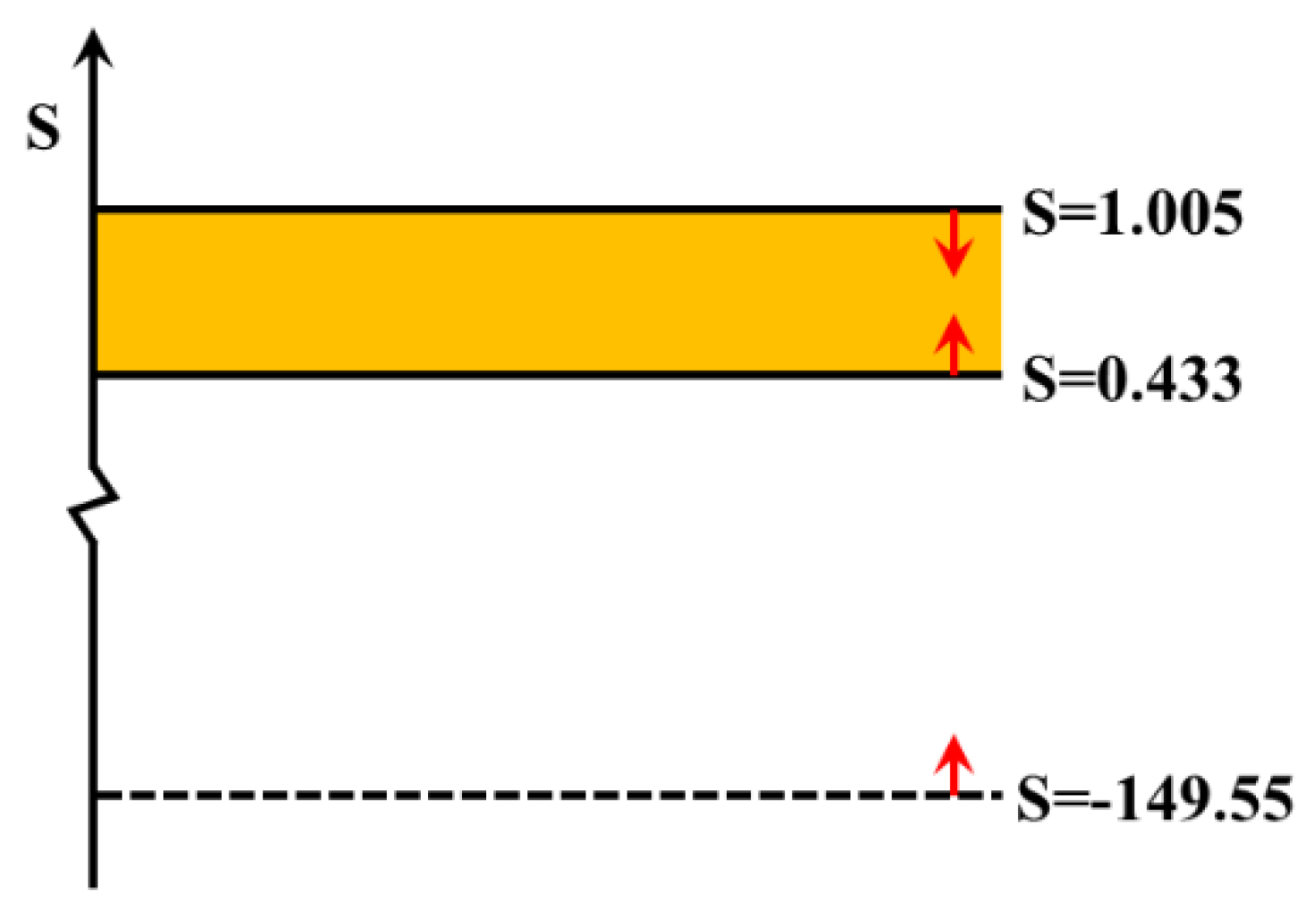
If subsidy $S$ satisfies conditions Equations (23)–(25) at the same time, $x,y,z$ will all gradually converge to zero. This means that the three parties will adopt a cooperative strategy. In the scenario of Encarnação et al. [19], public, private, and civil sectors will be in favor of electric vehicles. We selected a set of data (see

Table 1. Initial values of variables.

$\mathit{\delta }$	${\mathit{C}}_{\mathit{i}}$	$\mathit{\rho }$	$\mathit{b}$	$\mathit{i}$	${\mathit{P}}_{\mathit{b}}$	$\mathit{P}$	$\mathbf{\Delta }1$	$\mathbf{\Delta }2$	${\mathit{Z}}_{\mathit{s}\mathit{i}\mathit{z}\mathit{e}}$	$\mathit{\gamma }$	$\mathit{x}$	$\mathit{y}$	$\mathit{z}$
0.8	0.1	0.5	0.8	0.6	0.9	3	0.51	1	5	0.9	0.5	0.5	0.5

) to solve the range of subsidy $S$ by Equations (23)–(25). The boundary of subsidy $S$ we finally got was $0.433\le S\le 1.005,$ as shown in Figure 1.

In reality, the boundary of subsidy $S$ represents the range of subsidy regulation that the public sector (government) can take. Within this range, government subsidies will achieve the same effect. Therefore, if the minimum value of subsidies is smaller, the less subsidy the government can use to achieve the same desired effect. It also means the more effective the government’s regulation will be.

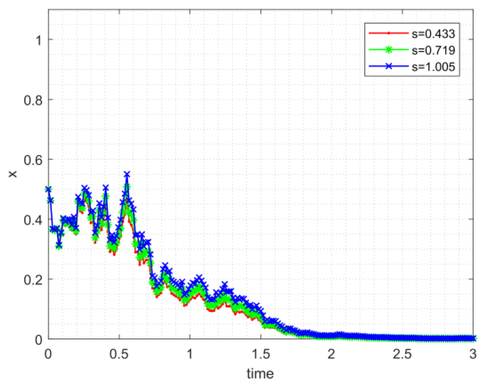
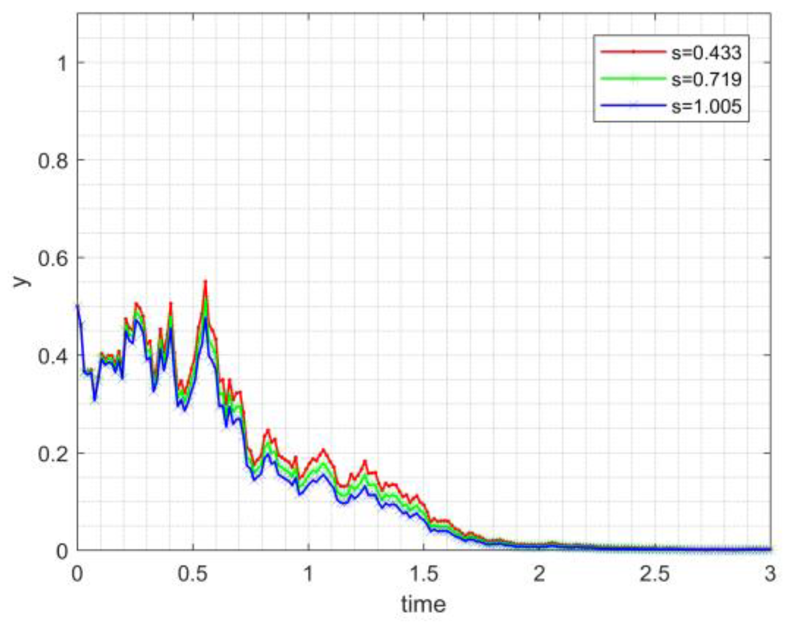
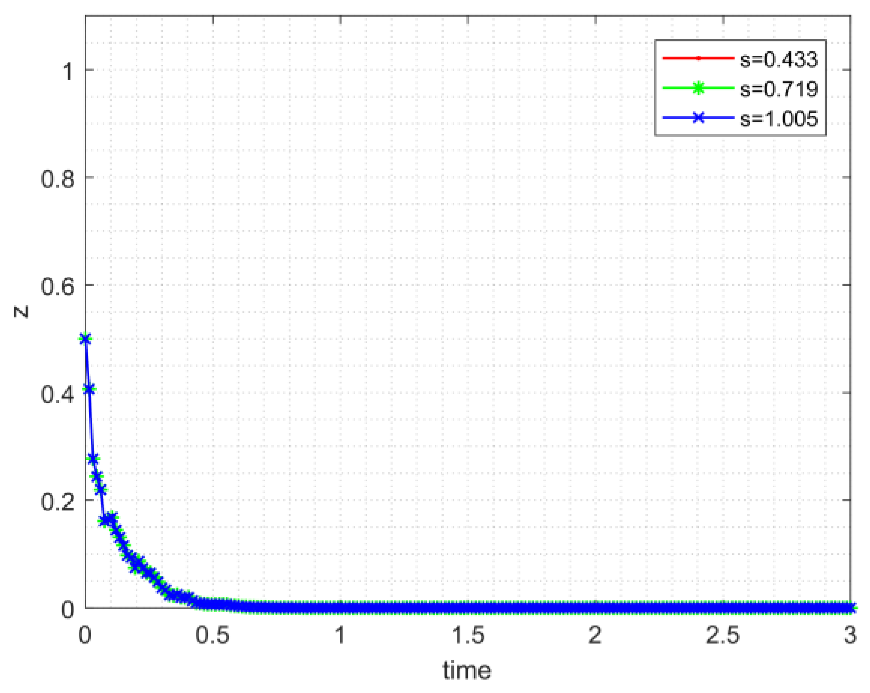
As is shown in Figure 2, Figure 3 and Figure 4, if the trivial solution of Equations (13)–(15) is p-th moment exponentially stable, then $x,y,z$ will gradually converge to zero at a speed of exponential function. In Figure 2, Figure 3 and Figure 4 results also verify the validity of the constraint.

Subsequently, we analyzed the effect of variable combination. When multiple variables change simultaneously, the change of subsidy boundary can be observed. The situations of two variables (lines 1–14,

Table 2. Initial values of variables.

	$\mathit{\delta }$	${\mathit{C}}_{\mathit{i}}$	$\mathit{\rho }$	$\mathit{b}$	$\mathit{i}$	${\mathit{P}}_{\mathit{b}}$	$\mathit{P}$	$\mathbf{\Delta }1$	$\mathbf{\Delta }2$	${\mathit{Z}}_{\mathit{s}\mathit{i}\mathit{z}\mathit{e}}$	$\mathit{\gamma }$	$\mathit{x}$	$\mathit{y}$	$\mathit{z}$	Effective Boundary and Scope of Subsidy	Range of Change	Ranking of Regulatory Effectiveness
1	0.8	0.1	0.5	0.8	0.6	0.9	3	0.51	1	5	0.9	0.5	0.5	0.5	[0.433, 1.005]	Initial group
2	0.88	0.11													[0.431, 0.995]	−0.5%, −1%	18
3	0.88	0.1	0.55												[0.410, 0.995]	−5.3%, −1%	9
4	0.88		0.5	0.88											[0.377, 1.041]	−12.9%, 3.6%	5
5	0.88			0.8	0.66										[0.415, 1.005]	−4.2%, 0%	11
6	0.88				0.6	0.99									[0.319, 1.005]	−26.3%, 0%	1
7	0.88					0.9	3.3								[0.415, 1.305]	−4.2%, 29.9%	14
8	0.88						3	0.56							[0.415, 0.980]	−4.2%, −2.5%	10
9	0.88							0.51	1.1						[0.362, 1.005]	−16.4%, 0%	4
10	0.88								1	5.5					[0.415, 1.005]	−4.2%, 0%	11
11	0.88									5	0.99				[0.377, 1.041]	−12.9%, 3.6%	5
12	0.88										0.9	0.55			[0.450, 1.005]	−3.9%, 0%	15
13	0.88											0.5	0.55		[0.415, 1.128]	−4.2%, 12.2%	13
14	0.88												0.5	0.55	[0.691, 0.767]	59.6%, −23.7%	19
15	0.88	0.11	0.55											0.5	[0.425, 0.984]	−1.9%, −2.1%	17
16	0.88	0.1	0.5	0.88	0.66										[0.377, 1.041]	−12.9%, 3.6%	5
17	0.88			0.8	0.6	0.99	3.3								[0.319, 1.305]	−26.3%, 29.9%	2
18	0.88					0.9	3	0.56	1.1						[0.362, 0.980]	−16.4%, −2.5%	3
19	0.88							0.51	1	5.5	0.99				[0.377, 1.041]	−12.9%, 3.6%	5
20	0.88									5	0.9	0.55	0.55		[0.450, 1.128]	−3.9%, 12.2%	16

) and three variables (lines 15–20, Table 2) changing at the same time are arranged in Table 2. This paper only lists two cases, and more variable combinations can be further discussed. Besides, the initial value of variables are shown in Table 1. Variable change was uniformly set to increase by 10%.

Table 2 shows the effective boundary range and the change range of boundary, respectively. (The initial values are arranged in the first row of Table 2.) If the value of the effective subsidy boundary was reduced, the parameter was marked in blue, and if it was increased, the parameter was marked in red. The goal of public sector regulation is to provide as few subsidies as possible and to ensure that the three participants are willing to cooperate at the same time. It will consider the lower limit of effective subsidy when comparing the effects of variable combinations firstly (the lower limit means the minimum effective subsidy provided by the government). The upper limit of effective subsidy is only compared when the lower limit is the same. Hence, the effects of different combinations of variables are compared in Table 2. The penultimate column in Table 2 shows the change proportion of effective subsidy range after adjustment of variable value. The greater the reduction of the minimum value, the greater the reduction in public subsidies, which also means that the regulatory goals of the public sector have been achieved.

As shown in Table 2, compared with other variables, the effect of regulating variables $\delta$ and $P_b$ is the best. Under the condition of keeping the upper limit of effective subsidy unchanged, adjusting these two variables can reduce the lower limit of effective subsidy by 26.3% (Compare lines 6 and 17 in Table 2.) In this way, we graded the regulatory results of each group of variables in the last column of Table 2. The government can quantitatively consider control measures for policy applications.

4. Conclusions

This paper proposes an improved evolutionary game model method, which considers the random turbulence in the game system. The model can analyze the conditions of players’ adoption of cooperation strategy. The article further solves the problem of the effective boundary of public innovation subsidies. The proposed improved EG model can more accurately analyze the effective range of any variable that affects the multisector cooperation and provides quantitative guidance for the supervision of the public sector.

In the case of any kind of competitive and cooperative system, there are many internal and external disturbance factors affecting the players’ strategy selection. The advantage of stochastic evolutionary game is that it cannot only reflect the interaction (competition and cooperation) between multiple players, but also consider the interference of game system. Then the stability criterion theorem can be quoted to solve the effective boundary conditions of strategy stability. Taking subsidies as an example, this paper solved the effective boundary conditions of subsidies that promote the cooperation of three populations. What is more, we can discuss the boundary conditions of any variable.

Two further research directions can be drawn from this study: First, boundaries of variables other than subsidies can be discussed and, second, the influence of different variables on strategy adoption can be analyzed.