Convolutional Attention Network with Maximizing Mutual Information for Fine-Grained Image Classification

Abstract

Fine-grained image classification has seen a great improvement benefiting from the advantages of deep learning techniques. Most fine-grained image classification methods focus on extracting discriminative features and combining the global features with the local ones. However, the accuracy is limited due to the inter-class similarity and the inner-class divergence as well as the lack of enough labelled images to train a deep network which can generalize to fine-grained classes. To deal with these problems, we develop an algorithm which combines Maximizing the Mutual Information (MMI) with the Learning Attention (LA). We make use of MMI to distill knowledge from the image pairs which contain the same object. Meanwhile we take advantage of the LA mechanism to find the salient region of the image to enhance the information distillation. Our model can extract more discriminative semantic features and improve the performance on fine-grained image classification. Our model has a symmetric structure, in which the paired images are inputted into the same network to extract the local and global features for the subsequent MMI and LA modules. We train the model by maximizing the mutual information and minimizing the cross-entropy stage by stage alternatively. Experiments show that our model can improve the performance of the fine-grained image classification effectively.

1. Introduction

In the applications of real-world image recognition [1,2], most of the objects are fine-grained. The fine-grained categories are much more than that of the coarse ones, and it often takes domain expertise to label fine-grained images, which can substantially increase the cost [3]. As a result, there are not enough labelled images to train a good fine-grained image classifier. Besides, there is the imbalance dataset problem, where a few categories have most of the images while other categories have only few images, in some real-world applications. This problem leads to the model observing rarely the categories with small number of images, resulting in a poor performance on these categories. Furthermore, in fine-grained image classification settings, due to the problems of scales changing, different viewpoints, occlusions and complex backgrounds, objects within the same subordinate class may present a lot of appearance variations while objects from different subordinate class may present similar appearances [4]. As a result, it remains a very challenging problem to recognize the fine-grained categories.

The fine-grained image classification receives increasing attention [3,5,6,7,8] benefiting from the advantages of deep learning techniques [9,10,11,12]. Different kinds of approaches are proposed to extract the subtle discriminative features to alleviate the problems of scales, viewpoints, occlusions and complex backgrounds. The general convolutional neural networks (CNNs), like VGG net [12], the GoogLeNet [10,13] and Resnet [9], are proved to be able to extract powerful generic descriptors for fine-grained image classification [4]. The features extracted by the general CNNs contain the global information of the whole image, including the foreground object and the the background clutter. However, it is believed that the semantic part features can facilitate fine-grained image classification by isolating the subtle appearance difference of the specific parts. The part localization which aims to find the discriminative parts in an object is therefore important for alleviating the classification challenges arising from the object pose variations and camera view position changes. Some approaches [14,15] have been proposed to learn the part-based representations extractor using the manually-labelled bounding box annotation. The heavy human involvement makes part definition and annotation more expensive and subjective, which in return, leads to significant progresses in methods of learning weakly-supervised part model with category labels. Some part localization methods [16] tried to utilize unsupervised methods, for example clustering, to obtain the region with higher response in the image by analyzing the features taken from different channels and take these clustering channels as parts of the images, whereas some other methods [17,18,19] tried to utilize the attention mechanism to find the discriminative parts, in which they utilize the compatibility of the global features and the local features to find the salient regions of the image. Ensemble of networks based approaches are also widely used to extract the subtle features in the fine-grained image classification systems. For example, some methods [16,20] utilized multiple CNNs to improve the fine-grained classification performance. Apart from these methods, some approaches try to leverage external information such as multi-modality data. Literature [21,22,23] proposed to map the image features to a rich semantic embedding space which is learned from the structured knowledge bases or unstructured text.

There are also many other approaches trying to solve the imbalance dataset problem in real-world applications. Imbalance of number of samples in each category could affect the fine-grained image classification. Recently, methods for oversampling the training set have been used to solve this problem. Sundaram et al. [5] proposed a fine-grained image clustering method balancing the dataset by using Synthetic Minority Oversampling Technique (SMOTE), in which synthetic images are obtained from every original image by random interpolation with some other selected neighbors from the same class. Instead of estimating the implicit multivariate probability density function, Salazar et al. [24] proposed to alleviate the problem by incorporating the structural information of the original data to the synthetic ones, which combined the Generative Adversarial Networks (GAN) with the vector Markov Random Field. Cui et al. [25] proposed a simple two stage learning approach. In the first stage, they trained a model on large amounts of training data. In the second stage, they fine-tuned on an evenly-distributed subset to gain the network’s ability to balance among all categories. The evenly-distributed subset is obtained by oversampling the categories with a small amount of images and down-sampling the categories with a large amount of images.

Existing literature provide a broad view and possibilities for fine-grained image classification. However, for practical considerations, a desirable model should be capable of finding and representing the slight visual differences between subordinate categories with limited labelled images. To solve the problems in the fine-grained image classification task and learn a desirable model, we adopt the Mutual Information (MI), which is used to measure the correlation of vectors, to measure the similarity between the features of two images and train a network to maximize it. This operation can not only promote the learned features to contain the subtle characteristics of the object, but also reduce dependence on the amount of labelled images because the paired images used for training can be generated by transforming the same image. Besides, we take advantage of the Learning Attention (LA) to find the salient region of the image so as to enhance the learning of discriminative features for each object. The motivation for combining MMI and LA is the complementary extracting ability on object semantic information. The MMI is good at extracting the semantic features without labelled images, an ability which is demanded in the fine-grained image classification due to the limited amount of labelled images in each class. Meanwhile, the attention is typically used in the image classification problem to extract salient object information, and the learned attention applied to image classification is effective in extracting diverse and complementary features.

In this paper, we design a novel joint framework for fine-grained image clustering and classification combining the MMI and LA. We assume that there is a class center for each class in the feature space and the class center will not change. The classifier directly maps the input images to the class center in the feature space, while the clustering works to map the input image pair to be closer to each other. If we set the number of the clustering to the number categories and train a common feature extractor for the different clustering and classification tasks, the function of the clustering and the classification will work in the same target of extracting the robust features to distinguish different categories. Therefore, the proposed model integrates MMI, LA with the Minimizing Cross-Entropy (MCE) modules together to enhance the performance of the network. The MMI module consists of an MI estimating function which works as an unsupervised objective. Specifically, the MMI module maximizes the mutual information of the input image pair, which contain objects from the same class, and facilitates the model to learn the discriminative features by exploiting the inner class semantic consistency with unlabelled image pairs. The LA module consists of a compatibility score estimating layer which acts as a part searcher to find the salient regions of the image. The MCE module consists of a Cross-Entropy (CE) loss which exploits the image labels to learn a image classifier and complete the final category assignment.

Figure 1 provides an overview of the proposed method, and the three different modules are marked with rectangles in the figure. We can see that our model has a symmetric structure, and it takes image pair which contains the same object as input and produces local features from the middle convolution layer as well as the global features from the first fully connected layer (Fc1). The top pipeline of the model shares the parameters with the bottom one, which means, there is only one backbone network in our model. In the MMI module, we make use of the global features of the image pair to compute the mutual information loss. The global features are converted to the semantic probability corresponding to each class in the second fully connected layer (Fc2) and the semantic probability is used to compute the mutual information of the input paired images. In the MMI module in Figure 1, z and $z^{\prime }$ represent the class assignment variables and $P(z,z^{\prime })$ represents the joint distribution which will be discussed in Section 3.2. Meanwhile, in the LA module, the global features are used to estimate the attention map of the local features and we utilize the estimated attention map to choose discriminative features from the local features. This is conducted by using the estimated attention to weight local features. Besides, in the MCE module, the chosen features are used to compute the cross-entropy loss and complete the category assignment.

The main contribution of this paper is that we propose a novel classification model which combines the traditional classification loss with the unsupervised clustering loss. The proposed model has several promising properties: (1) The model can efficiently recognize the fine-grained image with only image level labels. (2) The model takes advantage of the consistency of the object’s appearance to reduce the dependence on large amounts of labelled images to train a deep network. (3) By finding the salient regions of the image the model reduces the disturbance of the background. (4) Moreover, the model improves the fine-grained image classification accuracy by extracting discriminative semantic features. The proposed method is compared with several models on the public fine-grained image classification problems and achieve competitive results in comparison with the state-of-the-art.

The rest of this paper is organized as follows: Section 2 discusses related work. The problem formulation and the details of the proposed model are presented in Section 3. Experiments on public datasets are shown in Section 4. Section 5 concludes the paper.

2. Related Work

Fine-grained Image Classification aims to distinguish objects from others in the subordinate-level categories, e.g, different species of birds [4,26]. Due to the objects from different subordinate categories may have imperceptible differences which are even difficult for human to recognize, most approaches give up utilizing the general convolution neural network (CNN) features to classify the fine-grained images directly. Some approaches [19] took advantage of the attention mechanism to find the most salient part of the fine-grained images to extract discriminative features [4]. The attention based methods are usually pure and decent, and can be easily adopted to many others similar tasks, such as image classification and domain adaptation. Zheng et al. [16] proposed multi-attention convolution neural network (MA-CNN) for fine-grained recognition and achieved promising results in many fine-grained classification datasets. Jetley et al. [19] proposed an end-to-end trainable attention module which can be embedded into any CNN architectures built for image classification. The module can learn the attention map so as to highlight the regions of interest while suppressing irrelevant background cluster. The learned module is demonstrated to be able to bootstrap standard CNN architectures for the task of image classification. These methods can learn the attention map very well when there are enough training images, which is impractical in fine-grained image classification task, especially for real-world applications. Since it is hard and expensive to get large amounts of labelled fine-grained images.

MI plays an important role in quality of the representation in generative models [27,28,29]. However, MI is difficult to compute in continuous and high-dimensional settings. Many researchers utilized a very similar estimator to approximate the MI between high dimensional input and output pairs of deep neural network [30,31]. Hjelm et al. [31] declared that maximizing the MI between the complete input and extracted feature is often insufficient for learning useful representations, while maximizing the MI between the representation and local regions of the input e.g, patches rather than the complete image, can greatly improve the quality of the representation for classification task. Ji et al. [32] took advantage of maximizing the MI between the semantic representations of two images from the same class and proposed an unsupervised image clustering algorithm which can train a randomly initialized convolution neural network into a classification function end-to-end with only unlabelled data samples. The convolutional network is trained by Maximizing Mutual Information (MMI) of the network outputs from paired input images, which could encourage the distillation of the common part while ignoring disturbance of the background. The MMI operation was formulated as a module which can be inserted into any end-to-end learning network.

3. Method

Our model consists of Learned Attention module (LA), Max Mutual Information (MMI) module and Minimize Cross-Entropy (MCE) module. The LA module introduces an attention mechanism to ensure that the model has the ability to pay attention to the salient region of the object in the image. The MMI module makes use of unlabelled image pair to promote the feature extractor learning. The MCE module trains the classifier to classify the object by minimizing the CE.

3.1. The Learned Attention Module

The introduction of LA module is based on the observation that there is often a large region of confusing background in training images except the object. Objects from different categories may appear in the same scene, resulting in the same backgrounds. Objects from the same category may appear in different scenes, resulting in different backgrounds. The redundant background information is not only useless for object classification, but also causes a lot of disturbance. Thus we hypothesize that there is benefit to amplifying the influence of the salient image regions, meanwhile suppressing the irrelevant and potentially confusing information in other regions. In this paper, we propose to take advantage of the learned attention to find the salient image regions and amplify their influence.

The LA module is built based on enforcing the compatibility between the global features and the local features to exploit the spatial information of the different pixel position. The global features are vectors extracted from the output of the final fully convolutional layer. The local features are vectors extracted from the intermediate feature maps at each spatial pixel position after the 7th, 10th, 13th convolutional layers. We denote the global feature vector as g and the local feature vectors as L. Then we get $L=\{l_1,l_2,\cdots ,l_n\}$. Here, $l_i$ denotes the vector extracted from the output activation at the spatial location i, and n denotes the number of total spatial locations in the activation. Then the compatibility function can be defined as follows:

$${\displaystyle c_i=<u,g+l_i>,i\in \{1\cdots n\}.}$$

(1)

We simply combine the global and local features using an addition operation, and then we learn a single fully connected layer mapping from the resultant descriptor to the compatibility scores. Here, the weight vector u can be interpreted as finding the salient regions relevant to the object categories. In that sense, the weights may be seen as learning the attention map of the images. If the dimensionality of g and $l_i$ are different, supposing $C_2,C_1$ respectively, we learn a dimension expand project function to map $l_i$ to the dimensionality of g, and we get the new local feature $\widehat{l_i}$ with dimension of $C_2$. For the local layer, we can get the set of compatibility scores $C(\widehat{L},g)=\{c_1,c_2,\cdots c_n\}$, where $\widehat{L}$ is the new local features under the linear mapping of the $l_i$ to the dimensionality of g.

The compatibility scores can be normalized in various ways, of which softmax function and sigmoid function are the most used ones. Because the softmax function has a very strong effect on emphasizing primary features and suppressing the secondary features. Using it will rely too much on the one salient part of the object. We believe that it is not enough to utilize only one certain part features of the object in fine-grained classification, and we should make full use of all available part features. As a result, we normalize the compatibility scores by the sigmoid function to obtain the final attention map:

$${\displaystyle a_i=\frac{1}{1+exp(-c_j)},i\in 1\cdots n.}$$

(2)

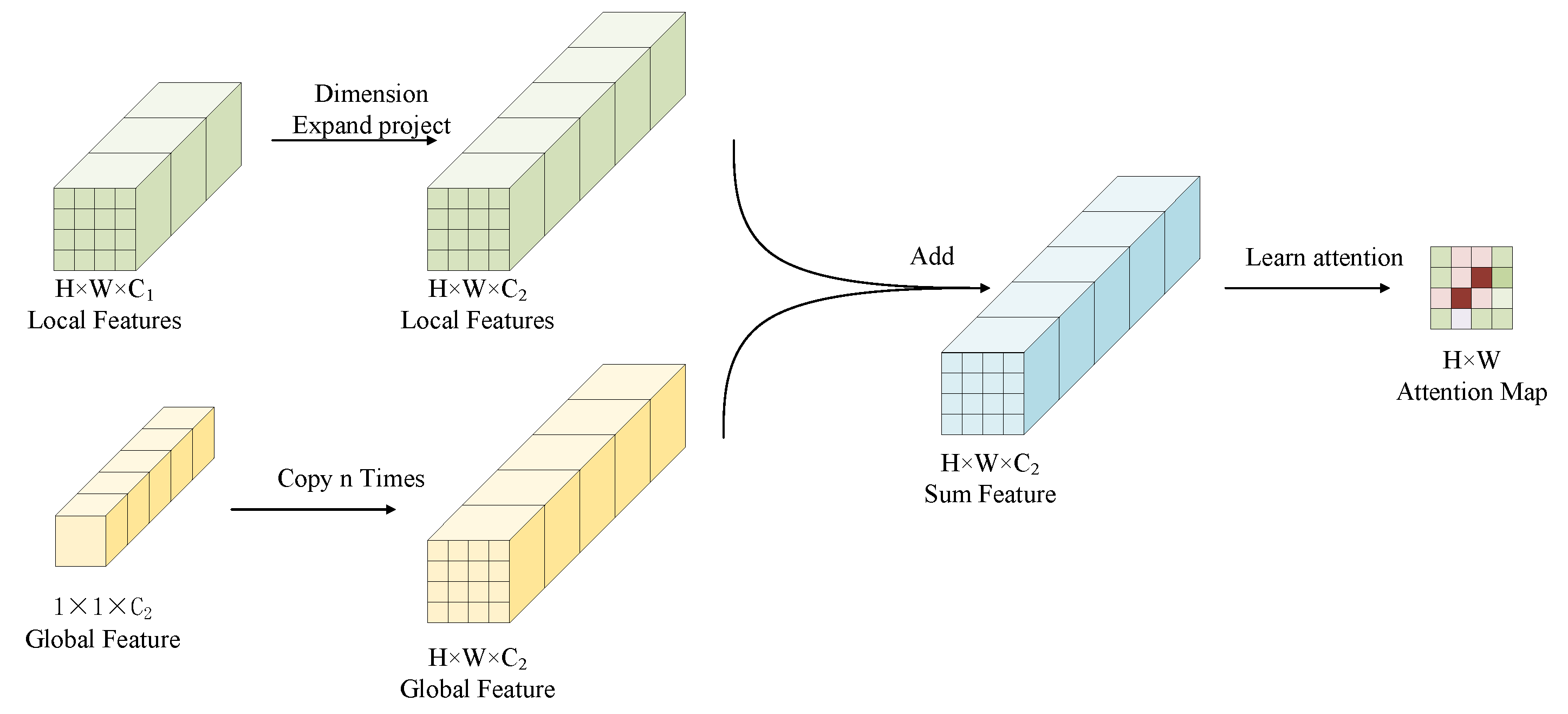
The attention calculation process is shown in Figure 2. In the left part, when the dimensionality of the local features are different from the global one’s, the local features with shape of $H\times W\times C_1$ are projected to the one with shape of $H\times W\times C_2$. Here, $C_2$ is the dimensionality of global features. In order to facilitate computing process in the GPU device, we copy the global feature $n(n=H\times W)$ times to construct feature tensor with shape of $H\times W\times C_2$. We combine the new local features with the global features by an addition operation, and the sum features are used to learn the $H\times W$ compatibility scores. After we normalize the compatibility scores, we get the attention map $A=\{a_1,a_2,\cdots a_n\}$.

The attention map A is then used to weight the feature vector in every pixel position. The weight matrix A can be interpreted as choosing the salient regions of the image and amplifying them. We get the a feature vector $g_a={\sum }_{i=1}^n{a}_i{\dot{l}}_i$ for local feature L and $g_a$ could be used as the final image feature for the classification. As is known to all, different layer extracts different level of features in the CNN. As deeper as it goes, the CNN extracts features changing from low level features like edges, shapes, colors and textures, to high level features like the parts and class semantic features. To take advantage of multi-layer features, we first concatenate the attention weighted features from different layers into a single vector and then input it to the linear classification function.

3.2. The Maximizing Mutual Information Module

The introduction of MMI module is because that there are not much labelled training images in the fine grained image classification task and MMI can take use of the unlabelled image pairs to train a classifier end-to-end. We denote the paired images which contain the same object as $x,x^{\prime }$. The MMI module can be formulated as maximizing the mutual information between the projections of the related pairs:

$${\displaystyle \underset{\Phi }{max}I(\Phi \left(x\right),\Phi \left(x^{\prime }\right)).}$$

(3)

where $\Phi$ is the feature extracting network. As claimed by Ji et al. [32], when $\Phi$ represent a network with a small output capacity, which is often called a bottleneck, maximizing the MI between the encoded variables could have the effect of learning a feature extractor $\Phi :x\to g$ that preserves the common part between x and $x^{\prime }$ and discards the image specific details, such as the background. The problem described in Equation (3) is hard to resolve, because MI is notoriously difficult to compute, particularly in continuous and high-dimensional settings [13].

Fortunately, in the classification setting, the class space $y=1,\dots ,C$ is discrete and the number of classes C is limited. We can compute the MI exactly. Assuming that we have a trained classification network $\Phi$ and a pair of input images x and $x^{\prime }$, which contains the same object, such that we will get the outputs $o=\Phi \left(x\right)$ and $o^{\prime }=\Phi \left(x^{\prime }\right)$ of the two input images. To solve Equation (3), we need to compute the joint distribution of o and $o^{\prime }$ as well as the marginal distribution of o and $o^{\prime }$ respectively.

Because the output of the network is normalized by a softmax function, we have $o=\Phi \left(x\right)\in {[0,1]}^C$ and output o can be interpreted as the distribution of the image x over classes in the class space, which can be denoted by $P(z=c|x)={\Phi }_c\left(x\right)$. Here z and $z^{\prime }$ are referred to as a class assignment variable. The conditional joint distribution of z and $z^{\prime }$ is given by $P_{c{c}^{\prime }}=p(z=c,z^{\prime }=c^{\prime })={\Phi }_c\left(x\right)·{\Phi }_c^{\prime }\left(x^{\prime }\right)$. Therefore, the joint probability distribution of o and $o^{\prime }$ over classes can be calculated by marginalization over the dataset:

$${\displaystyle \mathbf{P}=\sum _{i=1}^N\Phi \left(x_i\right)·\Phi {\left(x_i^{\prime }\right)}^{\top },}$$

(4)

where N is the number of image pairs, and the $C\times C$ matrix $\mathbf{P}$ is constituted of ${\mathbf{P}}_{c{c}^{\prime }}$ at row c and column $c^{\prime }$. Then we compute the marginal distribution ${\mathbf{P}}_c=P(z=c)$ and ${\mathbf{P}}_{c^{\prime }}=P(z^{\prime }=c^{\prime })$ by summing over the rows and columns of $\mathbf{P}$. The objective function in Equation (3) can be easily computed using the following formula:

$${\displaystyle I(o,o^{\prime })=\sum _{c=1}^C\sum _{c^{\prime }=1}^C{\mathbf{P}}_{c{c}^{\prime }}·ln\frac{{\mathbf{P}}_{c{c}^{\prime }}}{{\mathbf{P}}_c·{\mathbf{P}}_{c^{\prime }}}.}$$

(5)

To insert the MMI module into an end-to-end trainable network which can be optimized by the stochastic gradient descend [33] method, we re-formulate the Equation (5) as:

$$M{I}_{Loss}=-\sum _{c=1}^C\sum _{c^{\prime }=1}^C{\mathbf{P}}_{c{c}^{\prime }}·ln\frac{{\mathbf{P}}_{c{c}^{\prime }}}{{\mathbf{P}}_c·{\mathbf{P}}_{c^{\prime }}}.$$

(6)

The specific process to calculate the MI loss is shown in Algorithm 1.

Algorithm 1: Calculate the MI loss

MMI module requires a set of paired images $(x,x^{\prime })$, which are easy to generate in the supervised classification. While in the limited labelled image situation, we can also apply transformation method to generate the image pairs, which consist of image x and its randomly transformed version $x^{\prime }=T\ast x$. T represents a set of transformation functions, including normalization, scaling, rotation, random cropping, color saturation and contrast changing, which are often used in deep learning model to augment data while preserve the key content of the image. Then the MMI can be used to dig out the invariant content between the image pairs and map the paired images to the same class center.

3.3. The Minimizing Cross-Entropy Module

While the proposed model can help detect salient region and extract the image features with the unlabelled images by simultaneously utilizing LA and MMI module, the classifier learned is not good enough to complete the category assignment, which is because the classifier learned by MMI can only produce different images clusters. In order to train a classifier to complete the category assignment, we design the MCE module. The CE and the Mean Square Error (MSE) criteria are the most popular choices in state-of-the art implementations during the training of CNNs. The CE criterion has been proved to be able to find a better local optimum than Square Error criterion, which often results in the gradient vanishing early and no further reduction of classification errors possible [34]. In practice, CE can lead to faster convergence and better results in most classification tasks. Thus, we follow the tradition of image recognition and make use of the CE as our criterion. In the MCE module, the classifier is formulated as a FC layer and we train it with the CE loss as the objective.

$${\displaystyle C{E}_{Loss}=-\sum _{c-1}^C{y}_{c}ln\left(p_c\right).}$$

(7)

3.4. Convergence and Computational Complexity Analysis

It is well known that the optimization of CNNs is a non-convex problem and it is hard to fully-understand the convergence for finding the approximate critical points of a non-convex function [35]. However it becomes easier for a randomly-initialized CNN to avoid the local minima, and it is proved that the stochastic gradient descent (SGD) [33] can find global minima on the training objective of CNNs in polynomial time [36] if the inputs of the network are non-degenerate and the CNN is over-parameterized. The former means that the same input sample should have the same label, while the latter means that the network should have much more parameters than the numbers of the training samples. This is the very condition of the proposed model. Our model is composed of the standard convolutional layers as well as the FC layers and is an over-parameterized network. Each image in our datasets has only one specific class label. Thus, we assume that the model will find the global minima in the proper parameters setting.

The computational complexity of MMI module is $O\left(C^2\right)$, where C is the number of classes. The LA module and the backbone network consist of convolutional layers and FC layers, The total computational complexity of a convolution layer’s one forward propagation is $O(h_{l-1}^2\times K^2\times h_l^2\times m_l^2)$. Here l is the index of a convolutional layer. $h_{l-1}$ and $h_l$ are known as the number of input and output channels of the l-th layer. K is the spatial size of the kernel. m is the spatial size of the output feature map. According to [37], this time complexity also applies to backward propagation, because the training time per image is roughly three times of the testing time per image. The input and output features of FC layer are one dimension vectors. The computational complexity of one FC layer is $n_1\times n_2$, where $n_1$ is the length of the input feature and $n_2$ is the length of the output feature. The length of the output feature from the last layer is C. We denote the size of the input image as $H\times W$. When the network is fixed, the computational complexity of the network is $O(H\times W\times C)$.

At the training phase, optimizing CNN using SGD algorithm is time-consuming. It needs repeated iteration of forward and backward propagations through the whole network. Multiple graphics processing units (GPU) are used to accelerate the computation. For the Caltech-UCSD Birds-200-2011 (CUB) dataset, the training time for one iteration is 18 ms per iteration, While at the inference stage, the recognition speed is very fast and the runtime of class prediction is 3 ms per iteration.

4. Experiments

To evaluate the performance of the proposed framework, we conduct experiments on three challenging datasets, including the datasets CIFAR-10 and CIFAR-100 [38] for image classification as well as the Caltech-UCSD Birds-200-2011 (CUB) [39] dataset for fine-grained image classification. The performance is compared with several baseline methods, including The VGG [12], The GOOGLE-GAP [13], The RN34 [40], Inception-v3 [10] and LPA [19]. The experiments are carried out on a PC with a 4.0 GHz Intel(R) Core(TM) i7-4790K CPU, 16GB RAM and a NVIDIA(R) GeForce(TM) GTX TITAN Xp GPU. The top-1 error is used to evaluate the performance of the proposed model.

4.1. Dataset and Baseline Methods

The CUB is a widely-used challenging fine-grained image classification dataset, of which the images are collected using Flickr image search and filtered by multiple special workers. The CUB dataset contains 11788 photos of 200 bird species from North American, including 5994 training and 5794 test images. Samples of the first six classes of the dataset are visualized in Figure 3. The six images in each row are sampled from the same category, and the category name is present at the left of each row. It can be seen that due to different viewpoints, different environments, and different scales, the images in the same row seem very different, while images from different rows may present more similar appearance. For example, in the image preprocessing stage, besides the contrast normalization, we make use of many other forms of data augmentation including random flipping and random cropping. During the train stage, each image fed into the model is flipped horizontally with probability 0.5 and is cropped randomly using size on the interval [0.3,1) of the origin.

CIFAR-10 [38] is a popular dataset for small-scale image recognition. The dataset is composed of 60,000 $32\times 32$ color images from 10 classes, with 6000 images per class. The dataset is divided into 50,000 training and 10,000 testing images. We preprocess the data by subtracting the mean and dividing the standard deviation of each image vector to perform contrast normalization.

CIFAR-100 [38] is a popular dataset used for image recognition as well as fine-grained image classification. Similar to CIFAR-10, the dataset consists of 60,000 $32\times 32$ color images. Differently, the dataset has 20 coarse labels and each of them has 5 fine labels. For example, There are “aquarium fish”, “flatfish”, “ray”, “shark”, “trout” in the “fish” category. We make use of the fine-grained labels to evaluate our the proposed model. As a result, there are only 500 training images for each class.

The detailed statistics with category numbers and data splits are summarized in

Table 1. The statistics of datasets used in this paper.

Datasets	#Category	#Training	#Testing
CUB	200	5994	5794
CIFAR-10	10	50,000	10,000
CIFAR-100	100	50,000	10,000

.

The proposed model is simply designed by adding an MI loss function and an attention learning layer to the little modified VGG network. Therefore, we choose to compare our model with the simple models with similar little modification. The baseline models in the classification which adopted different popular architectures and the attention mechanisms are chosen as the compared methods. The VGG was the first model to successfully take advantage of the very deep convolution network to extract discriminative features. The GOOGLE-GAP enhanced the network’s localization ability by making use of the global average pooling in the GOOGLE network in which the output of global average pooling was used to weight the convolution feature map and the sum of the weighted feature maps were referred to as the class attention map. The RN34 utilized the ResNet as the backbone and improved the performance of the classification by transferring the attention model from the teacher network to the student network. The attention used in RN34 was also based on the activation, while the difference is that RN34 focused on the spatial information while the the GOOGLE-GAP focused on the information implied in the different channel. The Inception-v3 network proposed a convolution factorizing method which factorized the convolutional layer with large spatial filters to a multi-layer convolutional network with small spatial filters and maintained the input size and output depth unchanged. As a result, Inception-v3 network can extract richer features and increase feature diversity. The LPA utilized the global feature as a query to find the attention region in the local feature activation of the input image and combine the attention module with the VGG network in a very decent manner. Different from the attention used in our model, LPA used softmax to normalize the compatibility scores. We believe that the softmax will encourage the extracted features to exceed the maximum value on the feature map while suppress the local maximum values. However, these local maximum values also represent some important discriminative regions of objects.

4.2. Implementation Details and Training

We use the 16-layers VGG [12] network as the basenet. The VGG-16 network has 13 convolutional layers and 3 fully connected layers. Following the settings of Jetley et al. [12], we add two more convolutional layers after the last convolutional layer of the VGG-16 network, and then obtain the global features of the image by averaging the pooling layer. The local features are extracted from the output of the 7th, 10th, and 13th convolutional layers of the network. For experiments on CIFAR-10, in order to retain more detailed information of the image, we move the max-pooling layer of the first two blocks of VGG-16 to the end of the pipeline, so that the size of the first local feature layer is 16 × 16.

In order to calculate the MI of images, we need to generate image pairs containing the same object. In the fine-grained image classification setting, there are two choices: To randomly select a different image with the same label for each image from the train dataset, or to randomly obtain an image from the dataset, then generate the image pair through image transformation. For the first choice, we create a new data loader to load two different images from the same class, and then we use the same image transformation on them before inputting them into the network. For the second one, we normalize the input image to $256\times 256$ and then use different transform methods, such as random horizontal flipping and random cropping, to generate two different inputs. All the images in CUB are cropped to $224\times 224$ before inputed into the network.

All networks proposed in this paper are randomly initialized and trained from scratch. The networks are trained end to end under the constrained CE loss and the MI loss. The CE loss works as a target of training a classifier and the MI loss works as a target of training a clustering. The classifier and the clustering share the backbone in our model. We train the model by alternating between the classification training and the clustering training stage by stage. The classification training and clustering training are conducted for different times in one stage. Specifically, the clustering training is conducted for one epoch after the classification training is conducted for 10 epochs.

We train our model using the SGD optimizer. For fair comparison, we set the same parameters according to LPA [19], setting the learning rate decay of $1\times {10}^{-7}$, weight decay of $5\times {10}^{-4}$, and momentum of 0.9. In the classification training stage, the initial learning rate for CIFAR-10 experiments is set to 0.1 while the initial learning rate for CUB is set to 0.01, for the batch size of CUB dataset is very small. The batch size of CUB dataset is set to 16 due to the limitation of the GPU memory. The learning rate starts to decrease by half every 25 epochs because the learning rate annealing has been shown to increase the generalization of the network [41]. In the clustering training stage, the learning rate is set to 0.0004 for the base network as well as for the inter-image MI head.

We refer to the network implementing attention on the output of all the three levels as CANMMI-att and the three levels of attention weighted features are concatenated together as the final feature for classification. We refer to the network implementing attention on the output of the first level(layer 7), the second level(layer 10) and the third level(layer 13) as CANMMI-att1, CANMMI-att2 and CANMMI-att3, respectively.

4.3. Results and Analysis

4.3.1. Results of Evaluation on Benchmark Datasets

We compare our model with five different famous methods on backbone architectures of VGG, GoogleNet, ResNet and Inception-v3, respectively, with two of the five methods based on VGG. The fine-grained classification results on the CUB dataset are shown in

Table 2. Fine-grained classification on dataset CUB: Top-1 errors (%). * denotes results from publications.

Model	Cropped	Top-1 Errors (CUB)
VGG * [12]	✓	34.64
GOOGLE-GAP * [13]	✓	29.50
RN-34 * [40]	✓	26.5
Inception-v3 [10]	×	25.5
LPA * [19]	✓	26.8
CANMMI	×	24.5

. Note that for fair comparison, the results of the some compared methods are directly cited from their original papers and marked with asterisks in the result table. The results of Inception-V3 are reproduced using the recommended settings of parameters. From these results, we can see that the proposed model has a noticeable performance improvement over the none-attention model VGG by 11.14% and outperforms the attention weighted VGG model LPA by 2.3% in top-1 errors, which shows that the features learned by the attention module and the MMI module are more discriminative for classification. Within the standard VGG architecture, we utilize the similar attention mechanism with LPA. The only difference is that the proposed model take advantage of MI loss in the training stage and the sigmoid normalization of the compatibility scores. We believe that the 8.58% improvement over LPA the proposed model achieves can be attributed to the incorporation of the MI and LA modules. Compared with other wide and deep architecture, our proposed model also has some advantages. The proposed model achieves 5.0% improvement over GOOGLE-GAP and achieves 2.0% improvement over RN-34 in top-1 errors. Inception-v3 is an update version of GOOGLE network which is also referred to as Inception-v1. We can see that Inception-v3 achieves a better performance than GOOGLE-GAP and many other methods. This is because the convolution factorizing design enables the network to acquire larger receptive field and to increase the number of network layers. The proposed model achieves a slight performance improvement over Inception-v3 due to that our model could find the salient parts of the image. It is worth mentioning that the RN-34 and the Inception-v3 model for CUB are pre-trained on ImageNet, the LPA model is pre-trained on CIFAR-100, whereas, the proposed model is trained from scratch using the CUB images only. It is well known that there is an overlap between CUB and the ImageNet. Furthermore, for VGG, GOOGLE-GAP, RN-34 and LPA, images are cropped using the bounding box annotations to get rid of the background influence, while in the proposed model, only the original images with image level labels are used to train the proposed model.

In order to verify the generalization ability of the model to other datasets, we also conduct experiments on the image classification dataset CIFAR-10 and CIFAR-100 and the results are presented in

Table 3. Fine-grained classifications on datasets CIFAR-10 and CIFAR-100: Top-1 errors (%). * denotes results from publications.

Model	CIFAR-10	CIFAR-100
VGG * [12]	7.77	30.62
GOOGLE-GAP * [13]	9.87	31.77
RN-110 * [9]	6.43	-
Inception-v3 [10]	4.9	19.1
LPA * [19]	5.23	22.97
CANMMI	4.8	19.77

. From the table, we find that CANMMI performs comparably to existing approaches, achieving a top-1 error of 4.8% on CIFAR-10 dataset and top-1 error of 19.77% on CIFAR-100 dataset. We notice that the Inception-V3 achieves a better performance than CANMMI in CIFAR-100 by 0.6%. This is because the inception module in Inception-V3 can combine features of different resolutions, which is similar to the function of the LA module. What’s more, the Inception-V3 is trained start from the model pre-trained on ImageNet. The skip connection of the ResNet has the similar effect of connecting the local features with the global ones and the ResNet architecture based model RN-100 achieves a similar performance of 6.43% in CIFAR-10 compared to the proposed model. The CANMMI model achieves an improvement of 5.0% and 12% over the GoogleNet architecture based attention network for CIFAR-10 and CIFAR-100, respectively. Despiting using the same backbone, the proposed model has a performance improvement over the baseline VGG by 2.9% and 10.85% for CIFAR-10 and CIFAR-100, respectively. The improvements over LPA the proposed model achieved suggest that the MMI has a good enforcement on the classification performance.

In order to display the contribution of features from different layers to the class prediction, we conduct experiments to adopt different level of features to predict the image class separately. The experiments are conducted on the same settings as the one using concatenation of all the three levels features. The results are shown in

Table 4. Fine-grained classification on dataset CUB: Top-1 errors (%).

Model	Top-1 Errors (CUB)
CANMMI-att1	60.6
CANMMI-att2	48.0
CANMMI-att3	24.7
CANMMI	24.5

. The model denoted by CANMMI-att1 uses the first level attention-weighted features for classification. Similarly, the model denoted by CANMMI-att2 and CANMMI-att3 make use of the second and third level attention-weighted features for classification, respectively. It can be seen that when one separated attention layer is used for prediction, the classification performance of CANMMI-att1 is not as good as that of CANMMI-att2 and CANMMI-att3. This is because although the features extracted from the low layers keep more details but they lose the main semantic information. CANMMI-att3 outperforms the other two networks a lot and has the lowest top-1 error. The combined model CANMMI-att performs slightly better than CANMMI-att3 by 0.2%.

4.3.2. Results of Quantitative Analysis

To deeper explore the discriminability of features, we visualize the features learned by the proposed model using the t-SNE embeddings [42]. We choose the first 10 classes from 200 classes on the CUB dataset for visualization and the name of the chosen classes are “Black Footed Albatross”, “Laysan Albatross”, “Sooty Albatross”, “Groove Billed Ani”, “Crested Auklet”, “Least Auklet”, “Parakeet Auklet”, “Rhinoceros Auklet”, “Brewer Blackbird”, and “Red Winged Blackbird”. After feeding the selected images into the CANMMI model, we get a set of 1536 dimension features from the output of the layer before the last softmax classification. Then we utilize the t-SNE tool to calculate the s-SNE embeddings of the features and plot them in Figure 4. In the figure, each point represents an image, and points of different colors and shapes represent different categories. We can see that the features extracted by our model are discriminative in every class on the test dataset, which suggests that the joint of attention module and the MMI module is a powerful approach to disentangle the classes from the dataset.

In Figure 5, we show some examples of the attention learned using the proposed approach. The first column shows original images, the second column shows images mixed with the 10th layer of attention map, and the third column shows images mixed with the 13th layer of attention map. We find that the proposed model enables the network to focus on the object which contains the discriminative information while suppress the background regions. As shown in Figure 5, the attention map learned by the proposed model can detect the edge of the object, and different layer learns to focus on different object parts. For example, the attention map learned in convolution layer 10 focuses on the whole body of the bird, while the attention map learned in convolution layer 13 focuses on the head of the bird, which is the most discriminative part. As a whole, we take advantage of features extracted from both layer 10 and layer 13 for the final classification.

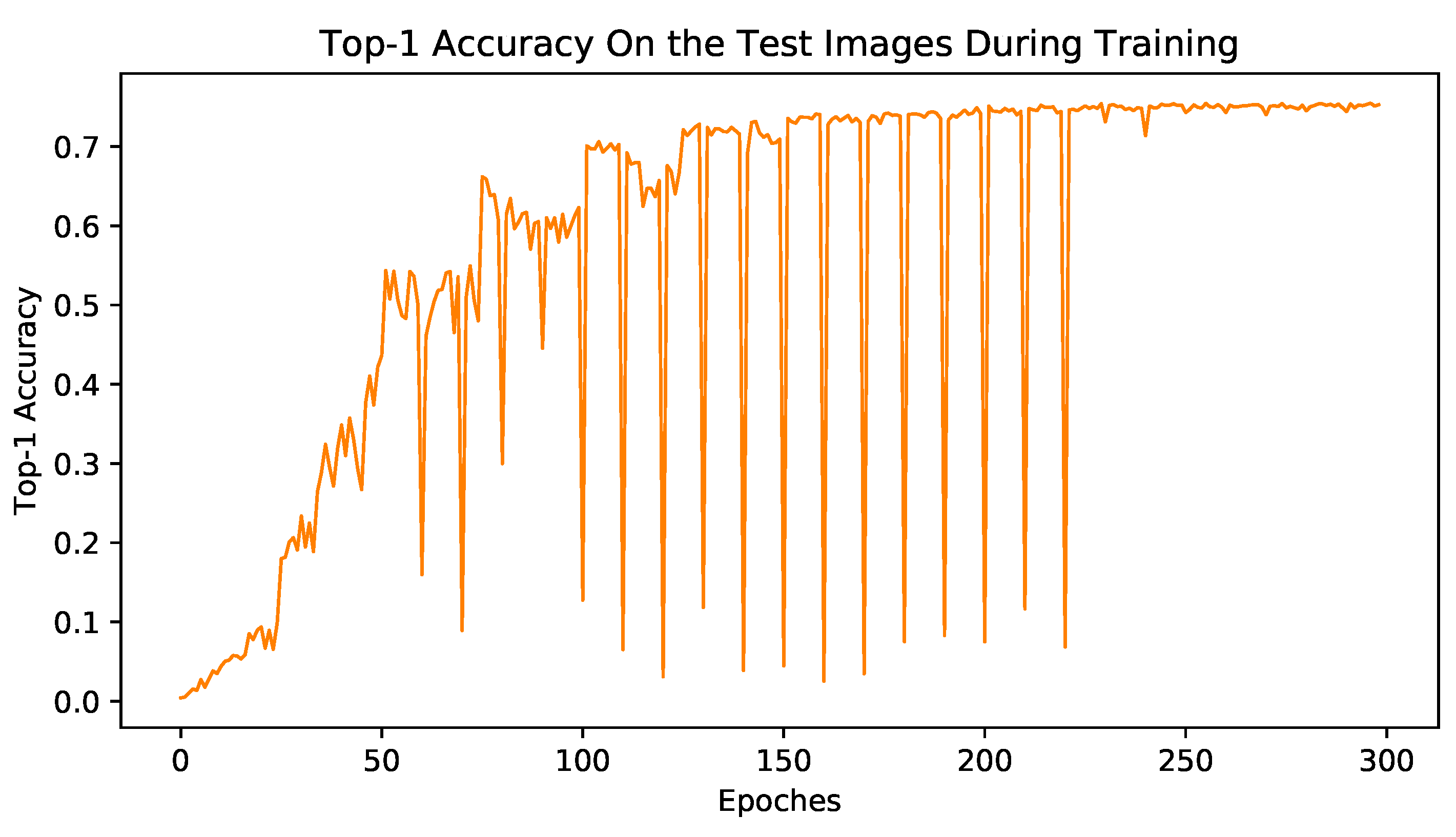
An interesting phenomenon appears when we plot the accuracy curve on the test dataset. We find that the CANMMI model could achieve a balance between maximizing MI and minimizing the CE and finally reach a stable status. The test accuracy curve is shown in Figure 6, the horizontal axis represents the training epoch, and the vertical axis represents the accuracy on the test dataset. When we alternately use CE loss and MI loss to train the model, the accuracy of the model on the test dataset shows an upward trend with fluctuations. In the pro-phase, whenever MI loss is used, the performance of the model on the test set will decrease significantly, but after a certain number of training steps, the negative impact of MI loss on the model performance gradually abates, and almost disappears in the end. While the goals of CE loss and MI loss are similar, they are quite different. The goal of MI loss is to ensure that the image features containing the same object cluster to the same class center. While the goal of CE loss is to converge image features to the corresponding position of the class orderly. However, as the training progresses, CE loss can achieve a more accurate mapping of the object to the corresponding object position, and the object position becomes the center of the clustering. The MI loss can help to make these mappings more compact, as a result, the two goals become more and more unified. Together, they promote the improvement of the model performance.

5. Conclusions

We propose an end-to-end learning model that classifies the fine-tune image without bounding box annotation. The model is built by combining minimizing CE and maximizing MI together. Minimizing the CE loss acts as a classifier learner, which is conducted on the attention weighted features. Maximizing MI acts like a clustering learner, which is helpful to extract essential characteristics of the object on paired input images. We demonstrate that the proposed model can improve the fine-grained image classification performance by using the unsupervised MMI module as well as the learning attention module. We also show that MMI can take advantage of the consistency of the objects’ appearance to alleviate the dependence on the large amount of labelled images. Further, the LA mechanism could find the salient parts of the object. The method is total data-driven and can be easily applied to different datasets. We evaluate our model on the popular fine-grained image classification dataset and achieve promising results compared with the state-of-the-art methods. In future, we will focus on investigating the mechanism of hybrid training of two different tasks and attempting to utilize the model to solve the imbalance dataset problem.