Fluid-Structure Interaction of Wind Turbine Blade Using Four Different Materials: Numerical Investigation

Abstract

The interaction of a flexible system with a moving fluid gives rise to a wide variety of physical phenomena with applications in various engineering fields, such as aircraft wing stability, arterial blood progression, high structure reaction to winds, and turbine blade vibration. Both the structure and fluid need to be modeled to understand these physical phenomena. However, in line with the overall theme of this strength, the focus here is to investigate wind turbine aerodynamic and structural analysis by combining computational fluid dynamics (CFD) and finite element analysis (FEA). One-way coupling is chosen for the fluid-structure interaction (FSI) modeling. The investigation is carried out with the use of commercialized ANSYS applications. A total of eight different wind velocities and five different angles of pitch are considered in this analysis. The effect of pitch angles on the output of a wind turbine is also highlighted. The SST k-ω turbulence model has been used. A structural analysis investigation was also carried out and is carried out after importing the pressure load exerted from the aerodynamic analysis and subsequently finding performance parameters such as deformation and Von-Mises stress.

1. Introduction

In recent years, many countries are facing a lack of traditional energy resources and the adverse effects of air pollution caused by the use of fossil fuels. Considering this fact, the government has encouraged various researchers, engineers, and entrepreneurs to work on renewable energy production while passing different legislations and providing subsidization. Many countries in Europe and Asia have substantially increased total wind power capacity and are making numerous efforts to grow the wind industry [1,2]. Increasing energy demand also raises a wind turbine’s installation capacity from kilowatt to megawatt. This constant energy demand also leads the design engineers to develop more powerful and more giant turbines in which the rotor’s diameter reaches up to 125 m [3]. Wind turbine blades are long, thin, and flexible structures that rotate and convert the kinetic energy present in the wind into mechanical energy that is further converted into electrical energy. The rotation of the wind turbine is possible through the generation of lift, and the lift occurs because of pressure distribution between the upper and lower surface of the turbines blade. This pressure distribution then adds aerodynamic loads on the surface of the blades, causing the blade to deform and bring about an aeroelastic impact. In addition, this deformation will lead to a further change in the flow area, resulting in more load changes. This aeroelastic impact, similar to a flutter, is so destructive that it brings variance in blade design and opposes the turbine in generating significant electricity. This aeroelastic issue arises due to the fluid-structure interaction (FSI), which makes FSI an investigating task for all design engineers and researchers. Therefore, proper FSI modeling is needed to meet the required standard for wind turbine development [4]. Modeling FSI requires the coupling of an aerodynamic segment and structural segment, which allows aerodynamic and structural analysis of the considered model separately. In this paper, the computational fluid dynamics (CFD) model was chosen for the aerodynamic portion of FSI modeling. Due to a high degree of accuracy and versatility, CFD attracts tremendous interest from researchers and design engineers. Due to its multifunctional features, CFD provides not only reliable results of aerodynamic coefficients but also offers minute details on flow and wake development [5,6,7,8]. According to previous studies, two approaches are used for the structural component of FSI modeling: One is the Beam model, and the other is finite element analysis (FEA) [9,10]. Between these two, Beam models are computationally efficient because they represent the three-dimensional structure in a one-dimensional form and discrete properties along the one-dimensional beam. Few researchers have investigated the aeroelastic effect by considering a nonlinear beam model [11]. The Beam model, however, failed to provide detailed information on stress distribution within the blade arrangement. However, for an FEA model, shell thickness defines the composite layer characteristics, and shell elements help build the composite blades [12]. In addition, this model has the benefits of high accuracy and can analyze the precise stress distributions in any composite layer. Therefore, this paper selects the FEA model as the structural component of FSI modeling.

Fluid-structure interaction (FSI) follows two coupling techniques. The first is a one-way coupling, and the second is a two-way coupling. The two-way coupling utilizes the results of pressure loading from the aerodynamic segment and deflection from a structural segment of FSI to get mapped until convergence is accomplished. Whereas, the one-way coupling only uses the pressure loading from the aerodynamic model to map with the structural one and get a deflection. In contrast to the latter, the former is more computationally efficient for initial analysis. Hence, the one-way coupling has been selected in this paper for fluid-structure interaction.

While designing a wind turbine blade, a twist angle and pitch angle of the blade are considered as an essential parameter. However, the pitch angle plays a vital role in determining the wind turbine’s efficiency [13,14,15]. Few researchers used the concept of tip plates to improve the wind turbine blade performance by setting the pitch angle at a maximum output power based on the given wind speed [16]. Few researchers also concentrate on varying rotor speed and blade pitch in high wind speeds. They proposed a robust sliding mode approach, where the blade pitch is considered as a control input to regulate rotor speed to a fixed rated value in the presence of uncertainties characterizing the wind turbine model [17]. As the blade pitch system needs to be monitored appropriately, few mechanisms were also proposed to reduce wear on the wind turbine pitch drive [18]. Furthermore, due to the non-linearity of wind turbine dynamics and their uncertainties, the researchers have developed various pitch control frameworks that allow the simultaneous advancement of power regulation and load mitigation via the blade pitch control [19,20]. Various methods similar to the multi-evaluated logic such as fuzzy logic and the optimization method such as a genetic algorithm, have been used to control the pitch angle by accommodating non-linearities, and this further gives stability to the wind turbine system by reducing the loading effects on the wind turbine blade [21,22].

The details of this analysis can be summarized as follows:

• In the published literature, there have been several studies that have investigated the effectiveness of the pitch angle on the HAWT output, either using just a few pitch angle values or using lower fidelity modeling. Consequently, a current understanding of how the pitch angle influences the turbine output is inadequate. The present study supplements the current information by using CFD calculations and FEA calculations that are validated against the standard empirical equations to investigate the impact of the blade pitch angle on the output parameter.
• The investigated operating conditions include five-pitch angles with increments of 4° and eight different wind speeds. No previous study has used these operating conditions to investigate the effects of pitch angles, which provides a more detailed understanding of how the wind turbine behavior changes for different pitch angles.
• In the previous literature, primarily the influence of pitch angles on the turbine output parameter has been studied. At the same time, the present research explains thoroughly how turbine blade pressures are altered in various pitch angles and wind speeds. Along with the change in pitch angle, this helps realistic assumptions to be made for the next step in the improvement of a horizontal axis wind turbine (HAWT) efficiency.
• The current study provides a comparison between the Von-Mises stress distribution of turbine blades for different pitch angles, different wind speeds, and different materials. To the best of our knowledge, this is the first study to report the pitch angle effect on Von-Mises stress distribution.
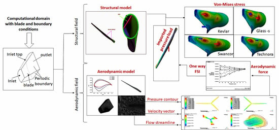
• Although the one-way fluid-structure interaction has been performed for the wind turbine, this technique has not been applied to study the effect of pitch angles on the performance parameter of the wind turbine blade by applying four different materials for structural analysis. A detailed analysis is conducted to clarify the influence of pitch angle on HAWT aerodynamics. The research examines the torque, power variance, pressure distribution, stress distribution, and deformation after changing various pitch angles, which the authors have previously not conducted in such detail for such turbines. The knowledge presented will significantly help researchers and design engineers to develop creative wind turbines that are more economical.

In this paper, the effect of pitch angle on wind turbine blade aerodynamic and structural efficiency was studied by introducing the one-way fluid-structure interaction (FSI). In the CFD model, aerodynamic loads are measured and mapped to FEA modeling as load boundary conditions during structural analysis. Five pitch angles and eight different wind speeds are taken as operating conditions. Four different composite materials are considered for structural analysis. Numerical results are compared with the analytical approach, and results show a good agreement. Evaluation of Von-Mises stress and deformation are also done. The developed FSI model can also be used for vertical axis wind turbine [23] and tidal turbine [24]. The paper is formulated as follows. Section 2 presents a methodology that consists of three parts: One is CFD modeling, the second is FEA modeling, and the third is one-way FSI coupling. Section 3 presents the results and discussion, and Section 4 presents the conclusions.

2. Methodology

The methodology is composed of three parts: CFD modeling, FEA modeling, and one-way FSI coupling.

2.1. CFD Modeling

CFD modeling is carried out using the ANSYS FLUENT [25] software. This section is composed of five parts: First is the design of the wind turbine model, second is the domain and mesh generation in the ANSYS FLUENT software, third is turbulence modeling, fourth is solution setup, and fifth is the convergence criteria.

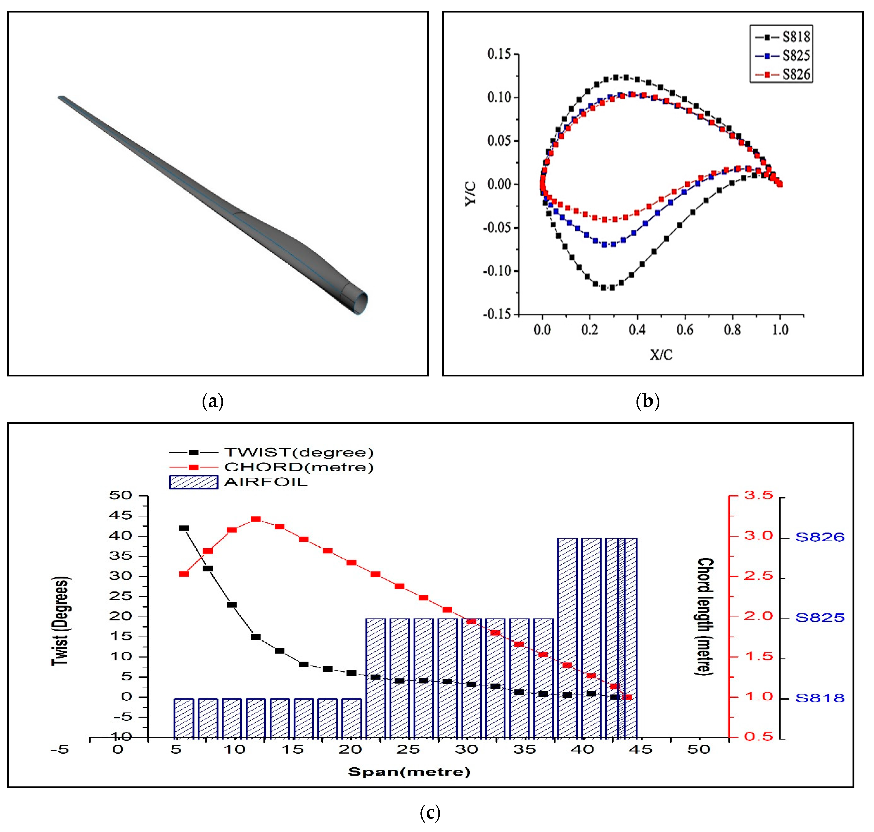
2.1.1. Design of Wind Turbine Model

The design of the wind turbine blade is accomplished by considering the geometric parameters and technical specifications given in the report [26]. The Solidworks [27] software has been used to design the three-dimensional blade. The blade is shown in Figure 1a. This blade uses three different types of an airfoil. Airfoils are kept along the span of the blade from root to tip. The airfoils used to build the blade of the wind turbine are shown in Figure 1b, and their properties are portrayed in the report [28].

Table 1. Main parameters of the wind turbine.

Parameters	Value	Unit
Rated power	1500	KW
No. of blades	3.0	Not Applicable
Rotor diameter	86.5	Metre
Rated wind speed	11.5	m/s
Rotational velocities	21.21	rpm
Pitch angle	0, 4, 8, 12, 16,	degree
Velocities	8, 9, 10, 11, 12, 16, 20, 24	m/s

provides the blade and rotor parameter specifications. To design a wind turbine rotor, its structural and aerodynamic specifications must be understood. From an aerodynamic point of view, choosing a thin airfoil is essential for better lifting. From a structural point of view, choosing a thick airfoil for high rigidity is the utmost vital criteria to avoid failure due to bending. Satisfying these two criteria is paramount in the design phase. Therefore, to meet both aerodynamic and structural specifications, specific airfoil must be mounted in a separate blade segment. This paper uses a thick airfoil at the root portion and positions a thin airfoil at the tip section. In this article, an additional one meter is taken to represent the blade connected to a hub, and the blade root is compensated 1 m from the rotation axis. This paper does not have the center. The distribution of chord, twist, and placement of airfoil is shown in Figure 1c.

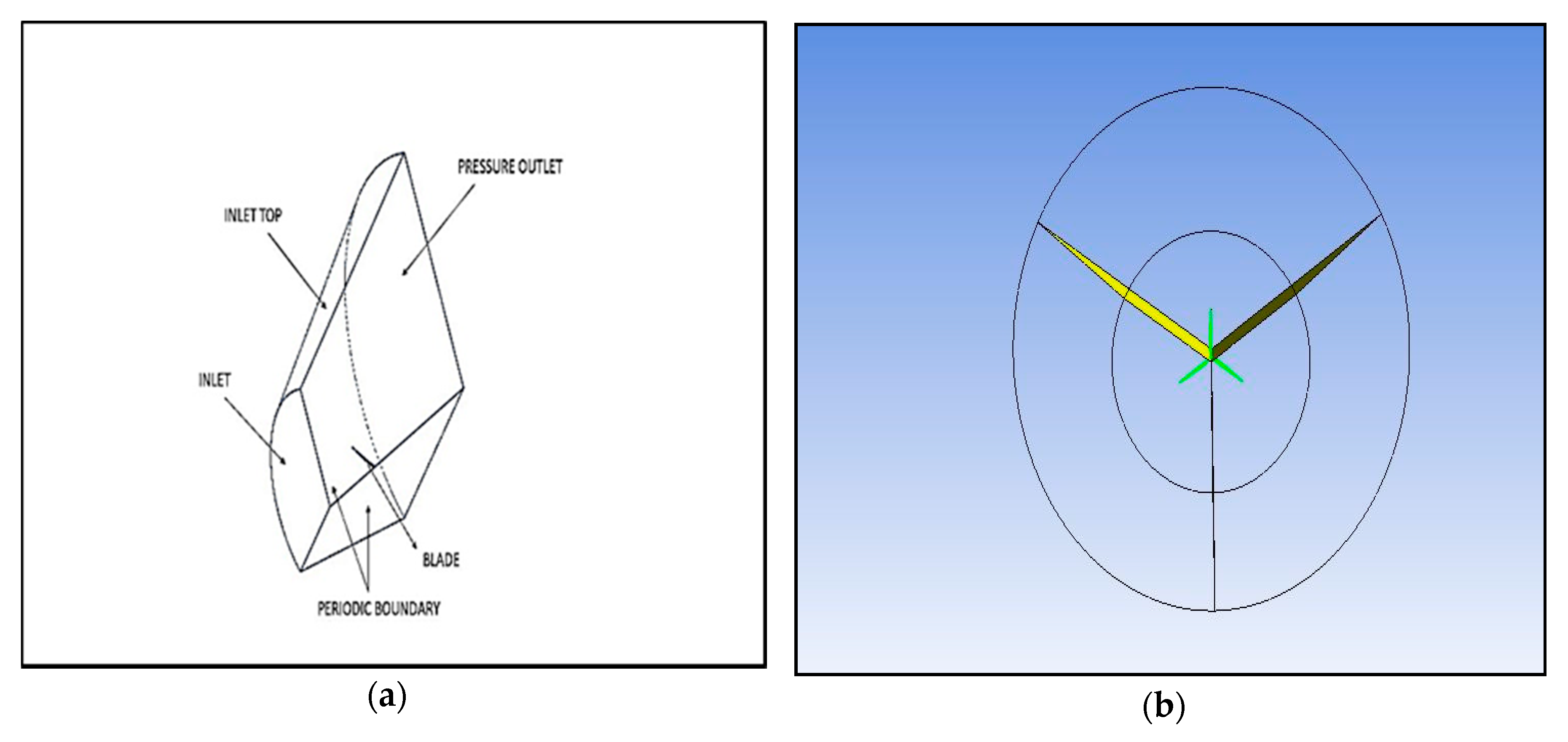
2.1.2. Computational Domain and Boundary Conditions

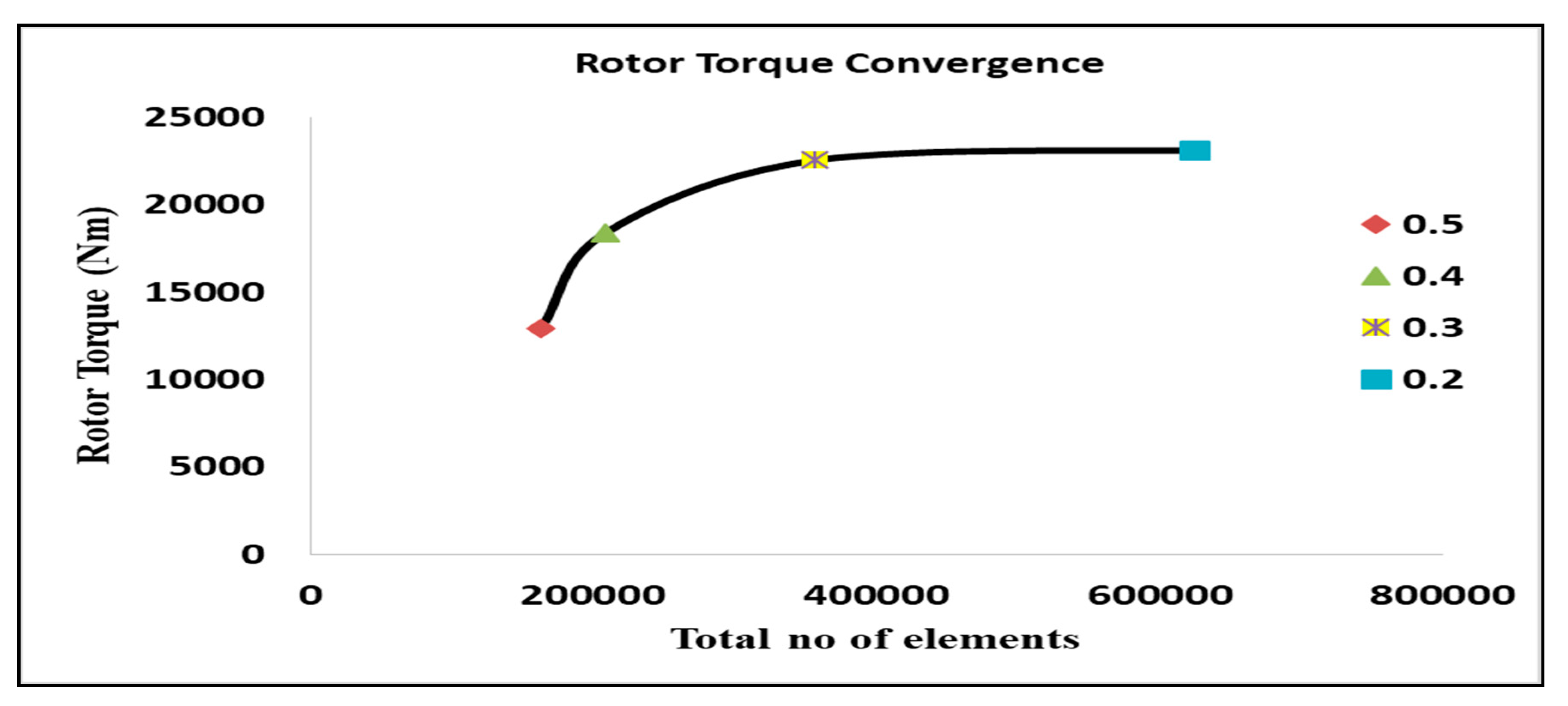
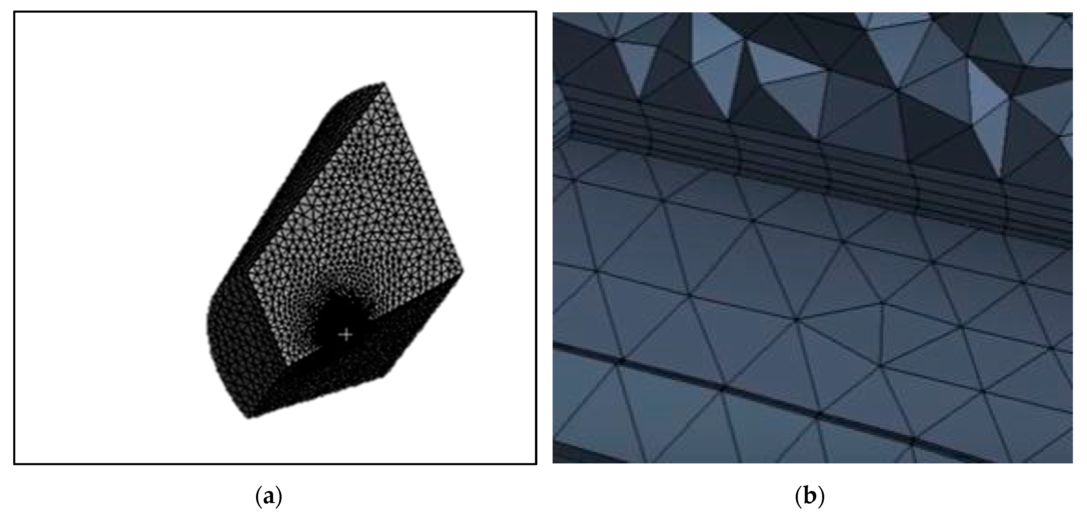
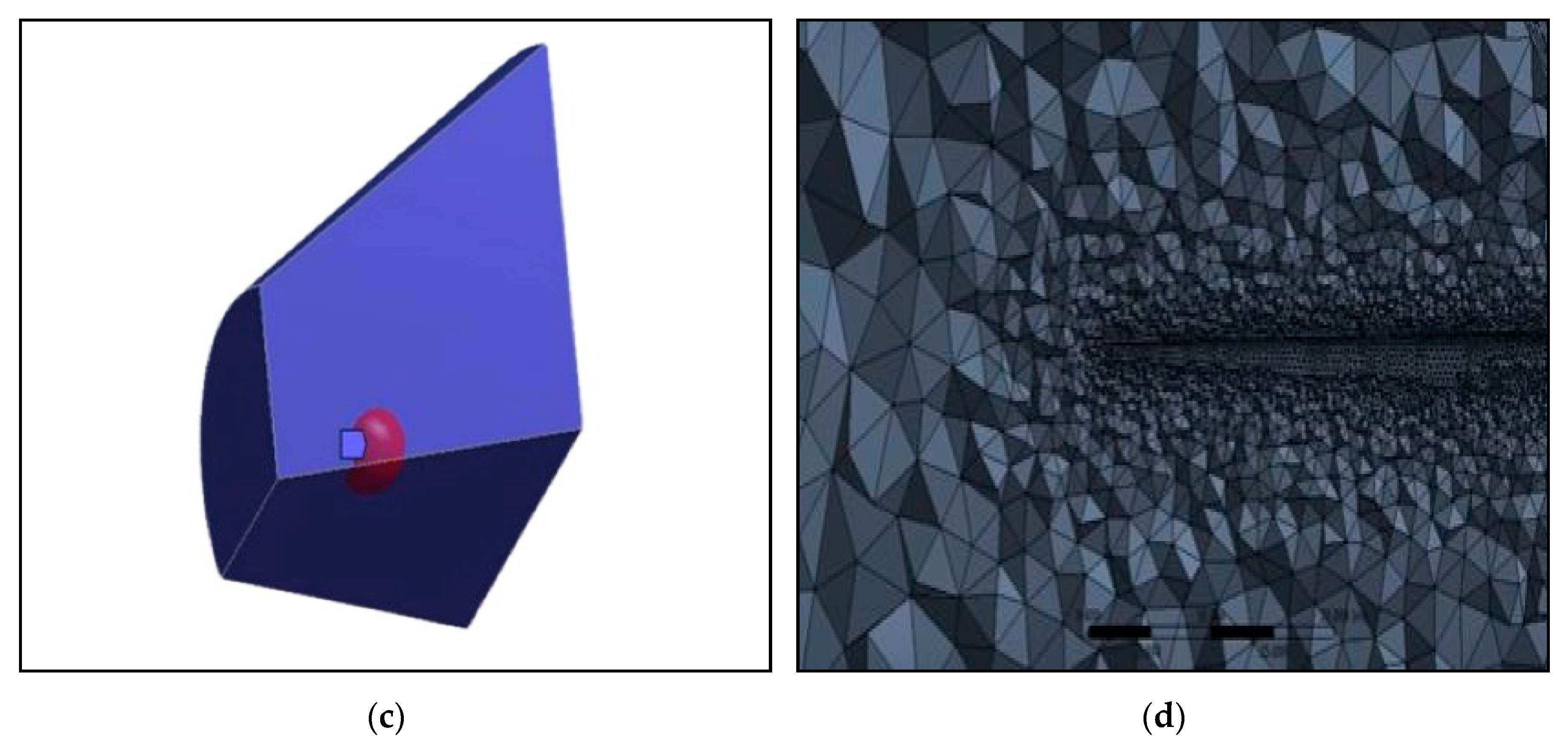
In this paper, the periodic boundary condition is implemented in the computational domain. To reduce the computational time, the domain is designed in such a way that it behaves symmetrically, and hence one-third of the full circle domain is designed [28,29,30]. One-third of the domain, along with boundary name and full circle domain, is shown in Figure 2a,b. Additional boundary conditions are highlighted in

Table 2. Boundary conditions.

Factors	Values
Side boundaries	Periodic boundary condition
Pressure outlet	1 atm
Turbulent intensity	5%
Turbulent viscosity	10

. The distance between the inlet and outlet portion of the domain is 270 m. While designing the domain, the global origin is kept at the center of the blade root. Here, the distance between the blade and the velocity inlet is 90 m, and the distance between the blade and pressure outlet is 180 m. The top portion of the domain is also given the same inlet velocity. Moreover, the arc radius at the velocity inlet and pressure outlet are taken as 120 and 240 degrees. Here, the domain resembles a conical shape to support the fact that the wake expansion trails the form of conical behind the turbine [31,32].

2.1.3. Meshing

A mesh sensitivity analysis is essential before determining the required mesh size. The mesh sensitivity analysis has been carried out in this study to determine the correct mesh size on the blade surface. The mesh size of 0.5, 0.4, 0.3, and 0.2 m was studied at the surface of the blade.

Table 3. Mesh sensitivity.

Parameter	Mesh Size at the Blade Surface
	0.5 m	0.4 m	0.3 m	0.2 m
Torque (Nm)	12,895	18,365	22,518	23,097
elements	163,217	208,431	356,628	624,099

shows the corresponding mesh dimension, complete no elements, and measured rotor torque. The rotor torque converges at a mesh size of 0.3 m, as seen in Figure 3 and Table 3. Additional adjustment of the mesh size to 0.2 m reflects a slight change, but the estimation time increases. Due to the time and precision of computation, the 0.3 mesh size is considered as an acceptable face size on the blade surface for CFD modeling in this analysis. In this paper, meshing starts with central mesh control and then with the local mesh handling. During the process of global meshing, tetrahedral cells are automatically configured for CFD and FLUENT. The advanced size feature adjusts to the proximity and curvature to render the curve with the appropriate form and skewness, with the relevance center retained at a medium level. In

Table 4. Nodes and elements for a different type of mesh.

Control Method	Type of Mesh	Sizing
Global mesh control	Tetrahedral	Advance size function
		Curvature (coarse)		Proximity (medium)
		nodes	elements	nodes	Elements
		32,736	185,999	60,778	34,3017
Local mesh control	hexahedral	Steps		nodes	element
		Match control		71,643	356,628
		Element size	0.3
		Inflation
		Sphere of influence
		Sphere radius	30 m
		Element size	2 m

, the number of nodes and elements obtained through the use of the globalized mesh and the local mesh control are shown. ANSYS FLUENT transforms the differential equations of the governing component into algebraic equations. The value (u, v, w, k, and ω) of the cell centers are derived from these algebraic equations. Here, u, v, and w display the velocity in x, y, and z-direction and k, and w represents the kinetic energy and the specific dissipation constant used to model turbulence. The paper uses grids based on a series of repeated elements composed of tetrahedral elements in 3D. Thus, the fluid domain is immediately formed as a tetrahedral, as seen in Figure 4a. Furthermore, the inflation layer is used to trap the boundary layer on an object, as shown in Figure 4b. To make it smoother across the circumference of the blade surface sphere of control, a radius of 30 m and the device size 2 m has been used, as seen in Figure 4c. Figure 4d demonstrates meshing near the surface of the blade.

2.1.4. Turbulence Modeling

The most complex form of fluid motion is the formation of turbulence. It is not only an unsteady flow but also has the potential to exert a three-dimensional nonlinear phenomenon. This turbulence, however, can be modeled by using the Navier-Strokes equations. In this paper, the k–ω shear stress transport (SST k–ω) model is applied to study the turbulence. This model combines two equations based on the k–ω model to represent two turbulence properties of the fluid flow. The first one is the turbulence kinetic energy (k), and the second is the specific dissipation rate (ω). This two-equation model developed by [33] has the benefit of being able to switch from the k−ε turbulence model [34], suited to simulating far-field flows, to a k−ω turbulence model [35], suited to modeling the boundary layer. This model has been used widely in the area involving wind turbine blades with well-disposed results [36,37]. However, to use this transport equation for the SST model to calculate the turbulent kinetic energy k and the specific dissipation rate ω, ANSYS FLUENT [25] is used to analyze turbulence modeling.

The Navier-Strokes formulation is described as:

$$\frac{\underset{\partial v}{\to }}{\partial t}+\left(\overrightarrow{V} \overrightarrow{\nabla }\right)\overrightarrow{V}=\overrightarrow{f}-\frac{1}{\rho }\nabla \rho +\vartheta \Delta \overrightarrow{V}$$

(1)

The two equations based on k–$\mathsf{\omega }$ are:

$$\frac{\partial }{\partial t}\left(\rho k\right)+\frac{\partial }{\partial x_i}\left(\rho k{u}_i\right)=\frac{\partial }{\partial x_j}\left({\mathsf{\Gamma }}_k\frac{\partial k}{\partial x_j}\right)+G_k-Y_k+S_k$$

(2)

$$\frac{\partial }{\partial t}\left(\rho \omega \right)+\frac{\partial }{\partial x_i}\left(\rho \omega u_i\right)=\frac{\partial }{\partial x_j}\left({\mathsf{\Gamma }}_w\frac{\partial w}{\partial x_j}\right)+G_w-Y_w+D_w+S_w$$

(3)

where $\vartheta$ = μρ is the coefficient of kinematic viscosity. In Equation (1), f is the distributed volume force. From Equations (2) and (3), G_k represents the generation of turbulence kinetic energy due to mean velocity gradients, and G_w represents the generation of ω. Whereas Γ_k, Γ_w represents the effective diffusivity of k and ω and Y_k, Y_w represents the dissipation of k and ω, D_w represents the cross-diffusion term, and S_w are user-defined source terms.

2.1.5. Solution Setup

In this paper, pressure velocity coupling is done by the coupled scheme. For getting pressure, the standard algorithm is used, and for evaluating the momentum equation, a second-order upwind algorithm is utilized. Moreover, to calculate the gradients, the least-squares cell-based algorithm is implemented. To get the turbulent kinetic energy and specific dissipation rate, the first-order upwind algorithm is used. The fluid is considered as air and is taken as incompressible [38]. The fluid density and viscosity of air are taken as 1.225 kg/m³ and 1.7894 × 103 kg/ms.

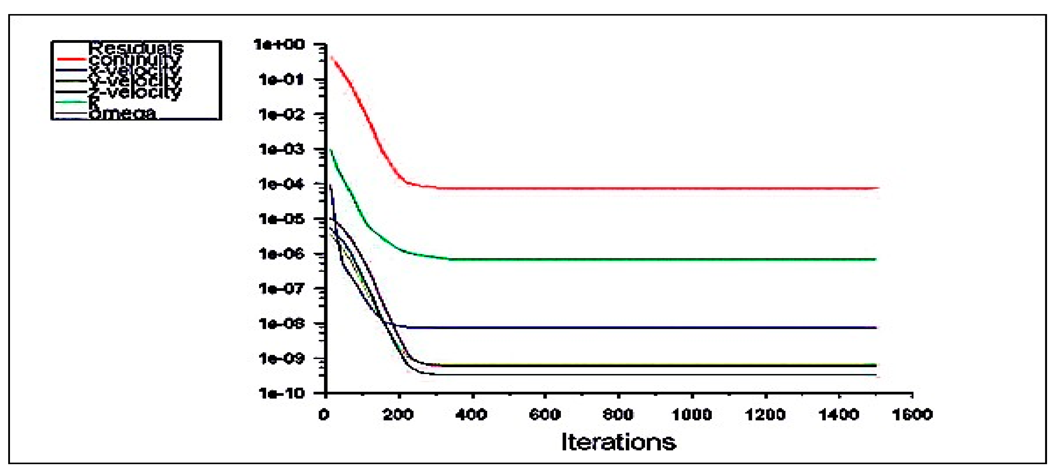
2.1.6. Residuals Convergence Criteria

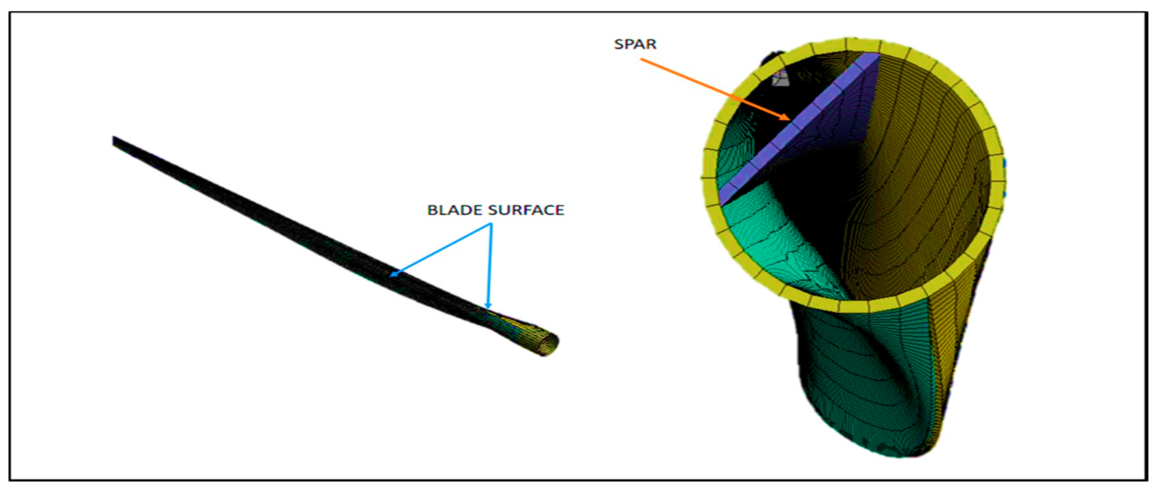
The residual plays an essential role in obtaining the convergence criteria of the CFD analysis. In this research, six variables of the residual values during the calculation process are monitored, and they are continuity, velocity in x, y, and z-direction, turbulent kinetic energy k, and specific dissipation rate ω. The solutions are considered to be converging if those residual values are below ${10}^{-4}$ [39], which is the typical value in wind turbine blade modeling for the residual convergence criterion. Figure 5 shows an example of residual values for wind speed 8 m/s, rotor speed 21.21 rpm, and a pitch angle of 4°. The solution convergence was determined by monitoring the residual history of cycle 1500 iterations.

2.2. FEA Modeling

The finite element analysis was conducted under the Ansys 15’s static structural framework. The blade considered here consists of a spar and blade surface. The thickness distribution of the spar and blade surface of the wind turbine blade is shown in Figure 6, and a three-dimensional blade configuration along with spar is shown in Figure 7. The blade shown in Figure 7 is composed of an outer surface and an inner spar. The thickness of the outside surface linearly decreases from 0.1 m at the root to 0.005 m at the tip shown in Figure 6a. The spar has a similar thickness behavior with 0.1 m at its closest point to the root and 0.03 m at the tip shown in Figure 6b.

To sum up, here are the thickness specifications needed along with their location concerning the global coordinate system (which represents the center of an imaginary hub and thus the center of rotation). These thicknesses are very close to the real turbine. The materials [40,41] that are allocated to the blade for structural analysis in this paper possess numerous auxiliary properties that sustain the structure. The standpoint of such materials is the ability for a strong stiffness to weight ratio. Four materials are used in this analysis for structural analysis, and their mechanical properties, such as elastic modulus, and density, are shown in

Table 5. Material properties.

Material Name	Elastic Modulus [GPa]	Density [Kg/m3]
Kevlar	179	1470
Technora	70	1390
Glass-S	88	2540
Swancor-2511A	19.2	1859

.

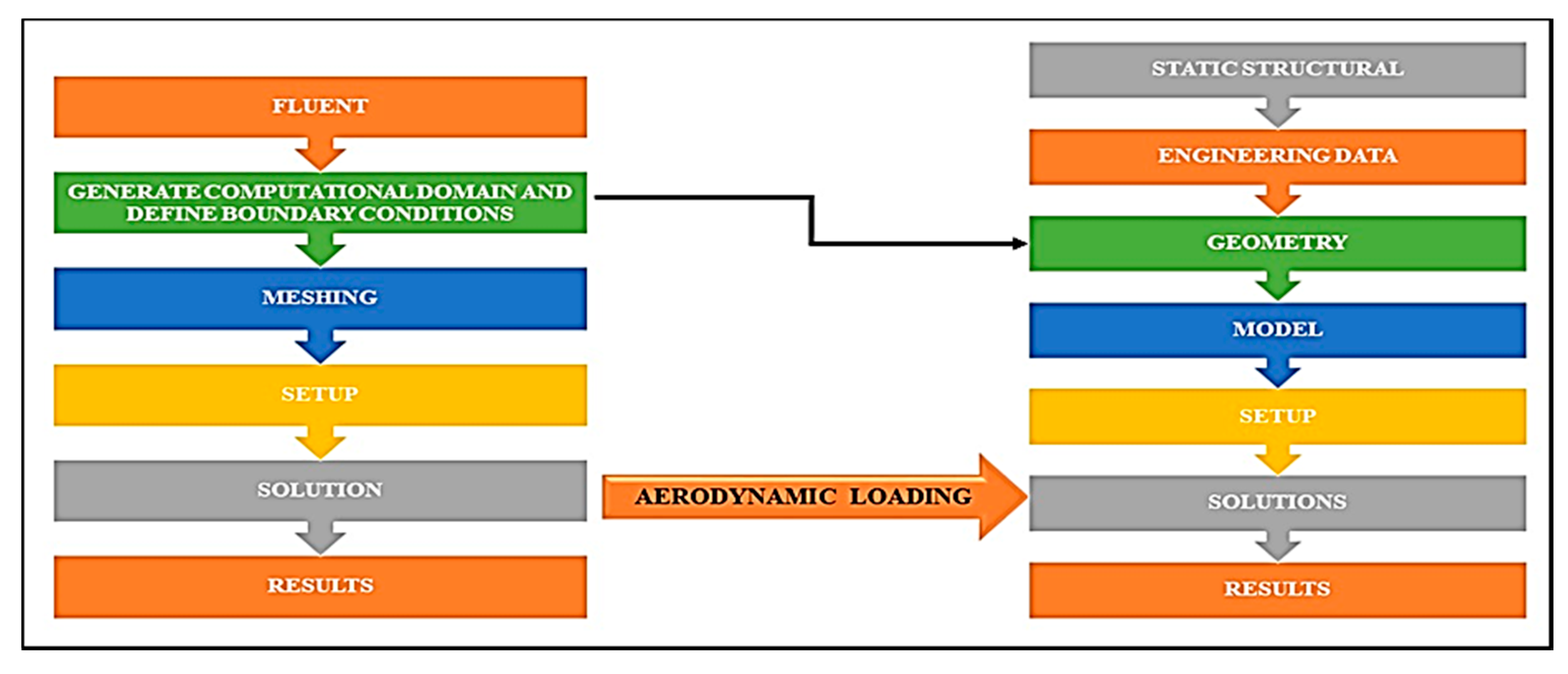
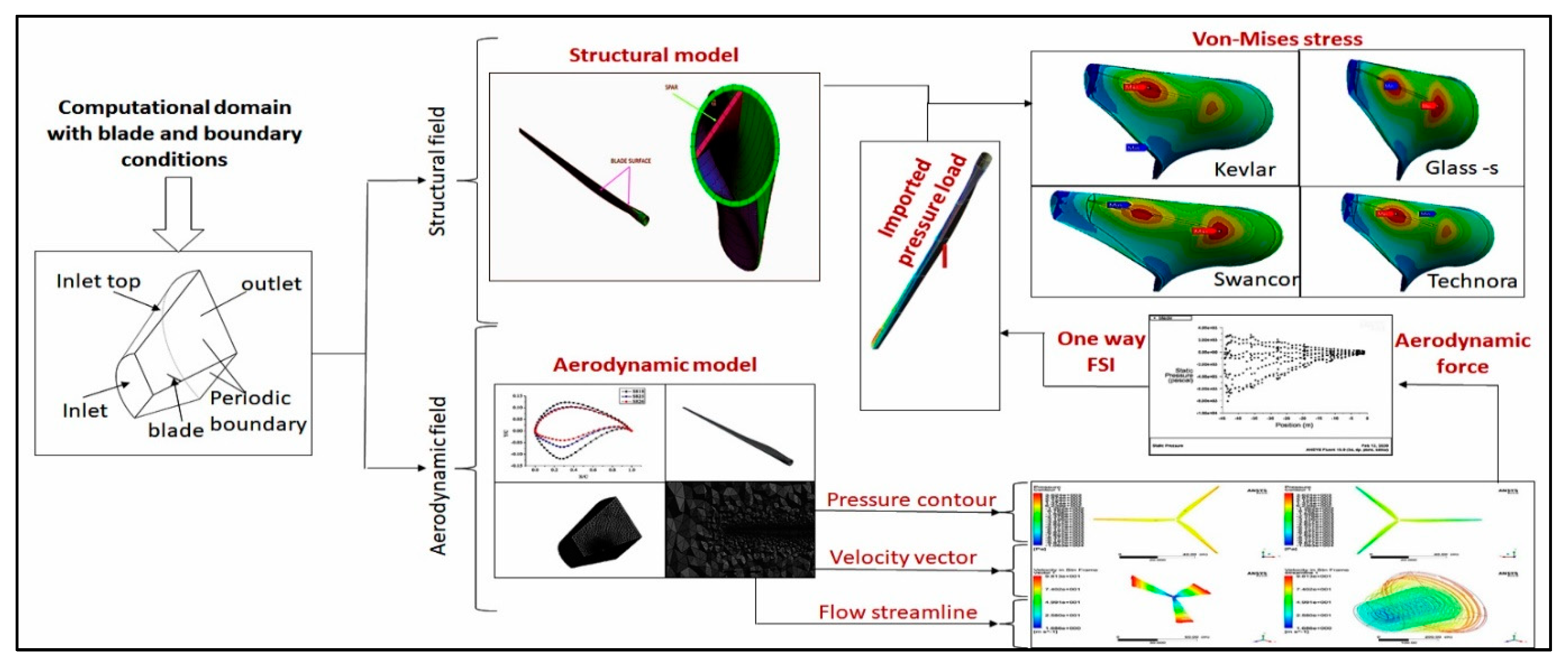
2.3. One-way FSI Coupling

Fluid-structure interaction (FSI) is an interaction between the flexible structure and the fluid flow stream. In this article, wind turbine execution is a result of the contact between the aerodynamics of wind current and the structural model. ANSYS software is used to conduct FSI investigations. For fluid and structure, two computational zones were regarded, which are separately investigated according to their mesh and significant equations. The schematic diagram of one-way FSI is shown in Figure 8, and the complete layout of aerodynamic and structural coupling is shown in Figure 9.

3. Results and Discussion

In this section, results from ANSYS simulations are manifested. Here a detailed analysis of the 3D simulation of the blade is manifested. The complete simulation has been accomplished by considering the 120° sector of the turbine rotor.

3.1. Three-Dimensional Simulations

Wind-turbine blades are intended for generating power by harnessing kinetic energy through rotational effect, in which blades have a variation in thickness from root to tip, allowing the blade to withstand higher stress and moment close to the root than that towards the tip. Similarly, a twist to the blade is given along the span of the blade to get the maximum power coefficient. Presently, the optimization of the geometric parameters works productively in operational conditions when the turbine is rotating. However, when the turbine is not rotating, particularly in a situation when the yaw and pitch control mechanism is disconnected or during a turbine-erection stage, the optimized blade twist will make the stream 3D misleadingly contrasted with the genuine rotor stream itself. Subsequently, during the shutdown, without a wind turbine control system, the α (angle of incidence) of the flow on the blade is dictated by the free wind direction, and the wind turbine may work outside the restricted operational range. In such stationary circumstances, complex 3D impacts may exist attributable to both the working conditions and the 3D complex turbine geometry. Thus, the performance of 2D simulation is sufficiently bad to comprehend flow dynamics in such conditions. It presently features the significance of performing stationary simulations, which can represent the effect of bluffness of the turbine geometry and evolving cross-segment on optimal design parameters and flow physics. Therefore, this section provides the results of 3D simulation by considering a stationary three-dimensional wind turbine blade for analysis.

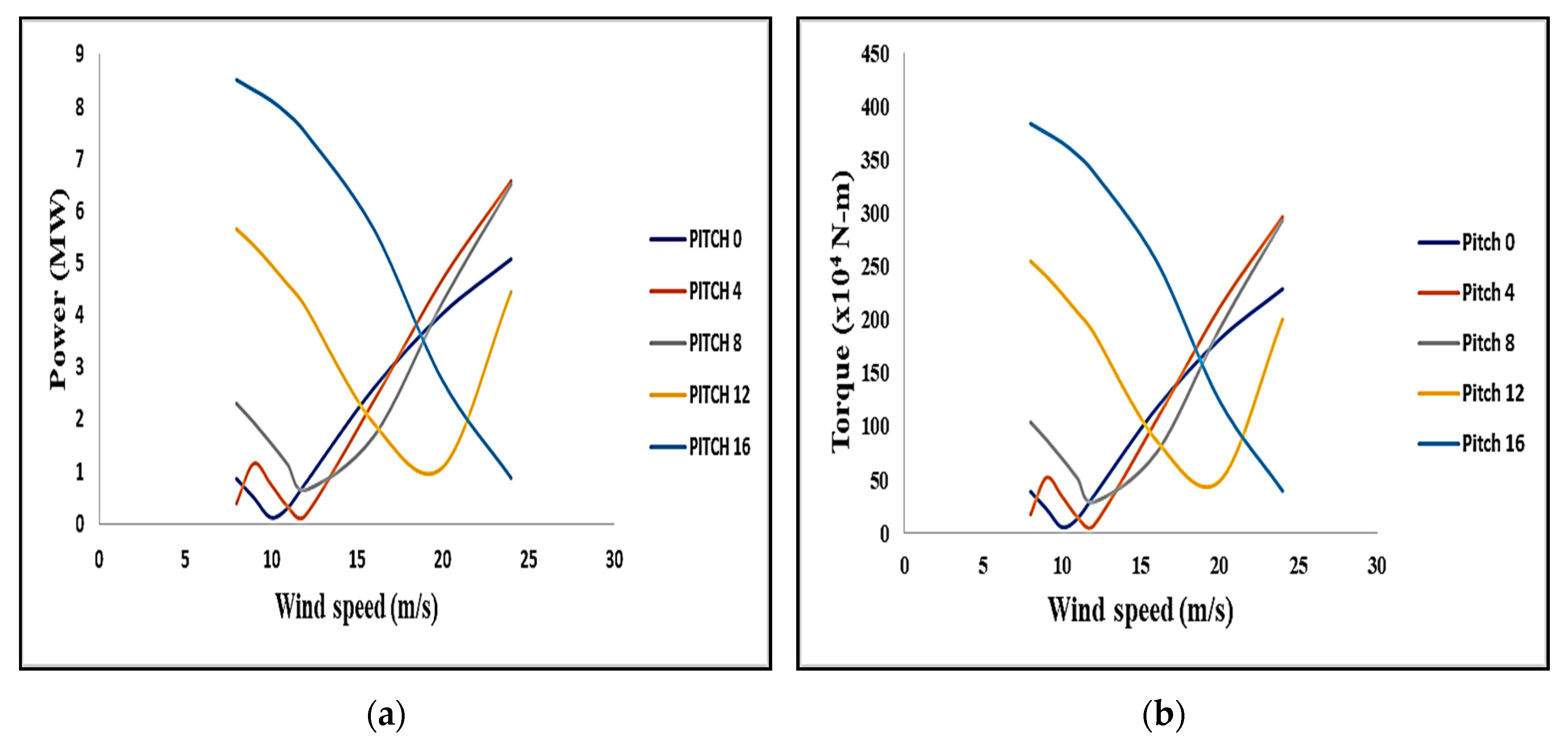
3.1.1. Estimation of Torque and Power

Figure 10a,b highlights the effect of pitch angles on performance parameters such as torque and power. Each parameter has its degree of significance in determining wind turbine reliability. Due to the wind turbine physics, for a given wind speed, there is maximum power and maximum torque that comes out when the blade pitch angle is set at a specific value, and free stream velocity strikes the span of the blade at a certain angle. Hence, in this study, five-pitch angles of 0, 4, 8, 12, and 16° have been considered to decide the wind speed at which the power output of the wind turbine reaches its greatest. While conducting the numerical analysis of wind turbines, torque is considered as an important parameter in determining the power of the wind turbine blade. Figure 10 gives an idea that the pitch angle has some impactful presence in getting the torque and power ascertaining wind turbine efficiency for free stream velocity. Thus, it becomes important to see the impact of the pitch angle on the performance parameter of the wind turbine blade. In Figure 10a, the variation of torque with different wind speeds at different pitch angles has been illustrated, which says that for a pitch angle of 0°, the torque decreases when the velocity changes from 8 to 9 m/s, but after 9 m/s the torque monotonically increases until 24 m/s. However, when the blade is given a pitch angle of 4°, the torque increases for the first two velocities that are 8 and 9 m/s, then shows some decrease pattern until 12 m/s in a step of 1 m/s, but, after 12 m/s the torque shows some increment and continues until 24 m/s. Now, for a pitch angle of 8°, the torque starts to increase after 16 m/s, and for a pitch angle of 12°, the torque starts to increase after 20 m/s. It is interesting to note that for a pitch angle of 16°, the torque consistently decreases with an increase in the wind speed. The trend of the power curve given in Figure 10b is the same as the trend shown in Figure 10a. Hence, after getting the torque value from the CFD simulation, the generated power can be easily determined using Equation (4):

P = T × ω

(4)

where P is power (MW), T is torque (N-m), and $\mathsf{\omega }$ is the angular velocity (rad/s).

3.1.2. Verifications

The verification of the numerical investigation is accomplished by comparing it with an empirical equation and is shown in

Table 6. Comparison of tangential velocity.

Pitch (Degree)	V (m/s)	Tangential Velocity
		Numerical	Analytical	Error (%)
8°	12	98	96.015	2.067

,

Table 7. Comparison of radial force for Kevlar and Technora material.

		Material	Radial Force (N)		Material	Radial Force (N)
		Kevlar			Technora
Pitch (Degree)	V (m/s)	Numerical	Analytical	Error (%)	Numerical	Analytical	Error (%)
8°	12	1.50 × 106	1,473,265.61	1.92323677	1.42 × 106	1,418,564	0.101206

and

Table 8. Comparison of radial force for Swancor-2511 A and Glass-S material.

		Material	Radial Force (N)		Material	Radial Force (N)
		Swancor-2511 A			Glass-S
Pitch (Degree)	V (m/s)	Numerical	Analytical	Error (%)	Numerical	Analytical	Error (%)
8°	12	1.89 × 106	1,888,030.386	0.088431517	2.59 × 106	2,592,159.361	0.059435

. The equation used for the comparison is given in Equations (5) and (6). Figure 11a,b indicates the direction of the tangential velocity and force reaction.

Tangential velocity = r × ω

(5)

Root radial force = m × r × ω²

(6)

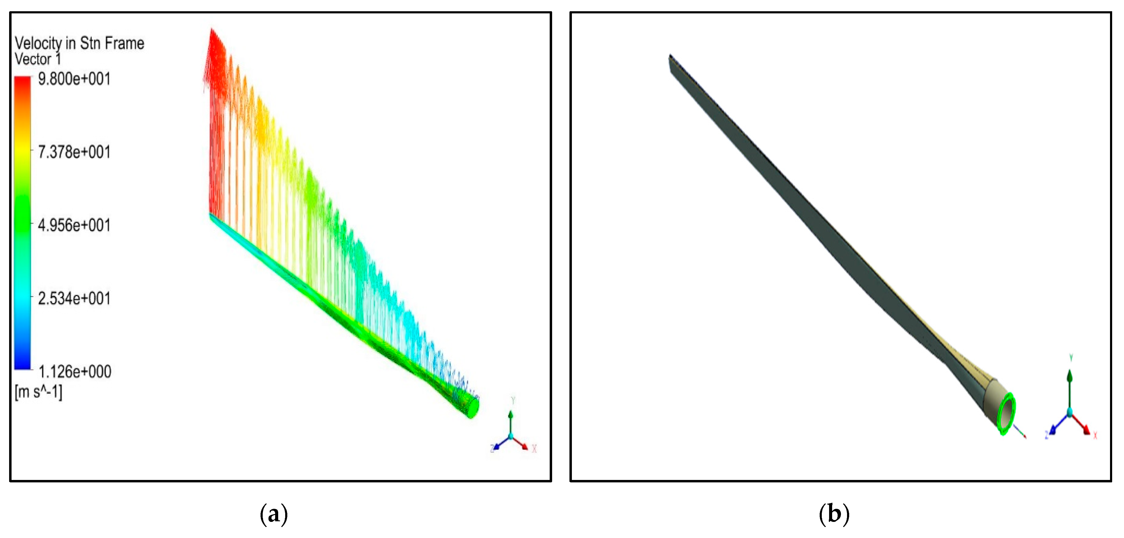
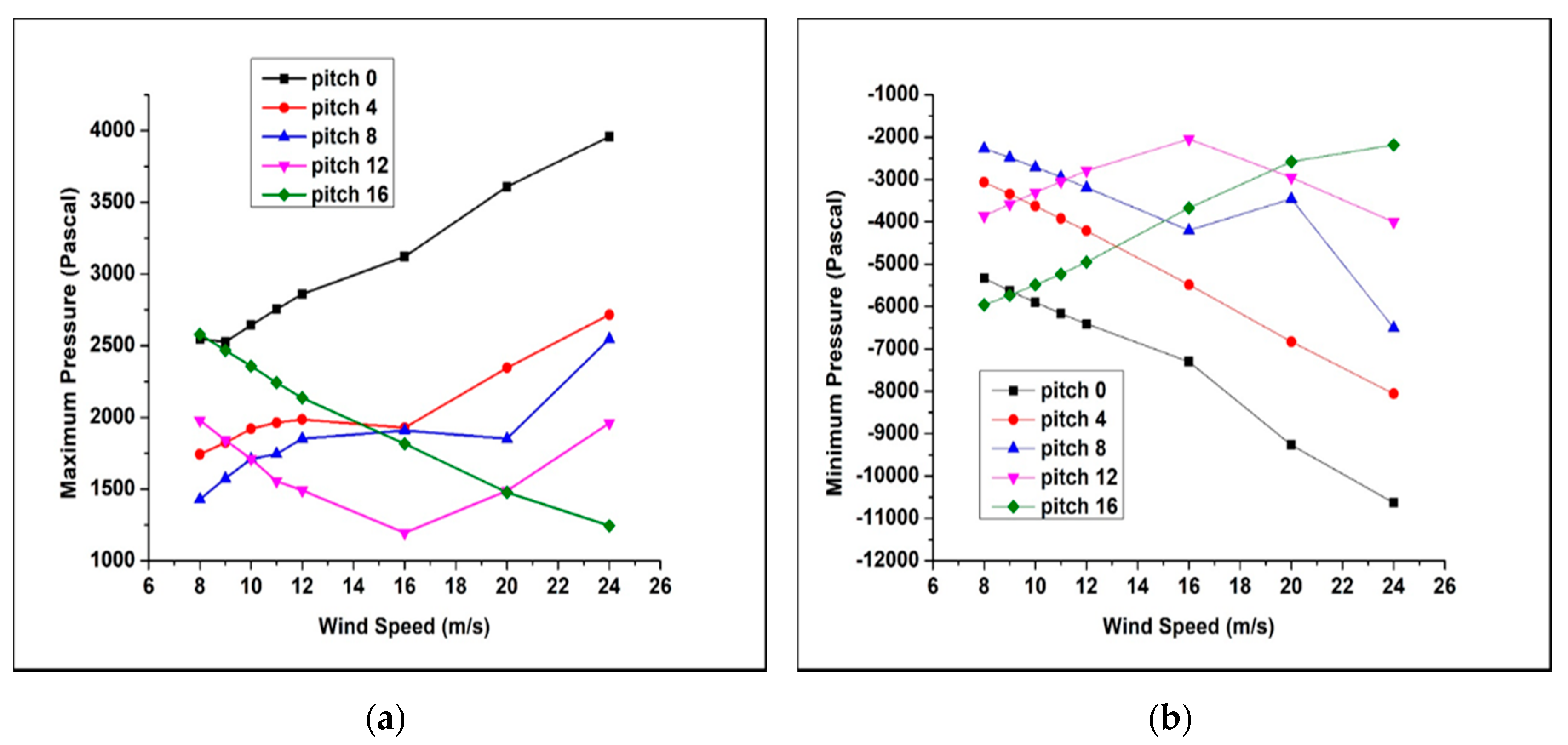
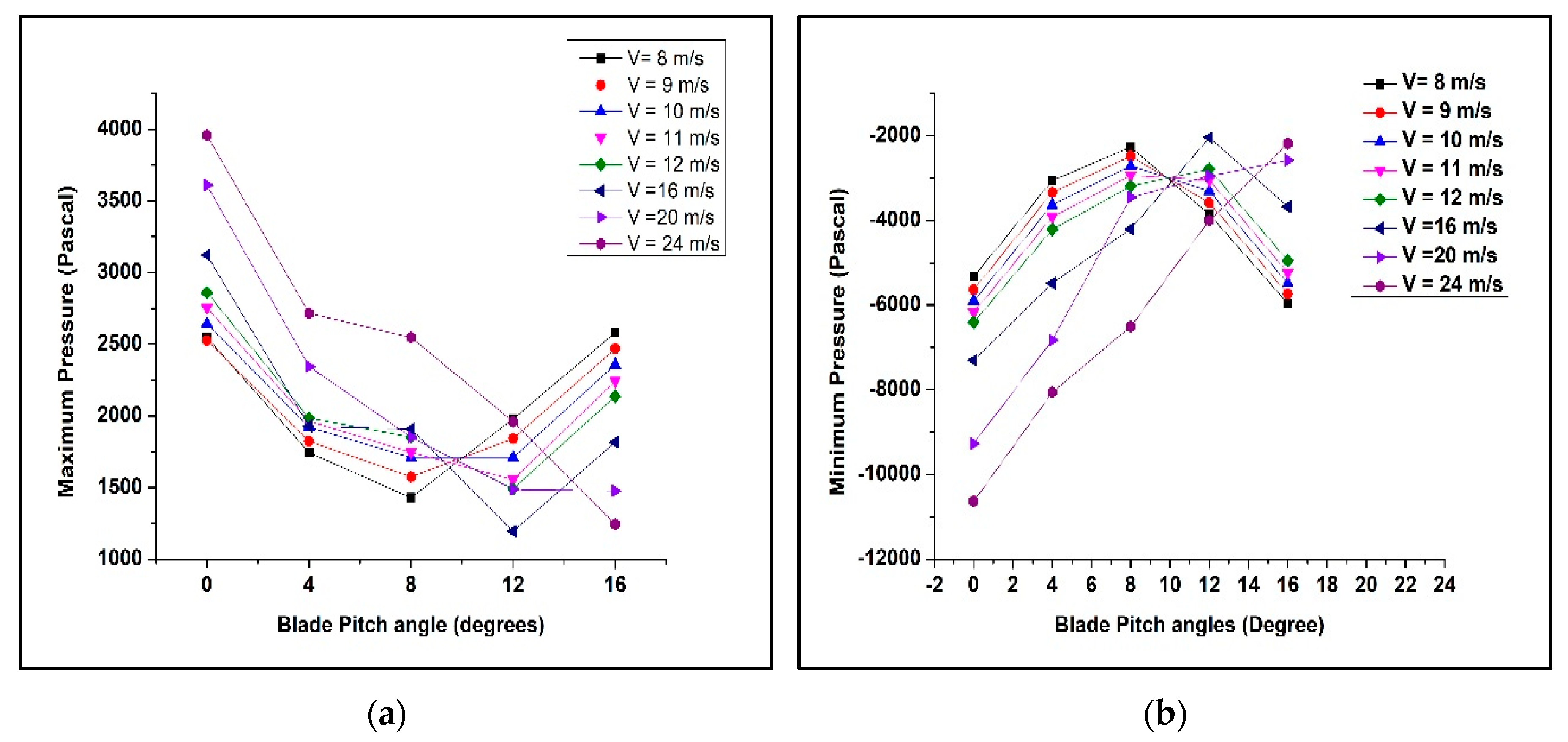
3.1.3. Pressure Distributions

The graph shown in Figure 12 and Figure 13 reveals the pressure distribution of the blade for different pitch angles and wind speed. Here, the pressure side of the blade is indicated as the windward side and is highly subjected to maximum pressure and suction one as the leeward side, which shows a negative pressure. Initially, the fluid reaches the leading edge of the blade, and for this purpose, a more significant variance exists primarily at the tip and contributes to the fluctuation of pressure. Here, the rotational effect is the reason behind the pressure distribution, which consequently generates the lift. However, as the blade is pitched, the blade becomes more collinear with the flow direction, which further shifted the stagnation point on to the leeward side and resulted in a decrease in negative pressure when the velocity is low. In this section, the distribution of pressure is stated by considering the three-stall regions. One is a pre-stall region that occurs before 10 m/s; the second is the dynamic stall region that comes into play when the wind speed is higher than 10 m/s, and the third is the deep stall region, which occurs at a velocity more than 20 m/s. As can be seen from Figure 12 and Figure 13, in the pre-stall region (8, 9, and 10 m/s), the pressure distribution shows some significant change as the pitch angle of the blade changes. In Figure 12a and Figure 13a, it is observed that when the velocity is 8 m/s, the trend of maximum pressure decreases exponentially from 2548 Pascal at 0° pitch angle to 1430 Pascal at 8° pitch angle. However, it increases again to 1979 Pascal at 12° pitch angle and 2579 Pascal at 16° pitch angle. Now, one can say from this trend that when the velocity is 8 m/s and an 8° pitch angle is taken for analysis, the blade will face less positive pressure and eventually less impact on the blade structure. The same trend is being followed when the velocity is 9 m/s where the maximum pressure decreases from 2526 Pascal at a 0° pitch angle to 1574 Pascal at an 8° pitch angle and then increases to 1841 Pascal at a 12° pitch angle and 2468 Pascal at a 16° pitch angle. Therefore, in the pre-stall region, the 8° pitch angle becomes a pivot angle, which, when taken for analysis, delivers less maximum pressure. However, when a velocity of 10 m/s is considered, the value of maximum pressure decreases up to a 12° pitch angle and then shows sudden increment; this is due to the onset of dynamic stall. Now, for the dynamic stall region, velocity such as 11, 12, and 16 m/s have been considered in this study. Now, when this velocity was taken, and different pitch angles were implemented in the analysis, the trend is such that the pressure decreases until a 12° pitch angle and then increases for a 16° pitch angle. Now, for Figure 12b and Figure 13b, the trend of minimum pressure distribution is such that as the velocity of the flow increases, the negative pressure also increases but for pitch angle of 0, 4, and 8°. However, it is observed that for a pitch angle of 8°, there is a slight decrease in the negative pressure when the velocity changes from 16 to 20 m/s, and for pitch angle of 12 and 16°, the negative pressure decreases monotonically.

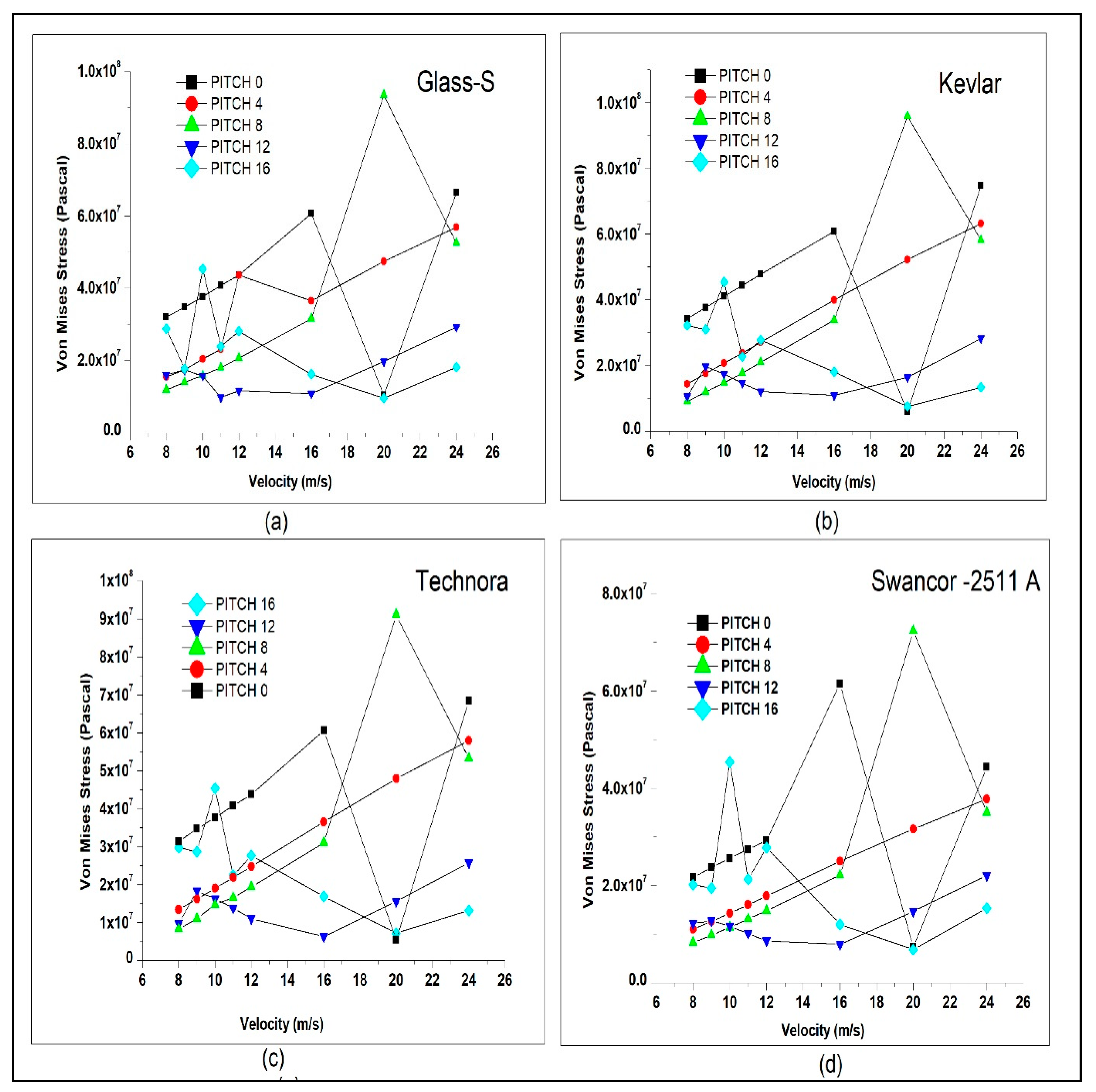
3.1.4. Deformation and Von-Mises Stress

In this study, four materials have been chosen to carry out the stress analysis on the blade. The material specification is given in Table 5. Moreover, in this section, the effect of pitch on the blade by using different materials has been studied by implementing deformation and Von-Mises stress analysis. As can be seen from Figure 14a–d, when an 8° pitch angle is considered, it is found that maximum stress is observed at 20 m/s irrespective of the material used in the wind turbine blade. The curve, which possesses an 8° pitch angle is varying in such a way that Von-Mises stress shows an increase in value until 20 m/s and then suddenly decreases when the velocity of 24 m/s is considered. In addition, Figure 14a–d also gives an idea that there is a significant increase and decrease in the Von-Mises stress when the velocity progresses. As different materials have been used, the below curves shown in Figure 14a–d is demarcated based on the material assigned to the blade. It is such that when a velocity of 8 to 12 m/s is considered, the percentage increase in the Von-Mises stress is observed. The percentage increase was between 13% to 16% for Glass-S material, 18.6% to 32.6% for Kevlar material, 16.9% to 33.7% for Technora material, and 13.4% to 18.8% for Swancor-2511 A. In addition; there is an increase of 52.2% for Glass-S material, 60.8% for Kevlar material, 60.3% for Technora material, and 48.8% for Swancor-2511A that are observed in the value of Von-Mises stress when velocity changes from 12 to 16 m/s. Moreover, moving from 16 to 20 m/s, a slight increase in Von-Mises stress can be analyzed in Figure 14a–d. Now, as velocity approaches 24 from 20 m/s, there is a percentage decrease of Von-Mises stress that occurs, and it is such that when the Glass-S material is used, there is a decrement of 43.8%. For material Kevlar, it is found that a 39.4% decrement occurred. However, Technora and Swancor-2511 show a percentage decrease of 41.5% and 51.7%, respectively. It is interesting to note that irrespective of the different materials used, a minimum value is observed at a pitch angle of 12° when the velocity varies from 11 to 16 m/s, which makes this pitch more convenient for dynamic stall conditions. However, it is to be noted that for a pitch angle of 12°, when the Glass-S material is used, there is a slight increment in the Von-Mises stress when velocity changes from 11 to 12 m/s, which for different materials show the decreasing pattern. Now, for a pitch angle of 0°, two peak points indicate the maximum Von-Mises stress as compared to others, which take place at velocity 16 and 24 m/s, and between these two velocities, 24 m/s shows a higher value of stress. However, the minimum pitch value of Von-Mises stress occurred at 20 m/s. Unlike a pitch angle of 0°, a 4° angle pitch shows two peak points only for the Glass-S material, and it occurs when the velocity is 12 and 24 m/s. However, it is interesting to note here that also the maximum Von-Mises stress comes at 24 m/s, but the minimum stress is observed at 8 m/s. Also, irrespective of different wind speeds, it has been found that for a pitch angle of 4°, all materials possess the increasing trend of Von-Mises stress variation. However, discontinuity in the curve is observed for the Glass-s material when the velocity changes from 11 to 16 m/s. As mentioned above, for every other pitch, some changes occurred, which gives an idea that wind turbines can also be operated by controlling the pitch. From the above explanation, it has been found that the maximum Von-Mises stress occurred at 24 m/s when the pitch angles of 0°, 4°, and 12° are taken for the analysis. However, when a pitch angle of 8° and 16° is considered, there comes some discontinuity in the curve, and maximum stress occurred at 20 m/s and 10 m/s. Apart from this, in Figure 14a–d, unlike the two peak points observed above, a pitch angle of 16° reflects three peak points of Von-Mises stress, and it takes place when the velocity is 10, 12, and 24 m/s. Now, for the blade deformation, complete numerical results for every respective pitch are shown in

Table 9. Deformation of the blade for a zero-degree pitch angle at different wind speeds.

Velocity (m/s)	Glass-S (m)	Kevlar (m)	Technora (m)	Swancor-2511 A (m)
8	0.55123	0.29617	0.70182	1.7665
9	0.61139	0.33111	0.78548	1.9949
10	0.67586	0.36432	0.86468	2.1908
11	0.73686	0.39832	0.94582	3.3891
12	0.79715	0.43714	1.0252	2.5813
16	1.1564	0.56919	1.4525	5.1838
20	0.050511	0.016281	0.036135	0.12669
24	1.2694	0.69886	1.6568	4.1439

through Table 13. The blade sums up to absolute deformation under the given operating conditions. Blade deformation usually occurs at the tip and is almost negligible close to the center. It is due to the rotation and the speed of the airflow, which gives high loads to the tip. Researchers have shown that the maximum deformation should lie well below 3.3 m to avoid the blade coming in contact with the tower [29]. In Table 9,

Table 10. Deformation of the blade for a pitch angle of 4° at different wind speeds.

Velocity (m/s)	Glass-S (m)	Kevlar (m)	Technora (m)	Swancor-2511 A (m)
8	0.22622	0.11255	0.26859	0.70576
9	0.26927	0.14384	0.34039	0.8738
10	0.3363	0.17497	0.41434	1.0701
11	0.39292	0.20617	0.48803	1.2587
12	0.45096	0.23819	0.56308	1.4486
16	0.67612	0.3682	0.87393	2.2185
20	0.90612	0.49018	1.1666	2.9492
24	1.0938	0.5971	1.4175	3.5604

,

Table 11. Deformation of the blade for a pitch angle of 8° at different wind speeds.

Velocity (m/s)	Glass-S (m)	Kevlar (m)	Technora (m)	Swancor-2511 A (m)
8	0.13246	0.060564	0.14079	0.39237
9	0.18135	1.19 ×107	0.21102	0.56543
10	0.23053	0.11691	0.27955	0.73666
11	0.27816	0.14886	0.3526	0.90654
12	0.3461	0.17977	0.42606	1.1046
16	0.57654	0.30864	0.73251	1.876
20	1.6784	0.92248	2.1815	5.4573
24	1.008	0.54747	1.301	3.2951

,

Table 12. Deformation of the blade for a pitch angle of 12° at different wind speeds.

Velocity (m/s)	Glass-S (m)	Kevlar (m)	Technora (m)	Swancor-2511 A (m)
8	0.05974	0.061052	0.13894	0.23501
9	0.26174	0.16522	0.39661	0.9515
10	0.22748	0.14308	0.3439	0.83118
11	0.52217	0.11596	0.2827	0.6858
12	0.14146	0.090755	0.21136	0.52744
16	0.061012	0.032496	0.047455	0.15458
20	0.27501	0.14175	0.34118	0.89583
24	0.51484	0.27271	0.64256	1.6647

and

Table 13. Deformation of the blade for a pitch angle of 16° at different wind speeds.

Velocity (m/s)	Glass-S (m)	Kevlar (m)	Technora (m)	Swancor-2511 A (m)
8	0.49259	0.28613	0.68602	1.7075
9	1.4003	0.27395	0.65709	1.636
10	0.89309	0.4395	1.1227	4.0426
11	0.043996	0.21269	0.53191	1.7097
12	0.45884	0.23969	0.61567	2.1882
16	0.22886	0.1448	0.34868	0.84425
20	0.039418	0.034896	0.086884	0.19509
24	0.21318	0.0905	0.22869	0.89097

, it has been found that when materials such as Kevlar, Glass-S, and Technora are considered, the blade reflects deformation which is below 3.3 m, but when a material such as Swancor-2511 A is taken into account blade deformation, it exceeds the limit for every pitch angle except a pitch angle of 12°. The worst deformation can be seen when the pitch angle is 0° for 16 m/s, 16° for 10 m/s, and 8° for 20 m/s.

4. Conclusions

In this study, the effect of blade pitch angle on the aerodynamic and structural characteristics of the HAWT was investigated via the fluid-structure interaction (FSI) coupling, and the conclusions can be summarized as follows:

• A pitch angle of 16° is not suitable for the analysis and for the experimental purpose as it shows a decrease in the power value for wind speed.
• A pitch angle of 0°, 4°, and 8° has shown a better power outcome as compared to other pitches.
• The torque acting on the blade is maximum when a pitch angle of 4° and 8° is considered for the analysis.
• For every pitch angle and wind speed, a maximum deformation of the blade obtained for Kevlar, Technora, and Glass-s comes to be lower than the clearance of the tower (3.3 m), suggesting that, under all operating conditions, the blade cannot hit the tower.
• The maximum equivalent stress (Von-Mises stress) for Kevlar, Glass-S, and Glass-E are found to be well suited to the design limit.
• It is observed that for a pitch angle of 0°, velocity 11 m/s, pitch angle of 8°, velocity 20 m/s, pitch angle of 4°, velocity 24 m/s, and pitch angle of 10°, and velocity 10 m/s blade deformation exceeds the tower clearance when the Swancor-2511 A material is considered.
• The finding of the current study supports improvement of the aerodynamic performance of a horizontal axis wind turbine in the following ways:
• Optimization of the wind turbine blade is conceivable by detecting the best pitch angle.
• It is possible to boost the mean electrical power significance by outfitting wind turbines with section pitch angles distributions.
• Identifying best pitch angles can help in developing a control strategy to reduce loads fluctuation and regulate the power output.
• The results from the numerical simulation can help in developing a small wind turbine with various pitch angles, which can be tested inside a low-speed wind tunnel. This experiment can help in verifying the feasibility and efficiency of the turbine. The experimental results can be excellent benchmark data for the computational and theoretical modelers to validate their models before undertaking simulations of more realistic conditions both in terms of turbine support and geometry.
• This article can help the researcher derive an optimal blade pitch function based on the best pitch angle, which can further help in designing the blade pitch control device.
• From this study, one can identify the desirable pitch angle and can reduce the strength of the unsteady load caused by the wave current action without too much loss of power.

References

1. Global Wind Report 2018. Global Wind Energy Council. 11 October 2019. Available online: https://gwec.net/global-wind-report-2018/ (accessed on 25 March 2020).
2. Dai, J.; Yang, X.; Wen, L. Development of wind power industry in China: A comprehensive assessment. Renew. Sustain. Energy Rev. 2018, 97, 156–164. [Google Scholar] [CrossRef]
3. Premalatha, M.; Abbasi, T.; Abbasi, S.A. Wind energy: Increasing deployment, rising environmental concerns. Renew. Sustain. Energy Rev. 2014, 31, 270–288. [Google Scholar]
4. Wang, L. Nonlinear Aeroelastic Modelling of Large Wind Turbine Composite Blades. Ph.D. Thesis, University of Central Lancashire, Preston, UK, 2015. [Google Scholar]
5. Makridis, A.; Chick, J. Validation of a CFD model of wind turbine wakes with terrain effects. J. Wind Eng. Ind. Aerodyn. 2013, 123, 12–29. [Google Scholar] [CrossRef]
6. Orlandi, A.; Collu, M.; Zanforlin, S.; Shires, A. 3D URANS analysis of a vertical axis wind turbine in skewed flows. J. Wind Eng. Ind. Aerodyn. 2015, 147, 77–84. [Google Scholar] [CrossRef] [Green Version]
7. Plaza, B.; Bardera, R.; Visiedo, S. Comparison of BEM and CFD results for MEXICO rotor aerodynamics. J. Wind Eng. Ind. Aerodyn. 2015, 145, 115–122. [Google Scholar] [CrossRef]
8. Tu, J.; Yeoh, G.H.; Liu, C. Computational Fluid Dynamics: A Practical Approach; Butterworth-Heinemann: Oxford, UK, 2018. [Google Scholar]
9. Hansen, M.O.L.; Sørensen, J.N.; Voutsinas, S.; Sørensen, N.; Madsen, H.A. State of the art in wind turbine aerodynamics and aeroelasticity. Prog. Aerosp. Sci. 2006, 42, 285–330. [Google Scholar] [CrossRef]
10. Zhang, P.; Huang, S. Review of aeroelasticity for wind turbine: Current status, research focus and future perspectives. Front. Energy 2011, 5, 419–434. [Google Scholar] [CrossRef]
11. Wang, L.; Liu, X.; Renevier, N.; Stables, M.; Hall, G.M. Nonlinear aeroelastic modelling for wind turbine blades based on blade element momentum theory and geometrically exact beam theory. Energy 2014, 76, 487–501. [Google Scholar] [CrossRef]
12. Wang, L.; Kolios, A.; Nishino, T.; Delafin, P.L.; Bird, T. Structural optimisation of vertical-axis wind turbine composite blades based on finite element analysis and genetic algorithm. Compos. Struct. 2016, 153, 123–138. [Google Scholar] [CrossRef] [Green Version]
13. Sudhamshu, A.R.; Pandey, M.C.; Sunil, N.; Satish, N.S.; Mugundhan, V.; Velamati, R.K. Numerical study of effect of pitch angle on performance characteristics of a HAWT. Eng. Sci. Technol. Int. J. 2016, 19, 632–641. [Google Scholar]
14. Rocha, P.C.; de Araujo, J.C.; Lima, R.P.; da Silva, M.V.; Albiero, D.; de Andrade, C.F.; Carneiro, F.O.M. The effects of blade pitch angle on the performance of small-scale wind turbine in urban environments. Energy 2018, 148, 169–178. [Google Scholar] [CrossRef]
15. Rezaeiha, A.; Kalkman, I.; Blocken, B. Effect of pitch angle on power performance and aerodynamics of a vertical axis wind turbine. Appl. Energy 2017, 197, 132–150. [Google Scholar] [CrossRef] [Green Version]
16. Ansari, M.; Nobari, M.R.H.; Amani, E. Determination of pitch angles and wind speeds ranges to improve wind turbine performance when using blade tip plates. Renew. Energy 2019, 140, 957–969. [Google Scholar] [CrossRef]
17. Colombo, L.; Corradini, M.L.; Ippoliti, G.; Orlando, G. Pitch angle control of a wind turbine operating above the rated wind speed: A sliding mode control approach. ISA Trans. 2020, 96, 95–102. [Google Scholar] [CrossRef] [PubMed]
18. Krueger, B.; Kratz, S.; Theopold, T.; Soter, S. Wear Reduction Control Method in a Blade Pitch System of Wind Turbines. In Proceedings of the 2019 IEEE 28th International Symposium on Industrial Electronics (ISIE), Vancouver, BC, Canada, 12–14 June 2019; pp. 1107–1112. [Google Scholar]
19. Jiao, X.; Yang, Q.; Fan, B.; Chen, Q.; Sun, Y.; Wang, L. EWSE and Uncertainty and Disturbance Estimator Based Pitch Angle Control for Wind Turbine Systems Operating in Above-Rated Wind Speed Region. J. Dyn. Syst. Meas. Control 2020, 3, 142. [Google Scholar] [CrossRef]
20. Yuan, Y.; Chen, X.; Tang, J. Multivariable robust blade pitch control design to reject periodic loads on wind turbines. Renew. Energy 2020, 146, 329–341. [Google Scholar] [CrossRef]
21. Civelek, Z. Optimization of fuzzy logic (Takagi-Sugeno) blade pitch angle controller in wind turbines by genetic algorithm. Eng. Sci. Technol. Int. J. 2020, 23, 1–9. [Google Scholar] [CrossRef]
22. Iqbal, A.; Ying, D.; Saleem, A.; Hayat, M.A.; Mehmood, K. Efficacious pitch angle control of variable-speed wind turbine using fuzzy based predictive controller. Energy Rep. 2020, 6, 423–427. [Google Scholar] [CrossRef]
23. Kolios, A.; Chahardehi, A.; Brennan, F. Experimental determination of the overturning moment and net lateral force generated by a novel vertical axis wind turbine: Experiment design under load uncertainty. Exp. Tech. 2013, 37, 7–14. [Google Scholar] [CrossRef] [Green Version]
24. Pintar, M.; Kolios, A.J. Design of a novel experimental facility for testing of tidal arrays. Energies 2013, 6, 4117–4133. [Google Scholar] [CrossRef]
25. Fluent; ANSYS. Release 15.0. Theory Guide; ANSYS Inc.: Canonsburg, PA, USA, November 2013. [Google Scholar]
26. Mezaal, N.A.; Osintsev, K.V.; Alyukov, S.V. The computational fluid dynamics performance analysis of horizontal axis wind turbine. Int. J. Pow. Elec. Dri. Syst. ISSN 2019, 2088, 1073. [Google Scholar] [CrossRef]
27. SolidWorks, D.S.; Street, W.; Waltham, M. SOLIDWORKS 2016. Available online: https://help.solidworks.com/2016/English/SolidWorks/sldworks/c_copyright_solidworks.htm?format=P&value= (accessed on 20 March 2015).
28. Roul, R.; Kumar, A.; Mohanty, S.C. Numerical Investigation of Fluid Structure Interaction of 1.5 MW Wind Turbine Rotor Blade System. In Proceedings of the 2019 International Conference on Management Science and Industrial Engineering, Phuket, Thailand, 24–26 May 2019; pp. 254–259. [Google Scholar]
29. Wang, L.; Quant, R.; Kolios, A. Fluid structure interaction modelling of horizontal-axis wind turbine blades based on CFD and FEA. J. Wind Eng. Ind. Aerodyn. 2016, 158, 11–25. [Google Scholar] [CrossRef] [Green Version]
30. Bazilevs, Y.; Hsu, M.C.; Scott, M.A. Isogeometric fluid–structure interaction analysis with emphasis on non-matching discretizations, and with application to wind turbines. Comput. Methods Appl. Mech. Eng. 2012, 249, 28–41. [Google Scholar] [CrossRef]
31. Hand, M.M.; Simms, D.A.; Fingersh, L.J.; Jager, D.W.; Cotrell, J.R.; Schreck, S.; Larwood, S.M. Unsteady Aerodynamics Experiment Phase VI: Wind Tunnel Test. Configurations and Available Data Campaigns (No. NREL/TP-500-29955); National Renewable Energy Laboratory: Golden, CO, USA, 2001.
32. Wind Turbines Wake Turbulence and Separation. Arising Technology Systems Pty Limited ABN 32 079 817 342. Available online: https://www.arising.com.au/aviation/windturbines/wind-turbine.html (accessed on 25 March 2020).
33. Menter, F. Zonal two equation kw turbulence models for aerodynamic flows. In Proceedings of the 23rd Fluid Dynamics, Plasmadynamics, and Lasers Conference, Orlando, FL, USA, 6–9 July 1993; p. 2906. [Google Scholar]
34. Jones, W.P.; Launder, B.E. The prediction of laminarization with a two-equation model of turbulence. Int. J. Heat Mass Transf. 1972, 15, 301–314. [Google Scholar] [CrossRef]
35. Wilcox, D.C. Formulation of the kw turbulence model revisited. AIAA J. 2008, 46, 2823–2838. [Google Scholar] [CrossRef] [Green Version]
36. Sørensen, N.N.; Michelsen, J.A.; Schreck, S. Navier–Stokes predictions of the NREL phase VI rotor in the NASA Ames 80 ft × 120 ft wind tunnel. Wind Energy 2002, 5, 151–169. [Google Scholar] [CrossRef]
37. Mo, J.O.; Lee, Y.H. CFD Investigation on the aerodynamic characteristics of a small-sized wind turbine of NREL PHASE VI operating with a stall-regulated method. J. Mech. Sci. Technol. 2012, 26, 81–92. [Google Scholar] [CrossRef]
38. Anderson, J.D., Jr. Fundamentals of Aerodynamics; Tata McGraw-Hill Education: New York, NY, USA, 2010. [Google Scholar]
39. Yelmule, M.M.; Vsj, E.A. CFD predictions of NREL phase VI rotor experiments in NASA/AMES wind tunnel. Int. J. Renew. Energy Res. 2013, 3, 261–269. [Google Scholar]
40. Jureczko, M.E.Z.Y.K.; Pawlak, M.; Mężyk, A. Optimisation of wind turbine blades. J. Mater. Process. Technol. 2005, 167, 463–471. [Google Scholar] [CrossRef]
41. Zhu, R.S.; Zhao, H.L.; Peng, J.Y.; Li, J.P.; Wang, S.Q.; Zhao, H. A numerical investigation of fluid-structure coupling of 3 MW wind turbine blades. Int. J. Green Energy 2016, 13, 241–247. [Google Scholar] [CrossRef]
Figure 1. (a) Three-dimensional wind turbine blade; (b) airfoil used in the blade; (c) chord and twist distribution of airfoil.
Symmetry 12 01467 g001
Figure 2. (a) Computational domain and boundary; (b) Full-circle view of the domain.
Symmetry 12 01467 g002
Figure 3. Rotor torque convergence.
Symmetry 12 01467 g003
Figure 4. Computational fluid dynamics (CFD) mesh: (a) Mesh of the computational domain; (b) intricate view of the mesh around the blade; (c) inflation layer; (d) sphere of influence.
Symmetry 12 01467 g004aSymmetry 12 01467 g004b
Figure 5. Residuals.
Symmetry 12 01467 g005
Figure 6. Thickness along the span. (a) Blade surface; (b) spar.
Symmetry 12 01467 g006
Figure 7. Blade structure for finite element analysis (FEM) modeling.
Symmetry 12 01467 g007
Figure 8. Schematic of one-way fluid-structure interaction (FSI) coupling.
Symmetry 12 01467 g008
Figure 9. Layout of aerodynamic and structural coupling.
Symmetry 12 01467 g009
Figure 10. Numerical estimation of (a) torque, (b) power.
Symmetry 12 01467 g010
Figure 11. (a) Tangential velocity along the span; (b) reaction force acting radially towards the hub.
Symmetry 12 01467 g011
Figure 12. Pressure distribution of blade for different wind speeds at various pitch angles: (a) Maximum pressure; (b) minimum pressure.
Symmetry 12 01467 g012
Figure 13. Pressure distribution of blade for different pitch angles at various wind speeds: (a) Maximum pressure; (b) minimum pressure.
Symmetry 12 01467 g013
Figure 14. Deformation and Von-Mises stress of the blade for different materials and a zero-degree pitch angle at different wind speedsA. (a) Glass-S; (b) Kevlar; (c) Technora (d) Swancor-2511 A
Symmetry 12 01467 g014