Abstract
A new family of probability distributions is defined and applied for modeling symmetric real-life datasets. Some new bivariate type G families using Farlie–Gumbel–Morgenstern copula, modified Farlie–Gumbel–Morgenstern copula, Clayton copula and Renyi’s entropy copula are derived. Moreover, some of its statistical properties are presented and studied. Next, the maximum likelihood estimation method is used. A graphical assessment based on biases and mean squared errors is introduced. Based on this assessment, the maximum likelihood method performs well and can be used for estimating the model parameters. Finally, two symmetric real-life applications to illustrate the importance and flexibility of the new family are proposed. The symmetricity of the real data is proved nonparametrically using the kernel density estimation method.
1. Introduction and Genesis
Statistical probability distributions are an important tool in modeling the characteristics of real-life datasets such as “symmetric” or “right” or “left” skewness, “symmetric/asymmetric bi-modality” or “multi-modality” in different applied sciences such as reliability, medicine, engineering and finance, among others. The well-known distributions such as Burr X, normal, Burr XII, Weibull, beta, gamma, Kumaraswamy and Lindley are widely used because of their simple forms and identifiability of their properties. However, in the last few decades, statisticians have focused on the more complex and flexible distributions to increase the modeling ability of these models via adding one or more shape parameters. The well-known family of distributions can be cited as follows: the Marshall–Olkin-G (MO-G) family [1], the beta-G (B-G) family [2], the Kumaraswamy-G (K-G) family [3], the Burr X-G (BX-G) family [4], the Burr XII-G (BXII-G) family [5] and a new Weibull class of distributions [6], among others.
Consider a baseline cumulative distribution function (CDF) and probability density function (PDF) with a parameter vector where Then due to [4], the CDF BX-G family of distributions is defined by
where Note that the BX-G family of distributions can be called as the exponentiated Rayleigh-G (ER-G) family of distributions. For the BX-G family of distributions reduces to the Rayleigh-G (R-G) family. In this paper, we define and study a new family of stochastic models by adding two extra shape parameters in (1) to provide more flexibility to the newly generated family. Based on the Kumaraswamy-G (Kw-G) family pioneered by [3], we define a new G family so called the Kumaraswamy Burr X-G (KBX-G) family and give a comprehensive description of some of its mathematical properties. We hope that this model will attract wider applications in engineering, insurance, reliability and other areas of research. For an arbitrary baseline CDF , [3] defined the K-G family by the CDF given by .
In this paper, we define and study a new family of probability distributions based on the Kumaraswamy and Burr X families. The new family is applied to failure and service times of real datasets which are symmetric real data. The symmetricity of the real data is proved nonparametrically using the kernel density estimation (KDE) method. For checking the data “normality”, the quantile–quantile (Q–Q) plot is sketched. On the other hand, concentrating on the Lomax model (as a base line model), the new family contains the “symmetric density” with many useful applied shapes. In applied section, the probability–probability (P–P) plot is presented.
The paper concentrates on the univariate version of the new family. On the other hand, some new bivariate type G families using “copula of Farlie–Gumbel–Morgenstern (FGM)”, modified copula of “Farlie–Gumbel–Morgenstern”, “the well-known Clayton copula” and “copula of Renyi’s entropy” are derived. The authors of [7] gave two major justifications as to why presenting new copulas are of interest to many statisticians. Following [3], the CDF of the KBX-G family can be expressed as
For the KBX-G reduces to the exponentiated Burr type X G (ExpBX-G) family. For the KBX-G reduces to the Kumaraswamy Rayleigh-G (KR-G) family. The PDF corresponding to (2) can be derived as
The rest of the paper is outlined as follows: In Section 2, we derive a useful representation for the KBX-G density function. Five special models of this family are presented in Section 3 corresponding to the baseline exponential, Weibull, Rayleigh, Lomax and Burr XII distributions. We obtain in Section 4 some general mathematical properties of the proposed KBX-G family. In Section 5, simple-type copula using Farlie–Gumbel–Morgenstern (FGM) copula, modified FGM copula, Clayton copula and Renyi’s entropy are presented. Maximum likelihood estimation is defined in Section 6. Section 7 provides a graphical simulation study based on Kumaraswamy Burr X Lomax model. Section 8 provides two applications. Finally, concluding remarks are listed in Section 9.
2. Useful Expansions
Consider the binomial series given by
Then, Equation (3) can be written as
By expanding we get
By merging (6) into (5) we have
By expanding we get
Incorporating (8) into (7), we get
Consider the generalized binomial expansion
Applying (10) to (9) gives
where refers to the PDF of the exponentiated G (Exp-G) densities with power parameter and
The CDF of the KBX-G family can be expressed as
where denotes the PDF of the exponentiated G (Exp-G) densities with power parameter .
3. Special Models
This section presents some special KBX models based on Exponential (E), Weibull (W), Rayleigh (R), Lomax (Lx) and Burr XII (BXII) distributions. Table 1 below presents some new submodels based on the new KBX-G family. For the KBXLx, Figure 1 (right panel) and Figure 1 (left panel) give some plots of its PDF and the hazard rate function (HRF), respectively. Based on Figure 1 (right panel), the PDF of the KBX Lomax (KBXLx) can be “symmetric PDF” and “asymmetric right skewed PDF” with many useful shapes. Based on Figure 1 (left panel), the HRF of the KBXLx can be “decreasing–constant–increasing or U-shape HRF”, “decreasing HRF”, increasing HRF” and “J-HRF”.

Table 1.
New Sub Models Based on the New Kumaraswamy Burr X-G (KBX-G) Family.
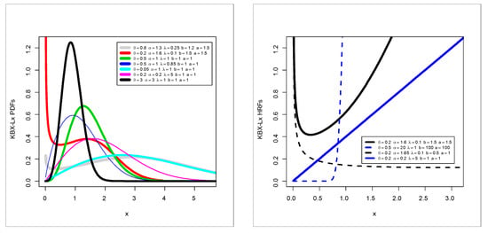
Figure 1.
Probability density function (PDF) plots and HRF plots of the KBX Lomax (Lx) model.
4. Statistical Properties
4.1. Quantile Function
For the KBX quantile function, say can be derived via inverting (2) as
where
4.2. Moments
Let be a nonnegative random variable which has the Exp-G with power parameter . The r moment of the KBX-G family can be obtained from (11) as
where can be calculated and analyzed numerically in terms of the baseline quantile function , i.e., as
For the KBXLx model
where and is the complete beta function. Here, we introduce a formula for the moment generating function (MGF) as
where is the moment generating function (MGF) of . Consequently, we can easily determine from the Exp-G MGF as
which can be calculated numerically from the baseline quantile function, i.e., Thus, for the KBXLx model we have
4.3. Conditional Moments
The s incomplete moments of defined by for any real can be expressed from (11) as
where and and can be evaluated numerically. For the KBXLx
where is the incomplete beta function.
4.4. Mean Deviation
The mean deviations of the mean and the mean deviations of the median
are defined by
and
respectively, where median , and is the first complete moment given by with .
5. Simple Type Copula
5.1. BvKBX Type via FGM Copula
Consider the joint CDF of the FGM family where the marginal function , , is a dependence parameter and for every , which is “grounded minimum” and and which is “grounded maximum” (see [7,8,9,10,11,12]). Then, setting
and
we have
The joint PDF can then derived from or from
5.2. BvKBX Type via Modified FGM Copula
Consider the modified version of FGM copula defined as (see [11]) or where , and . Where and are two functions on with the following conditions:
I The boundary condition:
II Let
Then,
where
and
BvKBX-FGM (Type I) model
Consider , then we get
where and
BvKBX-FGM (Type II) model
Let and be two functional forms to satisfy all the conditions stated earlier where
The corresponding BvKBX-FGM (Type II) can be derived from
BvKBX-FGM (Type III) model
Consider the following functional form for both and which satisfy all the conditions stated earlier where
In this case, one can also derive a closed form expression for the associated CDF of the BivKBX-FGM (Type III).
BvKBX-FGM (Type IV) model
According to [13], the CDF of the BvKBX-FGM (Type IV) model can be derived from
Then,
where and .
5.3. BvKBX Type via Clayton Copula
The Clayton copula can be considered as
Let us assume that KBX and KBX . Then, setting
and
Then, the BvKBX type distribution can be derived as
5.4. BvKBX Type via Renyi’s Entropy
Consider the theorem of [14] where
then, the associated BvKBX will be
By fixing and we then have a five-dimension parameter BvKBX-type distribution.
5.5. MvKBX Extention via Clayton Copula
The -dimensional extension from the above will be
Then, the MvKBX extension can expressed as
where .
6. Maximum Likelihood Estimation
Let be the vector of parameters, then the log-likelihood function for is given by
The components of the score function Setting the nonlinear system of equations equal to zero and solving the equations simultaneously yields the maximum likelihood estimation (MLE) of , where these equations cannot be solved analytically; thus, we use any statistical software to solve these equations.
7. Simulations
To assess of the finite sample behavior of the MaxLEs under the KBXLx model, we will consider and apply the following algorithm:
1—Use
to generate N = 1000 samples of size from the KBXLx distribution;
2—Compute the MaxLEs for the N = 1000 samples.
3—Compute the standard errors (StErs) of the MaxLEs for the N = 1000 samples.
4—Compute the biases and mean squared errors () given for . We repeated these steps for with so computing biases, mean squared errors for and .
Figure 2, Figure 3, Figure 4, Figure 5 and Figure 6 (left panels) prove that the five biases decrease as . Figure 2, Figure 3, Figure 4, Figure 5 and Figure 6 (right panels) prove that the five MSEs decrease as . The red line in Figure 4 means that the bias reached zero. From Figure 2, Figure 3, Figure 4, Figure 5 and Figure 6 (left panels), the biases for each parameter decrease to zero as . From Figure 2, Figure 3, Figure 4, Figure 5 and Figure 6 (right panels), the MSEs decrease to zero as .
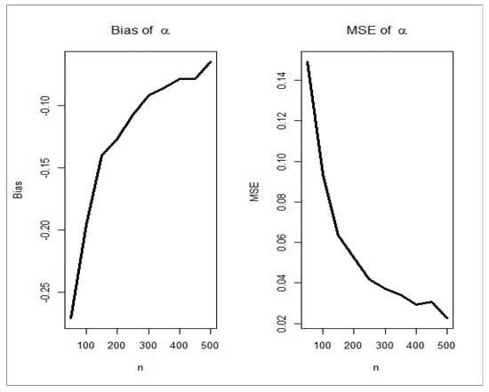
Figure 2.
Bias and MSE for parameter .
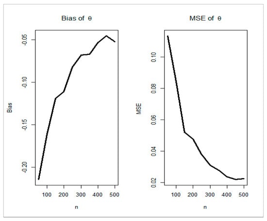
Figure 3.
Bias and MSE for parameter .
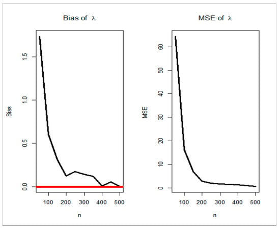
Figure 4.
Bias and MSE for parameter
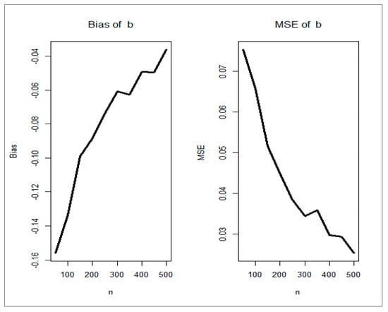
Figure 5.
Bias and MSE for parameter
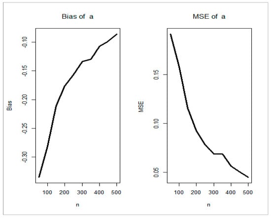
Figure 6.
Bias and MSE for parameter
8. Applications and Comparing Models
In this section, we provide two real-life applications to illustrate the importance, potentiality and flexibility of the KBXLx model. We compare the fit of the KBXLx with some well-known competitive models (see Table 2).

Table 2.
The Competitive Model.
Dataset I (84 Aircraft Windshield): Times of Failure: The first real-life dataset represents the data on times of failure for 84 aircraft windshields (see [15]). The data observations are: 3.7790, 0.0400, 1.248, 2.154, 2.9640, 4.278, 4.449, 1.6190, 2.0100, 2.688, 3.9240, 1.2810, 2.038,2.224, 3.1170, 1.506, 1.866, 2.0850, 2.890, 4.121, 1.3030, 2.089, 2.902, 4.167, 1.4320, 2.097, 2.934, 4.2400, 0.943, 1.9120, 2.632, 3.5950, 1.0700, 1.914, 2.6460, 3.699, 1.1240, 4.376, 2.3850, 3.443, 0.3010, 1.876, 2.820, 3, 4.035, 1.281, 1.480, 2.135, 2.962, 4.2550, 1.505, 2.4810, 3.467, 0.309, 1.8990, 2.610, 3.4780, 0.557, 1.981, 2.661, 2.190, 3.000, 4.3050, 1.568, 2.1940, 3.103, 1.9110, 2.625,3.5780, 1.615, 2.2230, 3.114, 4.485, 1.652, 2.2290, 3.166, 4.570, 1.652, 2.3000, 3.344, 4.602, 1.7570, 2.324, 3.3760, 4.663. Dataset II (63 Aircraft Windshield): Times of Service: The second real-life dataset represents the times of service for 63 aircraft windshields (see [15]). The data observations are: 0.046, 0.622, 1.978, 3.0030, 0.9000, 2.053, 0.2800, 1.794, 3.483, 1.492, 2.600, 0.150, 3.3040, 0.9960, 3.1020, 0.952, 2.065, 0.487, 2.2400, 4.015, 1.183, 2.3410, 2.717, 2.819, 0.3130, 1.915, 2.820, 0.389, 1.9200, 2.878, 1.580, 2.670, 0.248, 1.7190, 1.092, 2.183, 3.695, 1.1520, 3.6220, 1.085, 2.163, 3.6650, 4.628, 1.0030, 2.137, 3.500, 1.0100, 2.141, 1.9630, 2.950, 2.117, 1.436, 2.592, 0.140, 1.2440, 2.435, 4.806, 1.249, 2.4640, 4.881, 1.262, 2.5430, 5.140. See supplementary for detailed data.
Many other useful real-life datasets can be found in [16,17,18,19,20,21,22,23,24,25,26,27]. For exploring the outliers, the box plot is plotted in Figure 7. Based on Figure 7, we note that no outliers were found. For checking the data normality, the Q–Q plot is sketched in Figure 8. Based on Figure 8, we note that normality nearly exists. For exploring the shape of the HRF for real data, the total time test (TTT) plot (see [28]) is provided (see Figure 9). Based on Figure 9, we note that the HRF is “increasing monotonically” for the two real-life datasets. For exploring the initial shape of real data nonparametrically, the KDE is provided in Figure 10. Figure 11 and Figure 12 give the estimated Kaplan–Meier survival (EKMS) plot, estimated PDF (EPDF), P–P plot and estimated HRF (EHRF) for dataset I and II, respectively.
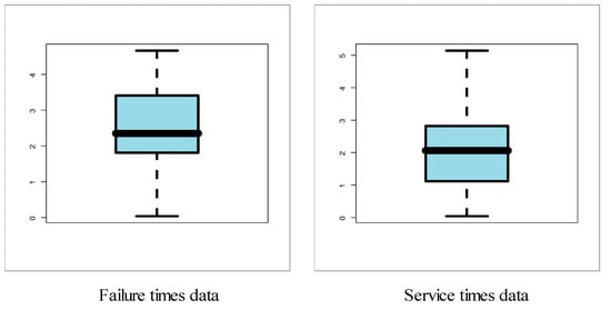
Figure 7.
Box plots.
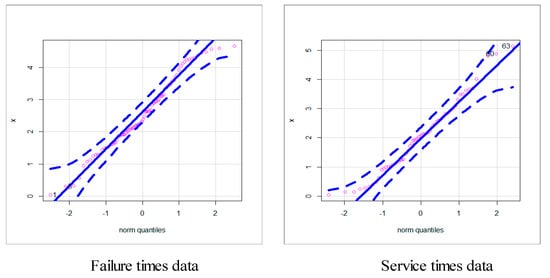
Figure 8.
Normal quantile–quantile (Q–Q) plots.
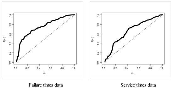
Figure 9.
Total time test (TTT) plots.
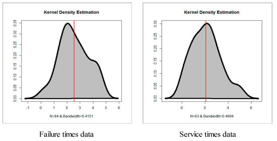
Figure 10.
Nonparametric kernel density estimation (KDE).
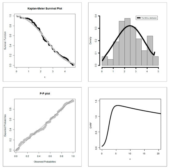
Figure 11.
EKMS plot, EPDF, P–P plot and EHRF for dataset I.
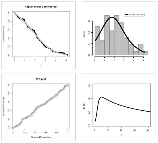
Figure 12.
EKMS plot, EPDF, P–P plot and EHRF for dataset II.
The following goodness-of-fit (GOF) statistics are used: Akaike information criterion (AIC), Bayesian IC (BIC), consistent AIC (CAIC), Hannan–Quinn IC (HQIC), Cramér-von Mises () and Anderson–Darling () for comparing the competitive models. For failure time data, the results are listed in Table 3 and Table 4. Table 3 gives the MaxLEs and StErs for failure time data. Table 4 gives the and GOF statistics for failure time data. For service time data, the analysis results are listed in Table 5 and Table 6. Table 5 gives the MaxLEs and StErs for service time data, and Table 6 gives the and GOFs statistics for the service time data. Based on Table 4 and Table 6, we note that the KBXLx model gives the lowest values for the AIC, CAIC, BIC, HQIC, and among all the fitted models. Hence, it could be chosen as the best model under these criteria.

Table 3.
Maximum Likelihood Estimation (MLEs) and SEs for Failure Time Data.

Table 4.
-ℓ and Goodness-of-Fit (GOF) Statistics for Failure Time Data.

Table 5.
MLEs and SEs for Service Time Data.

Table 6.
-ℓ and GOFs Statistics for Service Time Data.
It is worth mentioning that the presented class of stochastic distributions can have also an important utilization in the insurance industry, risks, reliability, medicine and engineering (see [36,37,38,39,40,41,42,43,44,45,46,47]).
9. Conclusions
A new family of probability distributions based on the Kumaraswamy and Burr X families is derived and studied. Some new bivariate type G families using Farlie–Gumbel–Morgenstern copula, modified Farlie–Gumbel–Morgenstern copula, Clayton copula and Renyi’s entropy copula are derived. Some special models based on exponential, Weibull, Rayleigh, Lomax and Burr XII distributions are presented. Then, special attention is devoted to the Lomax case. Some of its statistical properties, including the quantile function, moments, incomplete moments and mean deviation, are presented. Simulation based on biases and mean squared errors is introduced. Based on this simulation, the maximum likelihood method performs well and can be used for estimating the model parameters. Finally, two real-life applications to illustrate the importance of the new family are proposed.
Supplementary Materials
The first and second datasets are given by [15]. https://onlinelibrary.wiley.com/doi/book/10.1002/047147326X.
Author Contributions
All authors contributed equally for this work. All authors have read and agreed to the published version of the manuscript.
Funding
King Saud University.
Acknowledgments
The authors extend their sincere appreciation to the Deanship of Scientific Research at King Saud University for funding this work through research group No (RG-1438-086).
Conflicts of Interest
The authors declare no conflict of interest
References
- Marshall, A.W.; Olkin, I. A new method for adding a parameter to a family of distributions with application to the exponential and Weibull families. Biometrika 1997, 84, 641–652. [Google Scholar] [CrossRef]
- Eugene, N.; Lee, C.; Famoye, F. Beta-normal distribution and its applications. Commun. Stat. Theory Methods 2002, 31, 497–512. [Google Scholar] [CrossRef]
- Cordeiro, G.M.; de Castro, M. A new family of generalized distributions. J. Stat. Comput. Simul. 2011, 81, 883–893. [Google Scholar] [CrossRef]
- Yousof, H.M.; Afify, A.Z.; Hamedani, G.G.; Aryal, G. The Burr X generator of distributions for lifetime data. J. Stat. Theory Appl. 2017, 16, 288–305. [Google Scholar] [CrossRef]
- Cordeiro, G.M.; Yousof, H.M.; Ramires, T.G.; Ortega, E.M.M. The Burr XII system of densities: Properties, regression model and applications. J. Stat. Comput. Simul. 2018, 88, 432–456. [Google Scholar] [CrossRef]
- Yousof, H.M.; Majumder, M.; Jahanshahi, S.M.A.; Ali, M.M.; Hamedani, G.G. A new Weibull class of distributions: Theory, characterizations and applications. J. Stat. Res. Iran 2018, 15, 45–83. [Google Scholar] [CrossRef]
- Fisher, N.I. Copulas. In Encyclopedia of Statistical Sciences, Updated Volume 1; Kotz, S., Read, C.B., Banks, D.L., Eds.; John Wiley and Sons: New York, NY, USA, 1997; pp. 159–164. [Google Scholar]
- Farlie, D.J.G. The performance of some correlation coefficients for a general bivariate distribution. Biometrika 1960, 47, 307–323. [Google Scholar] [CrossRef]
- Morgenstern, D. Einfache beispiele zweidimensionaler verteilungen. Mitteilingsblatt Math. Stat. 1965, 8, 234–235. [Google Scholar]
- Gumbel, E.J. Bivariate exponential distributions. J. Am. Stat. Assoc. 1960, 55, 698–707. [Google Scholar] [CrossRef]
- Gumbel, E.J. Bivariate logistic distributions. J. Am. Stat. Assoc. 1961, 56, 335–349. [Google Scholar] [CrossRef]
- Rodriguez-Lallena, J.A.; Ubeda-Flores, M. A new class of bivariate copulas. Stat. Probab. Lett. 2004, 66, 315–325. [Google Scholar] [CrossRef]
- Ghosh, I.; Ray, S. Some alternative bivariate Kumaraswamy type distributions via copula with application in risk management. J. Stat. Theory Pract. 2016, 10, 693–706. [Google Scholar] [CrossRef]
- Pougaza, D.B.; Djafari, M.A. Maximum Entropies Copulas. In Proceedings of the 30th International Workshop on Bayesian Inference and Maximum Entropy Methods in Science and Engineering, Chamonix, France, 4–9 July 2010; AIP Press: College Park, MD, USA, 2011; pp. 329–336. [Google Scholar]
- Murthy, D.N.P.; Xie, M.; Jiang, R. Weibull Models; Wiley: Hoboken, NJ, USA, 2004. [Google Scholar]
- Aryal, G.R.; Ortega, E.M.; Hamedani, G.G.; Yousof, H.M. The Topp Leone Generated Weibull distribution: Regression model, characterizations and applications. Int. J. Stat. Probab. 2017, 6, 126–141. [Google Scholar] [CrossRef]
- Yousof, H.M.; Altun, E.; Ramires, T.G.; Alizadeh, M.; Rasekhi, M. A new family of distributions with properties, regression models and applications. J. Stat. Manag. Syst. 2018, 21, 163–188. [Google Scholar] [CrossRef]
- Elbiely, M.M.; Yousof, H.M. A New Extension of the Lomax Distribution and its Applications. J. Stat. Appl. 2018, 2, 18–34. [Google Scholar]
- Altun, E.; Yousof, H.M.; Chakraborty, S.; Handique, L. Zografos-Balakrishnan Burr XII distribution: Regression modeling and applications. Int. J. Math. Stat. 2018, 19, 46–70. [Google Scholar]
- Ibrahim, M.; Yousof, H.M. A new generalized Lomax model: Statistical properties and applications. J. Data Sci. 2020, 18, 190–217. [Google Scholar]
- Ibrahim, M. A new extended Fréchet distribution: Properties and estimation. Pak. J. Stat. Oper. Res. 2019, 15, 773–796. [Google Scholar]
- Ibrahim, M. The compound Poisson Rayleigh Burr XII distribution: Properties and applications. J. Appl. Probab. Stat. 2020, 15, 73–97. [Google Scholar]
- Ibrahim, M. The generalized odd Log-logistic Nadarajah Haghighi distribution: Statistical properties and different methods of estimation. J. Appl. Probab. Stat. 2020, 15, 61–84. [Google Scholar]
- Yadav, A.S.; Goual, H.; Alotaibi, R.M.; Rezk, H.; Ali, M.M.; Yousof, H.M. Validation of the Topp-Leone-Lomax model via a modified Nikulin-Rao-Robson GOF test with different methods of estimation. Symmetry 2020, 12, 57. [Google Scholar] [CrossRef]
- Mansour, M.; Yousof, H.M.; Shehata, W.A.M.; Ibrahim, M. A new two parameter Burr XII distribution: Properties, copula, different estimation methods and modeling acute bone cancer data. J. Nonlinear Sci. Appl. 2020, 13, 223–238. [Google Scholar] [CrossRef]
- Goual, H.; Yousof, H.M. Validation of Burr XII inverse Rayleigh model via a modified chi squared GOF test. J. Appl. Stat. 2019, 47, 1–32. [Google Scholar]
- Goual, H.; Yousof, H.M.; Ali, M.M. Lomax inverse Weibull model: Properties, applications and a modified Chi-squared GOF test for validation. J. Nonlinear Sci. Appl. 2020, 13, 330–353. [Google Scholar] [CrossRef]
- Aarset, M.V. How to identify a bathtub hazard rate. IEEE Trans. Reliab. 1987, 36, 106–108. [Google Scholar] [CrossRef]
- Khalil, M.G.; Hamedani, G.G.; Yousof, H.M. The Burr X exponentiated Weibull model: Characterizations, mathematical properties and applications to failure and survival times data. Pak. J. Stat. Oper. Res. 2019, XV, 141–160. [Google Scholar] [CrossRef]
- Altun, E.; Yousof, H.M.; Hamedani, G.G. A new log-location regression model with influence diagnostics and residual analysis. Facta Univ. Ser. Math. Inform. 2018, 33, 417–449. [Google Scholar]
- Yousof, H.M.; Alizadeh, M.; Jahanshahiand, S.M.A.; Ramires, T.G.; Ghosh, I.; Hamedani, G.G. The transmuted Topp-Leone G family of distributions: Theory, characterizations and applications. J. Data Sci. 2017, 15, 723–740. [Google Scholar]
- Cordeiro, G.M.; Ortega, E.M.; Popovic, B.V. The gamma-Lomax distribution. J. Stat. Comput. Simul. 2015, 85, 305–319. [Google Scholar] [CrossRef]
- Lemonte, A.J.; Cordeiro, G.M. An extended Lomax distribution. Statistics 2013, 47, 800–816. [Google Scholar] [CrossRef]
- Gupta, R.C.; Gupta, P.L.; Gupta, R.D. Modeling failure time data by Lehman alternatives. Commun. Stat. Theory Methods 1998, 27, 887–904. [Google Scholar] [CrossRef]
- Lomax, K.S. Business failures: Another example of the analysis of failure data. J. Am. Stat. Assoc. 1954, 49, 847–852. [Google Scholar] [CrossRef]
- Pešta, M.; Okhrin, O. Conditional least squares and copulae in claims reserving for a single line of business. Insur. Math. Econ. 2014, 56, 28–37. [Google Scholar] [CrossRef]
- Peštová, B.; Pešta, M. Change point estimation in panel data without boundary issue. Risks 2017, 5, 7. [Google Scholar] [CrossRef]
- Hamedani, G.G.; Yousof, H.M.; Rasekhi, M.; Alizadeh, M.; Najibi, S.M. Type I general exponential class of distributions. Pak. J. Stat. Oper. Res. 2017, 14, 39–55. [Google Scholar] [CrossRef][Green Version]
- Mansour, M.; Korkmaz, M.Ç.; Ali, M.M.; Yousof, H.M.; Ansari, S.I.; Ibrahim, M. A generalization of the exponentiated Weibull model with properties, Copula and application. Eurasian Bull. Math. 2020, 3, 84–102. [Google Scholar]
- Korkmaz, M.C.; Yousof, H.M.; Hamedani, G.G.; Ali, M.M. The Marshall-Olkin generalized G Poisson family of distributions. Pak. J. Stat. 2018, 34, 251–267. [Google Scholar]
- Hamedani, G.G.; Altun, E.; Korkmaz, M.C.; Yousof, H.M.; Butt, N.S. A new extended G family of continuous distributions with mathematical properties, characterizations and regression modeling. Pak. J. Stat. Oper. Res. 2018, 14, 737–758. [Google Scholar] [CrossRef]
- Hamedani, G.G.; Rasekhi, M.; Najibi, S.M.; Yousof, H.M.; Alizadeh, M. Type II general exponential class of distributions. Pak. J. Stat. Oper. Res. 2019, 15, 503–523. [Google Scholar] [CrossRef]
- Korkmaz, M.C.; Altun, E.; Yousof, H.M.; Hamedani, G.G. The odd power Lindley generator of probability distributions: Properties, characterizations and regression modeling. Int. J. Stat. Probab. 2019, 8, 70–89. [Google Scholar]
- Nascimento, A.D.C.; Silva, K.F.; Cordeiro, G.M.; Alizadeh, M.; Yousof, H.M. The odd Nadarajah-Haghighi family of distributions: Properties and applications. Stud. Sci. Math. Hung. 2019, 56, 1–26. [Google Scholar] [CrossRef]
- Elsayed, H.A.H.; Yousof, H.M. The generalized odd generalized exponential Fréchet model: univariate, bivariate and multivariate extensions with properties and applications to the univariate version. Pak. J. Stat. Oper. Res. 2020, 16, 529–544. [Google Scholar] [CrossRef]
- Ibrahim, M.; Yousof, H.M. Transmuted Topp-Leone Weibull Lifetime Distribution: Statistical Properties and Different Method of Estimation. Pak. J. Stat. Oper. Res. 2020, 16, 501–515. [Google Scholar] [CrossRef]
- Ibrahim, M.; Mohammed, W.S.; Yousof, H.M. Bayesian and Classical Estimation for the One Parameter Double Lindley Model. Pak. J. Stat. Oper. Res. 2020, 16, 409–420. [Google Scholar]
© 2020 by the authors. Licensee MDPI, Basel, Switzerland. This article is an open access article distributed under the terms and conditions of the Creative Commons Attribution (CC BY) license (http://creativecommons.org/licenses/by/4.0/).