A New Multi-Sensor Fusion Target Recognition Method Based on Complementarity Analysis and Neutrosophic Set

Abstract

To improve the efficiency, accuracy, and intelligence of target detection and recognition, multi-sensor information fusion technology has broad application prospects in many aspects. Compared with single sensor, multi-sensor data contains more target information and effective fusion of multi-source information can improve the accuracy of target recognition. However, the recognition capabilities of different sensors are different during target recognition, and the complementarity between sensors needs to be analyzed during information fusion. This paper proposes a multi-sensor fusion recognition method based on complementarity analysis and neutrosophic set. The proposed method mainly has two parts: complementarity analysis and data fusion. Complementarity analysis applies the trained multi-sensor to extract the features of the verification set into the sensor, and obtain the recognition result of the verification set. Based on recognition result, the multi-sensor complementarity vector is obtained. Then the sensor output the recognition probability and the complementarity vector are used to generate multiple neutrosophic sets. Next, the generated neutrosophic sets are merged within the group through the simplified neutrosophic weighted average (SNWA) operator. Finally, the neutrosophic set is converted into crisp number, and the maximum value is the recognition result. The practicality and effectiveness of the proposed method in this paper are demonstrated through examples.

1. Introduction

In daily life, target recognition involves all aspects of our lives, such as intelligent video surveillance and face recognition. These applications also make target recognition technology more popular. The development of related technologies has greatly enriched the application scenarios of target recognition and tracking theories. Research on related theoretical methods has also received extensively attention. Target recognition involves image processing, calculation computer vision, pattern recognition and other subjects.

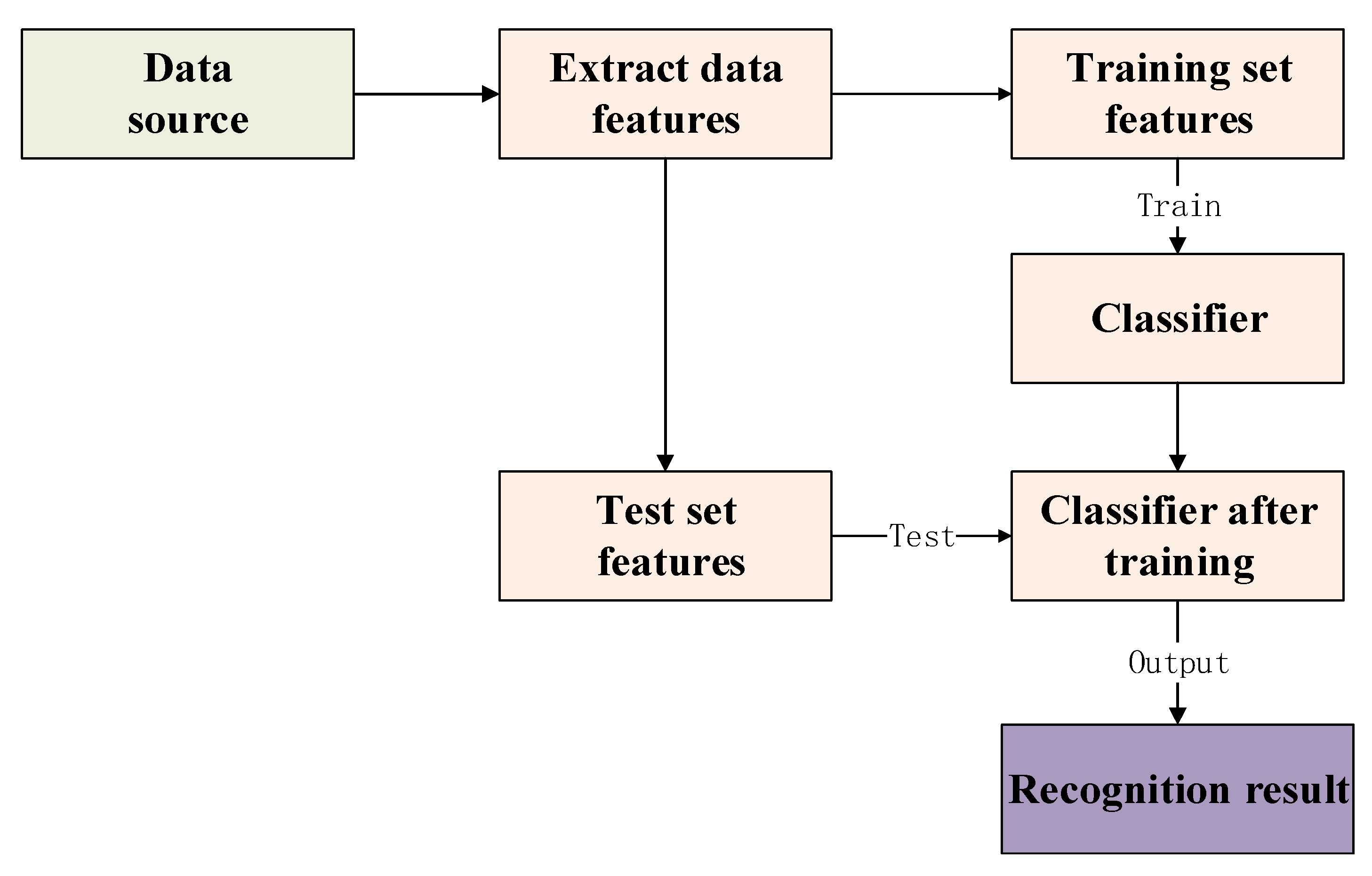
Generalized target recognition includes two stages, feature extraction, and classifier classification. Through feature extraction, image, video, and other target observation data are preprocessed to extract feature information, and then the classifier algorithm implements target classification based on the feature information [1]. Common image features can be divided into color gray statistical feature, texture edge feature, algebraic feature, and variation coefficient feature. The feature extraction methods corresponding to the above features are color histogram, gray-level co-occurrence matrix method, principal component analysis method, wavelet transform [2]. The classic target classification algorithms include decision tree, support vector machine [3], neural network [4], logistic regression, and naive Bayes classification [5,6,7,8]. On the basis of a single classifier, the ensemble classifier integrates the classification results of a series of weak classifiers through an ensemble learning method, so as to obtain a better classification effect than a single classifier, mainly including Bagging and Boosting [9]. With the development of high-performance computing equipment and the enlargement in the amount of available data, deep learning related theories and methods have developed rapidly, and the application of deep learning in the direction of target recognition has also made it break through the limitations of traditional methods based on deep neural networks [10,11,12]. Classification network models include LeNet, AlexNet, VggNet.

In practical applications, multi-source sensor data is often processed in decision analysis [13,14,15,16,17,18,19] as the number of sensors increases. For the problem of uncertain information processing, there are many theoretical methods such as Dempster-Shafer evidence theory [20,21,22,23,24,25,26], fuzzy set theory [27,28], D number [29,30,31,32] and rough set theory [33].

Smarandache [34] firstly generalized the concepts of fuzzy sets [35], intuitionistic fuzzy sets (IFS) [36] and interval-valued intuitionistic fuzzy sets (IVIFS) [37], and proposed the neutrosophic set. It is very suitable to use the neutrosophic set to deal with uncertain and inconsistent information in the real world. However, its authenticity, uncertainty, and false membership function are defined in the real number standard or non-standard subset. Therefore, non-standard intervals are not suitable for scientific and engineering applications. Therefore, Ye [38] introduced a simplified neutrosophic set (SNS), which limits the true value, uncertainty, and false membership function to the actual standard interval $[0,1]$. In addition, SNS also includes single value neutrosophic set (SVNS) [39,40,41] and interval neutrosophic set (INS) [42].

As a new kind of fuzzy set, neutrosophic set [43,44] have been used in many fields, such as decision-making [45,46,47,48], data analysis [49,50], fault diagnosis [51], the shortest path problem [52]. There is also a lot of progress in the related theoretical research of neutrosophic set. For example, score function of pentagonal neutrosophic set [53,54].

Existing multi-sensor fusion methods, such as evidence theory, have complex calculation and long calculation time [55], and there are a few methods that use neutrosophic set in multi-sensor fusion. Therefore, this paper proposes a multi-sensor fusion based on neutrosophic set. First, the complementarity vectors between multiple sensors are calculated. Then these complementarity vectors and the probability of sensor output are used to form a group of neutrosophic sets, and generated neutrosophic sets are fused through the SNWA operator. Finally, the neutrosophic set is converted to the crisp number, and the maximum value is the recognition result. The proposed method has simple calculation and fast operation, and can effectively improve the accuracy of target recognition.

The rest of this article is organized as follows: Section 2 introduces some necessary concepts, such as neutrosophic set and multi-category evaluation standard. The proposed multi-sensor fusion recognition method is listed step by step in Section 3. In Section 4, an example is used to illustrate and explain the effective of proposed method. Some results discussion are shown in Section 5.

2. Preliminaries

2.1. Neutrosophic Set

Definition 1.

The the simplified neutrosophic set (SNS) is defined as follows [38]:

X is a finite set, with a element of X denoted by x. A neutrosophic set (A) in X contains three parts: a truth-membership function $\left(T_p\right)$, an indeterminacy-membership function $\left(I_p\right)$, and a falsity-membership function $\left(F_p\right)$.

$$\begin{array}{cc}\hfill & 0\le T_P\left(x\right)\le 1\hfill \end{array}$$

(1)

$$\begin{array}{cc}\hfill & 0\le I_P\left(x\right)\le 1\hfill \end{array}$$

(2)

$$\begin{array}{cc}\hfill & 0\le F_P\left(x\right)\le 1\hfill \end{array}$$

(3)

$$\begin{array}{cc}\hfill & 0\le T_P\left(x\right)+I_P\left(x\right)+F_P\left(x\right)\le 3\hfill \end{array}$$

(4)

A single-valued neutrosophic set P on X is defined as:

$$P=\left\{\langle x,T_P\left(x\right),I_P\left(x\right),F_P\left(x\right)\rangle \right|x\in X\}$$

(5)

This is called a SNS. In particular, if X includes only one element, $N=\langle x,T_P\left(x\right),I_P\left(x\right),F_P\left(x\right)\rangle$ is called a SNN (the simplified neutrosophic number) and is denoted by $\alpha =〈\mu ,\pi ,\nu 〉$. The numbers $\mu ,\pi ,\nu$ denote the degree of membership, the degree of indeterminacy-membership, and the degree of non-membership.

Definition 2.

The crisp number of each SNN is deneutrosophicated and calculated as follows [56]:

$$S_i={\mu }_i+\left({\pi }_i\right)\times (\frac{{\mu }_i}{{\mu }_i+{\nu }_i})$$

(6)

$S_i$ can be regarded as the score of SNN, so SNN can be sorted according to crisp number $S_i$.

2.2. Commonly Used Evaluation Indicators for Multi-Classification Problems

The index for evaluating the performance of a classifier is generally the accuracy of the classifier, which is defined as the ratio of the number of samples correctly classified by the classifier to the total number of samples for a given test data set [57].

The commonly used evaluation indicators for classification problems are precision and recall. Usually, the category of interest is regarded as the positive category, and the other categories are regarded as the negative category. The prediction of the classifier on the test data set is correct or incorrect. There are four situations as follows:

• True Positive(TP): The true category is a positive example, and the predicted category is a positive example.
• False Positive (FP): The true category is negative, and the predicted category is positive.
• False Negative (FN): The true category is positive, and the predicted category is negative.
• True Negative (TN): The true category is negative, and the predicted category is negative.

Based on the above basic concepts, the commonly used evaluation indicators for multi-classification problems are as follows.

• Precision or precision rate, also known as precision (P):

  $$P=\frac{TP}{TP+FP}$$

  (7)
• Recall rate, also known as recall rate (R):

  $$R=\frac{TP}{TP+FN}$$

  (8)
• F1 score is an index used to measure the accuracy of the classification model. It also takes into account the accuracy and recall of the classification model. The score can be regarded as a harmonic average of model accuracy and recall. Its maximum value is 1 and its minimum value is 0:

  $$F_1=\frac{2\times P\times R}{P+R}$$

  (9)

2.3. AdaBoost Algorithm

AdaBoost is essentially an iterative algorithm [58], and its core idea is to train some weak classifier $h_i$ based on the initial sample using the decision tree algorithm. Use the classifier to detect the sample set. For each training sample point, adjust its weight according to whether the result of its classification is accurate: if $h_i$ makes it classified correctly, reduce the weight of the sample point; otherwise, increase the sample the weight of the point. The adjusted weight is calculated according to the accuracy of the detection result. The sample set after adjusting the weight constitutes the sample set to be trained at the next level, which is used to train the next level classifier. In this way, iterate step by step to obtain a new classifier until the classifier $h_m$ is obtained, and the sample detection error rate is 0.

Combine $h_1,h_2,\dots ,h_m$ according to the error rate of the sample detection: make the weak classifier with the larger error account for the smaller weight in the combined classifier, and the weak classifier with the smaller error account for the larger weight to obtain a combined classifier.

The algorithm is essentially a comprehensive improvement of the weak classifier trained by the basic decision tree algorithm. Through continuous training of samples and weight adjustment, multiple classifiers are obtained, and the classifiers are combined by weight to obtain a comprehensive classifier that improves the ability of data classification. The whole process is as follows:

• Train weak classifiers with sample sets.
• Calculate the error rate of the weak classifier, and obtain the correct and incorrect sample sets.
• Adjust the sample set weight according to the classification result to obtain a redistributed sample set.

After M cycles, M weak classifiers are obtained, and the joint weight of the classifier is calculated according to the detection accuracy of each weak classifier, and finally a strong classifier is obtained.

2.4. HOG Feature

Histogram of oriented gradient (HOG), which is a feature descriptor for target detection. This technology counts the number of directional gradients that appear locally in the image. This method is similar to the histogram of edge orientation and scale-invariant feature transform, but the difference is hog calculate the density matrix based on the uniform space to improve accuracy. Navneet Dalal and Bill Triggs first proposed HOG in 2005 for pedestrian detection in static images or videos [59].

The core idea of HOG is that the shape of the detected local object can be described by the light intensity gradient or the distribution of the edge direction. By dividing the entire image into small connected areas (called cells). Each cell generates a directional gradient histogram or the edge direction of the pixel in the cell, and the descriptor is represented by combining the histogram. To improve the accuracy, the local histogram can be compared and standardized by calculating the light intensity of a larger area (called block) in the image as a measure, and then using this value (measure) to normalize all cells in the block. This normalization process completes better illumination/shadow invariance. Compared with other descriptors, the descriptors obtained by HOG maintain the invariance of geometric and optical transformations (unless the object orientation changes).

2.5. Gabor Feature

Gabor feature [60] is a feature that can be used to describe the texture information of an image. The frequency and direction of the Gabor filter are similar to the human visual system, and it is particularly suitable for texture representation and discrimination. The Gabor feature mainly relies on the Gabor kernel to window the signal in the frequency domain, so as to describe the local frequency information of the signal.

In terms of feature extraction, Gabor wavelet transform is compared with other methods: on the one hand, it processes less data and can meet the real-time requirements of the system; on the other hand, wavelet transform is insensitive to changes in illumination and can tolerate a certain degree of when image rotation and deformation are used for recognition based on Euclidean distance, the feature pattern and the feature to be measured do not need to correspond strictly, so the robustness of the system can be improved.

2.6. D-AHP Theory

Analytic Hierarchy Process (AHP) [61] is a systematic and hierarchical analysis method that combines qualitative and quantitative analysis. The characteristic of this method is that on the basis of in-depth research on the nature, influencing factors and internal relations of complex decision-making problems, it uses less quantitative information to mathematicize the thinking process of decision-making, thereby providing multi-objective, multi-criteria or complex decision-making problems with no structural characteristics provide simple decision-making methods.

The D-AHP method extends the traditional AHP method in theory. In the D-AHP method [62], the derived results about the ranking and priority weights of alternatives are impacted by the credibility of providing information. A parameter $\lambda$ is used to express the credibility of information, and its value is associated with the cognitive ability of experts. If the comparison information used in the decision-making process is provided by an authoritative expert, $\lambda$ will take a smaller value. If the comparison information comes from an expert whose judgment is with low belief, $\lambda$ takes a higher value.

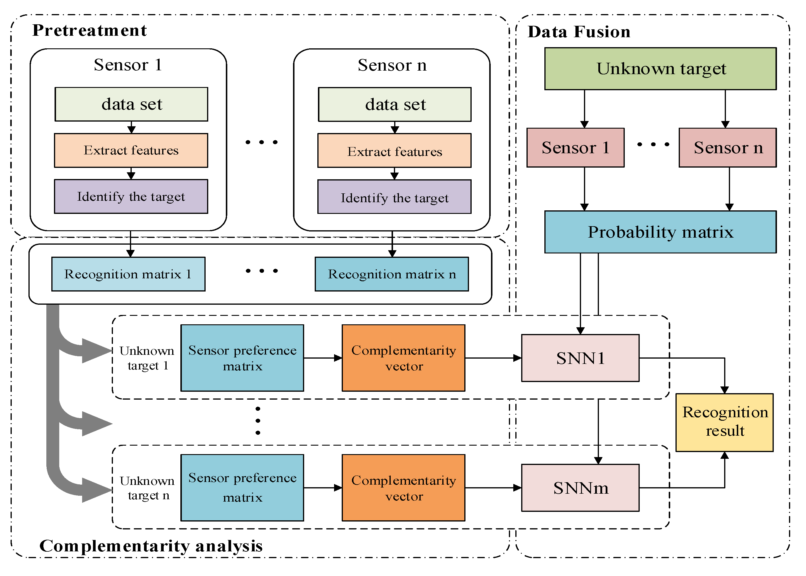
3. The Proposed Method

In general sensor recognition, the training set is inputting to train the sensor by extracting feature, and then the test set is inputting to test and get the recognition result. To improve the accuracy of multi-sensor fusion recognition, this paper proposes a fusion recognition method based on neutrosophic set. The proposed method in this paper is mainly divided into two parts: complementarity analysis and data fusion. The main steps of the method proposed in this paper are shown in Figure 1.

The essence of complementarity is to calculate the weight of the recognition ability of the base sensor in different categories. Based on this, the data set is divided into training set, validation set, and test set. First, the base sensor preference matrix is obtained from the recognition matrix of the trained base sensor on the verification set, and then the sensor complementarity vector is calculated in each category.

Data fusion aims at different target types, based on the sensor complementarity vector, the recognition results of different sensors are generated by the neutrosophic set. Then the fusion of the neutrosophic set can be obtained in different categories, and finally the neutrosophic set is converted into crisp number, and the maximum value is taken as the recognition result.

3.1. Complementarity

The main steps of the multi-sensor complementarity analysis are proposed as follows:

• According to the data test result, the sensor recognition matrix can be obtained.
• The sensor preference matrix for different target types is obtained from multiple sensor recognition matrices.
• The sensor complementarity vector is gotten from the sensor preference relationship matrix.

3.1.1. Sensor Recognition Matrix

Suppose there are n types of sensors $X_1,X_2,X_3,\cdots ,X_n$, and m types of target types $Y_1,Y_2,Y_3,\cdots ,Y_m$. For a certain data set i, the recognition results of all its samples can be represented by the following recognition matrix $R_i$.

$$R_i=\left[\begin{array}{cccc}{r^i}_{11}& {r^i}_{12}& ···& {r^i}_{1m}\\ {r^i}_{21}& {r^i}_{22}& \cdots & {r^i}_{2m}\\ ⋮& ⋮& \ddots & ⋮\\ {r^i}_{n1}& {r^i}_{n2}& \cdots & {r^i}_{nm}\end{array}\right]$$

(10)

3.1.2. Sensor Preference Matrix

To obtain the preference relationship matrix between sensors, the preference between sensors needs to be defined. For two sensors, if the recognition performance of the sensor $X_1$ on the target $Y_j$ is better than the recognition performance of the sensor $X_2$, then for the target $Y_j$, the sensor $X_1$ is better than the sensor $X_2$. The recognition results of a certain sensor on the samples in the data set i can be organized in the form of a recognition matrix, but the rows and columns become the recognized category of the sample and the true category of the sample. Furthermore, for the target of category $Y_j$, according to the recognition matrix, we can get

Table 1. $R_j^i$: The recognition situation of a certain sensor to the target of category $Y_j$.

Real-Recognition	${\mathit{Y}}_{\mathit{j}}$	Non-${\mathit{Y}}_{\mathit{j}}$
$Y_j$	${r^i}_{jj}$	${\displaystyle {\displaystyle \sum }_{k\ne j}}{r^i}_{jk}$
non-$Y_j$	${\displaystyle {\displaystyle \sum }_{k\ne j}}{r^i}_{kj}$	${\displaystyle {\displaystyle \sum }_{l\ne j}}{\displaystyle {\displaystyle \sum }_{k\ne j}}{r^i}_{kl}$

:

Record the above matrix as $R_j^i$ in Table 1, where ${r^i}_{jj}$ is the number of correct recognition of the category $Y_j$ by the sensor, ${\displaystyle {\displaystyle \sum }_{k\ne j}}{r^i}_{kj}$ is the number of samples that the sensor misrecognizes non-targets. ${\displaystyle {\displaystyle \sum }_{k\ne j}}{r^i}_{jk}$ is the number of misrecognized category $Y_j$ samples into other categories. ${\displaystyle {\displaystyle \sum }_{l\ne j}}{\displaystyle {\displaystyle \sum }_{k\ne j}}{r^i}_{kl}$ is the number of samples other than the above three cases number. If the optimal performance of sensor recognition is expressed as a matrix:

$$I_j=\left[\begin{array}{cc}{\displaystyle {\displaystyle \sum }_{l=1}^h}{r}_{jl}^i& 0\\ 0& {\displaystyle {\displaystyle \sum }_{k\ne j}}{\displaystyle {\displaystyle \sum }_{l=1}^h}{r}_{kl}^i\end{array}\right]$$

(11)

Which means the category is fully recognized correctly. Then the recognition performance of this sensor to the category $Y_j$ is defined as $\frac{1}{∥R_j^i-I_j∥}$. Therefore, if there are two sensors $X_k$ and $X_l$, the preference value of the recognition accuracy rate of $X_k$ versus $X_l$ in the category (representing the priority of the recognition ability of $X_k$ over $X_l$ in the category of $Y_j$) is defined as:

$${p^j}_{kl}=\frac{\frac{1}{∥{R^k}_j-I_j∥}}{\frac{1}{∥{R^k}_j-I_j∥}+\frac{1}{∥{R^l}_j-I_j∥}}=\frac{∥{R^l}_j-I_j∥}{∥{R^k}_j-I_j∥+∥{R^l}_j-I_j∥}$$

(12)

In the same way, the recognition accuracy preference value of sensor $X_l$ vs $X_k$ on category $Y_j$ is defined as follows:

$${p^j}_{lk}=\frac{∥{R^k}_j-I_j∥}{∥{R^k}_j-I_j∥+∥{R^l}_j-I_j∥}$$

(13)

It is easy to get from the above two formulas that ${p^j}_{kl}+{p^j}_{lk}=1$, which is the sum of the two preference values is 1. If $l=k$, then ${p^j}_{kl}=0.5$. For the case where multiple sensors recognize at the same time, the preference relationship matrix $P^j$ on the category $Y_j$ can be obtained. For each target category in the data set i, a corresponding preference relationship matrix can be obtained.

3.1.3. Sensor Complementarity Vector

Next, using the method in D-AHP theory [62], the complementarity vector can be calculated by the preference relationship matrix.

According to the classifier preference relation matrix $P_j$ of category $Y_j$.

$$P^j=\left[\begin{array}{cccc}{P^j}_{11}& {P^j}_{12}& ···& {P^j}_{1n}\\ {P^j}_{21}& {P^j}_{22}& \cdots & {P^j}_{2n}\\ ⋮& ⋮& \ddots & ⋮\\ {P^j}_{n1}& {P^j}_{n2}& \cdots & {P^j}_{nn}\end{array}\right]$$

(14)

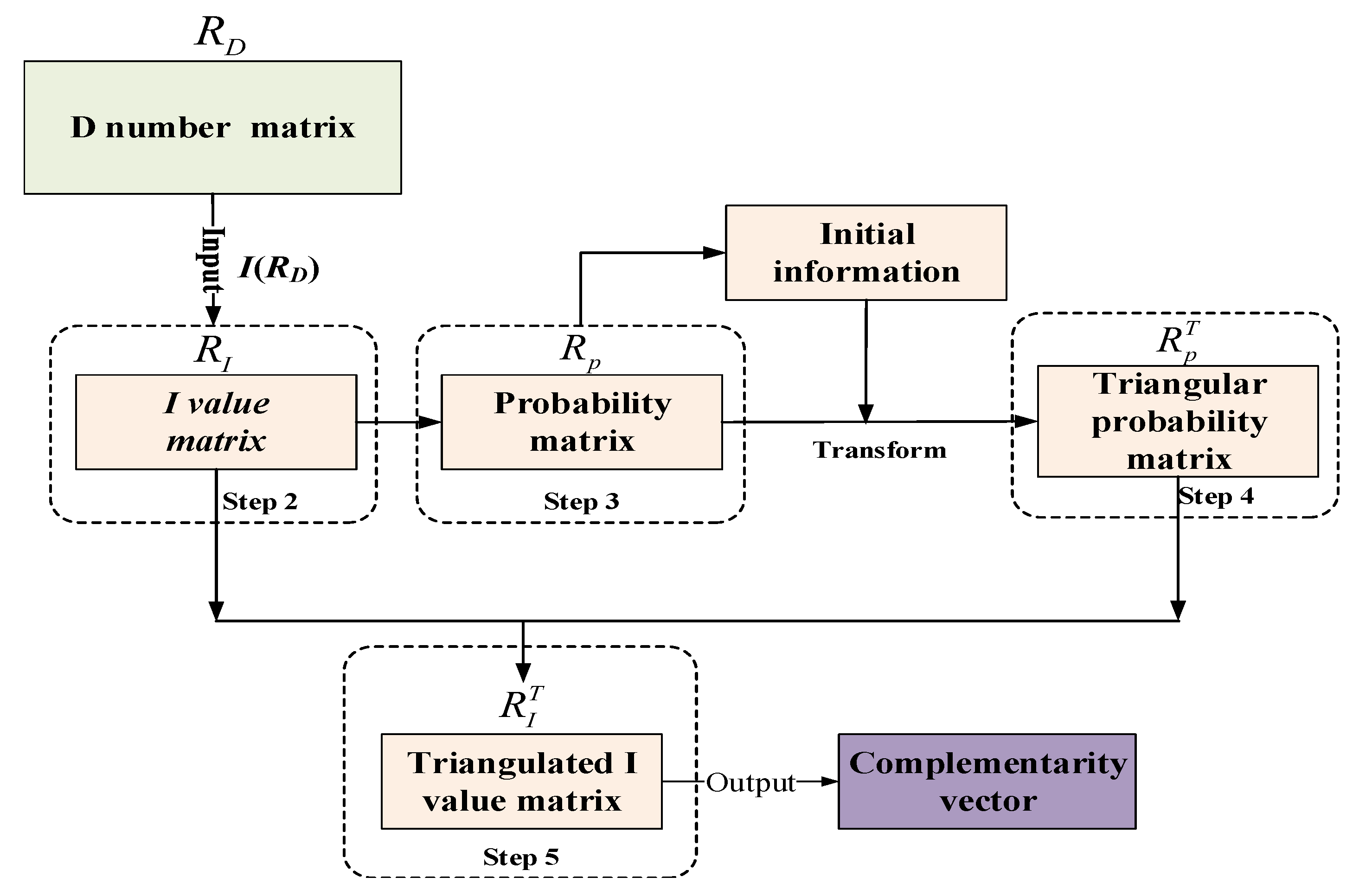
It is calculated that for each sensor complementarity vector $C^j$ of category $Y_j$, $C^j$ is a $1\times n$ dimensional vector. The flowchart of the $C^j$ calculation is presented as Figure 2, the calculation steps are as follows:

• Express the importance of the index relative to the evaluation target through the preference relationship, and construct the D number preference matrix $R_D$.
• According to the integrated representation of the D number, transform the D number preference matrix into a certain number matrix $R_I$.
• Construct a probability matrix $R_I$ based on the deterministic number matrix $R_P$, and calculate the preference probability between the indicators compared in pairs.
• Convert the probability matrix $R_P$ into a triangularized probability matrix ${R^T}_P$, and sort the indicators according to their importance.
• According to the index sorting result, the deterministic number matrix $R_I$ is expressed as a matrix ${R^T}_I$, finally $C^j$ is obtained.

3.2. Data Fusion

For a picture with unknown target type, the probability matrix is formed via the recognition result vectors of each sensor.

$$Q=\left[\begin{array}{ccc}{q}_{11}& \cdots & q_{1m}\\ ⋮& \ddots & ⋮\\ q_{n1}& \cdots & q_{nm}\end{array}\right]$$

(15)

where $q_{ij}$ is the probability that the sensor $X_i$ considers the unknown target as the target type $Y_j$.

At this time, the complementary vector is normalized to obtain the weight coefficient:

$$H^j=C^j/({C^j}_{min}+{C^j}_{max})$$

(16)

If the target type is $Y_j$, the complementarity vector $H^j$ and Q can be combined to obtain a neutrosophic set $\alpha =〈\mu ,\pi ,\nu 〉$. Since there are n sensors, n groups neutrosophic sets can be obtained according to Q and $Y_j$ as follows:

$${\alpha }_i=[\mu =q_{ij}\times H_j,\pi =(1-q_{ij})\times H_j,\nu =1-H_j]$$

(17)

Combining n groups of neutrosophic sets, a group of fused neutrosophic set can be obtianed, and the target recognition neutrosophic set is calculated under the imaginary target type $Y_j$. Since there are m types of target, we can finally use the SNWA operator [63] to get m neutrosophic sets:

$${\alpha }_{Ti}=W_1\times {\alpha }_1+W_2\times {\alpha }_2+\cdots +W_n\times {\alpha }_n={[1-\prod _{i=1}^n(1-{\mu }_i)}^{W_i},\prod _{i=1}^n{\left({\pi }_i\right)}^{W_i},\prod _{i=1}^n{\left({\nu }_i\right)}^{W_i}]$$

(18)

Finally, convert these m SNNs into crisp numbers, and take the maximum value as the recognition result.

$$RS=Max\left(S\right)=Max[S_1={\mu }_{T_1}+({\pi }_{T_1})\times (\frac{{\mu }_{T_1}}{{\mu }_{T_1}+{\nu }_{T_1}}),\dots ,S_m={\mu }_{T_m}+\left({\pi }_{T_m}\right)\times (\frac{{\mu }_{T_m}}{{\mu }_{T_m}+{\nu }_{T_m}})]$$

(19)

4. Simulation

4.1. Data Set

The data source type of the experiment consists of two types: visible light image and infrared light image. There are four target types: sailboat (1), cargo ship (2), speed boat (3), and fishing boat (4). The structure of the experimental data is shown in

Table 2. Target recognition image of infrared data.

Infrared Light Data	Train Set	Validation Set	Test Set
Sailboat	65	28	28
Cargo ship	68	35	35
Speed boat	63	25	25
Fishing boat	79	35	35

and

Table 3. Target recognition image of visible light data.

Visible Light Data	Train Set	Validation Set	Test Set
Sailboat	65	28	28
Cargo ship	79	35	35
Speed boat	70	25	25
Fishing boat	78	35	35

. The data consists of a train set, a verification set, and a test set. The verification set and the test set are the same pictures. Since the information of visible light and infrared sensors needs to be fused in the verification set and test set, two visible and infrared images taken at the same location are required for the same target, as shown in Figure 3, Figure 4, Figure 5 and Figure 6. Due to the lack of data, K = 8 cross-validation is used for verificating and testing. This means that the validation set (test set) is divided into eight groups, and when a certain one group is tested, the remaining seven groups are used as the validation set. The image features use Gabor and HOG, and the classifier uses AdaBoost.

4.2. Sensor

Two data sources (visible light, infrared), two image features (HOG, Gabor), and the classification algorithm AdaBoost can be combined separately to obtain 4 classifiers, as shown in

Table 4. Base sensor recognition confusion matrix.

Sensor 1	Sensor 2
Visible light + HOG + AdaBoost	Infrared light + HOG + AdaBoost
Sensor 3	Sensor 4
Visible light + GABOR + AdaBoost	Infrared light + GABOR + AdaBoost

. Since the background of this research is target recognition, these classifiers are regarded as different sensors, so as to recognize the target and generate their respective recognition results. The specific process of recognition is shown in Figure 7.

4.3. Base Sensor Recognition Confusion Matrix

The verification set is input into the trained base sensor, and the recognition confusion matrix of the base sensor can be obtained according to the recognition result of the sensor. The

Table 5. Recognition confusion matrix of sensor 1.

Real Category/Identify Category	Sailboat	Cargo Ship	Speedboat	Fishing Boat
Sailboat	23	0	2	0
Cargo ship	0	29	3	0
Speed boat	1	1	20	0
Fishing boat	0	0	0	31

,

Table 6. Recognition confusion matrix of sensor 2.

Real Category/Identify Category	Sailboat	Cargo Ship	Speedboat	Fishing Boat
Sailboat	16	3	6	0
Cargo ship	1	13	17	1
Speed boat	0	0	18	4
Fishing boat	0	1	9	21

,

Table 7. Recognition confusion matrix of sensor 3.

Real Category/Identify Category	Sailboat	Cargo Ship	Speedboat	Fishing Boat
Sailboat	16	1	8	0
Cargo ship	5	17	10	0
Speed boat	0	0	22	0
Fishing boat	0	0	0	31

and

Table 8. Recognition confusion matrix of sensor 4.

Real Category/Identify Category	Sailboat	Cargo Ship	Speedboat	Fishing Boat
Sailboat	25	0	0	0
Cargo ship	5	25	0	2
Speed boat	0	10	1	11
Fishing boat	0	0	6	25

are the identification confusion matrixs of the base sensors on the verification set.

4.4. Preference Matrix

Table 9. Preference matrix $P(1,1)$ of Sailboat.

$\mathit{P}(1,1)$	Sensor 1	Sensor 2	Sensor 3	Sensor 4
Sensor 1	0.500	0.801	0.821	0.690
Sensor 2	0.198	0.500	0.532	0.355
Sensor 3	0.178	0.467	0.500	0.326
Sensor 4	0.309	0.644	0.673	0.500

,

Table 10. Preference matrix $P(1,2)$ of Cargo ship.

$\mathit{P}(1,2)$	Sensor 1	Sensor 2	Sensor 3	Sensor 4
Sensor 1	0.500	0.859	0.826	0.794
Sensor 2	0.140	0.500	0.436	0.386
Sensor 3	0.173	0.563	0.500	0.448
Sensor 4	0.205	0.614	0.551	0.500

,

Table 11. Preference matrix $P(1,3)$ of Speedboat.

$\mathit{P}(1,3)$	Sensor 1	Sensor 2	Sensor 3	Sensor 4
Sensor 1	0.500	0.856	0.769	0.802
Sensor 2	0.143	0.500	0.358	0.403
Sensor 3	0.230	0.641	0.500	0.548
Sensor 4	0.197	0.596	0.451	0.500

and

Table 12. Preference matrix $P(1,4)$ of Fishing boat.

$\mathit{P}(1,4)$	Sensor 1	Sensor 2	Sensor 3	Sensor 4
Sensor 1	0.500	1.000	0.500	1.000
Sensor 2	0	0.500	0	0.561
Sensor 3	0.500	1.000	0.500	1.000
Sensor 4	0	0.438	0	0.500

show the preference comparison matrix of the four sensors for the four types of target.

4.5. Complementarity Vector

According to the previous research, the complementarity vector can be obtained from the preference matrix, as shown in

Table 13. Complementarity vector: C.

	Sensor 1	Sensor 2	Sensor 3	Sensor 4
$C(1,1)$	0.473	0.138	0.106	0.283
$C(1,2)$	0.513	0.102	0.166	0.219
$C(1,3)$	0.500	0.086	0.231	0.183
$C(1,4)$	0.382	0.132	0.382	0.104

, which reflects the complementarity between the 4 sensors if the target to be identified is the first type of target sailboat. These information also reflect the importance of each sensor, so the complementary vector is used as the weight to generate the neutrosophic set when fusing the neutrosophic set.

4.6. Data Fusion

When identifying an unknown target, the four sensors can obtain the probability of the category through the trained classifier, as shown in

Table 14. Probability of the 4 sensors to recognize the unknown target.

Type	Sailboat	Cargo Ship	Speedboat	Fishing Boat
Sensor 1	0.256	0.122	0.180	0.442
Sensor 2	0.136	0.237	0.315	0.312
Sensor 3	0.078	0.107	0.352	0.463
Sensor 4	0.099	0.162	0.286	0.453

.

According to these probabilities, by Equation (16), the complementarity vectors are converted into weight vectors, as shown in

Table 15. Weight vector: H.

	Sensor 1	Sensor 2	Sensor 3	Sensor 4
$W(1,1)$	0.817	0.238	0.183	0.487
$W(1,2)$	0.833	0.167	0.262	0.355
$W(1,3)$	0.853	0.147	0.393	0.311
$W(1,4)$	0.789	0.274	0.789	0.210

.

Use Equation (17) to combine P and W and get four neutrosophic sets in one category. The current recognition framework has four categories, so four groups of neutrosophic set are obtained, as follows:

$${\alpha }_1=\left[\begin{array}{c}{\alpha }_{11}=[0.209,0.607,0.184]\\ {\alpha }_{12}=[0.032,0.205,0.761]\\ {\alpha }_{13}=[0.014,0.168,0.817]\\ {\alpha }_{14}=[0.048,0.439,0.513]\end{array}\right]$$

$${\alpha }_2=\left[\begin{array}{c}{\alpha }_{21}=[0.102,0.731,0.167]\\ {\alpha }_{22}=[0.039,0.127,0.833]\\ {\alpha }_{23}=[0.029,0.242,0.729]\\ {\alpha }_{24}=[0.057,0.297,0.645]\end{array}\right]$$

$${\alpha }_3=\left[\begin{array}{c}{\alpha }_{31}=[0.154,0.699,0.147]\\ {\alpha }_{32}=[0.046,0.101,0.853]\\ {\alpha }_{33}=[0.138,0.255,0.607]\\ {\alpha }_{34}=[0.089,0.222,0.689]\end{array}\right]$$

$${\alpha }_4=\left[\begin{array}{c}{\alpha }_{41}=[0.348,0.442,0.210]\\ {\alpha }_{42}=[0.085,0.189,0.726]\\ {\alpha }_{43}=[0.365,0.425,0.210]\\ {\alpha }_{44}=[0.095,0.116,0.789]\end{array}\right]$$

Combine these four groups of neutrosophic sets according to Equation (18) to obtain 4 neutrosophic sets:

$$\begin{array}{c}{\alpha }_1=0.25\times {\alpha }_{11}+0.25\times {\alpha }_{12}+0.25\times {\alpha }_{13}+0.25\times {\alpha }_{14}=[0.079,0.492,0.310]\\ {\alpha }_2=0.25\times {\alpha }_{21}+0.25\times {\alpha }_{22}+0.25\times {\alpha }_{23}+0.25\times {\alpha }_{24}=[0.058,0.506,0.286]\\ {\alpha }_3=0.25\times {\alpha }_{31}+0.25\times {\alpha }_{32}+0.25\times {\alpha }_{33}+0.25\times {\alpha }_{34}=[0.108,0.479,0.251]\\ {\alpha }_4=0.25\times {\alpha }_{41}+0.25\times {\alpha }_{42}+0.25\times {\alpha }_{43}+0.25\times {\alpha }_{44}=[0.234,0.399,0.253]\end{array}$$

Furthermore, the four neutrosophic sets are transformed into crisp numbers by Equation (19).

$$RS=4=Max\left(S\right)=Max[S_1=0.181,S_2=0.142,S_3=0.252,S_4=0.427]$$

Therefore, the recognition result of the unknown target is fishing boat.

4.7. Recognition Result

After all the test sets are finally tested, the results of the method proposed in this paper are shown in

Table 16. The proposed method recognition result.

Real Category/Identify Category	Sailboat	Cargo Ship	Speedboat	Fishing Boat
Sailboat	27	0	1	0
Cargo ship	1	31	3	0
Speed boat	0	0	25	0
Fishing boat	0	0	0	35

. And the results of two other fusion methods such as simple fusion (

Table 17. Simple fusion result.

Real Category/Identify Category	Sailboat	Cargo Ship	Speedboat	Fishing Boat
Sailboat	27	0	1	0
Cargo ship	1	33	1	0
Speed boat	1	1	21	2
Fishing boat	0	0	0	35

) and D-S fusion (

Table 18. D-S fusion result.

Real Category/Identify Category	Sailboat	Cargo Ship	Speedboat	Fishing Boat
Sailboat	26	1	1	0
Cargo ship	2	28	5	0
Speed boat	0	0	25	0
Fishing boat	0	0	2	33

) are given to compare with the proposed method.

The recognition results of the 4 base sensors on the test set are shown in

Table 19. Sensor 1 recognition result.

Real Category/Identify Category	Sailboat	Cargo Ship	Speedboat	Fishing Boat
Sailboat	25	0	3	0
Cargo ship	0	31	4	0
Speed boat	1	1	23	0
Fishing boat	0	0	0	35

,

Table 20. Sensor 2 recognition result.

Real Category/Identify Category	Sailboat	Cargo Ship	Speedboat	Fishing Boat
Sailboat	17	3	8	0
Cargo ship	1	14	18	2
Speed boat	0	1	19	5
Fishing boat	0	1	10	24

,

Table 21. Sensor 3 recognition result.

Real Category/Identify Category	Sailboat	Cargo Ship	Speedboat	Fishing Boat
Sailboat	17	1	10	0
Cargo ship	6	18	11	0
Speed boat	0	0	25	0
Fishing boat	0	0	0	35

and

Table 22. Sensor 4 recognition result.

Real Category/Identify Category	Sailboat	Cargo Ship	Speedboat	Fishing Boat
Sailboat	28	0	0	0
Cargo ship	6	27	0	2
Speed boat	0	12	1	12
Fishing boat	0	0	6	29

:

The multi-category evaluation criteria is used in the previous article to evaluate the classification results, shown in

Table 23. Recognition result analysis.

	Category	Accuracy Rate	Recall Rate	F1 Score	Count Time	Correct Rate
Sensor 1	Sailboat	0.962	0.893	0.926	54S	92.68%
	Cargo ship	0.969	0.886	0.925
	Speedboat	0.767	0.920	0.836
	Fishing boat	1.000	1.000	1.000
Sensor 2	Sailboat	0.944	0.607	0.739	52S	60.16%
	Cargo ship	0.737	0.400	0.519
	Speedboat	0.345	0.760	0.475
	Fishing boat	0.774	0.686	0.727
Sensor 3	Sailboat	0.739	0.607	0.667	162S	77.24%
	Cargo ship	0.947	0.514	0.667
	Speedboat	0.543	1.000	0.704
	Fishing boat	1.000	1.000	1.000
Sensor 4	Sailboat	0.824	1.000	0.903	158S	69.11%
	Cargo ship	0.692	0.771	0.730
	Speedboat	0.143	0.040	0.063
	Fishing boat	0.674	0.829	0.744
D-S fusion	Sailboat	0.929	0.929	0.929	434S	91.56%
	Cargo ship	0.966	0.800	0.875
	Speedboat	0.758	1.000	0.862
	Fishing boat	1.000	0.943	0.971
Simple fusion	Sailboat	0.931	0.964	0.947	413S	94.30%
	Cargo ship	0.971	0.943	0.957
	Speedboat	0.913	0.840	0.875
	Fishing boat	1.000	0.946	0.972
Proposed method	Sailboat	0.964	0.964	0.964	398S	95.93%
	Cargo ship	1.000	0.886	0.940
	Speedboat	0.862	1.000	0.926
	Fishing boat	1.000	1.000	1.000

. It can be seen that the method proposed in this paper has improved in the recall rate, accuracy rate, F1 score and other indicators compared with these four sensors. After multi-sensor fusion recognition, the accuracy rate of a single sensor is increased by 3.25% at the lowest and 35.77% at the highest, and the average performance of a single sensor is improved by 21.13%. At the same time, compared with the other two fusion methods, the method proposed in this parper also performs better.It can be seen that the accuracy of fusion recognition can be significantly improved.

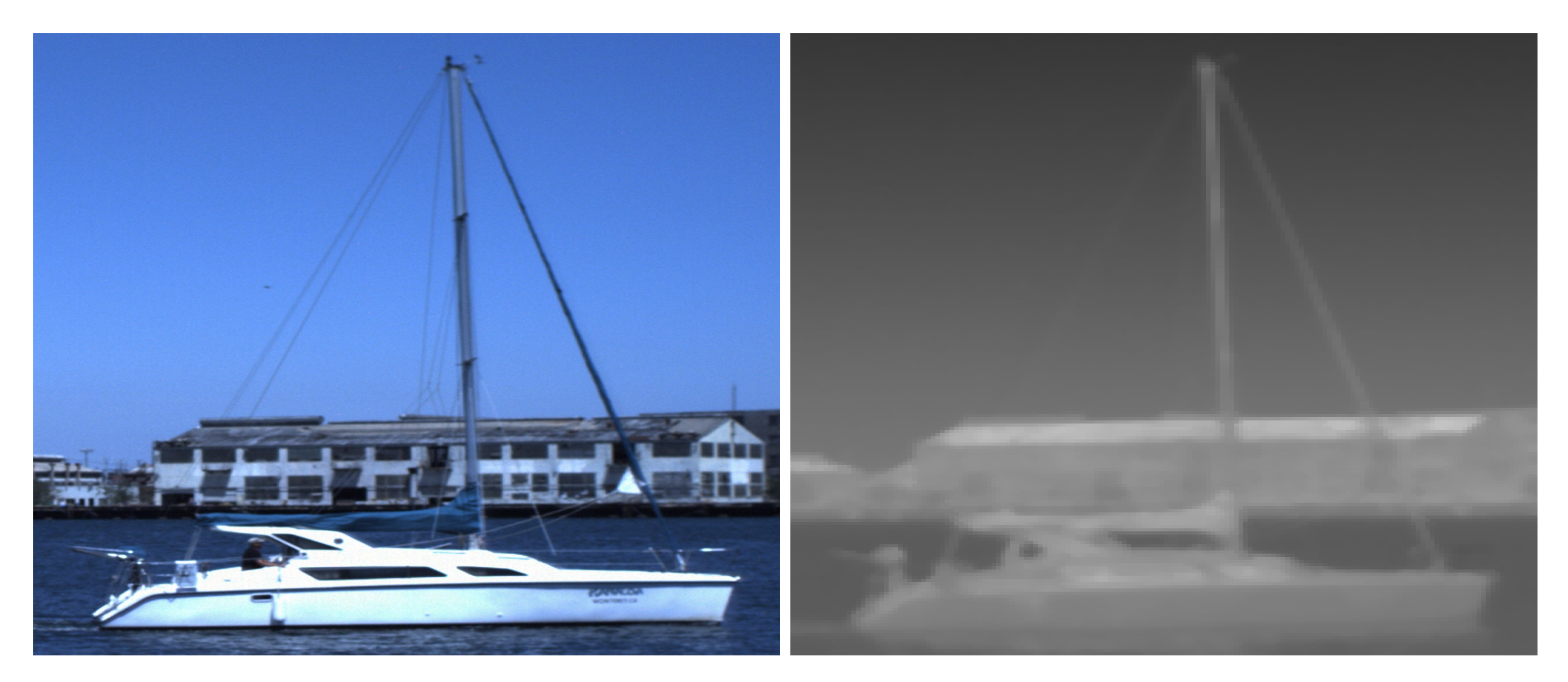
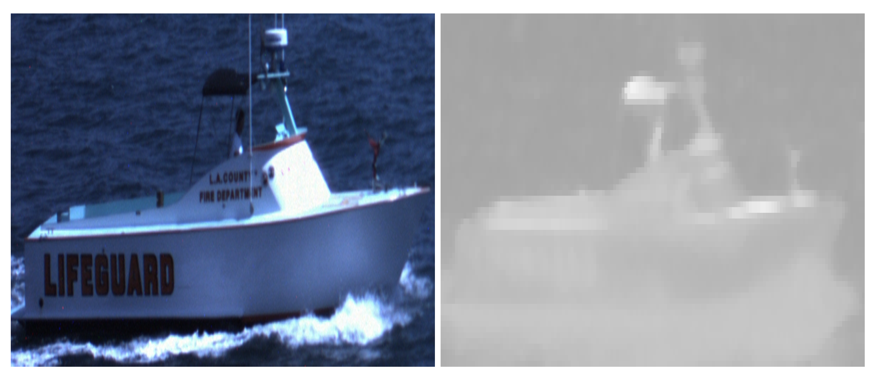
5. Results

Aiming at the problem of multi-sensor target recognition, this paper proposes a new method based on the complementary characteristics of sensors in the fusion of neutrosophic set, which improves the accuracy of target type recognition. Using the identification of the sea surface vessel type as the verification scenario, the category-oriented sensor complementarity vector is constructed through feature extraction, sensor training of the target’s infrared and visible image training data. The multi-sensor neutrosophic set model is performed on the target to be recognized to realize the multi-sensor. Compared with other methods, the method proposed in this paper performs better in recognition accuracy, Compared with other fuzzy mathematics theories, the neutrosophic set theory is more helpful for us to deal with the complementary information between sensors. At the same time, the three sets of functions included in the neutrosophic set allow us to flexibly adjust the weight and other parameters, and the calculation of the neutrosophic set is simple, it takes less time to run the program. Further research will mostly concentrate on the the proposed method can be used to more complicated study to further demonstrate its efficiency.